Commensurability oscillations in a quasi-two-dimensional electron gas
subjected to strong in-plane magnetic field

Abstract

We report on a theoretical study of the commensurability oscillations in a quasi-two-dimensional electron gas modulated by a unidirectional periodic potential and subjected to tilted magnetic fields with a strong in-plane component. As a result of coupling of the in-plane field component and the confining potential in the finite-width quantum well, the originally circular cyclotron orbits become anisotropic and tilted out of the sample plane. A quasi-classical approach to the theory, that relates the magneto-resistance oscillations to the guiding-center drift, is extended to this case.

I Introduction

An isotropic quasi-two-dimensional electron system with circular Fermi contours undergoes the Lifshitz phase transition Lifshitz under the influence of a strong in-plane magnetic field. The topology of Fermi contours changes. The deviation from the circular shape depends on the magnetic field strength and the form of the confining potential. In systems with two occupied subbands the excited subband is emptied at a certain critical in-plane field, and the corresponding second Fermi loop disappears.

The Fermi contours acquire an asymmetric egg-like shape in an asymmetric triangular potential at the hetero-interface.Heisz1993 ; Smrcka.JP.1993 In wide quantum wells and double wells with a single occupied subband the Fermi contours resemble the Cassini oval: as the in-plane magnetic field increases the elongated convex curves acquire the concave peanut-like shape. At high in-plane fields the single Fermi line is split into two parts.Lyo.PRB.95 ; Smrcka.JP.1995

The deformation of a Fermi contour shape can be characterized by a single experimentally measurable quantity, the magnetic-field-dependent cyclotron mass.Smrcka.JP.1993 ; Smrcka.JP.1995 Its field-dependence can be studied e.g. by the cyclotron resonance in the infrared region of the optical spectra Kuriyama.SSC.1999 ; Takaoka.PhysB.2001 ; Takaoka.PhysE.2001 ; Aikawa.PhysE.2002 ; Marlow.PhysB.98 or the temperature damping of Shubnikov-de Haas oscillations. Smrcka.PRB.95 ; Schneider.PhysB.01 ; Hatke.PRB.12 The closely related magnetic-field dependence of the density of states is reflected in a resistance oscillation measured as a function of the in-plane magnetic field. Jungwirth.PRB.1997 ; Makar.PRB.00

More details about the size and shape of cyclotron orbits can be gained from the magneto-electron focusing experiments and the commensurability oscillations measurement. Ohtsuka.PB.1998 ; Oto.PE.2001

The commensurability oscillations Weiss.EP.1989 ; Winkler.PRL.1989 ; Gerhardts.PRL.1989 ; Beenakker.PRL.1989 – oscillations of the magnetoresistance, measured at low temperatures and in a low perpendicular magnetic field in the presence of a weak modulation potential – are periodic in the inverse field. Their period reflects the commensurability of the cyclotron orbit diameter and the modulation period.

The first usage of the commensurability oscillations measurement in strong in-plane magnetic fields was to confirm the distortion of the Fermi contour to the egg-like shape.Oto.PE.2001 Two experimental arrangements were examined — with a lattice vector of the unidirectional lateral superlatices either parallel or perpendicular to the in-plane magnetic-field component. The observed results were consistent with the theoretical prediction.

The influence of the Fermi loop egg-like deformation on the chaotic electron dynamics in a two-dimensional antidot lattice was studied both theoretically and experimentally. Reasonable agreement between the theory and the experiment was achieved.Soto.Micro.00 ; Soto.PRB.02

Recently, the commensurability oscillations were investigated in detail in a wide double hetero-junction well with an occupied bonding subband and a unidirectional modulation potential.Kamburov.PRB.2013 The caliper dimensions of the in-plane field distorted Fermi contours obtained from the experimental data were compared with the results of the first-principle self-consistent calculation. An overall semi-quantitative agreement was achieved between the experimental and the theoretical results. However, a systematic discrepancy was found between the observed and the calculated elongation of the Fermi contour for the case of a lattice vector parallel to the in-plane magnetic field.

To shed light on this apparent discrepancy between the theoretical and the experimental findings, we try to extend the quasi-classical approach, that relates the magnetoresistance oscillations to the guiding-center drift, to the case of cyclotron orbits which are anisotropic and tilted out of the sample plane.

II Cyclotron orbits in tilted magnetic field

Let us consider a single bonding subband of a symmetric wide well or a double well.Smrcka.JP.1993 ; Smrcka.JP.1995 Assuming the in-plane magnetic field parallel to $y$-axis, the Fermi contour in the $k_{x}-k_{y}$ plane is described by an expression

$$E_{F}=E(k_{x})+\frac{\hbar^{2}k_{y}^{2}}{2m},$$ (1)

where $E_{F}$ denotes the Fermi energy. Only the $k_{x}$-dependence of the energy is influenced by the in-plane field, $B_{y}$, while the harmonic dependence of the energy on the wave vector component $k_{y}$ remains untouched. With increasing $B_{y}$ the curvature of $E(k_{x})$ decreases for $k_{x}$ close to $k_{x}=0$ and, at a certain value of $B_{y}$, becomes negative. A local maximum develops at $k_{x}=0$, accompanied by two new minima positioned symmetrically around it. The corresponding Fermi contours resemble the Cassini ovals: the convex curves elongated in $k_{x}$-direction acquire the concave peanut-like shape at higher fields with the width of a peanut ‘waist’ at $k_{x}=0$ shrinking to zero as $B_{y}$ increases.

The quasi-classical theory predicts that in a weak perpendicular magnetic field $B_{z}$ an electron is driven around a Fermi contour by the Lorentz force with the velocity components given by $v_{x}=1/\hbar\,\partial E(k_{x})/\partial k_{x}$ and $v_{y}=\hbar k_{y}/m$. The related real-space cyclotron orbits are similar in shape, but scaled by $\ell_{z}^{2}=\hbar/(|e|B_{z})$ and rotated by $\pi/2$, as $v_{x}=\ell_{z}^{2}\,dk_{y}/\!dt$ and $v_{y}=-\ell_{z}^{2}\,dk_{x}/\!dt$.

From these expressions we can calculate the in-plane field-dependent period of the cyclotron motion $T$, or equivalently the cyclotron frequency $\omega_{c}=|e|B_{z}/m_{c}$, where the cyclotron effective mass $m_{c}$ is related to the shape of the Fermi contour by

$$m_{c}=\frac{\hbar^{2}}{2\pi}\oint\frac{dk}{|\nabla_{k}E|}=\frac{\hbar}{2\pi}\oint\frac{dk}{\sqrt{v_{x}^{2}+v_{y}^{2}}}.$$ (2)

From here we obtain the density of states $g$:

$$g=\frac{m_{c}}{\pi\hbar^{2}}.$$ (3)

Eq.(2) also determines the relation between the electron concentration $N$ and the Fermi energy $E_{F}$ through $N=gE_{F}$. In zero in-plane field this relation reduces to $E_{F}=\hbar^{2}k_{F}^{2}/2m$, where the Fermi wave vector $k_{F}$ is given by $k_{F}=\sqrt{2\pi N}$.

Thus, assuming that the coordinates of a guiding center in $x-y$ plane are $X$ and $Y$, the time dependence of an electron motion along the real-space orbits is described by equations

$$x(t)=X+\ell_{z}^{2}k_{y}(t),\,\,\,y(t)=Y-\ell_{z}^{2}k_{x}(t).$$ (4)

Due to the finite well width $d$ the real-space orbit has also a $z$-coordinate:Smrcka.JP.1995

$$z(t)=\ell_{y}^{2}\left(k_{x}-\frac{\hbar v_{x}}{m}\right),$$ (5)

where $\ell_{y}^{2}=\hbar/(|e|B_{y})$.

Two new important features appear when compared with previously discussed zero-in-plane-field cyclotron orbits.

First, the velocity of an electron moving along an orbit is no longer constant and depends on its position on the Fermi contour. Most pronounced changes go for the so called turning points, i.e., the points on the Fermi contour where one of the velocity components drops to zero. While in the zero-field case there were only two pairs of turning points at crossings of the Fermi contour with the $k_{x}$ and $k_{y}$ axes, new turning points appear when the Fermi contour becomes concave. Their position on a Fermi line is related to field-induced new minima of $E(k_{x})$.

Second, as follows from Eqs.(4,5) the cyclotron orbit is tilted. The $z$-coordinate of an electron does not remain in the center of a well, and the electron moves from one side of a well to the other when traveling along a real space path.

III Commensurability oscillations

The quasi-classical description of the commensurability oscillations – the magneto-resistance oscillations due to the presence of a weak unidirectional potential – is based on the solution of the Boltzmann equation in the relaxation time approximationBeenakker.PRL.1989 . The oscillations are periodic in $1/B_{z}$ and their amplitude is proportional to the mean square drift velocity averaged over the positions of the guiding centers. The drift velocity of a given guiding center can be calculated by the time-average of an oscillating electric field seen by an electron traveling around the center along the real-space cyclotron orbit.

In zero in-plane magnetic field the cyclotron orbits are circles with a radius $R=\ell_{z}^{2}\,k_{F}$. If we assume a sinusoidal potential with the lattice vector ${\bf a}$ oriented along the $y$-axis, the decisive contributions to the drift velocity are obtained at the two turning points $Y+R$ and $Y-R$, where an electron stops for a while, before the velocity component $v_{y}$ changes sign.

It was shownWeiss.EP.1989 that the frequency $f$ of commensurability oscillations is proportional to the radius of the Fermi contour $k_{F}$ by

$$f=\frac{2\hbar}{|e|a}k_{F},$$ (6)

i.e., the frequency $f$ measures the caliper dimension of the Fermi contour.

In the following we discuss why the above formula cannot be simply extended to the case of non-circular Fermi contours by replacing $k_{F}$ by the Fermi contour calipers, which determine the position of the turning points on the real space orbits.

In finite $B_{y}$, the time-averaged electric field of the orbit with the guiding center coordinate $Y$ is given by

$$\mathcal{E}(Y)=\int_{0}^{T}\mathcal{E}_{0}\bigl{(}z(t)\bigr{)}cos\left(\frac{2\pi}{a}y(t)\right)dt.$$ (7)

The corresponding drift velocity reads $v_{\textrm{drift}}=\mathcal{E}(Y)/B_{z}$, the dependence of $y$ and $z$ coordinates on time is described through the time dependent $k_{x}$ by Eqs.(4,5).

When compared with the zero-field case, the main difference stems from the following facts.

There are four more turning points for concave Fermi contours where the velocity components drop to zero, as shown in the Fig.(1).

Moreover, we assume that the source of the unidirectional periodic modulation is only on one side of a quantum well and therefore the modulation potential is partly screened by the quasi-two-dimensional electron layer of a finite width. Then the strength of the oscillating electric field is $z$-dependent and need not be the same on both sides of a well.

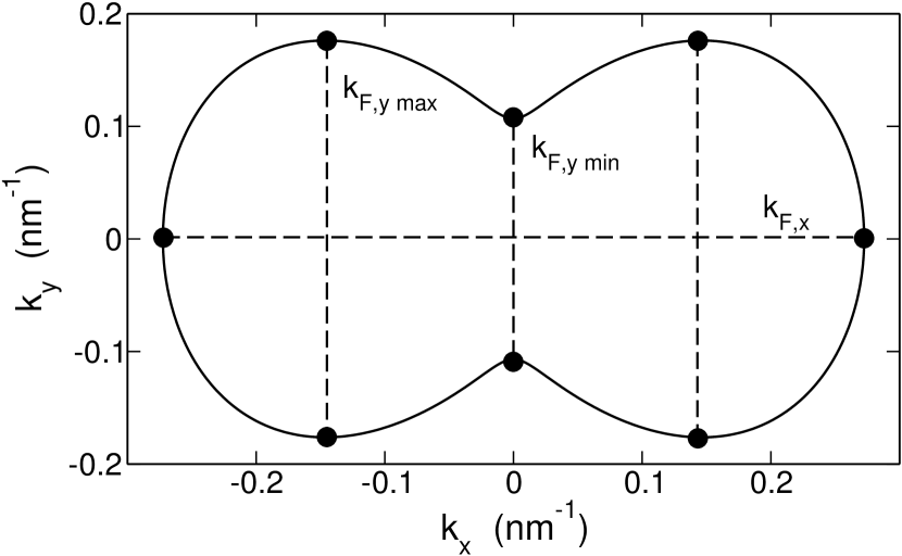
Figure 1: The caliper dimensions of the concave Fermi contour at $B_{y}=8\,\textrm{T}$. Dots mark the turning points on the related cyclotron orbits rotated by $\pi/2$ and multiplied by $\ell_{z}^{2}$.

As mentioned above, the transport coefficients obtained by the solution of the Boltzmann equation, or from the linear response theory,Gerhardts.PRL.1989 ; Winkler.PRL.1989 depend on the mean square of the drift velocities. It was shown by both methods that ${\Delta\varrho_{yy}}$, the change of the magneto-resistance in the presence of a weak unidirectional potential, is proportional to the mean square drift velocity averaged over $Y$,

$$\frac{\Delta\varrho_{yy}}{\varrho_{0}}\,\propto\,\frac{\omega_{z}^{2}\tau^{2}}{\sigma_{0}}\frac{1}{a}\int_{0}^{a}v_{\textrm{drift}}^{2}(Y)dY=\frac{\omega_{z}^{2}\tau^{2}}{\sigma_{0}}\langle v_{\textrm{drift}}^{2}\rangle.$$ (8)

Here $\tau$ is the relaxation time, $\varrho_{0}$ and $\sigma_{0}$ are the resistivity and conductivity at $B_{z}=0$, respectively.

Similar expressions can be written for the lattice vector oriented along the $x$-direction.

IV Model calculation

To illustrate the relevance of the above extension of the quasi-classical description of commensurability oscillations we present the results of a numerical calculation based on the simple tight-binding model of a double well.Hu.PRB.92 ; Lyo.PRB.94 ; Kurobe.PRB.94 This model captures quite well the essence of physics of double wells and wide quantum wells subjected to a strong in-plane magnetic field.

We consider two strictly two-dimensional electron layers in very narrow quantum wells separated by a barrier. The model is characterized by two parameters, the interlayer distance $d$ and the hopping integral $t_{h}$. Such a system represents the first step from strictly two-dimensional to three-dimensional structures.

The diagonalization of a $2\!\times\!2$ matrix yields the $k_{x}$-dependence of the bonding subband energy in the form

$$E(k_{x})=\frac{\hbar^{2}k_{x}^{2}}{2m}+\frac{e^{2}d^{2}B_{y}^{2}}{8m}-\sqrt{\delta^{2}+t_{h}^{2}},$$ (9)

where $\delta$ is the abbreviation for $\hbar|e|dB_{y}k_{x}/2m$. The Fermi energy $E_{F}$ corresponding to the fixed concentration of carriers $N$ is determined by Eqs. (2,3). Here we choose $N=8\times 10^{11}\,\textrm{cm}^{-2}$, $d=20\,\textrm{nm}$ and $t_{h}=2\,\textrm{meV}$. A few examples of cyclotron orbits calculated based on these parameter are presented in the Fig.2.

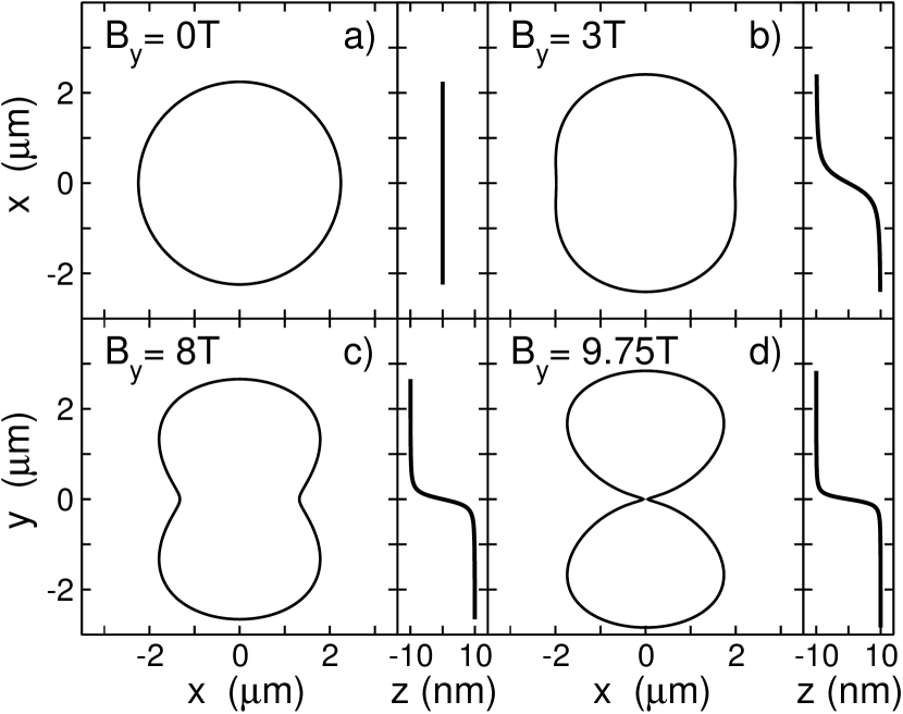
Figure 2: Projections of cyclotron orbits on the $x-y$ and $y-z$ planes, $B_{z}\approx 0.07\,\textrm{T}$. a) $B_{y}=0\,\textrm{T}$. The orbit is circular and lies in the middle of a double well at $z=0$. b) $B_{y}=3\,\textrm{T}$. The orbit is on the border between the convex and concave curve. The $z$-coordinate changes sign at $y=0$. c) $B_{y}=8\,\textrm{T}$. The concave shape of the orbit is fully developed. An electron spends most time near the opposite sides of the structure at $z=\pm d/2$. d) $B_{y}=9.75\,\textrm{T}$. The orbit is close to splitting. The change of sign of the $z$-coordinate near $y=0$ is very sharp.

The $B_{z}$-dependence of commensurability oscillations is given by Eqs.(7) and (8). These expressions were evaluated by numerical integration for the fixed in-plane field components $B_{y}$ between $0$ and $9.75\,\textrm{T}$. The domain of $B_{z}$ was chosen between $0.05$ and $0.35\,\textrm{T}$. This is consistent with a range of fields commonly used in experiments – below the minimum field the oscillations are usually damped, above the maximum field the Shubnikov-de Hass oscillations dominate. Note that this choice is not an inherent property of the quasi-classical approach. But, as it will be shown later, it can slightly influence interpretation of our model calculation.

To test the accuracy of our numerical method, besides of $\langle v_{\textrm{drift}}^{2}\rangle$ we also calculate the averaged drift velocity $\langle v_{\textrm{drift}}\rangle$. It defines the macroscopic current $e\langle v_{\textrm{drift}}\rangle$ through the sample which must, of course, disappear in the thermodynamic equilibrium.

We first test our model on two examples: the standard circular Fermi contour at $B_{y}=0\,\textrm{T}$ and a strongly anisotropic Fermi contour at $B_{y}=8\,\textrm{T}$. The output of our model calculation is presented in the Fig.3.

The results for a circular Fermi contour are shown in the Fig.3​ a). They agree with results published previously, the oscillations reach zero in each period and their frequency satisfies the commensurability condition $f=\frac{2\hbar}{|e|a}\,k_{F}$, given by Eq.(6). The period of oscillations is the same for a lattice vector ${\bf a}$ oriented along the $x$ and $y$-axes. The reason is that an electron traveling along the circular orbit stays all the time in the middle of the structure, $z=0$, and, therefore, the $z$-dependence of a modulation potential plays no role.

The case of anisotropic Fermi contours is quite different. The dependence of oscillations on the lattice vector orientation is strong and the $z$-dependence of the modulation potential can play an important role.

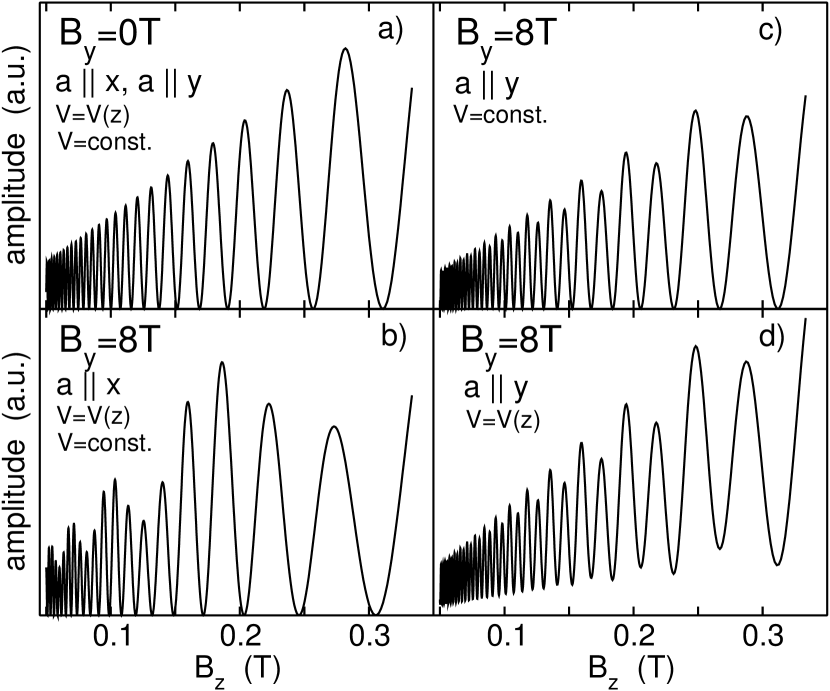
Figure 3: Commensurability oscillations as a function of $B_{z}$. a) $B_{y}=0\,\textrm{T}$. The orbit is circular and the same form of oscillations for ${\bf a}\!\parallel\!x$ and ${\bf a\!}\parallel\!y$ is obtained. The $z$-dependence of a modulation potential plays no role. b) $B_{y}=8\,\textrm{T}$, ${\bf a}\!\parallel\!x$. Again, the $z$-dependence of a modulation potential plays no role, as an electron feels the same electric field at $x$ and $-x$. c) $B_{y}=8\,\textrm{T}$, ${\bf a}\!\parallel\!y$ and a $z$-independent modulation potential. Two frequencies of oscillations are resolved, their aplitude reaches zero. d) $B_{y}=8\,\textrm{T}$, ${\bf a}\!\parallel\!y$ and a $z$-dependent modulation potential. An electron feels different electric fields at $y$ and $-y$. The amplitude of oscillations does not drop to zero. The weights of two frequencies in the frequency spectrum are changed.

Let us first consider the lattice vector ${\bf a}$ parallel to the $x$-axis. As in the previous case, $B_{y}=0\,\textrm{T}$, the $z$-dependence of the modulation potential has almost no influence on the resulting shape of commensurability oscillations, shown in the Fig.3​ b). The reason is that the $z$-coordinate depends only on $k_{x}$ and an electron feels the same electric field at $x$ and $-x$. The fast Fourier transform (FFT) of oscillations yields three frequencies related to four turning points which correspond to $\pm\,k_{F,y\textrm{ max}}$, two turning points corresponding to $\pm\,k_{F,y\textrm{ min}}$, and their average.

Now we turn our attention to ${\bf a}\!\parallel\!y$ and a $z$-independent modulation potential. The calculated results are presented in the Fig.3 c). The FFT of oscillations yields two frequencies close to $f_{1}=\frac{2\hbar}{|e|a}\,k_{F,x}$ and $f_{2}=\frac{\hbar}{|e|a}\,k_{F,x}$. As mentioned above their deviations from the exact values and their weights in the frequency spectrum depend slightly on the chosen domain of $B_{z}$. The frequency $f_{1}$ is related to the turning points $\pm\,k_{F,x}$ shown in Fig.1. The frequency $f_{2}$ appears for the first time at the critical field $B_{y}$ for which the Fermi contour becomes concave, in our case at $B_{y}=3\,\textrm{T}$. The weight of $f_{2}$ in the frequency spectrum increases with increasing $B_{y}$ and reaches maximum at a critical field $B_{y}=9.75\,\textrm{T}$ above which the Fermi contour splits. The reason is that at this field both velocity components $v_{x}$ and $v_{y}$ drop to zero at ${\bf k}=0$. Note that the period of cyclotron motion $T$ and the cyclotron mass $m_{c}$, given by Eq.(2), also have a singularity for the same reason here.

Next we consider ${\bf a}\!\parallel\!y$ and a $z$-dependent modulation potential. The $z$-dependence of the modulation affects mainly the role of a real-space trajectory in the vicinity of the turning points related to $k_{F,x}$ and $-k_{F,x}$. According to Eq.(5) the $z$-coordinate depends on $k_{x}$ and an electron sees different electric fields near these two points. As a consequence, the electric field averaged over the cyclotron orbit is modified. The amplitude of oscillations does not drop to zero, as can be seen in the Fig.3 d), and the weights of frequencies $f_{1}$ and $f_{2}$ in the frequency spectrum change.

The main results of our model calculations are shown in the Fig.4. The evolution of the Fermi contour calipers in the in-plane magnetic field $B_{y}$ is presented together with the values derived from the FFT of commensurability oscillations. The oscillations were calculated assuming a $z$-dependent modulation potential that yielded the reduced electric field in the second layer. Here $\mathcal{E}(-d/2)=0.4\times\mathcal{E}(d/2)$ was chosen.

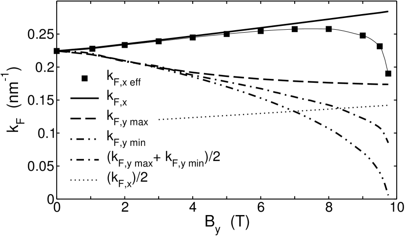
Figure 4: The in-plane field dependence of the Fermi contour caliper dimensions. For ${\bf a}\parallel x$ the $k_{F,y\textrm{ max}}$ splits into $k_{F,y\textrm{ min}}$ and $(k_{F,y\textrm{ max}}+k_{F,y\textrm{ min}})/2$ above the critical field $B_{y}$ for which the Fermi contour becomes concave. For ${\bf a}\parallel y$, the value $k_{F,x\textrm{ max}}/2$ appears abruptly at this critical field. An effective $k_{F,x\textrm{ eff}}$ is derived from the weighted average of frequencies $f_{1}$ and $f_{2}$ corresponding to those vectors.

Our calculation does not take into account the line broadening by the inaccuracy of instruments, by the finite temperature and/or by electron scattering. On the other hand, the line broadening strongly influences interpretation of experimental data. Even in the most recent measurements Kamburov.PRB.2013 only one frequency was resolved in oscillation spectra measured both for ${\bf a}\parallel x$ and ${\bf a}\parallel y$. For the case of ${\bf a}\parallel x$ the good agreement with the frequency corresponding to $k_{F,y\textrm{ max}}$ was found, for ${\bf a}\parallel y$ the measured frequency is between $f_{1}$ and $f_{2}$ mentioned above.

In our calculation, which does not take into account the line broadening, the agreement between the Fermi contour calipers and the values derived from the FFT is very good for ${\bf a}\parallel x$. Therefore only the curves corresponding to contour calipers are plotted in the Fig.4 as functions of $B_{y}$. The $k_{F,y\textrm{ max}}$ splits into $k_{F,y\textrm{ min}}$ and $(k_{F,y\textrm{ max}}+k_{F,y\textrm{ min}})/2$ above the critical field $B_{y}$ for which the Fermi contour becomes concave. The weight of the frequency related to $k_{F,y\textrm{ max}}$ dominates.

The case of ${\bf a}\parallel y$ is different. For $B_{y}$ below the critical value only the peak related to $f_{1}$ is observed in the FFT spectrum. The second peak corresponding to $f_{2}=f_{1}/2$ appears with a very small weight at the critical field and dominates at high fields. To mimic the experimental results, which resolve only one frequency, we plot an effective $k_{F,x\textrm{ eff}}$, derived from the weighted average of frequencies $f_{1}$ and $f_{2}$, except of the values based on the frequencies $f_{1}$ and $f_{2}$ themselves.

V Summary and conclusions

We have studied the commensurability oscillations in a quasi-two-dimensional electron gas modulated by a unidirectional periodic potential and subject to tilted magnetic fields with a strong in-plane component. A quasi-classical approach to the theory, that relates the magneto-resistance oscillations to the guiding-center drift was employed. A systematic discrepancy between the observed and the calculated elongation of the Fermi contour for the in-plane magnetic field parallel to the lattice vector, found in  Kamburov.PRB.2013 , is explained by the in-plane magnetic-field distortion of the cyclotron orbits .

Our arguments are as follows: First, the velocity of an electron moving along an orbit is no longer constant and depends on its position on the Fermi contour. Second, the cyclotron orbit is tilted, the electron moves from one side of a well to the other, and sees the different strengths of the one-side-modulation potential on the different well sides.

The numerical simulation is based on the simple tight-binding model of a double well, the spin of electrons is not taken into account.

VI Acknowledgements

This work was supported by grant Nr. LM2011026 of the Ministry of Education of the Czech Republic. J. Kučera is ackowledged for his careful reading of the manuscript.

References

- (1) I. M. Lifshitz, Sov. Phys. JETP 11, 1130 (1960).
- (2) J.M. Heisz and E. Zaremba, Semicond. Sci. Technol. 8, 575 (1993).
- (3) L. Smrčka and T. Jungwirth, J. Phys.: Condens. Matter 6, 55 (1993).
- (4) S. K. Lyo, Phys. Rev. B 51, 11160 (1995).
- (5) L. Smrčka and T. Jungwirth, J. Phys.: Condens. Matter 7, 3721 (1995).
- (6) A. Kuriyama, S. Takaoka, K. Oto, K. Murase, S. Shimomura, S. Hiyamizu, M. Cukr, T. Jungwirth, and L. Smrčka. Solid State Communications 111, 699 (1999)
- (7) S. Takaoka, H. Aikawa, K. Oto, and K. Murase, Physica B 298 (2001).
- (8) S. Takaoka, H. Aikawa, K. Oto, and K. Murase Physica E 11 194 (2001).
- (9) H. Aikawa, S. Takaoka, K. Oto, K. Murase, T. Saku, Y. Hirayama, S. Shimomura, and S. Hiyamizu Physica E 12 578 (2002).
- (10) T. P. Marlow, D. D. Arnone, C. L. Foden, E. H. Linfield, D. A. Ritchie, and M. Pepper, Physica B 249, 966 (1998).
- (11) L. Smrčka, P. Vašek, J. Koláček, T. Jungwirth, and M. Cukr, Phys. Rev. B 51, 18011 (1995).
- (12) D. Schneider, T. Klaffsa, K. Pierzb, and F.-J. Ahlers, Physica B 298, 234 (2001).
- (13) A. T. Hatke, M. A. Zudov, L. N. Pfeiffer, and K. W. West, Phys. Rev. B 89, 241305 2012.
- (14) T. Jungwirth, T. S. Lay, L. Smrcka, and M. Shayegan, Phys. Rev. B 56, 1029 (1997).
- (15) O. N. Makarovskii, L. Smrčka, P. Vašek, T. Jungwirth, M. Cukr, and L. Jansen, Phys. Rev. B 62 10908 (2000).
- (16) K. Ohtsuka, S. Takaoka, K. Oto, K. Murase, and K. Gamo, Physica B 249, 780 (1998).
- (17) K. Oto, S. Takaoka, K. Murase, and K. Gamo, Physica E 11, 177 (2001).
- (18) D. Weiss, K. von Klitzing, K. Ploog, and G. Weimann, Europhys. Lett. 8, 179 (1989).
- (19) R. W. Winkler, J.P. Kotthaus, and K. Ploog, Phys. Rev. Lett. 62, 1177 (1989).
- (20) R. R. Gerhardts, D. Weiss, and K. von Klitzing, Phys. Rev. Lett. 62, 1173 (1989).
- (21) C. W. J. Beenakker, Phys. Rev. Lett. 62, 2020 (1989).
- (22) N. M. Sotomayor, G. M. Gusev, J. R. Leite, and V. A. Chitta, Microelectronic Engineering 51 111 (2000).
- (23) N. M. Sotomayor, G. M. Gusev, J. R. Leite A. A. Bykov, L. V. Litvin, D. K. Maude, and J. C. Portal, Phys. Rev. B 66 035324 (2002).
- (24) D. Kamburov, M. A. Mued, M. Shayegan, L. N. Pfeiffer, K. W. West, K. W. Baldwin, J. J. D. Lee, and R. Winkler, Phys. Rev. B 88, 125435 (2013).
- (25) J. Hu and A. H. MacDonald, Phys. Rev. B 46, 12 554 (1992).
- (26) S. K. Lyo, Phys. Rev. B 50, 4965 (1994).
- (27) A. Kurobe, I. M. Gastleton, E. H. Linfield, M. P. Grimshaw, K. M. Brown, D. A. Ritchie, M. Pepper, and G. A. C. Jones, Phys. Rev. B 50, 4889 (1994).