Photoassociation of Universal Efimov Trimers

Abstract

In view of recent experiments in ultracold atomic systems, the photoassociation of Efimov trimers, composed of three identical bosons, is studied utilizing the multipole expansion. We study both the normal hierarchy case, where one-body current is dominant, and the strong hierarchy case, relevant for photoassociation in ultracold atoms, where two-body current is dominant. For identical particles in the normal hierarchy case, the leading contribution comes from the $r^{2}$ $s$-mode operator and from the quadrupole $d$-mode operator. The $s$-mode reaction is found to be dominant at low temperature, while as the temperature increases the $d$-mode becomes as significant. For the strong hierarchy case, the leading contribution comes from a 2-body $s$-wave $\delta$ operator. In both cases log periodic oscillations are found in the cross section. For large but finite scattering length the amplitude of the oscillations becomes larger in comparison to infinite scattering length case. We apply our theory to photoassociation of ⁷Li ultracold atoms and show a good fit to the available experimental results.

1 Introduction

When the properties of a few-body or many-body system are insensitive to the details of the microscopic interaction between its constituents, the system is said to be Universal. A free gas is the simplest and somewhat trivial example of universality. A very rich and important case is a system governed by the low energy scattering parameters. Such scenario can be realized in ultra cold atomic systems, where the two-body scattering length can be tuned by a Feshbach resonance to be much larger than any other length scale in the system [1, 2].

The trimer, or the three body system, attracts special attention as the simplest non-trivial universal system. Moreover, in the 70’s Efimov predicted that in the limit of a resonant 2-body interaction, the system reveals universal properties [3, 4]. A peculiar prediction is the existence of a series of giant three body molecules, known as Efimov trimers, that was verified experimentally a few years ago. For a review see Ref. [5] and references therein.

The coupling of a radiation field with the system is a useful experimental tool in physics. The photoassociation and photodissociation processes are sensitive ways to measure spectrum and also other properties of few and many-body systems [6]. Recently, trimers were formed by radio-frequency (rf) excitations in both fermionic ⁶Li [7, 8] and bosonic ⁷Li [9] systems.

In a previous work [10], we have presented the multipole analysis of an rf association process binding a molecule of $N$ identical bosons. We have considered two different scenarios relevant to photoassociation experiments in neutral ultra cold atoms, confined in a strong magnetic field: (i) spin-flip process, and (ii) frozen-spin process.

In the spin-flip mechanism, the photon induces a spin state change in the absorbing atom, and most of its energy is dedicated transferring the atom from one hyperfine state to another. The typical energy of the photon in this case is of the order of the hyperfine splitting. The spin-flip mechanism was materialized experimentally by [7, 8]. Previous analysis of rf experiments [11, 12, 13, 14, 15], which relied on the Franck-Condon factor, is appropriate for describing these spin-flip reactions.

In the second, frozen-spin, mechanism, the photon energy is insufficient to bridge the hyperfine gap and therefore the atom spin is “frozen” throughout the process. In this case the photon induces a molecular bound-free transition and the typical photon energy is of the order of the molecular binding energy.

In [10] we have shown that the spin-flip and frozen-spin processes differ by their operator structure and by the de-excitation modes that contribute to the photoassociation rate. The photoassociation experiments carried out by the Bar-Ilan group, see e.g. [9], relied on the frozen-spin mechanism.

We have studied one-body current in frozen-spin reactions, dealing with dimer formation [10], and also calculated numerically the quadrupole response of a bound bosonic trimer [16]. Recently we have identified another scenario, where two-body currents dominate the frozen-spin process, and explored the occurrence of log-periodic oscillations in the reaction cross section [17].

Here, we study few more aspects of the three body photoassociation process. These are (i) The interplay between the $s$-mode and the $d$-mode reaction channels at different temperatures and photon energies, (ii) The effect of finite scattering length on the reaction rate. We utilize the hyperspherical coordinates with the adiabatic expansion to study the trimer photoassociation process, for both one-body process as well as for the two-body process. Analytic results for the transition rates at the unitary point (where the scattering length diverges) are derived using the zero-range approximation, and numerical calculations complete the picture for a large but finite scattering length. Similarly to the dimer case [10], the $s$-mode and the $d$-mode are found to be the leading order contributions in the one-body process. The relative importance of these modes depends on the temperature, where at low temperature the $s$-mode is dominant while at higher temperature the $d$-mode becomes as significant. For both one-body and two-body processes, log-periodic oscillations modulate the cross section. We found that comparing with the unitary point, the amplitude of these oscillations is somewhat larger for finite scattering lengths.

As a concrete example for the usefulness of our approach we analyze the dimer and trimer photoassociation experiments carried out by the Bar-Ilan group in an ultracold atomic ⁷Li gas [9]. As already pointed out, the photoassociation mechanism in these experiments is the frozen spin process. Due to the strong hierarchy, see Sec. 2, the coupling of the photon to the system is dominated by the 2-body magnetization current. Our theory fits well to the available experimental results.

The paper is organized as follows, in section 2 we introduce our model and reiterate the multipole and the currents expansions, describing the interaction of an rf field with the atomic system. In section 3 we introduce the three-body problem and solve it using the hyperspherical adiabatic expansion. The transition matrix elements are calculated in section 4 for infinite, and also for large but finite, scattering lengths. The transition rates are calculated in section 5, and a detailed comparison to experiment is presented in section 6. Section 7 concludes our study.

2 The model

In photoassociation experiments [7, 8, 9], a few MHz rf radiation field is applied to the ultracold atomic gas. Stimulated emission occurs when the photon energy matches the difference between the ultracold gas atoms and the molecule energy, resulting in molecule formation. The transition rate of such process is given by Fermi’s golden rule,

$$r_{i\rightarrow f}=\frac{2\pi}{\hbar}\bar{\sum_{i}}\sum_{f}|\langle f,\mathbf{k}\zeta|\hat{H}_{I}|i\rangle|^{2}\delta(E_{i}-E_{f}-\hbar\omega),$$ (1)

where $\bar{\sum_{i}}$ is an average on the appropriate initial continuum states and $\sum_{f}$ is a sum on the final bound states. The coupling between the neutral atoms and the radiation field takes the form

$$\hat{H}_{I}=-\int d\mathbf{x}\mathbf{\mu}(\mathbf{x})\cdot\nabla\times\mathbf{A}(\mathbf{x})$$

where $\mathbf{\mu}$ is the magnetization density and $\mathbf{A}$ is the electromagnetic field at position $\mathbf{x}$. We have shown [17], that in effective low energy theory [18] $\mathbf{\mu}$ has contributions from one-body current as well as more body currents

$$\mathbf{\mu}(\mathbf{x})=\mathbf{\mu}^{(1)}(\mathbf{x})+\mathbf{\mu}^{(2)}(\mathbf{x})+\ldots.$$ (2)

An effective theory has some UV cutoff $\Lambda$, reflecting some short-range physics which is ignored. Naive power-counting suggests that each order in this expansion is suppressed by a factor of $(Q/\Lambda)^{3}$, where $Q$ is the typical momentum of a particle in the system under consideration. The leading order (LO) one-body current is [19]

$$\mathbf{\mu}^{(1)}(\mathbf{x})=\sum_{j}\mathbf{s}_{j}\mu_{1}\delta(\mathbf{x}-\mathbf{r}_{j}),$$ (3)

where $\mu_{1}$ is the magnetic moment of a single particle, $\mathbf{r}_{j}$ and $\mathbf{s}_{j}$ are the position and the spin of particle $j$. The two-body contribution to the atomic electro-magnetic current enters at the next order (N²LO), or $(Q/\Lambda)^{3}$, and takes the form [19]

$$\mathbf{\mu}^{(2)}(\mathbf{x})=\sum_{i<j}(\mathbf{s}_{i}+\mathbf{s}_{j})\frac{L_{2}}{\Lambda^{3}}\delta(\mathbf{x}-\frac{\mathbf{r}_{i}+\mathbf{r}_{j}}{2})\delta_{\Lambda}(\mathbf{r}_{i}-\mathbf{r}_{j})\;$$ (4)

where $L_{2}=L_{2}(\Lambda)$ is the coupling constant between the radiation field and the four boson fields. The notation $\delta_{\Lambda}(\mathbf{r})$ stands for Dirac’s $\delta$-function smeared over distance $\hbar/\Lambda$.

In the low energy limit $Q\ll\Lambda$, more particles current can be ignored due to suppression by additional $(Q/\Lambda)^{3}$ factor associated with each extra particle field.

Using box normalization of volume $\Omega$, the electro-magnetic field reads

$$\mathbf{A}(\mathbf{x})=\sum_{\mathbf{k},\zeta}\sqrt{\frac{\hbar}{2\Omega\omega\epsilon_{0}}}\hat{e}_{\mathbf{k}\zeta}(a^{\dagger}_{\mathbf{k}\zeta}e^{i\mathbf{k}\cdot\mathbf{x}}+h.c.)$$

where $\zeta=1,2$ are the linear photon polarizations, $\omega$ is the photon frequency, $\mathbf{k}$ its momentum, and $\epsilon_{0}$ is the vacuum permeability.

For bosonic systems confined in a strong (static) magnetic field, the initial and final state atomic wave functions can be written as a product of spin and configuration space terms, $\Psi=\psi_{LM}\chi_{M_{F}}$. The spin wave function $\chi_{M_{F}}$ is the symmetrized function $\chi_{M_{F}}={\cal S}\left[|m_{F}(1)\rangle|m_{F}(2)\rangle\ldots|m_{F}(N)\rangle\right]$ with magnetic quantum number $M_{F}=\sum_{j}m_{F}(j)$. The spatial wave function $\psi_{LM}=\psi_{LM}(\mathbf{r}_{1},\mathbf{r}_{2},\ldots\mathbf{r}_{N})$ is a symmetric function with angular momentum quantum numbers $LM$. Using this factorization, the one-body transition matrix element in (1) takes the form

$$\eqalign{\langle f,\mathbf{k}\zeta|\hat{H}_{I}^{(1b)}|i\rangle=-i\mu_{1}\sqrt{\frac{\hbar}{2\Omega\omega\epsilon_{0}}}\times\\ \sum_{j=1}^{N}\langle\chi^{f}_{M^{\prime}_{F}}|\mathbf{s}_{j}\cdot(\mathbf{k}\times\hat{e}_{\mathbf{k}\zeta})|\chi^{i}_{M_{F}}\rangle\langle\psi^{f}_{L^{\prime}M^{\prime}}|e^{i\mathbf{k}\cdot\mathbf{r}_{j}}|\psi^{i}_{LM}\rangle,}$$ (5)

whereas the two-body part reads

$$\eqalign{\langle f,\mathbf{k}\zeta|\hat{H}_{I}^{(2b)}|i\rangle=-i\sqrt{\frac{\hbar}{2\Omega\omega\epsilon_{0}}}\frac{L_{2}}{\Lambda^{3}}\times\\ \sum_{i<j}^{N}\langle\chi^{f}_{M^{\prime}_{F}}|(\mathbf{s}_{i}+\mathbf{s}_{j})\cdot(\mathbf{k}\times\hat{e}_{\mathbf{k}\zeta})|\chi^{i}_{M_{F}}\rangle\times\\ \langle\psi^{f}_{L^{\prime}M^{\prime}}|e^{i\mathbf{k}\cdot(\mathbf{r}_{i}+\mathbf{r}_{j})/2}\delta_{\Lambda}(\mathbf{r}_{i}-\mathbf{r}_{j})|\psi^{i}_{LM}\rangle.}$$ (6)

Using spherical notation, the spin operator reads $\mathbf{s}\cdot(\mathbf{k}\times\hat{e}_{\mathbf{k}\zeta})=\sum_{\lambda}(-)^{\lambda}s_{-\lambda}\cdot(\mathbf{k}\times\hat{e}_{\mathbf{k}\zeta})_{\lambda},$ where $\lambda=0,\pm 1$. The geometrical factor, $\eta=(\hat{k}\times\hat{e}_{\mathbf{k}\zeta})_{\lambda},$ is maximal (minimal) for the frozen spin $\lambda=0$ case (spin flip $\lambda=\pm 1$ case), when the rf magnetic component is parallel to the static magnetic field.

The photon wavelength of rf radiation is much larger than the typical dimension of the system $R$, therefore $kR\ll 1$ and the lowest order in $kR$ dominates the interaction. When the photon can induce a Zeeman state change, i.e. spin-flip, the leading contribution comes at order $k$. Energy is delivered to the system through the spin matrix element and we can approximate $e^{i\mathbf{k}\cdot\mathbf{r}}\simeq 1$, to get

$$\eqalign{|\langle f,\mathbf{k}\zeta|\hat{H}_{I}^{(1b)}|i\rangle|^{2}=\frac{\mu_{1}^{2}\hbar k\eta^{2}}{2\Omega c\epsilon_{0}}\sum_{\lambda=\pm 1}\\ |\langle\chi^{f}_{M^{\prime}_{F}}|\sum_{j=1}^{N}s_{j,\lambda}|\chi^{i}_{M_{F}}\rangle|^{2}|\langle\psi^{f}_{L^{\prime}M^{\prime}}|\psi^{i}_{LM}\rangle|^{2}\delta_{L,L^{\prime}}\delta_{M,M^{\prime}}.}$$ (7)

The last term on the rhs of (7) is just the Franck-Condon factor, that appears in the commonly used theory of photoassociation, such as Eq. (3) in Ref. [11].

When the rf photon cannot induce change in the spin structure of the system, $\lambda=0$, and we call the process a frozen spin reaction. In this case $M_{F}^{\prime}=M_{F}$, $|\chi^{f}_{M_{F}}\rangle=|\chi^{i}_{M_{F}}\rangle$ and the transition matrix element can be written as

$$\eqalign{\langle f,\mathbf{k}\zeta|\hat{H}_{I}^{(1b)}|i\rangle=&-i\mu_{1}\sqrt{\frac{\hbar}{2\Omega\omega\epsilon_{0}}}k\eta\langle s_{0}\rangle\times\\ &\langle\psi^{f}_{L^{\prime}M^{\prime}}|\sum_{j=1}^{N}e^{i\mathbf{k}\cdot\mathbf{r}_{j}}|\psi^{i}_{LM}\rangle\;,}$$ (8)

where $\langle s_{0}\rangle=\frac{1}{N}\sum_{j}\langle\chi^{i}_{M_{F}}|s_{j,0}|\chi^{i}_{M_{F}}\rangle$ is the average single particle magnetic moment, which plays the role of an effective charge.

In the long wavelength limit, the exponent can be expanded to yield

$$\eqalign{\sum_{j=1}^{N}e^{i\mathbf{k}\cdot\mathbf{r}_{j}}&\approx N+i\sum_{j=1}^{N}\mathbf{k}\cdot\mathbf{r}_{j}-\frac{1}{6}\sum_{j=1}^{N}k^{2}r_{j}^{2}\cr&-\frac{4\pi}{15}\sum_{j=1}^{N}k^{2}r_{j}^{2}\sum_{m}Y_{2-m}(\hat{k})Y_{2m}(\hat{r}_{j}),}$$ (9)

where $Y_{lm}$ are the spherical harmonics. Clearly this expansion has transparent physical meaning. The zero order operator is proportional to 1 and stands for elastic interaction. In photon emission reaction this process is forbidden by energy conservation. Next comes at first order the dipole. Dealing with identical particles, this term is proportional to the center of mass and hence cannot affect internal degrees of freedom. Two operators appear at second order: the $r^{2}$ operator, corresponding to $s$-mode reaction, and the quadrupole terms, corresponding to $d$-mode reaction. Summing over the initial and final magnetic numbers $M$ and $M^{\prime}$, the transition matrix element reads [10]

$$\eqalign{\sum_{M,M^{\prime}}|\langle f,\mathbf{k}\zeta|\hat{H}_{I}^{(1b)}|i\rangle|^{2}=\frac{4\pi\hbar k^{5}\mu_{1}^{2}\eta^{2}}{2\Omega c\epsilon_{0}}\left|\left\langle s_{0}\right\rangle\right|^{2}\\ \left(\frac{1}{6^{2}}|\langle\psi^{f}_{L^{\prime}}\|\sum_{j=1}^{N}r_{j}^{2}Y_{0}\|\psi^{i}_{L}\rangle|^{2}+\frac{1}{15^{2}}|\langle\psi^{f}_{L^{\prime}}\|\sum_{j=1}^{N}r_{j}^{2}Y_{2}(\hat{r}_{j})\|\psi^{i}_{L}\rangle|^{2}\right).}$$ (10)

For the two body current, we can again utilize the long wave approximation $e^{i\mathbf{k}\cdot(\mathbf{r}_{i}+\mathbf{r}_{j})/2}\approx 1$ to get

$$\eqalign{|\langle f,\mathbf{k}\zeta|\hat{H}_{I}^{(2b)}|i\rangle|^{2}=\frac{4\hbar k}{2\Omega c\epsilon_{0}}\frac{L_{2}^{2}\eta^{2}}{\Lambda^{6}}\left|\left\langle s_{0}\right\rangle\right|^{2}\times\\ |\langle\psi^{f}_{L^{\prime}M^{\prime}}|\sum_{i<j}^{N}\delta_{\Lambda}(\mathbf{r}_{i}-\mathbf{r}_{j})|\psi^{i}_{LM}\rangle|^{2}.}$$ (11)

To find the most relevant operators for the photoassociation process one should consider both the low energy expansion (2) and the long wavelength expansion (9). Dealing with trimer photoassociation, the photon energy has to be of the order of the trimer binding energy $E_{3}$. Therefore the long wavelength expansion parameter can be written as $kr\approx\sqrt{E_{3}/Mc^{2}}\approx Q/Mc,$ where we used $r\approx\sqrt{\hbar^{2}/ME_{3}}$. Therefore one should compare the long wavelength expansion parameter, $kr\approx Q/Mc$ to the low energy expansion parameter $Q/\Lambda$. If $Q/\Lambda\ll{\Lambda}/Mc$, the two-body currents appearing at order $(Q/\Lambda)^{3}$ are much smaller than the second order $(kr)^{2}\approx(Q/Mc)^{2}$ terms. This normal hierarchy case is the situation in the limit $Q\longrightarrow 0$. In the other extreme, when $\Lambda\ll Mc$, the two-body current is more important than the one-body current, proportional to $(Q/Mc)^{2}$. This case of strong hierarchy is typical for photoassociation experiments in ultracold atoms [7, 8, 9]. There, the separation between the mass scale and the binding energy is much bigger than the ratio between the scattering length and the effective range.

3 The Three Body Problem

The Schroedinger equation governs the dynamics of a quantum 3 particle system

$$\left(T+W\right)\psi=E\psi,$$ (12)

where $T$ is the kinetic energy operator in the center of mass frame and $W$ is the potential. Here we assume a short range 2-body forces, thus $W=\sum_{i<j}V(|\mathbf{r}_{i}-\mathbf{r}_{j}|)$. To solve this problem we use the hyperspherical coordinates and the adiabatic expansion [20, 21]. In the following section we review these methods and extend them for the $L>0$ case.

3.1 The Hyperspherical coordinates

To eliminate the center of mass motion, we define the Jacobi coordinates,

$$\mathbf{x}_{i}=\sqrt{\frac{1}{2}}(\mathbf{r}_{j}-\mathbf{r}_{k}),\quad\mathbf{y}_{i}=\sqrt{\frac{2}{3}}\left(-\mathbf{r}_{i}+\frac{\mathbf{r}_{j}+\mathbf{r}_{k}}{2}\right)$$

where $\{ijk\}$ is a cyclic permutation of $\{123\}$. The relation between two sets of Jacobi coordinates $(\mathbf{x}_{i},\mathbf{y}_{i})$ and $(\mathbf{x}_{j},\mathbf{y}_{j})$ is given by the kinematic rotation,

$$\left(\begin{array}[]{c}\mathbf{x}_{j}\\ \mathbf{y}_{j}\end{array}\right)=\left(\begin{array}[]{cc}-\cos\phi_{ij}&\sin\phi_{ij}\\ -\sin\phi_{ij}&-\cos\phi_{ij}\end{array}\right)\left(\begin{array}[]{c}\mathbf{x}_{i}\\ \mathbf{y}_{i}\end{array}\right).$$ (13)

For the case of 3 identical particles, $\phi_{ij}=\pm\pi/3$, where the sign is fixed by the parity of the permutation $\{ijk\}$. For each set of Jacobi coordinates we can define a set of hyperspherical coordinates $(\rho,\Omega_{i})$, where $\rho^{2}=x_{i}^{2}+y_{i}^{2},$ $\Omega_{i}=(\alpha_{i},\hat{x}_{i},\hat{y}_{i})$, and $\tan\alpha_{i}=x_{i}/y_{i}.$ Two different sets of hyperspherical coordinates are related through

$$2\sin^{2}\alpha_{j}=1-\cos 2\phi_{ij}\cos 2\alpha_{i}-\gamma_{i}\sin 2\phi_{ij}\sin 2\alpha_{i},$$ (14)

where $\gamma_{i}=\hat{x}_{i}\cdot\hat{y}_{i}.$ The hyperradius $\rho$ is invariant under kinematic rotations, particle permutations, and therefore under change of coordinates sets.

In the hyperspherical coordinates the kinetic energy operator reads,

$$T=-\frac{\hbar^{2}}{2m}\left(\frac{\partial^{2}}{\partial\rho^{2}}+\frac{5}{\rho}\frac{\partial}{\partial\rho}-\frac{\hat{K}^{2}}{\rho^{2}}\right).$$ (15)

Here, $\hat{K}^{2}$ is the square of the grand angular momentum operator,

$$\hat{K}^{2}=-\frac{1}{\sin 2\alpha}\frac{\partial^{2}}{\partial\alpha^{2}}\sin 2\alpha+\frac{\hat{l}^{2}_{x}}{\sin^{2}\alpha}+\frac{\hat{l}^{2}_{y}}{\cos^{2}\alpha}-4\;,$$ (16)

and $\hat{l}_{x}$, $\hat{l}_{y}$ are the angular momentum operators corresponding to $\mathbf{x},\mathbf{y}$ coordinates. The hyperspherical presentation of a central two-body potential reads,

$$\sum_{i<j}V(|\mathbf{r}_{i}-\mathbf{r}_{j}|)=\sum_{i}V(\sqrt{2}\rho\sin\alpha_{i}).$$ (17)

3.2 The Adiabatic Expansion

Next we apply the adiabatic expansion [20] and write the wave function $\psi$ in the form

$$\psi(\rho,\Omega)=\sum_{n}\rho^{-5/2}\mathcal{R}_{n}(\rho)\Phi_{n}(\rho,\Omega).$$ (18)

The hyperspherical functions $\Phi_{n}(\rho,\Omega)$ are the solutions of the hyperangular equation,

$$\eqalign{\left(\hat{K}^{2}+\frac{2m\rho^{2}}{\hbar^{2}}\sum_{i}V(\sqrt{2}\rho\sin\alpha_{i})+4\right)\Phi_{n}(\rho,\Omega)=\cr\nu_{n}^{2}\Phi_{n}(\rho,\Omega),}$$ (19)

corresponding to the eigenvalue $\nu_{n}^{2}$. The hyperradial functions $\mathcal{R}_{n}(\rho)$ are the solutions of the hyperradial equation,

$$\eqalign{\left(-\frac{\partial^{2}}{\partial\rho^{2}}+V_{\mathrm{eff}}(\rho)-\epsilon\right)\mathcal{R}_{n}(\rho)=\cr\sum_{n^{\prime};n^{\prime}\neq n}(2P_{nn^{\prime}}\frac{\partial}{\partial\rho}+Q_{nn^{\prime}})\mathcal{R}_{n^{\prime}}(\rho)}$$ (20)

where $\epsilon=2mE/\hbar^{2}$, $V_{\rm{eff}}$ is the effective hyperradial potential, and $P_{nn^{\prime}},Q_{nn^{\prime}}$ are the non-adiabatic couplings. The effective potential is given by

$$V_{\mathrm{eff}}(\rho)=\frac{\nu_{n}^{2}(\rho)-1/4}{\rho^{2}}-Q_{nn},$$

and the non-adiabatic couplings are

$$\eqalign{P_{nn^{\prime}}(\rho)=\left\langle\Phi_{n}(\rho,\Omega)\left|\frac{\partial}{\partial\rho}\right|\Phi_{n^{\prime}}(\rho,\Omega)\right\rangle_{\Omega}\cr Q_{nn^{\prime}}(\rho)=\left\langle\Phi_{n}(\rho,\Omega)\left|\frac{\partial^{2}}{\partial\rho^{2}}\right|\Phi_{n^{\prime}}(\rho,\Omega)\right\rangle_{\Omega}.}$$ (21)

The expectation value $\langle...\rangle_{\Omega}$ stands for integration over the hyperangles $\Omega$.

3.3 The Hyperangular Equation

For low energy physics, when the extension of the wave function is much larger than the range of the potential, one can utilize the zero range approximation. In this approximation the lateral extension of the potential is neglected all together, and the action of the potential is represented through the appropriate boundary conditions. For a two-particle system the low energy interaction is dominated by the $s$-wave scattering length $a$ and the wave function fulfills the boundary condition $[u^{\prime}/u]_{r=0}=-1/a$. The corresponding 3-body condition is

$$\left[\frac{1}{2\alpha_{i}\Phi}\frac{\partial}{\partial\alpha_{i}}2\alpha_{i}\Phi\right]_{\alpha_{i}=0}=-\sqrt{2}\frac{\rho}{a}\;.$$ (22)

Dealing with wave functions of definite total angular momentum quantum numbers $L,M$, we use a Faddeev-like decomposition,

$$\Phi(\rho,\Omega)=N_{i}\sum_{i}\sum_{l_{x},l_{y}}\phi_{i}^{l_{x},l_{y}}(\rho,\alpha_{i})Y_{l_{x},l_{y}}^{L,M}(\hat{x}_{i},\hat{y}_{i}),$$ (23)

where $N_{i}$ is a normalization constant and

$$Y_{l_{x},l_{y}}^{L,M}(\hat{x},\hat{y})=\sum_{m_{x},m_{y}}\langle l_{x}m_{x}l_{y}m_{y}|LM\rangle Y_{l_{x}m_{x}}(\hat{x})Y_{l_{y}m_{y}}(\hat{y}).$$ (24)

It should be noted that for a bosonic system $l_{x}$ must be even.

In the zero range approximation each Faddeev component is a solution of the free hyperangular equation,

$$(\hat{K}^{2}-\Lambda)\phi_{i}(\rho,\Omega_{i})Y_{l_{x},l_{y}}^{L,M}(\hat{x},\hat{y})=0\;,$$ (25)

with the appropriate boundary conditions.

One family of solutions to (25) is the hyperspherical harmonics [22],

$$\mathcal{Y}^{KLM}_{l_{x}l_{y}}(\Omega)=\varphi^{K}_{l_{x},l_{y}}(\alpha)Y_{l_{x},l_{y}}^{L,M}(\hat{x},\hat{y})$$ (26)

where

$$\varphi^{K}_{l_{x},l_{y}}(\alpha)=N^{K}_{l_{x},l_{y}}\sin^{l_{x}}\alpha\cos^{l_{y}}\alpha P^{(l_{x}+1/2,l_{y}+1/2)}_{n}(\cos 2\alpha).$$ (27)

Here $P_{n}^{(\alpha\beta)}$ are the Jacobi polynomials, $n=(K-l_{x}-l_{y})/2$, and

$$N^{K}_{l_{x},l_{y}}=\sqrt{\frac{2n!(K+2)(n+l_{x}+l_{y}+1)!}{\Gamma(n+l_{x}+3/2)\Gamma(n+l_{y}+3/2)}}.$$

Note that $n$ is a non-negative integer and therefore $K\geq l_{x}+l_{y}$. The hyperspherical harmonics correspond to $\Lambda=K(K+4)$ and are regular at $\alpha=0$ and $\alpha=\pi/2$.

Another family of solutions can be found by generalizing (26) to a non-integer $K$ (and $n$), loosing the regularization in one edge. Due to the boundary condition (22), we need such solution for the interaction channel, i.e. the $l_{x}=0$ component. Such solutions, corresponding to the eigenvalue $\Lambda=\nu^{2}-4$, are $P_{\nu}^{L}(\alpha)/\sin 2\alpha$ and $Q_{\nu}^{L}(\alpha)/\sin 2\alpha$ [23], where

$$P_{\nu}^{L}(\alpha)=\cos^{L}\alpha\left(\frac{\partial}{\partial\alpha}\frac{1}{\cos\alpha}\right)^{L}\sin\left(\nu\left(\alpha-\frac{\pi}{2}\right)\right)$$ (28)

and

$$Q_{\nu}^{L}(\alpha)=\cos^{L}\alpha\left(\frac{\partial}{\partial\alpha}\frac{1}{\cos\alpha}\right)^{L}\sin\left(\nu\alpha\right).$$ (29)

The first (second) solution is regular at $\alpha=\pi/2$ ($\alpha=0$) and not regular at $\alpha=0$ ($\alpha=\pi/2$).

For evaluating the rf transition matrix elements we need to consider $L=0$ and $L=2$ states. Their explicit form is given by

$$\eqalign{P_{\nu}^{0}(\alpha)=\sin\left(\nu\left(\alpha-\frac{\pi}{2}\right)\right)\\ Q_{\nu}^{0}(\alpha)=\sin(\nu\alpha),}$$ (30)

and

$$\eqalign{P_{\nu}^{2}(\alpha)&=3\nu\tan\alpha\cos\left(\nu\left(\alpha-\frac{\pi}{2}\right)\right)\\ &-(2+\nu^{2}-3\sec^{2}\alpha)\sin\left(\nu\left(\alpha-\frac{\pi}{2}\right)\right)\\ Q_{\nu}^{2}(\alpha)&=3\nu\tan\alpha\cos(\nu\alpha)-(2+\nu^{2}-3\sec^{2}\alpha)\sin(\nu\alpha).}$$

3.4 The Projection Operator

It is convenient to project the wave function (23) on a single coordinate system [23]. The resulting expression takes the form

$$\eqalign{\Phi(\Omega_{i})&=N_{i}\sum_{l_{x},l_{y}}\left\{\phi_{i}^{l_{x},l_{y}}(\alpha_{i})\right.\\ +\sum_{j\neq i}&\sum_{l_{x}^{\prime},l_{y}^{\prime}}R_{ij}^{(l_{x}l_{y})(l_{x}^{\prime}l_{y}^{\prime})}\left[\phi_{j}^{l_{x}^{\prime},l_{y}^{\prime}}(\alpha_{j})\right](\alpha_{i})\left.\vphantom{\phi_{i}^{l_{x}}}\right\}Y_{l_{x},l_{y}}^{L,M}(\hat{x}_{i},\hat{y}_{i})\;,}$$ (31)

where $R_{ij}$, the projection operator is given by

$$\eqalign{R_{ij}^{(l_{x}l_{y})(l_{x}^{\prime}l_{y}^{\prime})}&[\phi(\alpha_{j})](\alpha_{i})\equiv\\ \int d\hat{x}_{i}\int d\hat{y}_{i}&Y_{l_{x}l_{y}}^{LM*}(\hat{x}_{i},\hat{y}_{i})\phi(\alpha_{j})Y_{l_{x}^{\prime}l_{y}^{\prime}}^{LM}(\hat{x}_{j},\hat{y}_{j})}$$ (32)

To calculate $R_{ij}$ we first study the limit $\alpha_{i}=0$. From (13) it follows that in this case, $\mathbf{x}_{j}=\pm\sqrt{3}\mathbf{y}_{i}/2$, $\mathbf{y}_{j}=-\mathbf{y}_{i}/2$ and $\alpha_{j}=\pi/3$. The $\pm$ sign depends on the direction of the kinematic rotation. The integral in (32) can now be evaluated, yielding

$$\eqalign{&R_{ij}^{(l_{x}l_{y})(l_{x}^{\prime}l_{y}^{\prime})}[\phi(\alpha_{j})](\alpha_{i}=0)=\\ &\phi(\pi/3)(\mp)^{l^{\prime}_{x}}\delta_{l_{x},0}\delta_{l_{y},L}\sqrt{(2l^{\prime}_{x}+1)(2l^{\prime}_{y}+1)}\left(\begin{array}[]{ccc}l_{x}^{\prime}&l_{y}^{\prime}&L\\ 0&0&0\end{array}\right),}$$ (33)

where the last term is the 3-j symbol. Some conclusions emerge:

a. The projection at $\alpha_{i}=0$ is zero for all waves but $l_{x}=0,l_{y}=L$; similar considerations show that the projection at $\alpha_{i}=\pi/2$ is zero for all waves but $l_{x}=L,l_{y}=0$.

b. Due to the $(\mp)^{l^{\prime}_{x}}$ factor, for odd $l^{\prime}_{x}$ the two rotations cancel each other.

c. The 3-j symbols equal zero unless $l_{x}^{\prime}+l_{y}^{\prime}+L$ is even.

d. Using this result, an explicit formula for the $l_{x}=0$ or $l_{y}=0$ Raynal-Revai coefficients $\langle l_{x}l_{y}|l^{\prime}_{x}l^{\prime}_{y}\rangle_{KL}$ [24] can be constructed. See A for details.

Focusing on the $l_{x}=0$, $l_{y}=L$ case, the projection operator can be computed for any $\alpha_{i}$ [25]. This is because for $\alpha_{i}\leq\pi/3$ the rotated function is an eigenfunction of the kinetic energy operator with the same eigenvalue, but is regular for $\alpha_{i}=0$, therefore it is proportional to $Q_{\nu}^{L}$. The proportionality constant can be calculated by matching with the known value at $\alpha_{i}=0$. Similarly, the rotation for $\alpha_{i}\geq\pi/3$ is proportional to $P_{\nu}^{L}$, and the proportionality constant can be found by matching at $\alpha_{i}=\pi/3$.

Finally, defining $\tilde{P}_{\nu}^{L}=P_{\nu}^{L}/\sin(2\alpha)$ and $\tilde{Q}_{\nu}^{L}=Q_{\nu}^{L}/\sin(2\alpha)$,

$$\eqalign{R_{ij}^{(0L)(0L)}[\tilde{P}_{\nu}^{L}(\alpha_{j})](\alpha_{i})=(-1)^{L}\times\\ \cases{\tilde{Q}_{\nu}^{L}(\alpha_{i})\tilde{P}_{\nu}^{L}(\pi/3)/\tilde{Q}_{\nu}^{L}(0)&$0\leq\alpha_{i}\leq\pi/3$\\ \tilde{P}_{\nu}^{L}(\alpha_{i})\tilde{Q}_{\nu}^{L}(\pi/3)/\tilde{Q}_{\nu}^{L}(0)&$\pi/3\leq\alpha_{i}\leq\pi/2.$}}$$

3.5 Imposing the Boundary Condition

In the limit of infinite scattering length, the adiabatic expansion decouples and the non-diagonal couplings $P_{nn^{\prime}},Q_{nn^{\prime}}$ vanish [23]. In this limit, the lowest energy hyperangular function takes the form

$$\phi_{i}(\alpha_{i})=P_{\nu}^{L}(\alpha_{i})/\sin(2\alpha_{i})\;.$$ (34)

The eigenvalues $\nu$ will emerge as we impose the appropriate boundary conditions at $\alpha_{i}=0$. We have seen in (LABEL:Rot), that the rotation $R_{ij}$ at $\alpha_{i}=0$ includes only the $l_{x}=0$ partial wave, therefore for small $\alpha_{i}$ (31) is simply given by [26],

$$\eqalign{\frac{\sin 2\alpha_{i}}{N_{i}}\Phi(\Omega_{i})=&P_{\nu}^{L}(\alpha_{i})+2(1+(-)^{L})\alpha_{i}\tilde{P}_{\nu}^{L}(\pi/3)\\ &+O(\alpha_{i}^{2})}$$ (35)

Therefore the boundary conditions (22), turn into

$$\frac{\partial P_{\nu}^{L}(0)}{\partial\alpha}+\frac{4}{\sqrt{3}}(1+(-)^{L})P_{\nu}^{L}(\pi/3)=-\frac{\sqrt{2}\rho}{a}P_{\nu}^{L}(0)\;.$$ (36)

For $L=0$ the resulting equation for $\nu$ is [4]

$$\nu\cos(\nu\pi/2)-\frac{8}{\sqrt{3}}\sin(\nu\pi/6)=\frac{\sqrt{2}\rho}{a}\sin(\nu\pi/2).$$ (37)

For $|a|=\infty$ the solution with lowest $\nu^{2}$ is $\nu_{0}\approx 1.00624i$, corresponding to the Efimov trimer. For $a>0$ this solution approaches asymptotically a particle scattering from a universal dimer, where $V_{\mathrm{eff}}(\rho\longrightarrow\infty)=-1/a^{2}$ [27]. The spurious solution $\nu=4$ is just $\Phi=0$.

For $L=2$ the corresponding equation for $\nu$ is,

$$\eqalign{&\nu(4-\nu^{2})\cos(\nu\pi/2)+24\nu\cos(\nu\pi/6)+\\ &\frac{8}{\sqrt{3}}(\nu^{2}-10)\sin(\nu\pi/6)=-\frac{\rho}{a}(\nu^{2}-1)\sin(\nu\pi/2)}$$ (38)

For $|a|=\infty$ the lowest non-trivial solution is $\nu_{2}\approx 2.82334$. For $a>0$ this solution asymptotically converges to particle-dimer $d$-wave scattering, where $V_{\mathrm{eff}}(\rho\longrightarrow\infty)=L(L+1)/\rho^{2}-1/a^{2}$. The $\nu=0,1,2$ correspond to the spurious solution $\Phi=0$. For $\rho\gg|a|$ solutions with $\nu$ an even integer, are just the regular, free, hyperspherical harmonics.

The two lowest eigenvalues of the hyperangular equation, with the appropriate boundary conditions (37),(LABEL:l2), are plotted in Fig. 1 for $L=0$ and $L=2$, with their asymptotic forms.

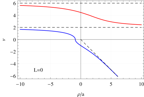
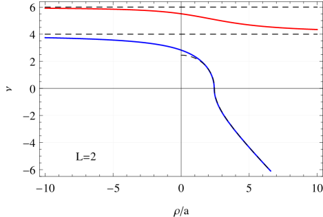
Figure 1: (Color online) The two lowest angular eigenvalue $\nu$ as a function of $\rho/a$ for $L=0$ (Upper panel) and $L=2$ (Lower panel). The asymptotic solutions are dashed. Negative $\nu$ corresponding to imaginary solution.

3.6 The Hyperradial Equation

To proceed analytically, we focus on the unitary limit, $|a|\rightarrow\infty$. In this case $\nu_{L}(\rho)=\nu_{L}$ and $\Phi(\rho,\Omega)=\Phi(\Omega)$, therefore the non-adiabatic couplings, Eq. (21), vanish and the hyperradial equation for $\mathcal{R}(\rho)/\sqrt{\rho}$ is just the Bessel equation,

$$-\frac{\partial^{2}\mathcal{R}_{n}(\rho)}{\partial\rho^{2}}+\frac{\nu_{L}^{2}-1/4}{\rho^{2}}\mathcal{R}_{n}(\rho)=\epsilon\mathcal{R}_{n}(\rho).$$ (39)

In order to calculate the trimer photoassociation, caused by $s-$ and $d$-wave operators, we have to solve the $L=0$ bound state as well as the $L=0,2$ continuum states. The needed solutions are the followings:

I. A bound state ($\epsilon<0$) with $L=0$, and $\nu_{0}\approx 1.00624i$. In this case the relevant solution is proportional to the modified Bessel function of the second kind and imaginary order, $\sqrt{\rho}K_{\nu_{0}}(\kappa\rho)$, where $\kappa=\sqrt{-\epsilon}$. At the origin, this solution behaves like $\sin(\nu\ln(\kappa\rho/2)-\gamma_{\nu})$, where $\gamma_{\nu_{0}}\approx-0.301$. Therefore regularization is needed to avoid collapse, e.g. setting $\mathcal{R}(\rho\leq\rho_{0})=0$ for some finite $\rho_{0}$. The result is the discrete Efimov spectrum,

$$\frac{\epsilon_{m}}{\epsilon_{0}}=e^{-2\pi m/|\nu_{0}|}\approx 515^{-m}.$$ (40)

The normalized wave functions are

$$\mathcal{R}^{(m)}_{B}(\rho)=N_{B}\kappa_{m}\sqrt{\rho}K_{\nu_{0}}(\kappa_{m}\rho)$$ (41)

where $N_{B}=\sqrt{2\sin\nu_{0}\pi/\nu_{0}\pi}\approx 2.730$, and

$$\frac{\kappa_{m}}{\kappa_{0}}=e^{-\pi m/|\nu_{0}|}\approx 22.7^{-m}.$$ (42)

II. Scattering state ($\epsilon>0$) with $L=0$, and $\nu_{0}\approx 1.00624i$. The solution is composed of the real part of the Bessel functions of the first and second kind of imaginary order,

$$\mathcal{R}_{s}(\rho)=\sqrt{\frac{q\rho}{2R}}\left[\sin\delta\mathrm{Re}[J_{\nu_{0}}(q\rho)]+\cos\delta\mathrm{Re}[Y_{\nu_{0}}(q\rho)]\right]$$ (43)

where $q=\sqrt{\epsilon}$ and we assume normalization in a sphere of radius $R$. The phase shift $\delta$ is to be found from the boundary condition, $\mathcal{R}_{s}(\rho_{0})=0$.

In the scattering problem, functions with higher $\nu$, corresponding to the same angular momentum $L=0$ and energy $\epsilon$, are also legitimate solutions. However, due to the orthogonality in $\Omega$, there is no overlap between these functions and the bound state, and therefore no contribution to the photoassociation transition matrix elements.

III. Scattering state ($\epsilon>0$) with $L=2$, and real $\nu_{2}$. The solutions are composed of the Bessel functions of first and second kind,

$$\mathcal{R}_{d}(\rho)=\sqrt{\frac{\pi q\rho}{R}}\left[\sin\delta_{d}J_{\nu_{2}}(q\rho)+\cos\delta_{d}Y_{\nu_{2}}(q\rho)\right]\;.$$ (44)

The phase shift $\delta_{d}$ is to be determined by the condition $\mathcal{R}_{d}(\rho_{0})=0$. The three lowest values for $\nu_{2}$ are, $\nu_{2}\approx 2.823$, $\nu_{2}^{1}\approx 5.508$ and $\nu_{2}^{2}\approx 6.449$.

4 The Transition Matrix Elements

Now that we have solved the Schroedinger equation and obtained the $L=0$ bound state wave function and the $L=0,2$ scattering wave functions, we are in a position to evaluate the transition matrix elements, in both hierarchies. For the normal hierarchy case the needed matrix elements (10) read,

$$I_{1b}^{s}=\langle\psi^{f}_{L^{\prime}}\|\sum_{j=1}^{N}r_{j}^{2}Y_{0}\|\psi^{i}_{L}\rangle,$$ (45)

for the $s-$mode transition and

$$I_{1b}^{d}=\langle\psi^{f}_{L^{\prime}}\|\sum_{j=1}^{N}r_{j}^{2}Y_{2}(\hat{r}_{j})\|\psi^{i}_{L}\rangle$$ (46)

for the $d-$mode. For the strong hierarchy case (11) the matrix element is,

$$I_{2b}=\langle\psi^{f}_{L^{\prime}}\|\sum_{i<j}^{N}\delta_{\Lambda}(\mathbf{r}_{i}-\mathbf{r}_{j})\|\psi^{i}_{L}\rangle,$$ (47)

These matrix elements are proportional to integrals of the type

$${\cal I}_{J}(\nu,m)=\int_{\rho_{0}}^{\infty}d\rho\,K_{\nu_{0}}(\kappa\rho)\rho^{m+1}\mathrm{Re}[J_{\nu}(q\rho)].$$ (48)

or ${\cal I}_{Y}(\nu,m)$ with $Y_{\nu}$ replacing $J_{\nu}$.

Taking the lower limit to zero, these integrals can be evaluated analytically,

$${\cal I}_{J}(\nu,m)\approx{\rm Re}\left[\frac{2^{m}N_{\nu_{0},\nu}^{m}}{\kappa^{m+2}}\left(\frac{q}{\kappa}\right)^{\nu}{}_{2}F_{1}\left(a,b;c;-(q/\kappa)^{2}\right)\right]$$ (49)

where ${}_{2}F_{1}$ is the hypergeometric function with parameters $a=\frac{m-\nu_{0}+\nu}{2}+1$, $b=\frac{m+\nu_{0}+\nu}{2}+1$, and $c=\nu+1$, and $N_{\nu_{0},\nu}^{m}=\Gamma(a)\Gamma(b)/\Gamma(c)$. For $q<\kappa$ this approximation amounts to an error $\Delta{\cal I}/{\cal I}\sim x_{n}^{m+2}$, where $x_{0}\approx 0.06$ is the largest zero of $K_{\nu_{0}}(x)$ and $x_{n}$ is the $n$’th root. Similar results can be obtained for ${\cal I}_{Y}$.

4.1 Transition matrix elements in the normal hierarchy case

The $r^{2}$ matrix element. The $r^{2}$ operator connects the $L=0$ bound state to the $L=0$ scattering state. We note that $\sum_{j}r_{j}^{2}=\rho^{2}+3R_{CM}^{2}$ where $\mathbf{R}_{CM}$ is the center of mass coordinate. As the CM cannot induce inelastic transition, the matrix element is reduced into the hyperradial integral

$$I_{s}(\kappa,q)=\int_{0}^{\infty}d\rho\mathcal{R}_{B}^{*}(\rho)\rho^{2}\mathcal{R}_{s}(\rho).$$ (50)

Substituting Eqs. (41) and (43) into (50), we get

$$I_{s}(\kappa,q)=\sqrt{\frac{q}{2R}}N_{B}\kappa\left[I_{J}(\nu_{0},2)\sin\delta+I_{Y}(\nu_{0},2)\cos\delta\right].$$ (51)

This integral depends on the momentum of the bound state $\kappa$ and the scattering state $q$. The maximal value of $I_{s}(\kappa,q)$ is obtained when $q\approx\kappa/2$. For higher Efimov states, this integral scales such as

$$p^{5/2}I_{s}(\kappa_{m},qp)=I_{s}(\kappa_{0},q)$$

where $p=\kappa_{m}/\kappa_{0}=22.7^{-m}$,

It should be noted that (50) leads to an oscillatory log-periodic response function, see discussion in [17]. At threshold, the matrix element (50) gets a particularly simple form which can be well approximated by [17]

$$I_{s}(\kappa,q)\approx C\kappa^{-3}\sqrt{q}\left(1+\frac{B_{3}}{2}\cos(2|\nu_{0}|\ln\frac{q}{\kappa})\right)$$ (52)

where $C$ is a constant that contains the normalization factors, and $B_{3}\approx 8.475\%$ is the normalized amplitude of these oscillations. These oscillations modulate the matrix element all the way to the high energy tail. Whereas log periodic oscillations at the high energy tail appear in all partial waves [28], at threshold the oscillations appear only in this $s$-wave transition.

The quadrupole matrix element. The quadrupole operator, $\sum_{j}r_{j}^{2}Y_{2}^{M}(\hat{r}_{j})$ connects the $L=0$ bound state with $L=2$ scattering states. Using $\mathbf{r}_{j}=\mathbf{R}_{CM}-\sqrt{\frac{2}{3}}\mathbf{y}_{j}$ and working in center of mass coordinate system, this operator reads $\frac{2}{3}\sum_{j}y_{j}^{2}Y_{2}^{M}(\hat{y}_{j})$. Setting $y_{j}^{2}=\rho^{2}\cos^{2}\alpha_{j}$, the reduced matrix element can be written as

$$\langle\psi_{B}\|\sum_{j}r_{j}^{2}Y_{2}\|\psi_{d}\rangle=\frac{3}{2}\sqrt{5}I_{\rho}I_{\Omega}.$$ (53)

Here the hyperradial integral $I_{\rho}$ is

$$I_{\rho}=\int_{0}^{\infty}d\rho\mathcal{R}_{B}^{*}(\rho)\rho^{2}\mathcal{R}_{d}(\rho).$$ (54)

Substituting Eqs. (41) and (44) into (54), we get an expression similar to (51),

$$I_{\rho}(\kappa,q)=\sqrt{\frac{\pi q}{R}}N_{B}\kappa\left[I_{J}(\nu_{2},2)\sin\delta_{d}+I_{Y}(\nu_{2},2)\cos\delta_{d}\right].$$ (55)

The hyperangular integral $I_{\Omega}$, reads

$$I_{\Omega}=\int d\Omega\Phi_{f}(\Omega)\sum_{j}\cos^{2}\alpha_{j}Y_{20}(\hat{y}_{j})\Phi_{i}(\Omega).$$ (56)

To evaluate this integral, the hyperangular wave function, written in mixed coordinate systems,

$$\Phi_{L}(\Omega)=\sum_{i}P_{\nu}^{L}(\alpha_{i})Y_{0L}(\hat{x}_{i},\hat{y}_{i})/\sin 2\alpha_{i}$$

is to be integrated in a single coordinate system. Transforming to body-fixed coordinate system and integrating over the Euler angles, the integral over the 5 angles ($\alpha_{1},\hat{x}_{1},\hat{y}_{1}$) is transformed into an integral over ($\alpha_{1},\gamma_{1}$) [30], that is evaluated numerically. See B for details. For the lowest $\nu_{2}$ the integral yields $I_{\Omega}\approx 0.368.$ For the next two $\nu_{2}^{i}$’s the integrals are respectively $0.023$ and $6.9\times 10^{-4}$, therefore these modes give negligible contribution to the reaction rates.

Here as in the previous case, the hyperradial integral $I_{\rho}$ leads to log-periodic oscillations in the high energy tail [17].

Relative importance. The relative contribution of the $s,d$ modes to the trimer formation is displayed in Fig. 2, where the last term in parenthesis on the rhs of (10) is presented normalized, along with the $s$ and $d$ components. Similarly to the dimer formation case [10], the $s$-wave association is peaked around $q\cong\kappa/2$, while the $d$-wave association is peaked around $q\cong\kappa$.

In case of large but finite scattering length, the eigenvalue of the hyperangular equation, (37) and (LABEL:l2), depends on $\rho$ and therefore the hyperradial equation (20) is to be solved numerically. In addition, the non-adiabatic couplings (21) must be considered. The numerical results for finite $a$ are also shown in Fig. 2 for $\kappa a=-100$ and $\kappa a=-50$. From the figure it can be seen that the $|a|\longrightarrow\infty$ limit is well reproduced if $\kappa|a|>100$.

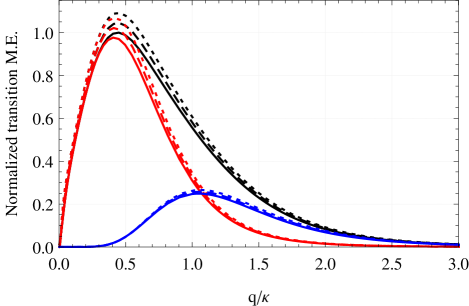
Figure 2: (Color online) One-body current: The transition matrix element $I_{1b}^{2}$, as a function of the relative momentum $q/\kappa$, normalized to 1 for the maximum value at $|a|=\infty$ The two modes are presented - $r^{2}$ (red, peaked around $q=\kappa/2$), and quadrupole (blue, peaked around $q=\kappa$), with their sum (black). Shown are the results for the unitary point (solid lines) and for finite scattering length, $\kappa a=-100$ (dotted lines) and $\kappa a=-50$ (dashed lines).

4.2 Transition matrix elements in the strong hierarchy case

Moving now to study the two-body current, there is no center of mass contribution, and the transition operator is a scalar exciting an $L=0$ bound state into an $L=0$ scattering state. The transition matrix element is given by,

$$I_{2b}=\langle\psi_{B}|\sum_{i<j}\delta_{\Lambda}(\mathbf{r}_{i}-\mathbf{r}_{j})|\psi_{i}\rangle=\frac{3}{\sqrt{8}}\langle\psi_{B}|\delta_{\Lambda}(\mathbf{x})|\psi_{i}\rangle\;.$$ (57)

Assuming a simple regularization, $\delta_{\Lambda}(\mathbf{x})=3\Lambda^{3}\Theta(1-\Lambda x)/4\pi$, this matrix element can be calculated,

$$\eqalign{I_{2b}=&\frac{9\Lambda^{2}}{64\pi}N_{B}N_{i}^{2}\kappa\sqrt{\frac{q}{R}}|\sin(\nu_{0}\pi/2)|^{2}\times\\ &\left[I_{J}(\nu_{0},-1)\sin\delta+I_{Y}(\nu_{0},-1)\cos\delta\right].}$$ (58)

To renormalize the transition matrix element and remove the cutoff dependence we turn to the dimer photoassociation [10]. In the zero range approximation the dimer $s$-wave continuum wave function is just $\psi_{i}=\sqrt{2/R}\sin(qr+\delta)/r$, and the corresponding bound state wave function is $\psi_{B}=\sqrt{2\kappa}e^{-\kappa r}/r$. Consequently the transition matrix element due to the 2-body process is

$$\eqalign{I_{2b,d}=&\langle\psi_{B}|\delta_{\Lambda}(\mathbf{r})|\psi_{i}\rangle=\Lambda^{3}\frac{6}{4\pi}\sqrt{\frac{\kappa}{R}}\biggl{(}\frac{q\cos\delta+\kappa\sin\delta}{q^{2}+\kappa^{2}}\\ &-e^{-\kappa/\Lambda}\frac{q\cos(\delta+q/\Lambda)+\kappa\sin(\delta+q/\Lambda)}{q^{2}+\kappa^{2}}\biggr{)}}$$ (59)

which for large values of $\Lambda$ can be approximated as

$$I_{2b,d}=\Lambda^{2}\frac{6}{4\pi}\sqrt{\frac{\kappa}{R}}\sin\delta+O(\Lambda)$$ (60)

Comparing this result to (58), one can see that the cutoff dependence of the 2-body current operator, $L_{2}=L_{2}(\Lambda)$ in (11), can be fixed by dimer photoassociation experiments such that the trimer photoassociation rate is a prediction of this theory.

As an alternative approach to fix $L_{2}(\Lambda)$, we can study the shift of the dimer binding energy due to a small change in the static magnetic field. On one hand,

$$\delta E_{2}=\langle\psi_{B}|H_{I}^{(2b)}|\psi_{B}\rangle=\frac{L_{2}}{\Lambda^{3}}\frac{3}{\pi a}\langle s_{0}\rangle\Lambda^{2}\delta B+O(\Lambda).$$ (61)

On the other hand, in the vicinity of a Feshbach resonance

$$a(B)\approx a_{bg}\frac{\Delta}{B-B_{0}},$$ (62)

where $a_{bg}$ is the background scattering length, $\Delta$ is the resonance width and $B_{0}$ its position, therefore

$$\delta E_{2}=\frac{dE}{da}\frac{da}{dB}\delta B=\frac{2\hbar^{2}}{maa_{bg}\Delta}\delta B.$$ (63)

Comparing (61) and (63), $L_{2}(\Lambda)$ can be determined,

$$L_{2}(\Lambda)=\frac{2\pi}{3}\frac{\hbar^{2}}{ma_{bg}\Delta}\frac{1}{\langle s_{0}\rangle}\Lambda.$$ (64)

In Fig. (3) the two-body transition matrix element is shown as a function of the relative momentum $q/\kappa$. The validity of the approximation deriving (49) is also checked by evaluating the integral numerically, starting from $\rho_{0}$. It can be seen that while for the low momentum regime this approximation is excellent, for the high momentum tail it deviates from the exact result. Numerical results for finite $a$ are also shown in Fig. (3). For $\kappa a=-100$ and $\kappa a=-50$, we see no significant difference comparing to the unitary point.

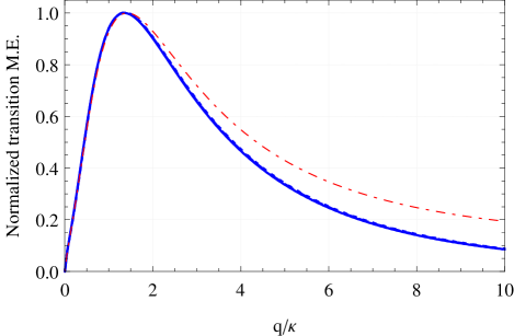
Figure 3: (Color online) Two-body current: The transition matrix element $I_{2b}^{2}$, as a function of the relative momentum $q/\kappa$, normalized to 1 for the maximum value at $|a|=\infty$. For the unitary point the exact result is shown (blue solid line), as well as the approximation of (58) (red dot-dashed line). Also shown are results for finite scattering length, $\kappa a=-100$ (dotted lines) and $\kappa a=-50$ (dashed lines).

5 Transition rates

To evaluate the trimer photoassociation rate (1), we have to average on the initial states $\bar{\sum_{i}}$ and to sum over the final states $\sum_{f}$. The initial three-body state $|i\rangle=|qLMl_{x}l_{y}\rangle$ describes three atoms in the continuum with relative momentum $q$ and angular momenta $L,M,l_{x},l_{y}$. The average on these states takes the form

$$\bar{\sum_{i}}=\frac{1}{\pi}\int_{0}^{\infty}dq\sum_{[K]}\left(R+\frac{d\delta}{dq}\right)P_{[K]}(q)\;,$$ (65)

where $P_{[K]}(q)$ is the probability of finding an atomic trio with quantum numbers $[K]=\{KLMl_{x}l_{y}\}$ and momentum $q$. For system in thermal equilibrium with temperature $T$ higher than the condensation temperature,

$$P_{[K]}(q)=\frac{1}{\mathcal{Z}}e^{-\frac{\hbar^{2}q^{2}}{2mk_{B}T}},$$

where $\mathcal{Z}$ is the partition function, $k_{B}$ is the Boltzmann constant and $T$ is the temperature.

The sum $\sum_{f}$ contains all possible trimer quantum numbers and all possible photons weighted by the emission function,

$$\sum_{f}=\sum_{\mathbf{k},\zeta}\sum_{L^{\prime},M^{\prime}}({1+N_{\mathbf{k}\zeta}}),$$ (66)

where $N_{\mathbf{k}\zeta}$ is the number of photons with momentum $\mathbf{k}$ and polarization $\zeta$ in the final state. The stimulating rf radiation is a narrow distribution centered at some $\mathbf{k}_{\mathrm{rf}}$. Therefore $N_{\mathbf{k}\zeta}\approx N_{\mathbf{k}_{\mathrm{rf}}\zeta_{\mathrm{rf}}}\delta_{\mathbf{k},\mathbf{k}_{\mathrm{rf}}}\delta_{\zeta,\zeta_{\mathrm{rf}}}$, where $\mathbf{k}_{\mathrm{rf}}$ is the momentum of the stimulating rf field and $\zeta_{\mathrm{rf}}$ is its polarization.

5.1 Transition rate in the normal hierarchy case

Substituting (10), (65) and (66) into Fermi’s golden rule (1), the trimer formation rate in the normal hierarchy case is given by

$$r^{1b}_{i\rightarrow f}=\frac{4\pi\mu_{1}^{2}R}{\epsilon_{0}c^{6}}\frac{m}{\hbar^{2}}n_{\mathrm{rf}}\left|\left\langle s_{0}\right\rangle\right|^{2}\eta^{2}\frac{\omega^{5}}{q}P(q)\left(\frac{I_{s}^{2}}{6^{2}}+\frac{5I_{d}^{2}}{15^{2}}\right).$$ (67)

where $n_{\mathrm{rf}}=N_{\mathbf{k}_{\mathrm{rf}},\zeta_{\mathrm{rf}}}/\Omega$ is the photon density of the rf field. The relative momentum $q$ is connected to the photon energy through energy conservation $\hbar^{2}q^{2}/2m=-E_{3}+\hbar\omega$, where $E_{3}$ is the trimer binding energy.

The relative importance of the $s,d$ modes shifts with temperature. This point is demonstrated in Fig. 4, where the $s,d$ rates to the trimer photoassociation, at the unitary point $|a|=\infty$ and for large but finite scattering length are presented for $k_{B}T=E_{3}$ and $k_{B}T=0.2E_{3}$. The importance of the $d$ mode grows with the ratio $k_{B}T/E_{3}$. Therefore we can conclude that for small $k_{B}T/E_{3}$ values, the photoassociation is an $s$-wave process while for large values the two modes have similar importance. In addition, oscillations in the response can be clearly seen at the low frequency regime. These oscillations result form the log-periodic structure of the matrix element [17]. At higher temperature these oscillations are stronger while at lower temperatures this manifestation of the Efimov effect is suppressed by the Boltzmann factor. The amplitude of the oscillations is larger for finite scattering length than at the unitary point.

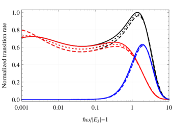
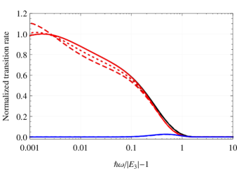
Figure 4: (Color online) One-body current: The normalized trimer photoassociation rate as a function of the rf photon frequency, for different temperatures and scattering lengths. The total (black), the $r^{2}$ (red, low energy peak) and the quadrupole (blue) rates are presented, for temperature of $k_{B}T=E_{3}$ (upper panel) and $k_{B}T=0.2E_{3}$ (lower panel). Shown are results for the unitary point (solid lines) and for finite scattering length, $\kappa a=-100$ (dotted lines) and $\kappa a=-50$ (dashed lines).

5.2 Transition rate in the strong hierarchy case

For the strong hierarchy case, the trimer formation rate is given by

$$r^{2b,t}_{i\rightarrow f}=\frac{L_{2}^{2}}{\Lambda^{6}}\frac{4mR}{\hbar^{2}c^{2}\epsilon_{0}}n_{\mathrm{rf}}\left|\left\langle s_{0}\right\rangle\right|^{2}\eta^{2}\frac{\omega}{q}P_{t}(q)I_{2b,t}^{2}.$$ (68)

Here we have added the subscript “$t$” to $P(q),I_{2b}$ to stress these are trimer related quantities. The corresponding dimer formation rate for this case is given by

$$r^{2b,d}_{i\rightarrow f}=\frac{L_{2}^{2}}{\Lambda^{6}}\frac{2mR}{\hbar^{2}c^{2}\epsilon_{0}}n_{\mathrm{rf}}\left|\left\langle s_{0}\right\rangle\right|^{2}\eta^{2}\frac{\omega}{q}P_{d}(q)I_{2b,d}^{2},$$ (69)

where $P_{d}(q)$ is the probability for a pair of particles to be in $L=0$ state with momentum $q$. Comparing these two results and using Eqs. (60),(64) we finally obtain

$$\frac{r^{2b,t}_{i\rightarrow f}}{r^{2b,d}_{i\rightarrow f}}=2\frac{P_{t}(q)}{P_{d}(q)}\frac{I_{2b,t}^{2}}{I_{2b,d}^{2}}$$ (70)

and

$${r^{2b,d}_{i\rightarrow f}}=\left(\frac{\hbar^{2}}{ma_{bg}\Delta}\right)^{2}\frac{2m}{\hbar^{2}c^{2}\epsilon_{0}}n_{\mathrm{rf}}\eta^{2}\frac{\omega}{q}P_{d}(q)\kappa\sin^{2}\delta(q)$$ (71)

One should note that these results are independent of the cutoff parameter $\Lambda$. The dependence of the rates on the normalization radius $R$ enters through the probability $P_{d/t}(q)$.

The trimer transition rate for the strong hierarchy case is shown for $k_{B}T=E_{3}$ in Fig. 5. Here as in the normal hierarchy case, log periodic oscillations are visible. For finite scattering length they are amplified. Since there is only a single channel here, the low temperature behavior is similar to the high temperature, and therefore not shown.

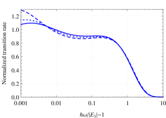
Figure 5: (Color online) Two-body current: The normalized trimer photoassociation rate as a function of the rf photon frequency. Shown are the results for $k_{B}T=E_{3}$ at the unitary point (solid lines) and at finite scattering lengths, $\kappa a=-100$ (dotted line) and $\kappa a=-50$ (dashed line).

6 Experimental results

In this section we apply our theory to the photoassociation of ultracold ⁷Li atoms, and fit it to the experimental results of the Bar-Ilan group [9].

In this experiment, a gas of ⁷Li atoms on the $|F=1,m_{F}=0\rangle$ state was cooled down to $T\approx 1.5\mu K$, with mean density of about $10^{12}\mathrm{cm}^{-3}$. A static magnetic field was applied in the vicinity of a Feshbach resonance at $\sim$894 G. Then an rf field was turned on for $\sim 1$ msec. The magnetic component of the rf field was parallel to the static magnetic field, therefore $\eta=1$. The number of atoms remains in the trap was measured as function of the rf frequency.

The scattering length in this experiment is positive, therefore both dimers and trimers can be associated by the rf field. The experimental signal for photoassociation is particle loss from the trap. In both cases three particles are lost for each associated molecule. Internal collisions break the trimer into a deeply bound dimer and an atom, both carry high kinetic energy and therefore escape the trap. The dimer collides with a third atom and decays to a deeper bound state, and in the process enough energy is released such that both atom and dimer escape the trap.

To connect the photoassociation rate to the measured quantity we integrate the population evolution equation

$$\dot{N}=-3r^{2b,d}_{i\rightarrow f}\frac{N^{2}}{2}-3r^{2b,t}_{i\rightarrow f}\frac{N^{3}}{3!}\;,$$ (72)

where the dimer (trimer) photoassociation rate is multiplied by the numbers of pairs (trios) is the system. Since this experiment is clearly in the strong hierarchy regime, we use Eqs. (68) and (69) for the transition rates.

To fix the value of $L_{2}$ we use Eq. (64), where the relevant Feshbach resonance parameters are $a_{bg}\approx-18.24a_{0}$ and $\Delta\approx-237.8$G [29]. Doing so, see Eqs. (70),(71), the transition rate is independent of $\Lambda$ and also of the effective charge $\langle s_{0}\rangle$.

The photon density is connected to the amplitude of the oscillating magnetic field $B_{\mathrm{rf}}$ through $n_{\mathrm{rf}}=B_{\mathrm{rf}}^{2}/2\mu_{0}\hbar\omega$, where $\mu_{0}$ is the vacuum permeability.

Due to strong rf field there is power broadening which blurs the fine structure of the transition rate. To account for this effect we convolute the transition rates with a Gaussian,

$$r_{i\rightarrow f}(\omega)=\frac{1}{\sqrt{2\pi}\sigma}\int d\omega^{\prime}r_{i\rightarrow f}(\omega^{\prime})e^{-\frac{(\omega-\omega^{\prime})^{2}}{2\sigma^{2}}},$$ (73)

where the Gaussian width $\sigma$ was fitted to the experimental results.

The fitting parameters are shown in Table 1.

Table 1: The fitting parameters for the ⁷Li photoassociation experimental results. Here $n$ is the number density and $\sigma$ is the broadening width.

• Case	$a(a_{0})$	$n(10^{12}\mathrm{cm}^{-3})$	$B_{\mathrm{rf}}$ (G)	$E_{3}/h$ (MHz)	$\sigma$ (kHz)
  a	806	1.3	0.6	0.93	25
  b	629	1.0	0.52	1.45	20

Our theory for photoassociation of ⁷Li ultracold atoms, as well as the experimental results of Ref. [9] are shown in Fig. 6. To distinguish the power broadening effect the results without broadening are also shown in dotted curve. Our theory agrees well with the experimental results, and the fitting parameters are within the experimental uncertainty. However, the experimental resolution limits the ability to identify fine details of the association process.

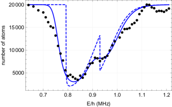
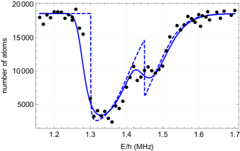
Figure 6: (Color online) The number of ⁷Li atoms remaining in the trap after photoassociation experiment, as function of the rf frequency. Shown are the experimental results from Ref. [9], for $a/a_{0}\approx 810$ (upper plot) and $a/a_{0}\approx 627$ (lower plot), as well as our fitting results. To distinguish the power broadening effect the results without broadening are also shown in dotted curve.

7 Conclusion

To conclude, we have applied the multipole expansion to study universal trimer photoassociation. One-body and two-body current were explored. For normal hierarchy case, where the one-body current dominates, the two leading $s-$ and $d-$ modes are studied and their relative contribution is shown to vary with temperature. In ultracold atoms, and other strong hierarchy systems, the relevant operator is found to be the two-body current. The log-periodic oscillations which modulate the cross section in both scenarios is found to be amplified for finite scattering length compared to the unitary point. We apply out theory to ⁷Li ultracold atoms photoassociation and show nice fit with the available experimental results.

Appendix A Raynal-Revai coefficients

Our calculation of the projector operator (LABEL:Rot), provides an explicit formula for the $l_{x}=0$ or $l_{y}=0$ Raynal-Revai coefficients $\langle l_{x}l_{y}|l^{\prime}_{x}l^{\prime}_{y}\rangle_{KL}$ [24], defined by

$$\mathcal{Y}^{KLM}_{l_{x}l_{y}}(\Omega_{i})=\sum_{l^{\prime}_{x}l^{\prime}_{y}}\langle l_{x}l_{y}|l^{\prime}_{x}l^{\prime}_{y}\rangle_{KL}\mathcal{Y}^{KLM}_{l^{\prime}_{x}l^{\prime}_{y}}(\Omega_{j}).$$ (74)

Using the orthogonality of the hyperspherical harmonics we get,

$$\langle l_{x}l_{y}|l^{\prime}_{x}l^{\prime}_{y}\rangle_{KL}=\frac{R_{ij}^{(l_{x}l_{y})(l_{x}^{\prime}l_{y}^{\prime})}[\varphi^{K}_{l^{\prime}_{x}l^{\prime}_{y}}(\alpha_{j})](\alpha_{i})}{\varphi^{K}_{l_{x}l_{y}}(\alpha_{i})}.$$ (75)

Putting $l_{x}=0,l_{y}=L$ and $\alpha_{i}=0$,

$$\eqalign{\langle 0L|l^{\prime}_{x}l^{\prime}_{y}\rangle_{KL}=(\mp)^{l^{\prime}_{x}}\sqrt{(2l^{\prime}_{x}+1)(2l^{\prime}_{y}+1)}\times\cr\left(\begin{array}[]{ccc}l_{x}^{\prime}&l_{y}^{\prime}&L\\ 0&0&0\end{array}\right)\frac{\varphi^{K}_{l^{\prime}_{x}l^{\prime}_{y}}(\pi/3)}{\varphi^{K}_{0L}(0)}.}$$ (76)

Similar calculation for $l_{x}=L,l_{y}=0$ and $\alpha_{i}=\pi/2$ gives

$$\eqalign{\langle L0|l^{\prime}_{x}l^{\prime}_{y}\rangle_{KL}=(\pm)^{l^{\prime}_{y}}\sqrt{(2l^{\prime}_{x}+1)(2l^{\prime}_{y}+1)}\times\cr\left(\begin{array}[]{ccc}l_{x}^{\prime}&l_{y}^{\prime}&L\\ 0&0&0\end{array}\right)\frac{\varphi^{K}_{l^{\prime}_{x}l^{\prime}_{y}}(\pi/6)}{\varphi^{K}_{L0}(\pi/2)}.}$$ (77)

Appendix B The hyperangular integrals

The wave function is written as sum of Faddeev components, each in different coordinate set,

$$\Phi_{\nu}^{L}(\Omega)=\frac{1}{\sqrt{4\pi}}\sum_{i=1}^{3}Y_{L0}(\hat{y}_{i})P_{\nu}^{L}(\alpha_{i})/\sin 2\alpha_{i}.$$ (78)

Our aim is to evaluate the hyperangular integral,

$$I_{\Omega}=\int d\Omega_{1}\Phi^{0*}_{\nu}(\Omega)\left(\sum_{j}Y_{20}(\hat{y}_{j})\cos^{2}\alpha_{j}\right)\Phi^{2}_{\nu^{\prime}}(\Omega)$$ (79)

Due to symmetry, one of the sums, say over $j$, can be dropped giving a factor of 3. The integral (79) can be further simplified utilizing the body-fixed coordinate system [30]. Consider the two body-fixed vectors $\mathbf{x}_{10}$ and $\mathbf{y}_{10}$ such that $\hat{x}_{10}\cdot\hat{y}_{10}=\gamma_{i}$. The transformation from the body-fixed to system to the laboratory system is given through the relation

$$Y_{lm}(\hat{y}_{i})=\sum_{\mu}D_{\mu m}^{l}(\omega)Y_{l\mu}(\hat{y}_{i0}),$$ (80)

where $D_{\mu m}^{l}(\omega)$ is the Wigner D-matrix, and the rotation $\omega$ is the set of 3 Euler angles. Applying this transformation, for fixed $\alpha_{i}$,

$$\eqalign{\frac{1}{4\pi}&\int d\hat{x}_{i}\int d\hat{y}_{i}Y_{lm}^{*}(\hat{y}_{i})Y_{l^{\prime}m^{\prime}}(\hat{y}_{j})=\\ \int d\gamma_{i}&\sum_{\mu,\mu^{\prime}}Y_{l\mu}^{*}(\hat{y}_{i0})Y_{l^{\prime}\mu^{\prime}}(\hat{y}_{j0})\int d\omega D_{\mu m}^{l*}(\omega)D_{\mu^{\prime}m^{\prime}}^{l^{\prime}}(\omega)}.$$

Now one can utilize the orthogonality of the Wigner D-matrix,

$$\int d\omega D_{\mu m}^{l*}(\omega)D_{\mu^{\prime}m^{\prime}}^{l^{\prime}}(\omega)=\frac{8\pi^{2}}{2l+1}\delta_{l,l^{\prime}}\delta_{\mu,\mu^{\prime}}\delta_{m,m^{\prime}}$$ (81)

and the addition theorem

$$\sum_{\mu}Y_{l\mu}^{*}(\hat{y}_{i0})Y_{l\mu}(\hat{y}_{j0})=\frac{2l+1}{4\pi}P_{l}(\gamma_{ij})$$ (82)

where $P_{l}(\gamma_{ij})$ is the Legendre polynomials and $\gamma_{ij}=\hat{y}_{i0}\cdot\hat{y}_{j0}$. Choosing $\mathbf{x}_{i0}=\rho\sin(\alpha_{i})\hat{z}$ and $\mathbf{y}_{i0}=\rho\cos(\alpha_{i})(\sqrt{1-\gamma_{i}^{2}}\hat{x}+\gamma_{i}\hat{z})$,

$$\gamma_{ij}(\alpha_{i},\gamma_{i})=-\frac{\cos\alpha_{i}\pm\sqrt{3}\gamma_{i}\cos\alpha_{i}}{\sqrt{1+2\sin^{2}\alpha_{i}\pm\sqrt{3}\gamma_{i}\sin 2\alpha_{i}}}.$$ (83)

Finally,

$$\eqalign{I_{\Omega}=\frac{3}{4\sqrt{\pi}}\int_{-1}^{1}d\gamma_{1}\int_{0}^{\pi/2}d\alpha_{1}\sin^{2}\alpha_{1}\cos^{4}\alpha_{1}\times\\ \sum_{i,k}P_{2}(\gamma_{1k})\frac{P_{\nu}^{0*}(\alpha_{i})}{\sin 2\alpha_{i}}\frac{P_{\nu^{\prime}}^{2}(\alpha_{k})}{\sin 2\alpha_{k}},}$$ (84)

where $\alpha_{i}=\alpha_{i}(\alpha_{1},\gamma_{1})$ is given by (14).

References

References

• [1] E. Braaten and H.W. Hammer 2006 Phys. Rep. 428 259-390
• [2] C. Chin, R. Grimm, P. Julienne, and E. Tiesinga 2010 Rev. Mod. Phys. 82 1225-86
• [3] V. Efimov 1970 Phys. Lett. B 33 563-4
• [4] V. N. Efimov 1970 Sov. J. Nucl. Phys. 12 589
• [5] F. Ferlaino, A. Zenesini, M. Berninger, B. Huang, H.-C. Nägerl, and R. Grimm 2011 Few-Body Syst. 51 113-33
• [6] S. T. Thompson, E. Hodby, and C. E. Wieman 2005 Phys. Rev. Lett. 95 190404
• [7] Th. Lompe, T. Ottenstein, F. Serwane, A. Wenz, G. Zürn, and S. Jochim 2010 Science 330 940-944
• [8] S. Nakajima, M. Horikoshi, T. Mukaiyama, P. Naidon, and M. Ueda 2011 Phys. Rev. Lett. 106 143201
• [9] O. Machtey, Z. Shotan, N. Gross, and L. Khaykovich 2012 Phys. Rev. Lett. 108 210406
• [10] B. Bazak, E. Liverts, and N. Barnea 2012 Phys. Rev. A 86 043611
• [11] C. Chin and P.S. Julienne 2005 Phys. Rev. A 71 012713
• [12] J. F. Bertelsen and K. Mølmer 2006 Phys. Rev. A 73 013811
• [13] T. M. Hanna, T. Köhler, and K. Burnett 2007 Phys. Rev. A 75 013606
• [14] C. Klempt, T. Henninger, O. Topic, M. Scherer, L. Kattner, E. Tiemann, W. Ertmer, and J. J. Arlt 2008 Phys. Rev. A 78 061602
• [15] T. V. Tscherbul and S. T. Rittenhouse 2011 Phys. Rev. A 84 062706
• [16] E. Liverts, B. Bazak, and N. Barnea 2012 Phys. Rev. Lett. 108 112501
• [17] B. Bazak and N. Barnea 2014 Phys. Rev. A 89 030501(R)
• [18] D. B. Kaplan 2005 arXiv:nucl-th/0510023 [nucl-th]
• [19] Y. H. Song, R. Lazauskas, and T. S. Park 2009 Phys. Rev. C 79 064002
• [20] J. Macek 1968 J. Phys. B: At. Mol. Phys. 1 831
• [21] B. D. Esry, C. H. Greene, and J. P. Burke 1999 Phys. Rev. Lett. 83 1751-54
• [22] J. Avery 1993 J. Phys. Chem. 97 2406-12
• [23] A. Cobis, D. V. Fedorov, and A. S. Jensen 1997 Phys. Rev. Lett. 79 2411-4
• [24] J. Raynal and J. Revai 1970 Nuovo Cimento A 68 612-22
• [25] E. Nielsen, D. V. Fedorov, A. S. Jensen, and E. Garrido 2001 Phys. Rep., 347 373-459
• [26] D. V. Fedorov and A. S. Jensen 2002 Nucl. Phys. A 697 783-801
• [27] D. V. Fedorov and A. S. Jensen 2001 J. Phys. A: Math. Gen. 34 6003
• [28] E. Braaten, D. Kang, and L. Platter 2011 Phys. Rev. Lett., 106 153005
• [29] N. Gross, Z. Shotan, O. Machtey, S. Kokkelmans, and L. Khaykovich 2011 C. R. Phys. 12 4-12
• [30] N. Barnea, V. D. Efros, W. Leidemann, and G. Orlandini 2004 Few-Body Systems, 35 155-67