Phase transition in multicomponent field theory at finite temperature

Abstract:

Nuclear matter at finite temperature and barion density exhibits several phase transitions that could happen at the early stages of the Universe evolution and could be realized in heavy-ion or hadron-hadron collisions. Microscopic description of phase transitions is notoriously difficult because of the absence of small parameters. Here we present a general approach allowing to treat situations, when there are no small parameters. The approach is based on optimized perturbation theory and self-similar approximation theory. It allows, starting with divergent perturbation series in powers of an asymptotically small parameter, to construct expressions extrapolating asymptotic series to arbitrary values of the parameter, including its infinite limit. Examples of such approximants are: right root approximants, left root approximants, continued root approximants, exponential approximants, and factor approximants. The approach is illustrated by the phase transition of gauge symmetry breaking in a multicomponent field theory. The found critical indices are in very good agreement with Monte Carlo simulations as well as with complicated methods of Padé-Borel summation, while our approach is much simpler. The nice feature of the approach is that it gives exact values for the cases where exact solutions are known.

1 Introduction

Varying temperature and baryon density, it is possible to realize several different phases of nuclear matter. A qualitative phase portrait of admissible phases, on temperature-baryon density plane, is shown in Fig. 1, where $\rho_{0}=0.167$ fm^-3 is the normal baryon density (e.g., [1]). The variation of temperature and baryon density can be achieved in hadron-hadron and heavy-ion collisions. The corresponding values of these thermodynamic variables could also exist at the early stages of the Universe evolution or in the cores of neutron stars. There can occur phase transitions of first order, second order, as well as crossovers [2-4].

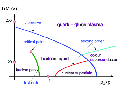
Figure 1: Figure 1: A qualitative phase portrait of admissible phases, on temperature-baryon density plane.

Phase transitions are known to be difficult for description because of the absence of small parameters in the transition region. This especially concerns the description of phase transitions in microscopic theory, where calculations are possible only by resorting to a kind of perturbation theory. However, perturbation theory usually results in divergent series that, in the best case, have meaning in the limit of asymptotically small parameters, while the physical parameters could be rather large, or even infinite. The notorious question is: How it would be possible to extract information from perturbative series, derived for asymptotically small parameters, for the values of finite and large parameters?

There exist methods for effective summation of divergent series, such as Padé summation [5] and Borel summation [6]. However, the former exhibits a number of deficiencies, including the appearance of spurious poles, while the second is quite complicated and requiring the knowledge of large-order terms in power law expansions. Both these methods not always are applicable, as is discussed in [7].

In the present report, we describe an original approach to treating divergent perturbative series, extracting from them meaningful answers, providing good accuracy, with being much simpler and more general than Padé-Borel summation. We illustrate the approach by the example of a phase transition in multicomponent field theory at finite temperature.

2 Optimized perturbation theory

The first step of the approach is optimized perturbation theory, based on the definition of control functions reorganizing divergent series to convergent ones. The optimized perturbation theory was advanced in 1973, in Thesis [8], submitted for publication in 1974, and published [9,10] in 1976. The power of this method was illustrated by treating some anharmonic models and strongly anharmonic quantum crystals [8-18]. Later this theory has been applied to numerous models, under different guises and under different names, such as modified perturbation theory, variational perturbation theory, renormalized perturbation theory, oscillator representation, delta expansion, optimized expansion, nonperturbative expansion, and so on (e.g., [19-24]). All these works have used the variants of the same idea [8-18] of introducing control functions renormalizing divergent perturbative series into convergent series. In this section, we briefly delineate the idea of optimized perturbation theory, as advanced in [8-18] and reviewed in [25,26].

Suppose we are interested in finding a function $f(x)$ satisfying a complicated equation that cannot be solved exactly, but can be treated only by a kind of perturbation theory. To explain the main idea, we consider here, for simplicity, a real function of a real variable. A generalization to complex functions and variables is straightforward.

Let perturbation theory give a divergent perturbative sequence $\{f_{k}(x)\}$, with $k=0,1,2,\ldots$ being an approximation-order index. The basic idea of optimized perturbation theory is to introduce a set $\{u_{k}(x)\}$ of control functions that would allow us to reorganize the divergent perturbative sequence $\{f_{k}(x)\}$ into a convergent sequence $\{F_{k}(x,u_{k})\}$, where $u_{k}=u_{k}(x)$. A sequence is convergent if and only if it satisfies the Cauchy criterion: For each positive $\epsilon$, there exists an order $k_{\epsilon}$, such that

$$|F_{k+p}(x,u_{k+p})-F_{k}(x,u_{k})|<\varepsilon\;,$$ (1)

for $k>k_{\epsilon}$ and any positive $p=0,1,2,\ldots$.

Control functions can be introduced in several ways, three of which are the most common: (i) through initial conditions, (ii) through variable changes, and (iii) through functional transformations.

Introduction of control functions through initial conditions

The simplest illustration of this way is when the sought function $f(x)$ is a solution of a functional equation

$${\cal E}[f(x)]=0\;.$$ (2)

Then, starting with an initial approximation $F_{0}(x,u)$, including a control function $u$, it is admissible to represent the functional equation (2) as an iterative procedure

$$F_{k}(x,u_{k})=F_{k-1}(x,u_{k-1})+{\cal E}[F_{k-1}(x,u_{k-1})]\;.$$ (3)

As a rule, physical systems are characterized by their Hamiltonians, or Lagrangians. Say, $H$ is a Hamiltonian of a complicated system that can be treated only by means of perturbation theory. Taking for the zero approximation a simple Hamiltonian $H_{0}(u)$, containing control functions, one can rewrite the system Hamiltonian as

$$H=H_{0}(u)+[H-H_{0}(u)]\;.$$ (4)

Then, by perturbation theory with respect to the difference $(H-H_{0})$, one obtains higher approximations, depending on the considered problem, either for wave functions or for Green functions. Knowing the latter, one can calculate the corresponding approximations for observables $\hat{A}(x)$ as the averages

$$F_{k}(x,u_{k})=\langle\hat{A}(x)\rangle_{k}\;,$$ (5)

defined for the related $k$-order approximate wave, or Green, functions.

Introduction of control functions through variable changes

It is possible to change the variable $x$ through the relations

$$x=x_{k}(z,u_{k})\;,\qquad z=z_{k}(x,u_{k})\;,$$ (6)

involving control functions, thus, getting

$$f_{k}(x)=f_{k}(x_{k}(z,u_{k}))\;.$$ (7)

The latter expression can be expanded in powers of the new variable $z$, so that

$$f_{k}(x_{k}(z,u_{k}))\simeq\overline{f}_{k}(z,u_{k})\qquad(z\rightarrow 0)\;.$$ (8)

With the inverse variable change (6), one has

$$\overline{f}_{k}(z,u_{k})=\overline{f}_{k}(z_{k}(x,u_{k}),u_{k})\;.$$ (9)

This allows us to define

$$F_{k}(x,u_{k})=\overline{f}_{k}(z_{k}(x,u_{k}),u_{k})\;.$$ (10)

Introduction of control functions through functional transformations

The sought function can be subject to a transformation containing control functions,

$$\hat{T}(u)f(x)=F(x,u)\;,$$ (11)

with the inverse transformation

$$f(x)=\hat{T}^{-1}(u)F(x,u)\;.$$ (12)

Then we define

$$F_{k}(x,u_{k})=\hat{T}(u_{k})f_{k}(x)\;.$$ (13)

Formulation of equations for optimal control functions

After control functions are incorporated into $F_{k}(x,u_{k})$, it is necessary to formulate explicit equations for their calculations. By their meaning, the control functions are to be defined in such a way that to induce convergence for the sequence $\{F_{k}(x,u_{k})\}$. Since convergence is characterized by the Cauchy criterion (1), the optimal control functions, in the spirit of optimal control theory, can be defined as the minimizers of the Cauchy cost functional

$${\cal C}_{p}[u]=\frac{1}{2}\;\sum_{k}|F_{k+p}(x,u_{k+p})-F_{k}(x,u_{k})|^{2}\;,$$ (14)

whose minimization provides the fastest convergence of the sequence $\{F_{k}(x,u_{k})\}$. That is, we need to look for the minimal value

$$\min_{u}|F_{k+p}(x,u_{k+p})-F_{k}(x,u_{k})|$$ (15)

of the difference $F_{k+p}-F_{k}$ for any given $p$.

The minimization condition (15) involves two control functions $u_{k+p}$ and $u_{k}$, which makes it impossible to define both of them simultaneously. Hence, we cannot find the exact absolute minimum of the Cauchy cost functional (14), but we can try to find its approximate minimum. Assuming that the control functions $u_{k+p}$ and $u_{k}$, and the related terms $F_{k+p}$ and $F_{k}$ are close to each other, we can express $F_{k+p}$ as

$$F_{k+p}(x,u_{k+p})\approx F_{k+p}(x,u_{k})+\frac{\partial F_{k}(x,u_{k})}{\partial u_{k}}\;(u_{k+p}-u_{k})\;.$$ (16)

Then minimization (15) becomes

$$\min_{u}\left|F_{k+p}(x,u_{k})-F_{k}(x,u_{k})+\frac{\partial F_{k}(x,u_{k})}{\partial u_{k}}\;(u_{k+p}-u_{k})\right|\;.$$ (17)

Depending on the relation between the difference $F_{k+p}-F_{k}$ and the term containing the derivative, there can be two cases. When the derivative term is smaller than the difference term, then minimization (17) is approximately satisfied under the minimal difference condition

$$F_{k+p}(x,u_{k})-F_{k}(x,u_{k})=0\;.$$ (18)

But when the difference term is smaller than the derivative term, then minimization (17) is approximately valid under the condition

$$(u_{k+p}-u_{k})\;\frac{\partial F_{k}(x,u_{k})}{\partial u_{k}}=0\;.$$ (19)

This has to be understood as the minimal derivative condition

$$\frac{\partial F_{k}(x,u_{k})}{\partial u_{k}}=0\;,$$ (20)

provided the latter possesses a solution. In case there are no solutions, one has to set $u_{k+p}=u_{k}$.

As is evident, the minimal difference and minimal derivative conditions are absolutely equivalent. Of course, in particular cases, one of them can yield a better accuracy than the other. However, in general, it is impossible to conclude that one is preferable to the other.

In this way, the optimized perturbation theory [8-18] consists of the following steps. The divergent perturbative sequence $\{f_{k}(x)\}$ is reorganized into the sequence $\{F_{k}(x,u_{k})\}$ incorporating control functions $u_{k}=u_{k}(x)$ making the latter sequence convergent. Control functions can be introduced in three ways, through initial conditions, through variable changes, or through functional transformations. Explicit equations for the control functions are derived from the minimization of the Cauchy cost functional. Approximate minimization can be done by means of either minimal difference or minimal derivative conditions.

3 Self-similar approximation theory

Optimized perturbation theory has been used for various physical systems. It is not our aim here to give a review if these numerous applications. Just let us mention a couple of review-type articles [25,26], where further citations can be found. Despite a variety of very successful and wide applications of optimized perturbation theory, several questions remained unanswered:

(i) How it would be possible to improve accuracy within the given number of perturbative terms?

(ii) What is a necessary condition that the Cauchy cost functional could reach its absolute minimum, that is zero?

(iii) How to decide which of the ways of introducing control functions would be the best one, when there are several such ways, say, by choosing different initial approximations?

(iv) Could it be feasible to check the stability of the calculational procedure, when no exact solutions are available, that would allow for the explicit comparison of these exact solutions with the obtained approximations?

(v) Is it possible to define general approximants, enjoying a fixed prescribed structure, extrapolating the series, derived for an asymptotically small variable $x\rightarrow 0$, to the arbitrary values of this variable from the whole interval $[0,\infty)$?

All these questions have been answered in self-similar approximation theory advanced in [27-33]. The main idea of this approach is to reformulate perturbation theory to the language of dynamical theory, considering the approximation order $k$ as discrete time, so that the approximation sequence $\{F_{k}(x,u_{k})\}$ be isomorphic to the trajectory of a cascade. Then the effective sequence limit will correspond to the cascade fixed point. And the control of the calculational procedure stability will be equivalent to the analysis of the dynamical system stability.

Let us define the expansion function $x=x_{k}(\varphi)$ by the reonomic constraint

$$F_{0}(x,u_{k}(x))=\varphi\;,\qquad x=x_{k}(\varphi)\;.$$ (21)

Introduce the endomorphism

$$y_{k}(\varphi)\equiv F_{k}(x_{k}(\varphi),u_{k}(x_{k}(\varphi)))$$ (22)

that, owing to constraint (21), enjoys the initial condition

$$y_{0}(\varphi)=\varphi\;.$$ (23)

The inverse to this endomorphism is

$$F_{k}(x,u_{k}(x))=y_{k}(F_{0}(x,u_{k}(x)))\;.$$ (24)

In terms of this endomorphism, the Cauchy cost functional (14) takes the form

$${\cal C}_{p}[u]=\frac{1}{2}\;\sum_{k}|y_{k+p}(\varphi)-y_{k}(\varphi)|^{2}\;.$$ (25)

This functional is exactly zero, provided that

$$y_{k+p}(\varphi)=y_{k}(\varphi)$$ (26)

for all $k\geq 0$. In particular, for $k=0$, we have

$$y_{p}(\varphi)=y_{0}(\varphi)=\varphi\;.$$ (27)

Combining (26) and (27) yields the functional self-similarity relation

$$y_{k+p}(\varphi)=y_{k}(y_{p}(\varphi))\;.$$ (28)

Since transformation (28) possesses the semi-group property $y_{k}\circ y_{p}=y_{k+p}$, it can also be called group self-similarity.

Thus, the self-similarity relation (28) is a necessary condition for the Cauchy cost functional to be zero. Although it is not a sufficient condition. The family of the endomorphisms $\{y_{k}\}$, with the group relation (28), forms a dynamical system in discrete time, termed cascade. By construction, the cascade trajectory $\{y_{k}(\varphi):k=0,1,2,\ldots\}$ is bijective to the approximation sequence $\{F_{k}(x,u_{k}(x)):k=0,1,2,\ldots\}$.

The bijectivity of the cascade trajectory and approximation sequence means the following. If there exists the limit

$$y^{*}(\varphi(x))\equiv\lim_{k\rightarrow\infty}y_{k}(\varphi)\;,$$ (29)

where

$$\varphi(x)\equiv\lim_{k\rightarrow\infty}F_{0}(x,u_{k}(x))\;,$$ (30)

then there also exists the limit

$$F^{*}(x)\equiv\lim_{k\rightarrow\infty}F_{k}(x,u_{k}(x))\;,$$ (31)

such that

$$F^{*}(x)=y^{*}(\varphi(x))\;.$$ (32)

Note that the existence of a trajectory limiting point $y^{*}$ guarantees the existence of a sequence limit $F^{*}$, however this does not guarantee that $F^{*}$ necessarily corresponds to the sought function $f(x)$. Such a correspondence is an assumption typical of calculational procedures dealing with nonlinear problems [34,35], for which the accuracy of approximations at each step cannot be explicitly established.

For a dynamical system, the existence of a limiting trajectory point is equivalent to the existence of a stable fixed point. Therefore, if the cascade trajectory $\{y_{k}\}$, with increasing $k$, tends to a limiting point $y^{*}$, the latter is a fixed point, such that

$$y_{k}(y^{*})=y^{*}\;.$$ (33)

It is more convenient to deal with a dynamical system in continuous time, instead of a system in discrete time. This can be realized by embedding the approximation cascade into an approximation flow,

$$\{y_{k}(\varphi):\;k\in\mathbb{Z}_{+}\}\subset\{y_{t}(\varphi):\;t\in\mathbb{R}_{+}\},$$ (34)

with the flow trajectory passing through all points of the cascade trajectory:

$$y_{t}(\varphi)=y_{k}(\varphi)\qquad(t=k)\;.$$ (35)

For the dynamical system in continuous time, it is straightforward to write down the flow evolution equation that is the Lie equation

$$\frac{\partial}{\partial t}\;y_{t}(\varphi)=v(y_{t}(\varphi))\;,$$ (36)

where the right-hand side is the flow velocity

$$v(\varphi)\equiv\left[\frac{\partial}{\partial t}\;y_{t}(\varphi)\right]_{t=0}\;.$$

Integrating (36) between a given point of the cascade trajectory $y_{k}=y_{k}(\varphi)$ and a point $y_{k}^{*}=y_{k}^{*}(\varphi)$, we get the evolution integral

$$\int_{y_{k}}^{y_{k}^{*}}\;\frac{dy}{v_{k}(y)}=t_{k}\;,$$ (37)

in which $t_{k}$ is the time of motion from $y_{k}$ to $y_{k}^{*}$, while $v_{k}$ is the flow velocity on this time interval.

Remembering that the cascade is embedded into the flow, the flow velocity, near the time $t=k$, employing the Euler discretization, can be expressed through the cascade velocity

$$v_{k}(\varphi)=F_{k+1}(x_{k},u_{k})-F_{k}(x_{k},u_{k})+(u_{k+1}-u_{k})\;\frac{\partial}{\partial u_{k}}\;F_{k}(x_{k},u_{k})\;,$$ (38)

where $x_{k}=x_{k}(\varphi)$ and $u_{k}=u_{k}(x_{k})$. Invoking the bijective relation between $y_{k}$ and $F_{k}$, the evolution integral can be represented as

$$\int_{F_{k}}^{F_{k}^{*}}\;\frac{d\varphi}{v_{k}(\varphi)}=t_{k}\;.$$ (39)

The motion time $t_{k}$ can be treated as an additional control function. In the simplest cases, it can be set to one or $1/k$ or defined through additional conditions [25,26].

If $v_{k}$ were zero, then $y_{k}^{*}$ would be an exact fixed point of the cascade. Unfortunately, it is difficult to set $v_{k}$ zero, since it contains two, yet unknown, control functions. But we can require the minimal possible velocity, in that way defining the control functions $u_{k}=u_{k}(x)$ by the condition

$$\min_{u_{k}}\left|F_{k+1}(x,u_{k})-F_{k}(x,u_{k})+(u_{k+1}-u_{k})\;\frac{\partial}{\partial u_{k}}\;F_{k}(x,u_{k})\right|\;.$$ (40)

This minimization is equivalent to minimization (17), with $p=1$. Analogously to the previous consideration, an approximate minimization can be done by one of the conditions (18) or (19). Condition (19) seems to be more convenient, which results in the velocity

$$v_{k}(\varphi)=F_{k+1}(x_{k},u_{k})-F_{k}(x_{k},u_{k})\;.$$

Employing this in the evolution integral (39) yields the renormalized approximant $F_{k}^{*}$.

Defining the control functions from the minimization of the cascade velocity implies that $y_{k}^{*}(\varphi)$ is an approximate fixed point, or quasi-fixed point. Respectively, $F_{k}^{*}(x,u_{k})$ corresponds to an effective limit $f_{k}^{*}(x)$ that is named the self-similar approximation of $f(x)$. In this way, we have the correspondence

$$y_{k}^{*}(\varphi(x))=F_{k}^{*}(x,u_{k}(x))\rightarrow f_{k}^{*}(x)\;.$$ (41)

The improvement of the accuracy of the self-similar approximation $f_{k}^{*}(x)$, as compared to the optimized approximation $F_{k}(x,u_{k}(x))$, is due to the following reason. The minimization of the Cauchy cost functional is equivalent to the minimization of the cascade velocity, which gives the optimized approximant $F_{k}(x,u_{k}(x))$. However, the cascade velocity is not exactly zero. The Lie equation (36) describes the motion from the given optimized approximant $F_{k}(x,u_{k}(x))$ to the quasi-fixed point $F_{k}^{*}(x,u_{k})$ that improves the accuracy of the former approximant.

As is mentioned above, to represent the effective limit of the approximation sequence, the fixed point has to be stable. The stability of the procedure here coincides with the stability of motion of the dynamical system, which is characterized by the map multiplier

$$\mu_{k}(\varphi)\equiv\frac{\partial}{\partial\varphi}\;y_{k}(\varphi)\;.$$ (42)

The motion at the point $y_{k}(\varphi)$ is locally stable, provided that

$$|\mu_{k}(y_{k}(\varphi))|<1\;.$$ (43)

The multiplier at the quasi-fixed point is

$$\mu_{k}^{*}(\varphi)\equiv\mu_{k}(y_{k}^{*}(\varphi))\;.$$ (44)

The quasi-fixed point is stable, when

$$|\mu_{k}(F_{k}^{*}(x,u_{k}(x))|<1\;,$$ (45)

where relation (41) is used.

Because in the treated case, the fixed point is a function of $x$, it is possible to consider the maximal multiplier

$$\mu_{k}^{*}\equiv\sup_{\varphi}|\mu_{k}^{*}(\varphi)|=\sup_{x}|\mu_{k}(F_{k}^{*}(x,u_{k}(x)))|\;.$$ (46)

Then we say that a quasi-fixed point is uniformly stable, when

$$|\mu_{k}^{*}|<1\;.$$ (47)

The analysis of the procedure stability makes it possible to answer the question on which of the procedures is preferable, when there are several admissible procedures differing by the way of introducing control functions. For example, it is possible to introduce control functions by different initial approximations, as has been analyzed for anharmonic models [25]. For strongly anharmonic quantum crystals, it is possible to choose different initial approximations, say, Hartree or Hartree-Fock [17,36,37]. Or one can introduce control functions by different changes of variables [6].

The answer is: That procedure is preferable that is more stable, since a more stable procedure is assumed to be faster convergent [25,26].

Finally, we give the answer to the problem whether it is feasible to construct general expressions extrapolating the series in powers of an asymptotically small variable $x\rightarrow 0$ to its arbitrary values in the whole range $x\in[0,\infty)$.

Suppose, the sought function can be found only for an asymptotically small variable,

$$f(x)\simeq f_{k}(x)\qquad(x\rightarrow 0)\;,$$ (48)

where it is given by the asymptotic expansion

$$f_{k}(x)=f_{0}(x)\left(1+\sum_{n=1}^{k}a_{n}x^{n}\right)\;.$$ (49)

Such series are usually divergent for any finite $x$.

It is convenient to consider the normalized function defined by the ratio

$$\frac{f_{k}(x)}{f_{0}(x)}=1+\sum_{n=1}^{k}a_{n}x^{n}$$ (50)

that, by construction, satisfies the limit

$$\lim_{x\rightarrow 0}\;\frac{f_{k}(x)}{f_{0}(x)}=1\;.$$

Control functions can be introduced by applying to series (50) the method of fractal transforms [26,38-45] defined as

$$F_{k}(x,u)=\frac{f_{k}(x)}{f_{0}(x)}\;x^{u}\;.$$

Then, following the self-similar approximation theory by accomplishing several times the renormalization procedure, we come, depending on the available boundary conditions, to one of the following approximants.

Right root approximants

$$\frac{f_{k}^{*}(x)}{f_{0}(x)}=\left(\left(\ldots(1+A_{1}x)^{n_{1}}+A_{2}x^{2}\right)^{n_{2}}+\ldots+A_{k}x^{k}\right)^{n_{k}}$$ (51)

that can be used, when a number of terms in the large-variable expansion $x\rightarrow\infty$ are known. All parameters $A_{i}$ and $n_{i}$ are uniquely defined through this expansion [26,41,43,44].

Left root approximants

$$\frac{f_{k}^{*}(x)}{f_{0}(x)}=\left(\left(\left(\ldots(1+A_{1}x)^{2}+A_{2}x^{2}\right)^{3/2}+A_{3}x^{3}\right)^{4/3}+\ldots+A_{k}x^{k}\right)^{n_{k}}\;,$$ (52)

in which the sole power $n_{k}$ is defined from the large-variable behavior $x\rightarrow\infty$, while all parameters $A_{i}$ are found from the accuracy-through-order procedure after re-expanding (52) in powers of $x\rightarrow 0$ and comparing this with the initial expansion (49). We may note that (52) is a particular case of (51), with

$$n_{j}=\frac{j+1}{j}\qquad(j=1,2,\ldots,k-1)\;,$$

which involves all $A_{i}$ in the definition of the large-variable amplitude [7,46].

Continued root approximants

$$\frac{f_{k}^{*}(x)}{f_{0}(x)}=\left(1+A_{1}x\left(1+A_{2}x\ldots(1+A_{k}x)^{s}\right)^{s}\ldots\right)^{s}\;,$$ (53)

in which the power $s$ is prescribed by the large-variable behavior, while all parameters $A_{i}$ are given by the accuracy-through-order procedure at $x\rightarrow 0$. In the particular case of $s=-1$, approximants (53) are reduced to continued fractions and, hence, to Padé approximants [47].

Exponential approximants

$$\frac{f_{k}^{*}(x)}{f_{0}(x)}=\exp(b_{1}x\;\exp(b_{2}x\ldots\exp(b_{k}x))\ldots)\;,$$ (54)

where the control functions $b_{i}$ are defined by additional conditions [26,40-42], like the minimal difference condition (18). More elaborated variants of defining these control functions are also possible [26], e.g.,

$$b_{n}=\frac{a_{n}(1+a_{1}^{2})}{na_{n-1}(1+a_{n}^{2})}\qquad(n=1,2,\ldots,k)\;,$$

where $a_{n}$ are the parameters of expansion (49).

Factor approximants

$$\frac{f_{k}^{*}(x)}{f_{0}(x)}=\prod_{i=1}^{N_{k}}(1+A_{i}x)^{n_{i}}\;,$$ (55)

in which

$$N_{k}=\left\{\begin{array}[]{ll}k/2,&~{}k=2,4,\ldots\\ (k+1)/2,&~{}k=3,5,\ldots\end{array}\right.$$ (58)

and all parameters $A_{i}$ and $n_{i}$ are defined from the re-expansion procedure at $x\rightarrow 0$, equating the like-order terms [48-52].

4 Multicomponent field theory

Let us illustrate the application of self-similar approximation theory to describing a phase transition in $N$-component $\varphi^{4}$ field theory in $d$-dimensional space. The Hamiltonian of this field theory is

$$H[\varphi]=\int\left\{\frac{1}{2}\left[\frac{\partial\varphi(x)}{\partial x}\right]^{2}+\frac{m^{2}}{2}\;\varphi^{2}(x)+\frac{\lambda}{4!}\;\varphi^{4}(x)\right\}\;dx\;,$$ (59)

where the standard notations are employed:

$$\varphi(x)=\{\varphi_{n}(x):\;n=1,2,\ldots,N\}\;,\qquad x=\{x_{\alpha}:\;\alpha=1,2,\ldots,d\}\;,$$

$$\varphi^{2}(x)\equiv\sum_{n=1}^{N}\varphi_{n}^{2}(x)\;,\qquad\left[\frac{\partial\varphi(x)}{\partial x}\right]^{2}\equiv\sum_{n=1}^{N}\;\sum_{\alpha=1}^{d}\left[\frac{\partial\varphi_{n}(x)}{\partial x_{\alpha}}\right]^{2}\;.$$

Hamiltonian (59) is invariant under the reflection

$$\varphi_{n}(x)\rightarrow-\varphi_{n}(x)\qquad(n=1,2,\ldots N)\;,$$ (60)

so that $H[-\varphi]=H[\varphi]$. This means that the statistical average of the field is zero: $\langle\varphi\rangle=0$. The thermodynamic potential

$$F[\langle\varphi\rangle]=-T\ln{\rm Tr}e^{-\beta H[\varphi]}\;,$$ (61)

where $T$ is temperature and $\beta\equiv 1/T$, is also invariant under reflection (60).

It turns out that there exists a critical temperature $T_{c}$, such that above this temperature, the order parameter $\langle\varphi\rangle$ is zero, while below $T_{c}$ it is nonzero:

$$\begin{array}[]{ll}\langle\varphi(x)\rangle=0&~{}~{}~{}~{}~{}~{}~{}(T>T_{c}),\\ \langle\varphi(x)\rangle\neq 0&~{}~{}~{}~{}~{}~{}~{}(T<T_{c}),\end{array}$$ (64)

which implies that

$$F[\langle\varphi(x)\rangle\neq 0]<F[\langle\varphi(x)\rangle=0]\;,$$ (65)

for $T<T_{c}$. The zero $\langle\varphi\rangle$ means that all $\langle\varphi_{n}\rangle$ are zero. And nonzero $\langle\varphi\rangle$ assumes that at least some of $\varphi_{n}$ are nonzero. This phase transition is accompanied by the inversion symmetry breaking.

The properties of thermodynamic quantities in the critical region, where the relative temperature

$$\tau\equiv\frac{|T-T_{c}|}{T_{c}}\rightarrow 0$$ (66)

is small, are characterized by the critical indices describing the behavior of the specific heat,

$$C_{V}\propto\tau^{-\alpha}\;,$$

order parameter

$$\langle\varphi\rangle\propto\tau^{\beta}\;,$$

and isothermic compressibility

$$\kappa_{T}\propto\tau^{-\gamma}\;.$$

The dependence of an external field on the order parameter, at the critical temperature, is of the type

$$h\propto|\langle\varphi\rangle|^{\delta}\qquad(T=T_{c})\;.$$

The pair correlation function, at large distance $r\equiv|{\bf r}|$, behaves as

$$g({\bf r})\propto\frac{\exp(-r/\xi)}{r^{d-2+\eta}}\qquad(r\rightarrow\infty)\;,$$

with the correlation length

$$\xi\propto\tau^{-\nu}\;.$$

And the vertex at $T_{c}$ exhibits the behavior

$$\Gamma(k)\propto 1+ck^{\omega}\qquad(T=T_{c})\;.$$

Not all seven critical indices, $\alpha,\;\beta,\;\gamma,\;\delta,\;\eta,\;\nu,\;\omega$, are independent. There are the so called scaling relations [53], due to Griffith,

$$\alpha+\beta(1+\delta)=2$$ (67)

and Widom,

$$\gamma+\beta(1-\delta)=0\;,$$ (68)

from which the Rushbrook relation

$$\alpha+2\beta+\gamma=2$$ (69)

follows. Also, the hyperscaling relations are known:

$$\alpha=2-\nu d\;,\qquad\beta=(d-2+\eta)\;\frac{\nu}{2}\;,$$

$$\gamma=(2-\eta)\nu\;,\qquad\delta=\frac{d+2-\eta}{d-2+\eta}\;.$$ (70)

Thus, only three critical indices, say $\eta,\;\nu,\;\omega$, can be treated as independent, and all others can be expressed through them.

The critical indices $\eta,\;\nu,\;\omega$ can be represented [53] as expansions in powers of the variable $\varepsilon\equiv 4-d$, formally valid for asymptotically small $\varepsilon\rightarrow 0$. We extrapolate such $\varepsilon$-expansions by means of the factor approximants (55) and set $\varepsilon=1$ corresponding to $d=3$-dimensional space. The results for all critical indices and different $N$ are presented in the Table. The found values are in perfect agreement with experimental results, when these are available, and with numerical Monte Carlo calculations, as well as with complicated Padé-Borel summations, as discussed in [54]. It is interesting that for the limits $N=-2$ and $N\rightarrow\infty$ our method provides exact known results.

Table: Critical indices for $N$-component $\varphi^{4}$ field theory.

$N$	$\alpha$	$\beta$	$\gamma$	$\delta$	$\eta$	$\nu$	$\omega$
-2	0.5	0.25	1	5	0	0.5	0.80118
-1	0.36844	0.27721	1.07713	4.88558	0.019441	0.54385	0.79246
0	0.24005	0.30204	1.15587	4.82691	0.029706	0.58665	0.78832
1	0.11465	0.32509	1.23517	4.79947	0.034578	0.62854	0.78799
2	-0.00625	0.34653	1.31320	4.78962	0.036337	0.66875	0.78924
3	-0.12063	0.36629	1.38805	4.78953	0.036353	0.70688	0.79103
4	-0.22663	0.38425	1.45813	4.79470	0.035430	0.74221	0.79296
5	-0.32290	0.40033	1.52230	4.80254	0.034030	0.77430	0.79492
6	-0.40877	0.41448	1.57982	4.81160	0.032418	0.80292	0.79694
7	-0.48420	0.42676	1.63068	4.82107	0.030739	0.82807	0.79918
8	-0.54969	0.43730	1.67508	4.83049	0.029074	0.84990	0.80184
9	-0.60606	0.44627	1.71352	4.83962	0.027463	0.86869	0.80515
10	-0.65432	0.45386	1.74661	4.84836	0.025928	0.88477	0.80927
50	-0.98766	0.50182	1.98402	4.95364	0.007786	0.99589	0.93176
100	-0.89650	0.48334	1.92981	4.99264	0.001229	0.96550	0.97201
1000	-0.99843	0.49933	1.99662	4.99859	0.000235	0.99843	0.99807
10000	-0.99986	0.49993	1.99966	4.99986	0.000024	0.99984	0.99979
$\infty$	-1	0.5	2	5	0	1	1

5 Discussion

We have considered the challenge of defining effective limits of divergent series by means of renormalization techniques. The necessity of this renormalization is dictated by the frequent occurrence of such divergent series in complicated physical problems, e.g., arising when investigating phase transitions. The main ideas of optimized perturbation theory and self-similar approximation theory are presented.

The name self-similarity comes from the self-similar relation (28) that is a necessary condition for the absolute minimum of the Cauchy cost functional (25). The property of group self-similarity is equivalent to renormalization group in field theory [55]. To show this, let us introduce the variable

$$\tau_{k}\equiv e^{k}\qquad(k=0,1,2,\ldots)\;.$$ (71)

Instead of (22), we can define

$$y(\tau_{k},\varphi)\equiv F_{k}(x_{k}(\varphi),u_{k}(x_{k}(\varphi))\;.$$ (72)

Since $\tau_{0}=1$ at $k=0$, the initial condition (23) becomes

$$y(1,\varphi)=\varphi\;.$$ (73)

In the place of the self-similar relation (28), we now have

$$y(\tau_{k}\tau_{p},\varphi)=y(\tau_{k},y(\tau_{p},\varphi))\;,$$ (74)

which defines a cascade. Embedding the cascade into a flow, according to (34), with the discrete $\tau_{k}$ changing to the continuous $\tau\in[0,\infty)$, we obtain the scaling property

$$y(\mu\tau,\varphi)=y(\tau,y(\mu,\varphi))\;.$$ (75)

This group property is typical of the renormalization group equations in field theory [56]. Instead of the Lie equation (36), we get

$$\frac{\partial y(\tau,\varphi)}{\partial\ln\tau}=\beta(y(\tau,\varphi))\;,$$ (76)

where the right-hand side

$$\beta(\varphi)\equiv\left[\frac{\partial}{\partial\tau}\;y(\tau,\varphi)\right]_{\tau=1}$$ (77)

is analogous to the Gell-Mann-Low function [57].

As a simple example of the application of self-similar approximation theory, let us briefly mention the calculation of the ground-state energy level for the one-dimensional anharmonic oscillator [58,59] with the Hamiltonian

$$\hat{H}=-\;\frac{1}{2}\;\frac{d^{2}}{dx^{2}}+\frac{1}{2}\;x^{2}+gx^{4}\;,$$ (78)

where $g\in[0,\infty)$ is the anharmonicity, or coupling parameter. The introduction of a control function can be done through initial conditions, by starting perturbation theory with the Hamiltonian

$$\hat{H}_{0}=-\;\frac{1}{2}\;\frac{d^{2}}{dx^{2}}+\frac{u^{2}}{2}\;x^{2}\;.$$ (79)

The control function $u_{k}(g)$ is defined by the quasi-fixed point condition (20). To first order of optimized perturbation theory, we have the energy $E_{1}=E_{1}(g)$. Using in the evolution integral (39), the cascade velocity $v_{1}$ and $\tau_{1}=1$, we find for the self-similar approximation of the ground-state energy $E^{*}=E^{*}(g)$ the equation

$$\frac{4(E^{*})^{2}-1}{4E_{1}^{2}-1}=\exp\left\{\frac{1}{4(E^{*})^{2}-1}\;-\;\frac{1}{4E_{1}^{2}-1}\;-\;\frac{1}{24}\right\}\;.$$ (80)

The comparison of $E^{*}(g)$ with numerical calculations from the direct solution of the Schrödinger equation [60] shows that the found self-similar approximation $E^{*}(g)$ is applicable for all values of $g\in[0,\infty)$, yielding quite accurate results, whose maximal error does not exceed $0.1\%$.

In Sec. 4, we have illustrated the approach by calculating the critical indices for the inversion symmetry-breaking phase transition in an $N$-component $\varphi^{4}$-field theory. The results are in prefect agreement with experimental measurements as well as with complicated numerical techniques, such as Monte Carlo simulations or Padé-Borel summation. The advantage of our theory, as compared with other numerical methods, is the combination of much greater simplicity and very good accuracy.

References

- [1] K. Furushima and C. Sasaki, Prog. Part. Nucl. Phys. 72, 99 (2013).
- [2] V.I. Yukalov and E.P. Yukalova, Phys. Part. Nucl. 28, 37 (1997).
- [3] V.I. Yukalov and E.P. Yukalova, Physica A 243, 382 (1997).
- [4] V.I. Yukalov and E.P. Yukalova, POS ISHEPP 21, 046 (2012).
- [5] G.A. Baker and P. Graves-Moris, Padé Approximants (Cambridge University, Cambridge, 1996).
- [6] H. Kleinert, Path Integrals (World Scientific, Singapore, 2006).
- [7] S. Gluzman and V.I. Yukalov, Eur. J. Appl. Math. 25, 595 (2014).
- [8] V.I. Yukalov, Ph.D. Thesis (Moscow State University, Moscow, 1973).
- [9] V.I. Yukalov, Moscow Univ. Phys. Bull. 31, 10 (1976).
- [10] V.I. Yukalov, Theor. Math. Phys. 28, 652 (1976).
- [11] V.I. Yukalov, Deponent VINITI 3684-75 (1975).
- [12] V.I. Yukalov, Physica A 89, 363 (1977).
- [13] V.I. Yukalov, Ann. Physik 36, 31 (1979).
- [14] V.I. Yukalov, Ann. Physik 37, 171 (1980).
- [15] V.I. Yukalov, Ann. Physik 38, 419 (1981).
- [16] V.I. Yukalov, Phys. Lett. A 81, 433 (1981).
- [17] V.I. Yukalov and V.I. Zubov, Fortschr. Phys. 31, 627 (1983).
- [18] V.I. Yukalov, Phys. Rev. B 32, 436 (1985).
- [19] W.E. Caswell, Ann. Phys. (N.Y.) 123, 153 (1979).
- [20] I. Holliday and P. Suranyi, Phys. Rev. D 21, 1529 (1980).
- [21] G. Grunberg, Phys. Lett. B 95, 70 (1980).
- [22] P.M. Stevenson, Phys. Rev. D 23, 2916 (1981).
- [23] I.D. Feranchuk and L.I. Komarov, Phys. Lett. A 88, 211 (1982).
- [24] A. Okopinska, Phys. Rev. D 35, 1835 (1987).
- [25] V.I. Yukalov and E.P. Yukalova, Ann. Phys. (N.Y.) 277, 219 (1999).
- [26] V.I. Yukalov and E.P. Yukalova, Chaos Solit. Fract. 14, 839 (2002).
- [27] V.I. Yukalov, Int. J. Mod. Phys. B 3, 1691 (1989).
- [28] V.I. Yukalov, Int. J. Theor. Phys. 28, 1237 (1989).
- [29] V.I. Yukalov, Physica A 167, 833 (1990).
- [30] V.I. Yukalov, Phys. Rev. A 42, 3324 (1990).
- [31] V.I. Yukalov, J. Math. Phys. 32, 1235 (1991).
- [32] V.I. Yukalov, J. Math. Phys. 33, 3994 (1992).
- [33] V.I. Yukalov, Int. J. Mod. Phys. B 7, 1711 (1993).
- [34] J.M. Ortega and W.C. Rheinboldt, Iterative Solution of Nonlinear Equations in Several Variables (Academic, New York, 1970).
- [35] N.S. Bakhvalov, Numerical Methods (Mir, Moscow, 1977).
- [36] V.I. Yukalov, Moscow Univ. Phys. Bull. 27, 59 (1972).
- [37] V.I. Yukalov, Proc. Moscow Univ. Phys. 59, 91 (1972).
- [38] V.I. Yukalov and S. Gluzman, Phys. Rev. Lett. 79, 333 (1997).
- [39] S. Gluzman and V.I. Yukalov, Phys. Rev. E 55, 3983 (1997).
- [40] V.I. Yukalov and S. Gluzman, Phys. Rev. E 55, 6552 (1997).
- [41] V.I. Yukalov, E.P. Yukalova, and S. Gluzman, Phys. Rev. A 58, 96 (1998).
- [42] V.I. Yukalov and S. Gluzman, Phys. Rev. E 58, 1359 (1998).
- [43] S. Gluzman and V.I. Yukalov, Phys. Rev. E 58, 4197 (1998).
- [44] V.I. Yukalov and S. Gluzman, Physica A 273, 401 (1999).
- [45] V.I. Yukalov, Mod. Phys. Lett. B 14, 791 (2000).
- [46] S. Gluzman and V.I. Yukalov, J. Math. Chem. 48, 883 (2010).
- [47] S. Gluzman and V.I. Yukalov, Phys. Lett. A 377, 124 (2012).
- [48] V.I. Yukalov, S. Gluzman, and D. Sornette, Physica A 328, 409 (2003).
- [49] S. Gluzman, V.I. Yukalov, and D. Sornette, Phys. Rev. E 67, 026109 (2003).
- [50] V.I. Yukalov and S. Gluzman, Int. J. Mod. Phys. B 18, 3027 (2004).
- [51] V.I. Yukalov and E.P. Yukalova, Phys. Lett. A 368, 341 (2007).
- [52] V.I. Yukalov and S. Gluzman, Mol. Phys. 107, 2237 (2009).
- [53] H. Kleinert and V. Schulte-Frohlinde, Critical Properties of - Theories (World Scientific, Singapore, 2001).
- [54] V.I. Yukalov and E.P. Yukalova, Eur. Phys. J. B 55, 93 (2007).
- [55] V.I. Yukalov, Renormalization Group under Iterative Procedure (JINR, Dubna, 1989).
- [56] N.N. Bogolubov and D.V. Shirkov, Quantum Fields (Benjamin, London, 1983).
- [57] H. Gell-Man and F. Low, Phys. Rev. 95, 1300 (1954).
- [58] V.I. Yukalov and E.P. Yukalova, Laser Phys. 5, 154 (1995).
- [59] V.I. Yukalov and E.P. Yukalova, Physica A 225, 336 (1996).
- [60] F.T. Hioe, D. MacMillen, and E.W. Montroll, Phys. Rep. 43, 305 (1978).