Vaidya-like exact solutions with torsion

Abstract

Starting from the Oliva–Tempo–Troncoso black hole, a solution of the Bergshoeff–Hohm–Townsend massive gravity, a class of the Vaidya-like exact vacuum solutions with torsion is constructed in the three-dimensional Poincaré gauge theory. A particular subclass of these solutions is shown to possess the asymptotic conformal symmetry. The related canonical energy contains a contribution stemming from torsion.

1 Introduction

Poincaré gauge theory (PGT) is a modern field-theoretic approach to gravity, proposed in the early 1960s by Kibble and Sciama [1]. Compared to Einstein’s general relativity (GR), PGT is based on using both the torsion and the curvature to describe the underlying Riemann–Cartan (RC) geometry of spacetime [2, 3, 4]. Investigations of PGT in three-dimensional (3D) spacetime are expected to improve our understanding of both the geometric and dynamical role of torsion in a realistic, four-dimensional gravitational theory. Systematic studies of 3D PGT started with the Mielke–Baekler model [5], introduced in the 1990s as a PGT extension of GR. However, this model is, just like GR, a topological theory without propagating degrees of freedom. In PGT, such an unrealistic dynamical feature can be quite naturally improved by going over to Lagrangians that are quadratic in the field strengths [6, 7], as in the standard gauge theories.

Relying on our experience with GR, we know that exact solutions of a gravitational theory are essential for its physical interpretation. In the context of 3D PGT, exact solutions were first studied in the Mielke–Baekler model; for a review, see Chapter 17 in Ref. [4]. Recently, our research interest moved toward exact solutions in a more dynamical framework of the quadratic PGT. The first step in this direction was made by constructing the Bañados–Teitelboim-Zanelli (BTZ) black hole with torsion [7]. Then, we showed that gravitational waves can be naturally incorporated into the PGT dynamical framework [8, 9]. The purpose of the present work is to examine a PGT generalization of the Oliva–Tempo–Troncoso (OTT) black hole [10], see also [11], as well as its Vaidya-like extension [12].

The OTT black hole is an exact solution of the Bergshoeff–Hohm–Townsend (BHT) massive gravity [13], a Riemannian model defined by adding a specific combination of curvature-squared terms to the Hilbert–Einstein action. Generically, the BHT gravity with a cosmological constant admits two distinct maximally symmetric vacua. However, when the coupling constants satisfy a specific critical condition, these two vacua coincide. It is exactly in this case that the OTT black hole is a vacuum solution of the BHT gravity. Going a step further, Maeda [12] formulated a Vaidya-like extension of the OTT black hole, assuming the presence of a null dust fluid as a matter field. In this paper, we construct a Vaidya-OTT spacetime with torsion as an exact vacuum solution of PGT.

The paper is organized as follows. In section 2, we describe the static OTT black hole as a Riemannian solution of PGT in vacuum. In particular, the canonical expression for the gravitational energy is shown to be directly compatible with the first law of black hole thermodynamics. In section 3, we introduce a Vaidya extension of the OTT metric in the manner of Maeda [12]; the resulting Riemannian geometry is not compatible with the PGT dynamics in vacuum. Then, in section 4, we construct a Vaidya–OTT geometry with torsion as an exact vacuum solution of PGT. In section 5, we apply canonical methods to show that a specific subclass of these solutions is characterized by the asymptotic conformal symmetry. The canonical Vaidya–OTT energy is found; apart from the OTT term, it contains a contribution stemming from torsion. The associated surface term of the canonical generator for time translations is a generalization of the more standard expression [14], used in Ref. [15] to calculate energies for a number of exact solutions in 3D gravity. Finally, section 6 is devoted to concluding remarks, while appendices contain some technical details.

Working in PGT, we use the following conventions: the Latin indices $(i,j,k,...)$ refer to the local Lorentz frame, the Greek indices $(\mu,\nu,\rho,...)$ refer to the coordinate frame, $b^{i}$ is the triad field (coframe 1-form), $\omega^{ij}=-\omega^{ji}$ is a connection 1-form, the respective field strengths are the torsion $T^{i}=db^{i}+\omega^{i}{{}_{m}}\wedge b^{m}$ and the curvature $R^{ij}=d\omega^{ij}+\omega^{i}{{}_{k}}\wedge\omega^{kj}$ (2-forms); the Lie dual of an antisymmetric form $X^{ij}$ is $X_{i}:=-\varepsilon_{ijk}X^{jk}/2$, the Hodge dual of a form $\alpha$ is ${{}^{\star}}\alpha$, and the exterior product of forms is implicit.

2 OTT black hole in PGT

We begin our considerations by showing that the static OTT black hole, a vacuum solution of the BHT gravity with a unique AdS ground state [10], is also a Riemannian solution of PGT, in spite of the fact that PGT represents quite a different dynamical framework [7].

2.1 Geometric aspects

The metric of the static OTT spacetime is given by

$$ds^{2}=N^{2}dt^{2}-\frac{dr^{2}}{N^{2}}-r^{2}d\varphi^{2}\,,\qquad N^{2}:=-\mu+Br+\frac{r^{2}}{\ell^{2}}\,,$$ (2.1)

where $\mu$ and $B$ are integration constants. The Killing horizons are determined by the condition $N^{2}=0$:

$$r_{\pm}=\frac{\ell^{2}}{2}\left(-B\pm\sqrt{B^{2}+4\mu/\ell^{2}}\right)\,.$$

When at least $r_{+}$ is real and positive, and $\ell^{2}>0$, the OTT metric defines a static and spherically symmetric AdS black hole; for $B=0$, it reduces to the BTZ black hole.

Given the metric (2.1), one can choose the associated triad field in the form

$$b^{0}=Ndt\,,\qquad b^{1}=\frac{dr}{N}\,,\qquad b^{2}=rd\varphi\,,$$ (2.2)

so that $ds^{2}=\eta_{ij}b^{i}\otimes b^{j}$, where $\eta=\operatorname{diag}(+1,-1,-1)$. Then, treating the OTT black hole as a Riemannian object, we use the Christoffel connection,

$$\omega^{01}=-N^{\prime}b^{0}\,,\qquad\omega^{02}=0\,,\qquad\omega^{12}=\frac{N}{r}b^{2}\,,$$ (2.3)

where $N^{\prime}:=\partial N/\partial r$, to calculate the curvature 2-form:

$$R^{01}=(N^{\prime}N)^{\prime}b^{0}b^{1}=\frac{1}{\ell^{2}}b^{0}b^{1}\,,$$

$$R^{02}=\frac{1}{r}N^{\prime}Nb^{0}b^{2}=\left(\frac{B}{2r}+\frac{1}{\ell^{2}}\right)b^{0}b^{2}\,,$$

$$R^{12}=\frac{1}{r}N^{\prime}Nb^{1}b^{2}=\left(\frac{B}{2r}+\frac{1}{\ell^{2}}\right)b^{1}b^{2}\,.$$ (2.4a)

For $$B\neq 0 r=0$$, the scalar curvature has a singularity at :

$$R=\frac{6}{\ell^{2}}+\frac{2B}{r}\,.$$ (2.4b)

Nonvanishing irreducible components of the curvature are:

$${}^{(6)}R^{ij}=\frac{1}{6}Rb^{i}b^{j}\,,\qquad{}^{(4)}R^{ij}=R^{ij}-{}^{(6)}R^{ij}\,.$$

In this geometry, the Cotton 2-form $C^{i}$, defined by

$$C^{i}:=\nabla L^{i}\,,\qquad L^{i}={(Ric)}^{i}-\frac{1}{4}Rb^{i}\,,$$ (2.5)

is vanishing, so that the OTT spacetime is conformally flat. This is not a surprise since the OTT metric is also a solution of the conformal gravity [11].

Now, we shall show that the OTT black hole is a Riemannian solution of PGT in vacuum.

2.2 Riemannian sector of PGT

Lagrangian dynamics of PGT if expressed in terms of its basic field variables, the triad field $b^{i}$ and the RC connection $\omega^{ij}$, and the related field strengths, the torsion $T^{i}$ and the curvature $R^{ij}$. The general parity-preserving gravitational Lagrangian of PGT is quadratic in the field strengths, see Appendix A. In the Riemannian sector of PGT, torsion vanishes and $L_{G}$ is expressed only in terms of the curvature. For ${}^{(5)}R_{ij}=0$, we have

$$L_{G}=-{{}^{\star}}(a_{0}R+2{\mit\Lambda}_{0})+\frac{1}{2}R^{ij}{{}^{\star}}\left(b_{4}{}^{(4)}R_{ij}+b_{6}{}^{(6)}R_{ij}\right)\,,$$ (2.6)

and the general vacuum PGT field equations (A.2) reduce to a simpler form:

$$(1ST) E_{i}=0\,,$$

$$(2ND) \nabla H_{ij}=0\,,$$ (2.7)

where $E_{i}$ and $H_{ij}$ are given in (A.5). The field equations produce the following result:

$$(2ND) \Rightarrow\quad b_{4}+2b_{6}=0\,,$$

$$(1ST) \Rightarrow\quad b_{4}-2a_{0}\ell^{2}=0\,,\qquad a_{0}+2\ell^{2}{\mit\Lambda}_{0}=0\,.$$ (2.8)

Thus, the OTT black hole is an exact vacuum solution in the Riemannian sector of PGT, provided the four Lagrangian parameters $(a_{0},b_{4},b_{6},{\mit\Lambda}_{0})$ satisfy the above three conditions.

2.3 Gravitational energy and entropy

Asymptotically, for large $r$, the OTT geometry takes the AdS form. Based on the canonical approach described in Appendix B and section 5, one finds that the only nontrivial conserved charge of this geometry is the gravitational energy,

$$E=\frac{1}{4G}\left(\mu+\frac{1}{4}B^{2}\ell^{2}\right)\,,$$ (2.9)

whereas the angular momentum $M$ vanishes. The result is obtained from the canonical generator of time translations, the surface term of which contains a new contribution with respect to the more standard situation, see Refs. [14, 15] and subsection 5.2.

Remarkably, the canonical expression for $E$ is directly compatible with the first law of black hole thermodynamics. Indeed, using the OTT central charges (subsection 5.3)

$$c^{\pm}=24\pi\cdot 2a_{0}\ell=\frac{3\ell}{G}\,,$$ (2.10)

the Cardy formula produces the following expression for the entropy:

$$S=4\pi\ell\sqrt{E/4G}\,.$$ (2.11)

Then, by introducing the Hawking temperature,

$$T=\frac{1}{4\pi}\left.\partial_{r}N^{2}\right|_{r=r_{+}}=\frac{1}{2\pi\ell}\sqrt{4GE}\,,$$ (2.12)

one can directly verify the first law of the black hole thermodynamics:

$$\delta E=T\delta S\,.$$ (2.13)

Since the entropy vanishes for $E=0$, the state with $E=0$ can be naturally regarded as the ground state of the OTT family of black holes [18].

The canonical energy (2.9) coincides with the shifted OTT energy $\Delta M=M-M_{0}$, introduced by Giribet et al. [18], where $M=\mu/4G$ is interpreted as the conserved charge and $M_{0}=-B^{2}/16G$. The quantity $\Delta M$ is defined to respect Cardy’s formula for the entropy, and it has the role of thermodynamic energy in the first law. In the canonical approach, the conserved charge $E$ is the same object as the thermodynamic energy.

3 Vaidya extension of the OTT metric

To obtain a Vaidya extension of the OTT metric, we first make a coordinate transformation from the Schwarzschild-like time coordinate $t$ to a new coordinate $u$, such that

$$dt=du+dr/N^{2}\,.$$ (3.1)

The physical meaning of $u$ is obtained by noting that $u=$ const. corresponds to a radially outgoing null ray, $dr/dt=N^{2}$, see Ref. [19]. Then, following Maeda [12], we introduce a Vaidya extension of the OTT black hole by making $B$ a function of $u$, $B=B(u)$, but leaving $\mu$ as a constant. The Vaidya–OTT metric defines a time dependent spherically symmetric geometry:

$$ds^{2}=N^{2}du^{2}+2dudr-r^{2}d\varphi^{2}\,.$$ (3.2)

In the new coordinates $x^{\mu}=(u,r,\varphi)$, it is convenient to choose the triad field as

$$b^{+}:=du\,,\qquad b^{-}:=Hdu+dr\,,\qquad b^{2}:=rd\varphi\,,$$ (3.3)

where $H=N^{2}/2$, so that the line element becomes $ds^{2}=\eta_{ij}b^{i}b^{j}$, with

$$\eta_{ij}=\left(\begin{array}[]{ccc}0&1&0\\ 1&0&0\\ 0&0&-1\end{array}\right)\,.$$

The dual frame $h_{i}$, defined by $h_{i}\hbox{\vrule height=0.0pt,width=4.0pt,depth=0.3pt\vrule height=7.0pt,width=0.3pt,depth=0.3pt\vrule height=0.0pt,width=2.0pt,depth=0.0pt}\hskip 0.8ptb^{j}=\delta^{j}_{i}$, is given by

$$h_{+}=\partial_{u}-H\partial_{r}\,,\qquad h_{-}=\partial_{r}\,,\qquad h_{2}=\frac{1}{r}\partial_{\varphi}\,.$$

For vanishing torsion, one can use the Riemannian connection

$$\omega^{+-}=-H^{\prime}b^{+}\,,\qquad\omega^{+2}=-\frac{1}{r}b^{2}\,,\qquad\omega^{-2}=\frac{1}{r}Hb^{2}\,,$$ (3.4)

to calculate the related curvature 2-form $R^{ij}$. Then, following the procedure described in the previous section, one finds that the PGT field equations (2.7) imply:

$$(2ND) \Rightarrow\quad b_{4}+2b_{6}=0\,,$$

$$(1ST) \Rightarrow\quad b_{4}-2a_{0}\ell^{2}=0\,,\qquad a_{0}+2\ell^{2}{\mit\Lambda}=0\,,\qquad\underline{\dot{B}=0}\,,$$ (3.5)

where $\dot{B}:=\partial_{u}B$. Thus, the Vaidya–OTT metric with $\dot{B}\neq 0$ is not a Riemannian solution of PGT in vacuum.

In order to overcome a similar barrier in the BHT gravity, Maeda [12] introduced the Vaidya-OTT solution in the presence of matter, represented by a null dust fluid. The energy density of this fluid is expressed directly in terms of the metric function $B(u)$, which remains dynamically undetermined. Based on our experience with exact wave solutions in PGT [8, 9], we expect that the presence of torsion could lead to a consistent description of the Vaidya-OTT dynamics in vacuum. Further exposition confirms this expectation.

4 Vaidya–OTT solution with torsion

4.1 Geometry of the ansatz

Following the logic of our approach to exact wave solutions in PGT [8, 9], we propose to look for a Vaidya–OTT solution with torsion using the following two assumptions:

• The new triad field retains the form (3.3);

• The RC connection is obtained from the Riemannian expression (3.4) by the rule $H\to H+K$, where $K=K(u)$:

  $$\omega^{+-}=-H^{\prime}b^{+}\,,\qquad\omega^{+2}=-\frac{1}{r}b^{2}\,,\qquad\omega^{-2}=\frac{1}{r}(H+K)b^{2}\,.$$ (4.1)

The new function $K$ is expected to compensate the presence of the problematic $\dot{B}$ term in the Riemannian field equations (3.5). Geometrically, $K$ defines the torsion of spacetime. Indeed, using $T^{i}:=\nabla b^{i}$ one obtains:

$$T^{+},T^{-}=0\,,\qquad T^{2}=\frac{1}{r}Kb^{+}b^{2}\,.$$ (4.2)

The nonvanishing irreducible components of the torsion are ${}^{(1)}T^{i}$ and ${}^{(2)}T^{i}$.

To complete the geometric description of our ansatz, we use the connection (4.1) to calculate the RC curvature 2-form:

$$R^{+-}=H^{\prime\prime}b^{+}b^{-}=\frac{1}{\ell^{2}}b^{+}b^{-}\,,$$

$$R^{+2}=\frac{1}{r}H^{\prime}b^{+}b^{2}=\left(\frac{1}{\ell^{2}}+\frac{B}{2r}\right)b^{+}b^{2}\,,$$

$$R^{-2}=\frac{1}{r}H^{\prime}b^{-}b^{2}+\frac{1}{r}\left(\dot{H}+\dot{K}+H^{\prime}K\right)b^{+}b^{2}\,.$$ (4.3)

For $B\neq 0$, the scalar curvature is singular at $r=0$:

$$R=\frac{6}{\ell^{2}}+\frac{2B}{r}\,.$$

The nonvanishing irreducible components of the curvature are ${}^{(6)}R^{ij}$ and ${}^{(4)}R^{ij}=R^{ij}-{}^{(6)}R^{ij}$.

With the adopted geometric structure of our ansatz, the general PGT Lagrangian (A.1) becomes effectively of the form

$$L_{G} = -{{}^{\star}}(a_{0}R+2{\mit\Lambda}_{0})+T^{i}{{}^{\star}}(a_{1}{}^{(1)}T_{i}+a_{2}{}^{(2)}T_{i})$$ (4.4)

$$+\frac{1}{2}R^{ij}\,{{}^{\star}}(b_{4}{}^{(4)}R_{ij}+b_{6}{}^{(6)}R_{ij})\,.$$

4.2 Solutions

With a given geometry of our ansatz, we now wish to find the metric function $H$ and the torsion function $K$ as solutions of the vacuum PGT field equations (A.2). To ensure a smooth limit to the standard OTT black hole for $B\to$ const., we impose the conditions (2.8) on the Lagrangian parameters. Then, the field equations (A.2) take the form

$$(2ND) 2\dot{K}+BK=0\,,\qquad a_{1},a_{2}=0\,,$$

$$(1ST) \dot{B}\ell^{2}+2K=0\,.$$ (4.5)

The conditions $a_{1},a_{2}=0$ effectively eliminate the $T^{2}$ terms from the Lagrangian. Moreover, the second term in $R^{-2}$ vanishes on-shell. Such a reduction of $R^{ij}$ to its OTT form (with $\dot{H},K=0$) is a manifestation of the compensating role of the torsion function $K$.

By combining the above two equations, one obtains

$$2K-\frac{1}{4}B^{2}\ell^{2}=-K_{0}\ell^{2}\,,\qquad\dot{B}+\frac{1}{4}B^{2}=K_{0}\,,$$ (4.6)

where $K_{0}$ is an integration constant, the first integral of the field equations (4.5). Introducing a new constant $E$ by $K_{0}\ell^{2}=4GE-\mu$, the first equation takes the form

$$4GE=\mu+\frac{1}{4}B^{2}\ell^{2}-2K\,,$$ (4.7)

where $E$ is recognized as a RC generalization of the gravitational energy (2.9). The conservation law of $E$ is defined with respect to the evolution along $u$, $dE/du=0$. However, $dt=du+dr/N^{2}$ implies $t=u+{\cal O}_{1}$, so that asymptotically, one expects $E$ to be conserved also with respect to the Schwarzschild-like time $t$. In the next section, this argument is confirmed by canonical methods.

Depending on the value of $K_{0}$, there exist three branches of solutions.

1. $K_{0}=C_{1}^{2}$. Apart from the trivial case $B=2C_{1}$, $K=0$, one finds:

$$B=2C_{1}\tanh\frac{C_{1}}{2}(u+C_{2})\,,\qquad K=-\frac{C_{1}^{2}\ell^{2}}{2\cosh^{2}\frac{C_{1}}{2}(u+C_{2})}\,.$$ (4.8)

2. $K_{0}=-C_{1}^{2}$. By replacing $C_{1}\to iC_{1}$ in the solution (4.8), one obtains:

$$B=-2C_{1}\tan\frac{C_{1}}{2}(u+C_{2})\,,\qquad K=\frac{C_{1}^{2}\ell^{2}}{2\cos^{2}\frac{C_{1}}{2}(u+C_{2})}\,.$$ (4.9)

3. $K_{0}=0$.

$$B=\frac{4}{u+C_{2}}\,,\qquad K=\frac{2\ell^{2}}{(u+C_{2})^{2}}\,.$$ (4.10)

The solutions in branches 2 and 3 are singular at finite values of $u$, whereas the solutions in branch 1 are perfectly regular, and physically most appealing.

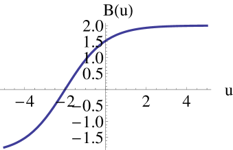
Figure 1: Branch 1 solutions for $B(u)$ and $K(u)$, with $C_{1},\ell=1,C_{2}=2$.

In Figure 1, we illustrate a typical form of the solutions from branch 1. Since $B(u)$ and $K(u)$, as well as their derivatives, are bounded functions, the field strengths (4.2) and (4.3) approach asymptotically to a Riemannian AdS spacetime. This motivates us to examine the corresponding asymptotic structure in more details.

5 Asymptotic symmetry

In this section, we use the canonical approach to analyze the asymptotic symmetry associated to the Vaidya–OTT solution with torsion in branch 1.

5.1 AdS asymptotic conditions

Transition from the OTT to the Vaidya–OTT triad is realized not only by making $B$ a function of $u$, but also by going over to a new triad basis, as can be seen by comparing Eqs. (2.2) and (3.3). The new basis allowed us to introduce the RC geometry by the simple rules formulated in subsection 4.1. Then, requiring the invariance under the AdS group $SO(2,2)$, see [20], one arrives at the following set of the Vaidya–OTT asymptotic states:

$$b^{i}{{}_{\mu}}=\bar{b}^{i}{{}_{\mu}}+B^{i}{{}_{\mu}},\qquad\bar{b}^{i}{{}_{\mu}}=\left(\begin{array}[]{lll}1&0&0\\[1.0pt] \displaystyle\frac{r^{2}}{2\ell^{2}}&1&0\\[7.0pt] 0&0&r\end{array}\right),\qquad B^{i}{{}_{\mu}}:=\left(\begin{array}[]{lll}{\cal O}_{1}&{\cal O}_{3}&{\cal O}_{1}\\ {\cal O}_{-1}&{\cal O}_{1}&{\cal O}_{-1}\\ {\cal O}_{0}&{\cal O}_{2}&{\cal O}_{0}\end{array}\right),$$ (5.1a)

and

$$\omega^{i}{{}_{\mu}}=\bar{\omega}^{i}{{}_{\mu}}+\Omega^{i}{{}_{\mu}},\qquad{\bar{\omega}}^{i}{{}_{\mu}}=-\left(\begin{array}[]{lll}0&0&1\\ 0&0&\displaystyle\frac{r^{2}}{2\ell^{2}}\\ \displaystyle\frac{r}{\ell^{2}}&0&0\end{array}\right),\qquad\Omega^{i}{{}_{\mu}}:=\left(\begin{array}[]{lll}{\cal O}_{1}&{\cal O}_{3}&{\cal O}_{1}\\ {\cal O}_{-1}&{\cal O}_{1}&{\cal O}_{-1}\\ {\cal O}_{0}&{\cal O}_{2}&{\cal O}_{0}\end{array}\right),$$ (5.1b)

where $\omega^{i}$ is the Lie dual of $\omega^{ij}$, and $\bar{b}^{i}{{}_{\mu}}$ and ${\bar{\omega}}^{i}{{}_{\mu}}$ refer to the background configuration with $\mu,B=0$, representing the massless BTZ black hole. These states are invariant under the set of restricted local Poincaré transformations, defined by the parameters

$$\xi^{u}=\ell U+{\cal O}_{2}\,,\qquad\xi^{r}=-r\ell\partial_{u}U+{\cal O}_{0}\,,$$

$$\xi^{\varphi}=\Phi-\frac{\ell}{r}\partial_{\varphi}U+{\cal O}_{2}\,,$$ (5.2a)

$$\theta^{+}=-\frac{\ell}{r}\partial_{\varphi}U+{\cal O}_{2}\,,\qquad\theta^{-}=\frac{r}{2\ell}\partial_{\varphi}U+{\cal O}_{0}\,,$$

$$\theta^{2}=\ell\partial_{u}U+{\cal O}_{1}\,.$$ (5.2b)

Here, the functions $U=U(u,\varphi)$ and $\Phi=\Phi(u,\varphi)$ are such that the combinations $U^{\pm}=U\pm\Phi$ satisfy the conditions $\partial_{\pm}U^{\mp}=0$, where $x^{\pm}=u/\ell\pm\varphi$. Since $u=t+{\cal O}_{1}$ for large $r$, these conditions define the asymptotic conformal group in 2D.

In spite of certain technical differences between the asymptotic requirements (5.1) and (B.1), the corresponding commutator algebras have the same form. Using the composition law of the restricted Poincaré parameters to leading order, the commutator algebra associated to (5.1) is found to have the form of two independent Virasoro algebras,

$$i[\ell^{\pm}_{m},\ell^{\pm}_{n}]=(m-n)\ell^{\pm}_{m+n}\,,$$ (5.3)

where $\ell^{\pm}_{n}=\delta_{0}(U^{\pm}=e^{\pm inx^{+}})$. The respective central charges $c^{\pm}$ will be determined by the canonical methods.

To complete the analysis of the asymptotic conditions, we presented in Appendix C an additional set of asymptotic requirements, motivated by the form of torsion in (4.2).

5.2 Canonical generators

In order to examine the canonical structure of the quadratic PGT, we use the first-order formulation [21], as it leads to a particularly simple construction of the canonical generator, the form of which can be found in Eq. (5.7) of Ref. [7]. In this formulation, one introduces two new variables, $\tau_{i}$ and $\rho_{mn}$, such that their on-shell values are $\tau_{i}=H_{i}$ and $\rho_{mn}=H_{mn}$. Since the canonical generator $G$ acts on basic dynamical variables via the Poisson bracket operation, it is required to be a differentiable phase-space functional. For a given set of asymptotic conditions, this property is ensured by adding a suitable surface $\Gamma$ term to $G$, such that ${\tilde{G}}=G+\Gamma$ is both differentiable and finite phase-space functional [22, 23]. To examine the differentiability of $G$, we start from the form of its variation:

$$\delta G=-\int_{\Sigma}d^{2}x(\delta G_{1}+\delta G_{2})\,,$$

$$\delta G_{1}=\varepsilon^{t\alpha\beta}\xi^{\mu}\left(b^{i}{{}_{\mu}}\partial_{\alpha}\delta\tau_{i\beta}+\omega^{i}{{}_{\mu}}\partial_{\alpha}\delta\rho_{i\beta}+\tau^{i}{{}_{\mu}}\partial_{\alpha}\delta b_{i\beta}+\rho^{i}{{}_{\mu}}\partial_{\alpha}\delta\omega_{i}{{}_{\beta}}\right)+R\,,$$

$$\delta G_{2}=\varepsilon^{t\alpha\beta}\theta^{i}\partial_{\alpha}\delta\rho_{i\beta}+R\,.$$ (5.4)

Here, the coherently oriented volume 2-form on the spatial section $\Sigma$ of spacetime is normalized to $d^{2}x=drd\varphi$, the variation is performed in the set of asymptotic states, $R$ stands for regular terms, and $\rho^{i}$ is the Lie dual of $\rho_{mn}=H_{mn}$, the on-shell value of which reads

$$H_{ij}=-2a_{0}\varepsilon_{ijk}b^{k}-4a_{0}\ell^{2}\varepsilon_{ijk}\hat{L}^{k}\,,$$ (5.5)

and $\hat{L}^{k}$ is the “symmetrized” Schouten 1-form, $\hat{L}_{k}=L_{(km)}b^{m}$, see (2.5).

In what follows, we restrict our considerations by two specific assumptions that characterize both the OTT black hole and the Vaidya–OTT solution with torsion:

(1) The torsion squared-terms in $L_{G}$ effectively vanish, that is $\tau_{i}=0$;

(2) ${}^{(5)}R^{ij}=0$.
The asymptotic conditions (5.1) imply $\delta G_{2}=R$, so that the surface term in the improved generator ${\tilde{G}}=G+\Gamma$ is determined by the variational equations

$$\delta\Gamma=\int_{0}^{2\pi}d\varphi(\xi^{t}\delta{\cal E}+\xi^{\varphi}\delta{\cal M})\,,$$ (5.6a)

$$\delta{\cal E}:=\frac{1}{2}\left(\omega^{ij}{{}_{t}}\delta H_{ij\varphi}+\delta\omega_{ij\varphi}H^{ij}{{}_{t}}\right)\,,$$ (5.6b)

$$\delta{\cal M}:=\frac{1}{2}\left(\omega^{ij}{{}_{\varphi}}\delta H_{ij\varphi}+\delta\omega_{ij\varphi}H^{ij}{{}_{\varphi}}\right)\,,$$ (5.6c)

where we used $u=t+{\cal O}_{1}$, and the boundary $\partial\Sigma$ is parametrized by the coordinate $\varphi$.

Finding a solution for ${\cal E}$ from the variational equation (5.6b) demands rather involved considerations, based on the asymptotic conditions (5.1) and (C.1). As shown in Appendix C, the surface term for time translations can be written in the form

$$\Gamma[\xi^{t}] = \int_{0}^{2\pi}d\varphi\,\xi^{t}{\cal E}\,,$$ (5.7a)

$${\cal E} = \frac{1}{2}\bigl{(}\omega^{ij}{{}_{t}}\Delta H_{ij\varphi}+\Delta\omega^{ij}{{}_{\varphi}}\bar{H}_{ijt}\bigr{)}-\frac{1}{4}\bigl{(}\Delta\omega^{ij}{{}_{t}}\Delta H_{ij\varphi}-\Delta\omega^{ij}{{}_{\varphi}}\Delta H_{ijt}\bigr{)}\,,$$ (5.7b)

where $$\Delta X:=X-\bar{X} X \bar{X}$$ is the difference between any form and its boundary value . On the other hand, equation (5.6c) leads to a simple surface term for spatial rotations:

$$\Gamma[\xi^{\varphi}]=\int_{0}^{2\pi}d\varphi\,\xi^{\varphi}{\cal M}\,,\qquad{\cal M}=\frac{1}{2}\omega^{ij}{{}_{\varphi}}H_{ij\varphi}\,.$$ (5.7c)

Both $\Gamma[\xi^{t}]$ and $\Gamma[\xi^{\varphi}]$ are finite phase-space functionals (see Appendix C).

The boundary terms for $\xi^{t}=1$ and $\xi^{\varphi}=1$,

$$E=\int_{0}^{2\pi}d\varphi\,{\cal E}\,,\qquad M=\int_{0}^{2\pi}d\varphi\,{\cal M}\,,$$ (5.8)

represent the energy and angular momentum of the system, respectively. Calculated on the Vaidya–OTT configuration, these expressions take the values

$$E=\frac{1}{4G}\left(\mu+\frac{1}{4}B^{2}\ell^{2}-2K\right)\,,\qquad M=0\,.$$ (5.9)

The form of $E$ confirms the result (4.7) obtained from the Lagrangian field equations. In the canonical formalism, the conservation laws for $E$ and $M$ follow from the Poisson bracket algebra of the asymptotic symmetry [11].

The expression for energy defined by equation (5.7b) consists of two pieces. As shown in Ref. [15], the first piece is sufficient to correctly describe the energy content of a number of solutions in 3D gravity with/without torsion and topologically massive gravity. However, when applied to the (Vaidya–)OTT solution, this piece is not sufficient; in particular, it produces the incorrect coefficient $1/2$ for the $B^{2}$ term in (5.9). The second piece in (5.7b) is closely related to the presence of the $Br$ term in the OTT metric. Thus, our result (5.7b) represents a generalization of the energy formula used in [15] to the (Vaidya–)OTT case.

5.3 Canonical algebra of asymptotic symmetries

The asymptotic symmetry is described by the Poisson bracket algebra of the improved generators. Rather then performing a direct calculation, the form of this algebra can be found by a more instructive method. To show how it works, we introduce the notation ${\tilde{G}}^{\prime}={\tilde{G}}[U^{\prime},\Phi^{\prime}]$, and similarly for ${\tilde{G}}^{\prime\prime}$ and ${\tilde{G}}^{\prime\prime\prime}$. Then, according to the main theorem of Ref. [23], one can conclude that the Poisson bracket algebra has the form

$$\{{\tilde{G}}^{\prime\prime},{\tilde{G}}^{\prime}\}={\tilde{G}}^{\prime\prime\prime}+C^{\prime\prime\prime}\,,$$ (5.10)

where the parameters of ${\tilde{G}}^{\prime\prime\prime}$ are defined by the composition law of the asymptotic Poincaré transformations, and $C^{\prime\prime\prime}$ is the central charge term. In order to calculate $C^{\prime\prime\prime}$, one should note that the algebra (5.10) implies $\delta_{0}^{\prime}\Gamma^{\prime\prime}\approx\Gamma^{\prime\prime\prime}+C^{\prime\prime\prime}$, where $\delta_{0}^{\prime}\Gamma^{\prime\prime}$ is determined by the relations (5.6), and $C^{\prime\prime\prime}$ is identified as the field independent piece on the right-hand side. Then, going over to the Fourier modes $L_{n}^{\pm}$ of ${\tilde{G}}$, the algebra (5.10) takes the form of two independent Virasoro algebras,

$$i\{L^{\pm}_{m},L^{\pm}_{n}\}=(m-n)L^{\pm}_{n+m}+\frac{c^{\pm}}{12}n^{3}\delta_{m,-n}\,,$$ (5.11)

where the classical central charges are equal to each other, $c^{\pm}=c$, with

$$c=\frac{3\ell}{G}\,.$$ (5.12)

Thus, the value of $c$ is found to be twice the GR value $c_{0}=3\ell/2G$.

6 Concluding remarks

In this paper, we constructed a Vaidya-like extension of the OTT black hole as an exact solution of the quadratic PGT in vacuum. The construction is realized in two steps.

First, we showed that the OTT black hole is a Riemannian vacuum solution of PGT, provided the coupling constants satisfy certain requirements. The black hole energy is calculated from the canonical generator for time translations, the surface term of which is a suitable generalization of the more standard expression that can be found in Ref. [14], see also Ref. [15]. The canonical energy $E$ is compatible with the first law of black hole thermodynamics, in agreement with the equality of $E$ to the shifted OTT energy [18].

Then, following Maeda [12], we introduced a Vaidya-like extension of the OTT black hole; however, this extension is not a Riemannian solution of PGT in vacuum. To overcome this difficulty, we introduced a suitable ansatz for the connection possessing a nontrivial torsion content, making thereby the resulting Vaidya–OTT geometry an exact vacuum solution of PGT. As far as the asymptotic structure of the Vaidya–OTT solution is concerned, one should note that: (a) the surface term of the canonical generator for time translations has the same structure as in the OTT case, (b) the canonical energy differs from the OTT black hole energy by a contribution stemming from the torsion, and (c) central charges of the asymptotic algebra are the same as in the OTT black hole case.

Since the OTT solution is known to exists also for positive or vanishing $1/\ell^{2}$ [10], most of the present results could be straightforwardly extended to these sectors.

Appendix A PGT field equations

In this Appendix, we give a brief account of the PGT field equations, based on Ref. [7]. The parity-invariant gravitational Lagrangian $L_{G}=L_{G}(b^{i},T^{j},R^{mn})$ (3-form) is at most quadratic in the torsion $T^{i}$ and the curvature $R^{ij}$:

$$L_{G} = -{{}^{\star}}(a_{0}R+2{\mit\Lambda}_{0})+T^{i}{{}^{\star}}(a_{1}{}^{(1)}T_{i}+a_{2}{}^{(2)}T_{i}+a_{3}{}^{(3)}T_{i})$$ (A.1)

$$+\frac{1}{2}R^{ij}\left(b_{4}{}^{(4)}R_{ij}+b_{5}{}^{(5)}R_{ij}+b_{6}{}^{(6)}R_{ij}\right)\,,$$

where ${}^{(n)}T^{i}$ and ${}^{(n)}R^{ij}$ are irreducible components of the respective field strengths, and $a_{0}$ is normalized by $a_{0}=/16\pi G$. By varying $L_{G}$ with respect to $b^{i}$ and $\omega^{ij}$, one obtains the vacuum field equations that can be written in a compact form as

$$\rm(1ST)\quad \nabla H_{i}+E_{i}=0\,,$$

$$\rm(2ND)\quad \nabla H_{ij}+E_{ij}=0\,.$$ (A.2)

Here, $H_{i}:=\partial L_{G}/\partial T^{i}$ and $H_{ij}:=\partial L_{G}/\partial R^{ij}$ are the covariant momenta:

$$H_{i}=2{{}^{\star}}(a_{1}{}^{(1)}T_{i}+a_{2}{}^{(2)}T_{i}+a_{3}{}^{(3)}T_{i})\,,$$

$$H_{ij}=-2a_{0}\varepsilon_{ijm}b^{m}+H^{\prime}_{ij}\,,$$

$$H^{\prime}_{ij}:=2\,{{}^{\star}}\left(b_{4}{}^{(4)}R_{ij}+b_{5}{}^{(5)}R_{ij}+b_{6}{}^{(6)}R_{ij}\right)\,,$$ (A.3)

and $E_{i}:=\partial L_{G}/\partial b^{i}$ and $E_{ij}=\partial L_{G}/\partial\omega^{ij}$ are the energy-momentum and spin currents:

$$E_{i}=h_{i}\hbox{\vrule height=0.0pt,width=4.0pt,depth=0.3pt\vrule height=7.0pt,width=0.3pt,depth=0.3pt\vrule height=0.0pt,width=2.0pt,depth=0.0pt}\hskip 0.8ptL_{G}-(h_{i}\hbox{\vrule height=0.0pt,width=4.0pt,depth=0.3pt\vrule height=7.0pt,width=0.3pt,depth=0.3pt\vrule height=0.0pt,width=2.0pt,depth=0.0pt}\hskip 0.8ptT^{m})H_{m}-\frac{1}{2}(h_{i}\hbox{\vrule height=0.0pt,width=4.0pt,depth=0.3pt\vrule height=7.0pt,width=0.3pt,depth=0.3pt\vrule height=0.0pt,width=2.0pt,depth=0.0pt}\hskip 0.8ptR^{mn})H_{mn}\,,$$

$$E_{ij}=-(b_{i}H_{j}-b_{j}H_{i})\,.$$ (A.4)

In the Riemannian sector ($T^{i}=0$) with ${}^{(5)}R_{ij}=0$, $H_{i}$ and $E_{ij}$ vanish, and the simplified field equations take the form displayed in (2.7), with

$$H_{ij}=-2a_{0}\varepsilon_{ijm}b^{m}+\frac{b_{6}+2b_{4}}{3}\,R\varepsilon_{ijk}b^{k}-2b_{4}\varepsilon_{ij}{{}^{m}}{(Ric)}_{mk}b^{k}\,,$$

$$E_{i}={\cal L}_{G}{{}^{\star}}b_{i}-R^{mn}{}_{ik}b^{k}H_{mn}\,.$$ (A.5)

Here, we used $L_{G}={\cal L}_{G}\,\hat{\epsilon}$, and $\hat{\epsilon}$ is the volume 3-form.

Appendix B Asymptotic conditions for the OTT black hole

The action of the AdS Killing vectors on the OTT black hole configuration, described in section 2, leads to the associated asymptotic conditions that are relaxed with respect to the Brown-Henneaux ones:

$$b^{i}{{}_{\mu}}=\bar{b}^{i}{{}_{\mu}}+B^{i}{{}_{\mu}}\,,\qquad B^{i}{{}_{\mu}}:=\left(\begin{array}[]{lll}{\cal O}_{0}&{\cal O}_{3}&{\cal O}_{0}\\ {\cal O}_{1}&{\cal O}_{2}&{\cal O}_{1}\\ {\cal O}_{0}&{\cal O}_{3}&{\cal O}_{0}\end{array}\right)\,,$$ (B.1a)

and

$$\omega^{i}{{}_{\mu}}=\bar{\omega}^{i}{{}_{\mu}}+\Omega^{i}{{}_{\mu}}\,,\qquad\Omega^{i}{{}_{\mu}}:=\left(\begin{array}[]{lll}{\cal O}_{0}&{\cal O}_{3}&{\cal O}_{0}\\ {\cal O}_{1}&{\cal O}_{2}&{\cal O}_{1}\\ {\cal O}_{0}&{\cal O}_{3}&{\cal O}_{0}\end{array}\right)\,.$$ (B.1b)

Here, $\omega^{i}$ is the Lie dual of $\omega^{ij}$, and $\bar{b}^{i}{{}_{\mu}}$ and ${\bar{\omega}}^{i}{{}_{\mu}}$ refer to the AdS background (with $B=\mu=0$). These conditions are invariant under the asymptotic Poincaré transformations, defined by the set of restricted local parameters $(\xi^{\mu},\theta^{i})$ that can be found in Ref. [20]. The conditions (B.1) are a PGT generalization of those discussed in [10].

Following the procedure described in section 5, one can find the conserved charges of the OTT black hole, the energy $E$ and the angular momentum $M$. Moreover, the canonical algebra of the asymptotic symmetry is represented by two independent Virasoro algebras with equal central charges $c^{\mp}=c$. The values of $E,M$ and $c$ are given in subsection 2.3.

Appendix C Refined asymptotic conditions

Equation (4.2) implies that the Vaidya–OTT solution has only one nonvanishing component of torsion: $T^{2}{}_{u\varphi}=K$. Clearly, this property is not valid on the whole set of asymptotic states. In order to ensure finiteness of the improved canonical generators, we find it necessary to make further restrictions of the asymptotic conditions (5.1) by demanding the highest order terms in $T^{i}{}_{\mu\nu}$ to vanish:

$$T^{+}{}_{u\varphi}:\quad r\left(\Omega^{+}{{}_{u}}+\frac{1}{\ell^{2}}B^{+}{{}_{\varphi}}\right)+(\Omega^{2}{{}_{\varphi}}+B^{2}{{}_{u}})={\cal O}_{1}\,,$$

$$T^{+}{}_{ur}:\quad\frac{r}{\ell^{2}}B^{+}{{}_{r}}+\Omega^{2}{{}_{r}}+\frac{1}{r}B^{+}{{}_{u}}={\cal O}_{3}\,,$$

$$T^{+}{}_{r\varphi}:\quad r\Omega^{+}{{}_{r}}+B^{2}{{}_{r}}+\frac{1}{r}B^{+}{{}_{\varphi}}={\cal O}_{3}\,,$$ (C.1a)

$$T^{-}{}_{u\varphi}:\quad r\left(\Omega^{-}{{}_{u}}+\frac{1}{\ell^{2}}B^{-}{{}_{\varphi}}\right)+\frac{r^{2}}{2\ell^{2}}(\Omega^{2}{{}_{\varphi}}+B^{2}{{}_{u}})={\cal O}_{0}\,,$$

$$T^{-}{}_{ur}:\quad\frac{r}{\ell^{2}}B^{-}{{}_{r}}+\frac{r^{2}}{2\ell^{2}}\Omega^{2}{{}_{r}}-\Omega^{2}{{}_{u}}-\frac{1}{r}B^{-}{{}_{u}}={\cal O}_{1}\,,$$

$$T^{-}{}_{r\varphi}:\quad\Omega^{2}{{}_{\varphi}}+\frac{r^{2}}{2\ell^{2}}B^{2}{{}_{r}}+r\Omega^{-}{{}_{r}}+\frac{1}{r}B^{-}{{}_{\varphi}}={\cal O}_{1}\,,$$ (C.1b)

$$T^{2}{}_{u\varphi}:\quad\frac{r^{2}}{2\ell^{2}}(\Omega^{+}{{}_{\varphi}}+B^{+}{{}_{u}})-(B^{-}{{}_{u}}+\Omega^{-}{{}_{\varphi}})={\cal O}_{0}\,,$$

$$T^{2}{}_{ur}:\quad\frac{r^{2}}{2\ell^{2}}\Omega^{+}{{}_{r}}-(\Omega^{-}{{}_{r}}+\Omega^{+}{{}_{u}})={\cal O}_{2}\,,$$

$$T^{2}{}_{r\varphi}:\quad\frac{r^{2}}{2\ell^{2}}B^{+}{{}_{r}}+\Omega^{+}{{}_{\varphi}}-B^{-}{{}_{r}}={\cal O}_{2}\,.$$ (C.1c)

Now, we use the asymptotic conditions (5.1) and (C.1) to derive the surface terms (5.7) and prove their finiteness. First, we show that ${\cal E}$ satisfies the variational equation (5.6b):

$$\delta{\cal E} = \frac{1}{2}\left(\omega^{ij}{{}_{t}}\delta H_{ij\varphi}+\delta\omega_{ij\varphi}H^{ij}{{}_{t}}\right)$$ (C.2)

$$+\frac{1}{4}\left(\delta\omega^{ij}{}_{t}\Delta H_{ij\varphi}-\Delta\omega^{ij}{}_{t}\delta H_{ij\varphi}-\delta\omega^{ij}{}_{\varphi}\Delta H_{ijt}+\Delta\omega^{ij}{}_{\varphi}\Delta H_{ijt}\right)$$

$$= \frac{1}{2}\left(\omega^{ij}{{}_{t}}\delta H_{ij\varphi}+\delta\omega_{ij\varphi}H^{ij}{{}_{t}}\right)+{\cal O}_{1}\,,$$

Next, we prove that the surface term for time translations is finite:

$${\cal E} = 2a_{0}\left(\frac{r^{2}}{2\ell^{2}}\Omega^{+}{{}_{\varphi}}+\Omega^{-}{{}_{\varphi}}-r\Omega^{2}{{}_{u}}\right)+{\cal O}_{0}$$ (C.3)

$$= -a_{0}\frac{r^{3}}{\ell^{2}}\left(\frac{1}{r}B^{+}{{}_{u}}+\frac{r}{\ell^{2}}B^{+}{{}_{r}}+\Omega^{2}{{}_{r}}\right)+{\cal O}_{0}={\cal O}_{0}\,.$$

Finally, we derive the finiteness of the surface term for spatial rotations:

$${\cal M} = -a_{0}\varepsilon^{imn}\omega_{mn\varphi}\Bigl{(}b_{i\varphi}+2\ell^{2}L_{(ij)}b^{j}{{}_{\varphi}}\Bigr{)}$$ (C.4)

$$= 2a_{0}\left(rB^{2}{{}_{u}}-B^{-}{{}_{\varphi}}-\frac{1}{2}\frac{r^{2}}{\ell^{2}}B^{+}{{}_{\varphi}}\right)-4a_{0}\ell^{2}\left(r{(Ric)}_{(+2)}+\frac{r^{2}}{2\ell^{2}}{(Ric)}_{(-2)}\right)+{\cal O}_{0}$$

$$= {\cal O}_{0}\,.$$

References

- [1] T. W. B. Kibble, Lorentz invariance and the gravitational field, J. Math. Phys. 2 (1961) 212–221; D. W. Sciama, On the analogy between charge and spin in general relativity, in: Recent Developments in General Relativity, Festschrift for Infeld (Pergamon Press, Oxford; PWN, Warsaw, 1962) pp. 415–439.
- [2] M. Blagojević, Gravitation and Gauge Symmetries (Institute of Physics, Bristol, 2002); T. Ortín, Gravity and Strings (Cambridge University Press, Cambridge, 2004).
- [3] Yu. N. Obukhov, Poincaré gauge gravity: Selected topics, Int. J. Geom. Meth. Mod. Phys. 3 (2006) 95–138.
- [4] M. Blagojević and F. W. Hehl (eds.), Gauge Theories of Gravitation, A Reader with Commentaries (Imperial College Press, London, 2013).
- [5] E. W. Mielke and P. Baekler, Topological gauge model of gravity with torsion, Phys. Lett. A 156 (1991) 399–403.
- [6] J. A. Helayël-Neto, C. A. Hernaski, B. Pereira-Dias, A. A. Vargas-Paredes, and V. J. Vasquez-Otoya, Chern-Simons gravity with (curvature)2- and (torsion)2-terms and a basis of degree-of-freedom projection operators, Phys. Rev. D 82 (2010) 064014.
- [7] M. Blagojević and B. Cvetković, 3D gravity with propagating torsion: the AdS sector, Phys. Rev. D85 (2012) 104003 [10 pages].
- [8] M. Blagojević and B. Cvetković, Gravitational waves with torsion in 3D, Phys. Rev. D90 (2014) 044006 [9 pages].
- [9] M. Blagojević and B. Cvetković, Siklos waves with torsion in 3D, JHEP 1411 (2014) 141 [16 pages].
- [10] J. Oliva, D. Tempo, and R. Troncoso, Three-dimensional black holes, gravitational solitons, kinks and wormholes for BHT massive gravity, JHEP 07 (2009) 011 [25 pages].
- [11] J. Oliva, D. Tempo, and R. Troncoso, Static spherically symmetric solutions for conformal gravity in three dimensions, Int. J. Mod. Phys. A 24 (2009) 1588–1592.
- [12] H. Maeda, Black-hole dynamics in BHT massive gravity, JHEP 1102 (2011) 039 [7 pages].
- [13] E. A. Bergshoeff, O. Hohm and P. K. Townsend, Massive gravity in three dimensions, Phys. Rev. Lett. 102 (2009) 201301.
- [14] J. M. Nester, C.-M. Chen and Y.-H. Wu, Gravitational energy-momentum in MAG, preprint arXiv:gr-qc/0011101v1.
- [15] M. Blagojević and B. Cvetković, Conserved charges in 3D gravity, Phys. Rev. D81 (2010) 124024 [7 pages].
- [16] M. Blagojević and B. Cvetković, Extra gauge symmetries in BHT gravity, JHEP 1103 (2011) 139 [13 pages].
- [17] O. Hohm, A. Routh, P. K. Townsend, and B. Zhang, On the Hamiltonian form of 3D massive gravity, Phys. Rev. D86 (2012) 084035.
- [18] G. Giribet, J. Oliva, D. Tempo, and R. Troncoso, Microscopic entropy of the three-dimensional rotating black hole of BHT massive gravity Phys. Rev. D80 (2009) 124046.
- [19] T. Padmanabhan, Gravitation, Foundations and Frontiers (Cambridge University Press, Cambridge, 2010), chapter 7.
- [20] M. Blagojević and B. Cvetković, Canonical structure of 3D gravity with torsion, in: Trends in General Relativity and Quantum Cosmology, edited by C. Benton, vol. 2 (Nova Science Publishers, New York, 2006) pp. 103–123.
- [21] J. M. Nester, A covariant Hamiltonian for gravity theories, Mod. Phys. Lett. A6 (1991) 2655–2661.
- [22] T. Regge and C. Teitelboim, Role of surface integrals in the Hamiltonian formulation of general relativity, Ann. Phys. (N.Y) 88 (1974) 286–318.
- [23] J. D. Brown and M. Hennaux, On the Poisson brackets of differentiable generators in classical field theory, J. Math. Phys. 27 (1986) 489–491.