Approximating the Minimum Breakpoint Linearization Problem for Genetic Maps without Gene Strandedness

Abstract

The study of genetic map linearization leads to a combinatorial hard problem, called the minimum breakpoint linearization (MBL) problem. It is aimed at finding a linearization of a partial order which attains the minimum breakpoint distance to a reference total order. The approximation algorithms previously developed for the MBL problem are only applicable to genetic maps in which genes or markers are represented as signed integers. However, current genetic mapping techniques generally do not specify gene strandedness so that genes can only be represented as unsigned integers. In this paper, we study the MBL problem in the latter more realistic case. An approximation algorithm is thus developed, which achieves a ratio of $(m^{2}+2m-1)$ and runs in $O(n^{7})$ time, where $m$ is the number of genetic maps used to construct the input partial order and $n$ the total number of distinct genes in these maps.

Index terms — Comparative genomics, partial order, breakpoint distance, feedback vertex set.

1 Introduction

Genetic map linearization is a crucial preliminary step to most comparative genomics studies, because they generally require a total order of genes or markers on a chromosome rather than a partial order that current genetic mapping techniques might only suffice to provide [2, 6, 8, 9]. One of the computational approaches proposed for genetic map linearization is to find a topological sort of the directed acyclic graph (DAG) that represents the input genetic maps while minimizing its breakpoint distance to a reference total order. It hence leads to a combinatorial optimization problem, called the minimum breakpoint linearization (MBL) problem [2], which has attracted great research attention in the past few years [2, 3, 4, 6].

The MBL problem is already shown to be NP-hard [2], and even APX-hard [3]. The first algorithm proposed to solve the MBL problem is an exact dynamic programming algorithm running in exponential time in the worst case [2]. In the same paper, a time-efficient heuristic algorithm is also presented, which, however, has no performance guarantee. The first attempt was made in [4] to develop a polynomial-time approximation algorithm. Unfortunately, the proposed algorithm was latter found invalid [3] because it relies on a flawed statement in [6] on adjacency-order graphs. To fix this flaw, the authors of [3] revised the construction of adjacency-order graphs and proposed three approximation algorithms, two of which are based on the existing approximation algorithms for a general variant of the feedback vertex set problem, and the third was instead developed in the same spirit as was done in [4], achieving a ratio of $(m^{2}+4m-4)$ (only for $m\geq 2$).

As we shall show in Section 2.3, the above approximation algorithms are only applicable to the input genetic maps in which genes or markers are represented as signed integers, where the signs represent the strands of genes/markers. However, we note that the original definition of the MBL problem assumes unsigned integers for genes [2]. In fact, this is a more realistic case. Current genetic mapping techniques such as recombination analysis and physical imaging generally do not specify gene strandedness so that genes can only be represented as unsigned integers [8]. Based on this observation, whether the MBL problem can be approximated still remains a question not yet to be resolved.

In this paper, we study the MBL problem in the more realistic case where no gene strandedness information is available for the input genetic maps. We revised the definition of conflict-cycle in [3], from which an approximation algorithm is hence developed also in the same spirit as done in [3, 4]. It achieves a ratio of $(m^{2}+2m-1)$ (which holds for all $m\geq 1$) and runs in $O(n^{7})$ time, where $m$ is the number of genetic maps used to construct the input partial order and $n$ the total number of distinct genes occurring in these maps.

The rest of the paper is organized as follows. We first introduce some preliminaries and notations in Section 2. In Section 3 we discuss a number of basic facts about the MBL problem, which leads to the formulation of the minimum breakpoint vertex set (MBVS) problem in Section 4. We present an approximation algorithm for the MBL problem via the approximation of the MBVS problem in Section 4, and then conduct performance analyses on both its approximation ratio and running time in Section 5. Finally, some concluding remarks are made in Section 6. For the sake of consistency, we borrowed many notations from [3] and [4] throughout the paper.

2 Preliminaries and notations

2.1 Genetic maps and their combined directed acyclic graph

A genetic map is a totally-ordered sequence of blocks, each of which comprises one or more genes. It defines a partial order on genes, where genes within a block are ordered before all those in its succeeding blocks, but unordered among themselves.

Today it is increasingly common to find multiple genetic maps available for a same genome. Combining these maps often provides a partial order with a higher coverage of gene ordering than an individual genetic map. To represent this partial order, we may construct a directed acyclic graph $\Pi=(\Sigma,D)$, where the vertex set $\Sigma=\{1,\dots,n\}$ is made of all the contributing genes and the arc set $D$ made of all the ordered pairs of genes appearing in consecutive blocks of the same genetic map [7, 8]. Two properties can be deduced [3] from these genetic maps and their combined directed acyclic graph: (i) if there is an arc between two genes $i$ and $j$ in $\Pi$, then $i$ and $j$ appear in consecutive blocks of some genetic map, and (ii) if $i$ and $j$ appear in different blocks of the same genetic map, then there exists in $\Pi$ a nonempty directed path either from $i$ to $j$ or from $j$ to $i$. See Figure 1 for a simple example of $\Pi$ constructed from two genetic maps.

We say gene $i$ is ordered before (resp. after) gene $j$ by $\Pi$ if there exists in $\Pi$ a nonempty directed path from $i$ to $j$ (resp. $j$ to $i$). We use $i\prec_{\Pi}j$ to denote the ordering relation that gene $i$ is ordered before gene $j$ by $\Pi$. Unlike in [5], we assume in this paper that combining multiple genetic maps would never create order conflicts, i.e., we could not have both $i\prec_{\Pi}j$ and $j\prec_{\Pi}i$ simultaneously.

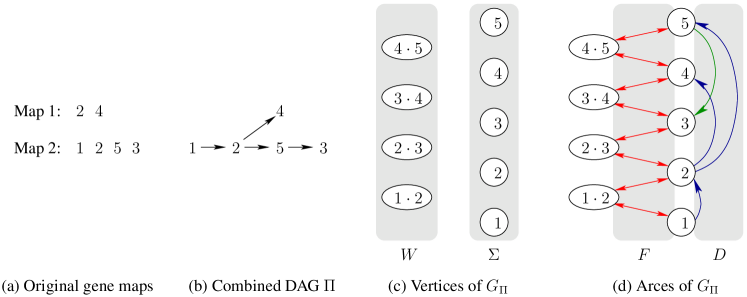
Figure 1: The construction of an adjacency-order graph as proposed in [3]. The symmetric arcs in $F$ are represented as double arrows.

2.2 The minimum breakpoint linearization problem

Let $\Pi=(\Sigma,D)$ be a directed acyclic graph representing a partial order generated with $m$ genetic maps of a same genome. A linearization of $\Pi$ is a total order of genes $\pi=\pi(1)\cdot\pi(2)\cdots\pi(n)$, i.e., a permutation on $\{1,2,\dots,n\}$, such that, for all genes $i,j$, if $i\prec_{\Pi}j$ then $i\prec_{\pi}j$. In this case, $\pi$ is said to be compatible with $\Pi$. Let $\Gamma$ denote another genome with the same set of genes in a total order. Without loss of generality, we assume that $\Gamma$ is the identity permutation $1\ 2\ \cdots\ n$. A pair of genes that are adjacent in $\pi$ but not in $\Gamma$ is called a breakpoint of $\pi$ with respect to $\Gamma$, and the total number of breakpoints is thus defined as the breakpoint distance between $\pi$ and $\Gamma$ [1].

Given a partial order $\Pi$ and a total order $\Gamma$ as described above, the minimum breakpoint linearization (MBL) problem is defined as to find a linearization $\pi$ of $\Pi$ such that the breakpoint distance between $\pi$ and $\Gamma$ is minimized [2]. This minimum breakpoint distance is further referred to as the breakpoint distance between $\Pi$ and $\Gamma$, and denoted by $d_{b}(\Pi,\Gamma)$.

2.3 Adjacency-Order Graph

In this study we adopt the definition of adjacency-order graph introduced in [3]. To construct an adjacency-order graph for a partial order $\Pi=(\Sigma,D)$, we first create a set $W$ of vertices representing the adjacencies of the identity permutation $\Gamma$ by $W=\{i\cdot(i+1)|1\leq i<n\}$, and let $V=\Sigma\cup W$ (see Figure 1c). We will not distinguish the vertices of $\Sigma$ and their corresponding integers, which is always be clear from the context. Then, we construct a set of arcs $F$ as

$$F\ =\ \{i\cdot(i+1)\to i,\ i\cdot(i+1)\to i+1,\ i\to i\cdot(i+1),\ i+1\to i\cdot(i+1)\ |\ 1\leq i<n\},$$

where the arrow $\to$ is used to denote an arc. Note that every arc in $F$ has one end in $W$ and the other end in $\Sigma$. Let $E=D\cup F$ (see Figure 1d). Finally, we define the adjacency-order graph $G_{\Pi}$ of $\Pi$ by $G_{\Pi}=(V,E)$.

Note that in $G_{\Pi}$, the arcs of $D$ may go either top-down or bottom-up. Let $X[G_{\Pi}]$ (or only $X$, if there is no ambiguity) be the set of arcs in $D$ that go top-down, and $Y[G_{\Pi}]$ (or only $Y$) the set of arcs in $D$ that go bottom-up. Formally, we may write $X[G_{\Pi}]=\{i\to j\in D\ |\ i>j\}$ and $Y[G_{\Pi}]=\{i\to j\in D\ |\ i<j\}$. It is easy to see that $D=X\cup Y$ and $X\cap Y=\emptyset$.

In [3], a conflict-cycle refers to a cycle that uses an arc from $X$. By this definition, a conflict-cycle may not necessarily use any arc from $Y$ and all its adjacencies might still co-exist in some linearization of $\Pi$, as we can see from the adjacency-order graph $G_{\Pi}$ shown in Figure 1d. This adjacency-order graph contains a conflict-cycle $3\to 3\cdot 4\to 4\to 4\cdot 5\to 5\to 3$ (as defined in [3]), for which both adjacencies $3\cdot 4$ and $4\cdot 5$ may occur in the linearization $1\ 2\ 5\ 4\ 3$ of $\Pi$. Based on these observations, in this study we use a different definition of conflict-cycles as follows.

Definition 2.1

A cycle in $G_{\Pi}$ is called a conflict-cycle if it contains at least one arc from $X$ and at least one arc from $Y$.

This new definition has wide implications for the future approximation of the MBL problem, as we shall see latter. A quick look indicates that the example cycle mentioned above is no longer a conflict-cycle. In Theorem 3.10, we shall prove that the adjacencies involved in a conflict-cycle could not co-exist in any linearization of $\Pi$. Consequently, we need to remove at least one adjacency from each of those cycles in order to obtain a linearization of $\Pi$.

Most of the following notations are already introduced in [3]. An arc between $u$ and $v$ is written $u\to v$, or $u\to_{A}v$ if it belongs to some set $A$. A path $P$ is a (possibly empty) sequence of arcs written $u\xrightarrow{P}{}^{*}v$, or $u\xrightarrow{P}{}_{A}^{*}v$ if $P$ uses arcs only from $A$. A nonempty path $Q$ is written as $u\xrightarrow{Q}{}^{+}v$ with a $+$ sign. A cycle is a nonempty path $u\xrightarrow{\mathcal{C}}{}^{+}v$ with $v=u$. Given a path $P=v_{0}\to v_{1}\to\dots\to v_{l}$ in $G_{\Pi}$, the following notations are used: $l(P)=l$ is the length of $P$, $V(P)=\{v_{h}\ |\ 0\leq h\leq l\}$, $W(P)=V(P)\cap W$, $\Sigma(P)=V(P)\cap\Sigma$, $E(P)=\{v_{h}\to v_{h+1}\ |\ 0\leq h<l\}$, $F(P)=E(P)\cap F$, $D(P)=E(P)\cap D$, $X(P)=E(P)\cap X$, and $Y(P)=E(P)\cap Y$. A cycle $\mathcal{C}$ is said to be simple if all vertices $v_{h}$ are distinct except $v_{0}=v_{h}$, which implies that $l(\mathcal{C})=|V(\mathcal{C})|=|E(\mathcal{C})|$. If a cycle $\mathcal{C}$ is not simple, then it contains a subcycle $\mathcal{C}^{{}^{\prime}}$ such that $V(\mathcal{C}^{{}^{\prime}})\subseteq V(\mathcal{C})$ and $E(\mathcal{C}^{{}^{\prime}})\subseteq E(\mathcal{C})$. In this paper, we further require $\mathcal{C}^{{}^{\prime}}\neq\mathcal{C}$ when $\mathcal{C}^{{}^{\prime}}$ is the subcycle of $\mathcal{C}$.

3 Some basic facts

Given a cycle $\mathcal{C}$ in $G_{\Pi}$, we may partition $W(\mathcal{C})$ into a collection of disjoint subsets $W_{h}(\mathcal{C})$ such that each of them can be written as $\{i\cdot(i+1)\ |\ a_{h}\leq i<b_{h}\}$, for some integers $a_{h}$ and $b_{h}$. We denote such a collection of disjoint subsets with minimum cardinality by $\mathbb{W}(\mathcal{C})=\{W_{1}(\mathcal{C}),W_{2}(\mathcal{C}),\cdots,W_{l}(\mathcal{C})\}$. Note that, for every cycle $\mathcal{C}$ in $G_{\Pi}$, we have $l=|\mathbb{W}(\mathcal{C})|\geq 1$ because $\Pi=(\Sigma,D)$ is a directed acyclic graph.

Lemma 3.1

Let $\mathcal{C}$ be a (not necessarily simple) cycle with $W_{1}(\mathcal{C})=\{i\cdot(i+1)\ |\ a_{1}\leq i<b_{1}\}$ and $W_{2}(\mathcal{C})=\{i\cdot(i+1)\ |\ a_{2}\leq i<b_{2}\}$ being two distinct elements of $\mathbb{W}(\mathcal{C})$. Then, we have $[a_{1},b_{1}]\cap[a_{2},b_{2}]=\emptyset$.

Proof. By contradiction, suppose that $[a_{1},b_{1}]\cap[a_{2},b_{2}]\neq\emptyset$, which implies that $a_{1}\leq b_{2}$ and $a_{2}\leq b_{1}$. Let $a=\min(a_{1},a_{2})$ and $b=\max(b_{1},b_{2})$, and let $W_{1}^{{}^{\prime}}(\mathcal{C})=\{i\cdot(i+1)\ |\ a\leq i<b\}$. For $\forall i\in[a_{1},b_{1}]\cup[a_{2},b_{2}]$, we have $i\in[a,b]$, which implies that $W_{1}(\mathcal{C})\cup W_{2}(\mathcal{C})\subseteq W_{1}^{{}^{\prime}}(\mathcal{C})$. Next we show that, for $\forall i\in[a,b)$, we have either $i\in[a_{1},b_{1})$ or $i\in[a_{2},b_{2})$. If $i\notin[a_{1},b_{1})$, then $i\geq b_{1}$ since $i\geq a_{1}$ and, further, $i\geq a_{2}$ since $a_{2}\leq b_{1}$. On the other hand, we have $i<b_{2}$ because $i<b=\max(b_{1},b_{2})$. It hence follows that $i\in[a_{2},b_{2})$ if $i\notin[a_{1},b_{1})$. No matter in which case, i.e., either $i\in[a_{1},b_{1})$ or $i\in[a_{2},b_{2})$, we can have $W_{1}^{{}^{\prime}}(\mathcal{C})\subseteq W_{1}(\mathcal{C})\cup W_{2}(\mathcal{C})$. Thus, $W_{1}(\mathcal{C})\cup W_{2}(\mathcal{C})=W_{1}^{{}^{\prime}}(\mathcal{C})$. Consequently, we can obtain a smaller-sized partition of $W(\mathcal{C})$ by replacing two sets $W_{1}(\mathcal{C})$ and $W_{2}(\mathcal{C})$ of the current partition $\mathbb{W}(\mathcal{C})$ with one set $W_{1}^{{}^{\prime}}(\mathcal{C})$, which however contradicts the fact that $\mathbb{W}(\mathcal{C})$ attains the minimum cardinality.        

Lemma 3.2

Let $\mathcal{C}$ be a (not necessarily simple) cycle with $W_{1}(\mathcal{C})=\{i\cdot(i+1)\ |\ a\leq i<b\}$ being an element of $\mathbb{W}(\mathcal{C})$. If there exists a vertex $c\in\Sigma(\mathcal{C})$ such that $c\notin[a,b]$, then $\mathcal{C}$ is a conflict-cycle.

Proof. We first assume that $c<a$. Define $a^{+}=\{i|i\geq a\}\cup\{i\cdot(i+1)|i\geq a\}$ and $a^{-}=\{i|i<a\}\cup\{i\cdot(i+1)|i<a\}$. Then, $a^{+}\cup a^{-}$ is a partition of $V$. Note that there exists in $F$ exactly one arc from $a^{+}$ to $a^{-}$ and exactly one arc from $a^{-}$ to $a^{+}$, i.e., $a\to(a-1)_{F}\cdot a$ and $(a-1)_{F}\cdot a\to a$, respectively. Suppose that $\mathcal{C}$ does not contain any arc from $X$. Since $\mathcal{C}$ contains vertices in both $a^{+}$ and $a^{-}$ (resp. $b$ and $c$), it thus contains an arc $u\to v$ with $u\in a^{+}$ and $v\in a^{-}$. We must have $u\to v\in F$; otherwise, $u\to v\in D$ implies that $u\to v\in X$ since $u>v$. Consequently, we can only have $u=a$ and $v=(a-1)\cdot a$ by the definitions of $a^{+}$ and $a^{-}$. So, $\mathcal{C}$ uses the vertex $(a-1)\cdot a$. However, $W_{1}(\mathcal{C})=\{i\cdot(i+1)\ |\ a\leq i<b\}$ is an element of $\mathbb{W}(\mathcal{C})$, which, by definition, implies that $\mathcal{C}$ does not use the vertex $(a-1)\cdot a$; a contradiction. Therefore, $\mathcal{C}$ must contain an arc from $X$. Now we suppose that $\mathcal{C}$ does not contain any arc from $Y$. Once again, since $\mathcal{C}$ contains vertices in both $a^{+}$ and $a^{-}$, it thus contains an arc $u\to v$ with $u\in a^{-}$ and $v\in a^{+}$. We must have $u\to v\in F$; otherwise, $u\to v\in D$ implies that $u\to v\in Y$ since $u<v$. Consequently, we can only have $u=(a-1)\cdot a$ and $v=a$. So, $\mathcal{C}$ also necessarily uses the vertex $(a-1)\cdot a$. As we show above, it would lead to a contradiction. Therefore, $\mathcal{C}$ must contain an arc from $Y$ too. It turns out that $\mathcal{C}$ is a conflict-cycle.

In case of $c>b$, we may define $b^{+}=\{i|i>b\}\cup\{i\cdot(i+1)|i\geq b\}$ and $b^{-}=\{i|i\leq b\}\cup\{i\cdot(i+1)|i<b\}$. Then, by using the same arguments as above, we can also show that $\mathcal{C}$ is a conflict-cycle.        

Lemma 3.3

Let $\pi$ be a total order that contains every adjacency in the set $\{i\cdot(i+1)\ |\ a\leq i<b\}$. Then, either the sequence $a\ (a+1)\ (a+2)\ \cdots\ b$ or $b\ (b-1)\ (b-2)\ \cdots\ a$ is an interval of $\pi$.

Proof. Recall that an adjacency $i\cdot(i+1)$ implies the occurrence of an interval either $i\ (i+1)$ or $(i+1)\ i$, but not both, in $\pi$. We first consider the adjacency $a\cdot(a+1)$, for which the interval either $a\ (a+1)$ or $(a+1)\ a$ would occur in $\pi$. We distinguish these two cases when the next adjacency $(a+1)\cdot(a+2)$ is considered. In the first case of the interval $a\ (a+1)$, in order to obtain the adjacency $(a+1)\cdot(a+2)$ in $\pi$, the element $(a+2)$ can only appear immediately after the element $(a+1)$, resulting in the interval $a\ (a+1)\ (a+2)$. In the second case of the interval $(a+1)\ a$, in order to obtain the adjacency $(a+1)\cdot(a+2)$ in $\pi$, the element $(a+2)$ can only appear immediately before the element $(a+1)$, resulting in the interval $(a+2)\ (a+1)\ a$. Continue this process with the remaining adjacencies in the increasing order of elements. It would necessarily end up with an interval either $a\ (a+1)\ (a+2)\ \cdots\ b$ or $b\ (b-1)\ (b-2)\ \cdots\ a$ in $\pi$.        

Lemma 3.4

Let $\pi$ be a total order that contains every adjacency in the set $\{i\cdot(i+1)\ |\ a\leq i<b\}$. Assume that there exists in $G_{\Pi}$ an arc $i_{1}\to i_{2}\in D$, where $a\leq i_{1}\leq b$ and $a\leq i_{2}\leq b$. If $i_{1}<i_{2}$ (resp., $i_{1}>i_{2}$), then the sequence $a\ (a+1)\ (a+2)\ \cdots b$ (resp., $b\ (b-1)\ (b-2)\ \cdots a$) is an interval of $\pi$.

Proof. The proof is given only for the case of $i_{1}<i_{2}$. We know from Lemma 3.3 that $\pi$ contains either the interval $a\ (a+1)\ (a+2)\ \cdots\ i_{1}\cdots\ i_{2}\cdots\ b$ or $b\ (b-1)\ (b-2)\ \cdots\ i_{2}\cdots\ i_{1}\cdots\ a$. On the other hand, we have $i_{1}\prec_{\pi}i_{2}$, since there exists an arc $i_{1}\to i_{2}\in D$. Consequently, the interval $b\ (b-1)\ (b-2)\ \cdots\ i_{2}\cdots\ i_{1}\cdots\ a$ could not appear in $\pi$.        

We wish to distinguish two types of conflict-cycles. A conflict-cycle $\mathcal{C}$ is said to be of type I if there exist two vertices $a$ and $b$ in $\Sigma(\mathcal{C})$ such that $V(\mathcal{C})=\{i\cdot(i+1)\ |\ a\leq i<b\}\cup\{i\ |\ a\leq i\leq b\}$; otherwise, it is said to be of type II. For example, in the adjacency-order graph shown in Figure 1, the cycle $1\to 2\to 2\cdot 3\to 3\to 3\cdot 4\to 4\to 4\cdot 5\to 5\to 3\to 2\cdot 3\to 2\to 1\cdot 2\to 1$ is a conflict-cycle of type I, while both $2\to 5\to 3\to 2\cdot 3\to 2$ and $2\to 4\to 4\cdot 5\to 5\to 3\to 2\cdot 3\to 2$ are conflict-cycles of type II. Lemmas 3.5 and 3.6 below follows from the above definitions in a straightforward way.

Lemma 3.5

Let $\mathcal{C}$ is a (not necessarily simple) conflict-cycle of type 1. Then, $|\mathbb{W}(\mathcal{C})|=1$.

Lemma 3.6

Let $\mathcal{C}$ is a (not necessarily simple) cycle with $W_{1}(\mathcal{C})=\{i\cdot(i+1)\ |\ a\leq i<b\}$ being an element of $\mathbb{W}(\mathcal{C})$. Then, $\mathcal{C}$ is a conflict-cycle of type II iff there exists a vertex $c\in\Sigma(\mathcal{C})$ such that $c\notin[a,b]$.

By considering Lemmas 3.1 and 3.2, we can further obtain the following lemma.

Lemma 3.7

Let $\mathcal{C}$ be a (not necessarily simple) cycle with $|\mathbb{W}(\mathcal{C})|\geq 2$. Then, $\mathcal{C}$ is a conflict-cycle of type II.

The first implication of our new definition of conflict-cycle is that a conflict-cycle does not necessarily contain a simple conflict-subcycle.

Lemma 3.8

If $\mathcal{C}$ is a conflict-cycle of type I, then it cannot be a simple cycle.

Proof. By contradiction, suppose that $\mathcal{C}$ is simple. By definition of a type I conflict-cycle, there exist two vertices $a$ and $b$ such that $V(\mathcal{C})=\{i\cdot(i+1)\ |\ a\leq i<b\}\cup\{i\ |\ a\leq i\leq b\}$. Since $\mathcal{C}$ is simple, every vertex in $V(\mathcal{C})$ is adjacent to exactly two distinct vertices in $\mathcal{C}$; therefore, every vertex has indegree and outdegree both exactly one in $\mathcal{C}$. Knowing that every vertex $i\cdot(i+1)\in W$ has only two distinct adjacent vertices in $G_{\Pi}$, i.e., $i$ and $(i+1)$, we can deduce that, for every vertex $i$ such that $a<i<b$, it is adjacent to both $(i-1)\cdot i$ and $i\cdot(i+1)$ by using arcs from $F$. And, the vertex $a$ is adjacent to $a\cdot(a+1)$ and the vertex $b$ is adjacent to $(b-1)\cdot b$, both using arcs also from $F$. Consequently, $\mathcal{C}$ shall contain an arc between $a$ and $b$ so that both vertices have degree two (because any other vertices can no longer be incident to an arc of $D(\mathcal{C})$). Moreover, this arc is the only arc that $\mathcal{C}$ has from $D(\mathcal{C})$, which contradicts the fact that a conflict-cycle shall contain at least two arcs from $D(\mathcal{C})$, i.e., at least one from $X(\mathcal{C})$ and at least one from $Y(\mathcal{C})$.        

Lemma 3.9

If $\mathcal{C}$ is a non-simple conflict-cycle of type II, then it must contain a simple conflict-subcycle of type II.

Proof. Let $\mathbb{W}(\mathcal{C})=\{W_{1}(\mathcal{C}),W_{2}(\mathcal{C}),\cdots,W_{l}(\mathcal{C})\}$. Since $\mathcal{C}$ is not simple, there exists a vertex $u$ used twice in it such that $\mathcal{C}=u\xrightarrow{P}{}^{+}u\xrightarrow{Q}{}^{+}u$. We can further assume that $u\in\Sigma(\mathcal{C})$. If initially we have $u\in W(\mathcal{C})$ such that $u=a\cdot(a+1)$, then $\mathcal{C}$ uses both vertices $a$ and $(a+1)$ at least twice because it uses the vertex $u=a\cdot(a+1)$ twice. So, we may substitute $u$ by $a$ to write $\mathcal{C}=u\xrightarrow{P}{}^{+}u\xrightarrow{Q}{}^{+}u$.

Let $\mathcal{C}_{1}=u\xrightarrow{P}{}^{+}u$ and $\mathcal{C}_{2}=u\xrightarrow{Q}{}^{+}u$. Apparently, $\mathcal{C}_{1}$ and $\mathcal{C}_{2}$ are two subcycles of $\mathcal{C}$, so we write $\mathbb{W}(\mathcal{C}_{1})=\{W_{1}(\mathcal{C}_{1}),W_{2}(\mathcal{C}_{1}),\cdots,W_{l_{1}}(\mathcal{C}_{1})\}$ and $\mathbb{W}(\mathcal{C}_{2})=\{W_{1}(\mathcal{C}_{2}),W_{2}(\mathcal{C}_{2}),\cdots,W_{l_{2}}(\mathcal{C}_{2})\}$, where $l_{1}\geq 1$ and $l_{2}\geq 1$. Note that every element of $\mathbb{W}(\mathcal{C}_{1})$ and of $\mathbb{W}(\mathcal{C}_{2})$ is a subset of an element of $\mathbb{W}(\mathcal{C})$. Below we distinguish two possible cases.

In the first case, we assume that there exist an element of $\mathbb{W}(\mathcal{C}_{1})$ and an element of $\mathbb{W}(\mathcal{C}_{2})$ (say, $W_{1}(\mathcal{C}_{1})=\{i\cdot(i+1)\ |\ a_{11}\leq i<b_{11}\}$ and $W_{1}(\mathcal{C}_{2})=\{i\cdot(i+1)\ |\ a_{21}\leq i<b_{21}\}$, respectively) such that both are the subsets of a same element of $\mathbb{W}(\mathcal{C})$ (say, $W_{1}(\mathcal{C})=\{i\cdot(i+1)\ |\ a_{1}\leq i<b_{1}\}$). It hence implies that $a_{1}\leq a_{11}<b_{11}\leq b_{1}$ and $a_{1}\leq a_{21}<b_{21}\leq b_{1}$. Since $\mathcal{C}$ is a conflict-cycle of type II, by Lemma 3.6, there exists a vertex $c_{1}\in\Sigma(\mathcal{C})$ such that $c_{1}\notin[a_{1},b_{1}]$. Thus, we have both $c_{1}\notin[a_{11},b_{11}]$ and $c_{1}\notin[a_{21},b_{21}]$. Note that the vertex $c_{1}$ appears on the cycle either $\mathcal{C}_{1}$ or $\mathcal{C}_{2}$. If $c_{1}$ appears on $\mathcal{C}_{1}$, then $\mathcal{C}_{1}$ is a conflict-cycle (by Lemma 3.2). Otherwise, $c_{2}$ must appear on $\mathcal{C}_{2}$. By Lemma 3.2 once again, $\mathcal{C}_{2}$ would be a conflict-cycle. Moreover, this conflict-cycle, no matter $\mathcal{C}_{1}$ or $\mathcal{C}_{2}$, is of type II (by Lemma 3.7).

In the second case, we assume that no two elements of $\mathbb{W}(\mathcal{C}_{1})$ and $\mathbb{W}(\mathcal{C}_{2})$ are the subsets of a same element of $\mathbb{W}(\mathcal{C})$. Consider the first elements of $\mathbb{W}(\mathcal{C}_{1})$ and $\mathbb{W}(\mathcal{C}_{2})$, and write them as $W_{1}(\mathcal{C}_{1})=\{i\cdot(i+1)\ |\ a_{11}\leq i<b_{11}\}$ and $W_{1}(\mathcal{C}_{2})=\{i\cdot(i+1)\ |\ a_{21}\leq i<b_{21}\}$, respectively. Note that $W_{1}(\mathcal{C}_{1})$ and $W_{1}(\mathcal{C}_{2})$ are the subsets of two distinct elements (say, $W_{1}(\mathcal{C})=\{i\cdot(i+1)\ |\ a_{1}\leq i<b_{1}\}$ and $W_{2}(\mathcal{C})=\{i\cdot(i+1)\ |\ a_{2}\leq i<b_{2}\}$) of $\mathbb{W}(\mathcal{C})$, respectively). Thus, we have $[a_{11},b_{11}]\subseteq[a_{1},b_{1}]$ and $[a_{21},b_{21}]\subseteq[a_{2},b_{2}]$ and, furthermore, $[a_{11},b_{11}]\cap[a_{21},b_{21}]=\emptyset$ since $[a_{1},b_{1}]\cap[a_{2},b_{2}]=\emptyset$. It then follows that we have either $u\notin[a_{11},b_{11}]$ or $u\notin[a_{21},b_{21}]$. If $u\notin[a_{11},b_{11}]$, $\mathcal{C}_{1}$ would be a conflict-cycle of type II. If $u\notin[a_{21},b_{21}]$, $\mathcal{C}_{2}$ would be a conflict-cycle of type II.

In either case above, we already show that there exists a conflict-subcycle of type II for $\mathcal{C}$. If this conflict-subcycle is not simple, we may apply the above process recursively, which necessarily ends up with a simple conflict-subcycle of type II.        

Although the following theorem appears as a verbatim account of Theorem 4 in [3], they are literally not the same because conflict-cycles are defined in different ways. Consequently, the corresponding proof given in [3] is not sufficient.

Theorem 3.10

Let $\Pi$ be a partial order, $G_{\Pi}=(V,E)$ its adjacency-order graph (with $V=\Sigma\cup W$ and $E=D\cup F$), and $W^{{}^{\prime}}\subseteq W$. Then there exists a total order $\pi$ over $\Sigma$, compatible with $\Pi$, and containing every adjacency from $W^{{}^{\prime}}$ iff $G_{\Pi}[W^{{}^{\prime}}\cup\Sigma]$ has no conflict-cycle.

Proof. ($\Rightarrow$) Let $\pi$ be a linearization of $\Pi$ containing every adjacency of $W^{{}^{\prime}}$. We suppose, by contradiction, that there exists in $G_{\Pi}[W^{{}^{\prime}}\cup\Sigma]$ a conflict-cycle $\mathcal{C}$. Below we distinguish two cases, depending on whether $\mathcal{C}$ is of type I or of type II.

In the first case, $\mathcal{C}$ is assumed to be of type I. By definition, there exist two integers $a$ and $b$ such that $W(\mathcal{C})=\{i\cdot(i+1)\ |\ a\leq i<b\}$ and $\Sigma(\mathcal{C})=\{i\ |\ a\leq i\leq b\}$. Since $\mathcal{C}$ is a conflict-cycle, there exists an arc $i_{1}\to j_{1}\in X$ such that $a\leq j_{1}<i_{1}\leq b$ and an arc $i_{2}\to j_{2}\in Y$ such that $a\leq i_{2}<j_{2}\leq b$. By Lemma 3.4, the arc $i_{1}\to j_{1}$ implies that the sequence $b\ (b-1)\ (b-2)\ \cdots a$ appears as an interval of $\pi$, while at the same time the arc $i_{2}\to j_{2}$ implies that the sequence $a\ (a+1)\ (a+2)\ \cdots b$ appears as an interval of $\pi$; a contradiction.

In the second case, $\mathcal{C}$ is assumed to be a conflict-cycle of type II. W.l.o.g, we may further assume that $\mathcal{C}$ is a simple conflict-cycle of type II (by Lemma 3.9). Let $\mathcal{C}=v_{0}\to v_{1}\to\cdots\to v_{l}=v_{0}$ where all the vertices are pairwise distinct except $v_{0}=v_{l}$. Let $i_{0}=0,\ i_{1},\dots,i_{h-1},i_{h}=l$ be the increasing sequence of indices such that $v_{i_{j}}\to v_{i_{j}+1}\in D$ for all $j$ such that $0\leq j<h$. Note that $h\geq 2$ (because $|D(\mathcal{C})|\geq 2$) and, for all $j$, we have $v_{i_{j}}\in\Sigma$. Let us prove that for all $j<h$, the ordering relation $v_{i_{j}}\prec_{\pi}v_{i_{j+1}}$ holds. The case where $i_{j+1}=i_{j}+1$ is easy, since the arc $v_{i_{j}}\to v_{i_{j}+1}\in D$ implies that $v_{i_{j}}\prec_{\Pi}v_{i_{j+1}}$ (by construction of $G_{\Pi}$) and $v_{i_{j}}\prec_{\pi}v_{i_{j+1}}$ (since $\pi$ is compatible with $\Pi$). Now, assume there are several arcs between $v_{i_{j}}$ and $v_{i_{j+1}}$, i.e., $v_{i_{j+1}}=v_{i_{j}}+m$ with $m\geq 2$. Let $P=v_{i_{j}+1}\to v_{i_{j}+2}\to\cdots\to v_{i_{j}+m}$, in which all the arcs are from $F$ and $v_{i_{j}+1},v_{i_{j}+m}\in\Sigma$. If $v_{i_{j}+1}<v_{i_{j}+m}$, then $W(P)=\{i\cdot(i+1)\ |\ v_{i_{j}+1}\leq i<v_{i_{j}+m}\}$ and $\Sigma(P)=\{i\ |\ v_{i_{j}+1}\leq i\leq v_{i_{j}+m}\}$. By Lemma 3.3, the sequence $v_{i_{j}+1}\ (v_{i_{j}+1}+1)\ (v_{i_{j}+1}+2)\cdots\ v_{i_{j}+m}$ appears as an interval of $\pi$. If $v_{i_{j}+1}>v_{i_{j}+m}$, then $W(P)=\{i\cdot(i+1)\ |\ v_{i_{j}+m}\leq i<v_{i_{j}+1}\}$ and $\Sigma(P)=\{i\ |\ v_{i_{j}+m}\leq i\leq v_{i_{j}+1}\}$. Again, by Lemma 3.3, the sequence $v_{i_{j}+m}\ (v_{i_{j}+m}-1)\ (v_{i_{j}+m}-2)\cdots\ v_{i_{j}+1}$ appears as an interval of $\pi$. In either case, all the vertices in $\Sigma(P)$ therefore appear as an interval of $\pi$. Note that $v_{i_{j}}$ is a vertex distinct from $v_{i_{j+1}}$ (since $h\geq 2$), and from other vertices in the set $\Sigma(P)$ as well (since each of them is the source of an arc from $F$ in $\mathcal{C}$, where $v_{i_{j+1}}$ is the source of an arc from $D$ in $\mathcal{C}$). Consequently, $v_{i_{j}}$ cannot appear inside either of the intervals $v_{i_{j}+1}\ (v_{i_{j}+1}+1)\ (v_{i_{j}+1}+2)\cdots\ v_{i_{j}+m}$ or $v_{i_{j}+m}\ (v_{i_{j}+m}-1)\ (v_{i_{j}+m}-2)\cdots\ v_{i_{j}+1}$ of $\pi$. As $v_{i_{j}}$ precedes $v_{i_{j}+1}$ in $\Pi$ (and thus in $\pi$), we have $v_{i_{j}}\prec_{\pi}v_{i}$ for all $i\in[i_{j}+1,i_{j}+m]$, and particularly, $v_{i_{j}}\prec_{\pi}v_{i_{j+1}}$.

In conclusion, we have $v_{i_{j}}\prec_{\pi}v_{i_{j+1}}$ for all $j<h$ and $v_{i_{h}}=v_{i_{0}}$, leading to a contradiction since there is no cycle in the ordering relation $\prec_{\pi}$. Therefore, the subgraph $G_{\Pi}[W^{{}^{\prime}}\cup\Sigma]$ does not contain any conflict-cycle.

($\Leftarrow$) (constructive proof) We use the following method to construct a linearization $\pi$ of $\Pi$ containing all adjacencies of $W^{{}^{\prime}}$, where the subgraph $G^{{}^{\prime}}=G_{\Pi}[W^{{}^{\prime}}\cup\Sigma]$, is assumed to contain no conflict-cycles. We denote by $V_{1},\dots,V_{k}$ the strongly connected components of $G^{{}^{\prime}}$, ordered by topological order (i.e., if $u,v\in V_{i}$, there exists a path from $u$ to $v$; moveover, if $u\in V_{i}$ and $v\in V_{j}$ and there exists a path $u\to^{*}v$ in $G^{{}^{\prime}}$, then $i\leq j$). Then, we sort the elements of each set $V_{i}\cap\Sigma$ in descending order of integers if there exists an arc from $X$ connecting two vertices in $V_{i}\cap\Sigma$; otherwise, sort them in ascending order. The resulting sequence is denoted by $\mu_{i}$, and the concatenation $\mu_{1}\cdot\mu_{2}\cdot\dots$ gives $\pi$, a total order over $\Sigma$. We now check that $\pi$ contains every adjacency in $W^{{}^{\prime}}$ and is compatible with $\Pi$.

Let $a\cdot(a+1)\in W^{{}^{\prime}}$. Vertices $a$ and $a+1$ are in the same strong connected component $V_{i}$, due to the arcs $a\leftrightarrow a\cdot(a+1)\leftrightarrow(a+1)$. Those two elements are obviously consecutive in the corresponding $\mu_{i}$, and appear as an adjacency in $\pi$.

To show that $\pi$ is compatible with $\Pi$, it suffices by showing that $a\prec_{\pi}b$ holds for every arc $a\to b\in D$. By contradiction, suppose that there exist two distinct elements $a,b\in\Sigma$ such that $a\to b\in D$ but $b\prec_{\pi}a$. We denote by $i$ and $j$ the indices such that $a\in V_{i}$ and $b\in V_{j}$. Since $b\prec_{\pi}a$, we have $j\leq i$, and since $a\to b\in D$ (the arc $a\to b$ in $G^{{}^{\prime}}$ as well), we have $i\leq j$. We thus deduce that $i=j$; therefore, $a$ and $b$ share the same strong connected component. If $a\to b\in X$, then $a>b$ and $a\prec_{\pi}b$ (by the construction of $\pi$); a contradiction. Therefore, $a\to b\in Y$, which then implies that $a<b$. Since $b\prec_{\pi}a$, by the construction of $\pi$ once again, there must exist an arc $c\to d\in X$ such that $c$ and $d$ belong to the same strong connected component as $a$ and $b$. It hence follows that there exists a path $P_{1}$ from $b$ to $c$ in $G^{{}^{\prime}}$ and also a path $P_{2}$ from $d$ to $a$ in $G^{{}^{\prime}}$. Consequently, we obtain a cycle $a\to_{Y}b\xrightarrow{P_{1}}{}^{*}c\to_{X}d\xrightarrow{P_{2}}{}^{*}a$, which, by definition, is a conflict-cycle in $G^{{}^{\prime}}$; a contradiction.        

4 Approximation

4.1 Approximation of the MBL problem

To assist in solving the minimum breakpoint linearization problem, the above theorem motivates us to formulate a new combinatorial optimization problem on an adjacency-order graph. Given an adjacency-order graph $G_{\Pi}=(V,E)$, where $V=\Sigma\cup W$ with $E=D\cup F$ and $D=X\cup Y$, a subset $W^{{}^{\prime\prime}}$ of $W$ is called a breakpoint vertex set if the deletion of vertices in $W^{{}^{\prime\prime}}$ leaves the induced subgraph $G_{\Pi}[V-W^{{}^{\prime\prime}}]$ without any cycle using arcs from both $X$ and $Y$. The minimum breakpoint vertex set (MBVS) problem is thus defined as the problem of finding a breakpoint vertex set with minimum cardinality. Theorem 3.10 leads to the following corollary.

Corollary 4.1

The value $k$ of an optimal solution of MBL($\Pi$) is the size of the minimum breakpoint vertex set of $G_{\Pi}$.

It implies that an approximation algorithm for the MBVS problem can be translated into an approximation algorithm for the MBL problem with the same ratio.

As in [3], we denote by SCC-sort$()$ an algorithm that decomposes a directed graph into its strong connected components and then topologically sorts these components. Also, let sort$()$ denote an algorithm that sorts the integer elements in each strongly connected component either in a descending order or an ascending order, as we described in the constructive proof of Theorem 3.10. Note that a different definition of sort$()$ was used in [3], which always sorts integers in an ascending order. Table 1 summarizes the algorithm that is used to approximate the MBL problem, Approx-MBL. It is derived from the constructive proof of Theorem 3.10, and relies on an approximation algorithm for the MBVS problem that we are going to describe in the next subsection. Its correctness follows from Theorem 3.10.

Algorithm Approx-MBL
input A directed acyclic graph $\Pi=(\Sigma,D)$
output A linearization $\pi$ of $\Pi$
begin
Create the adjacency-order graph $G_{\Pi}=(V,E)$ of $\Pi$;
$W^{{}^{\prime\prime}}\leftarrow\textsc{Approx-MBVS}(G_{\Pi})$;
$W^{{}^{\prime}}\leftarrow W-W^{{}^{\prime\prime}}$;
$(V_{1},V_{2},\dots,V_{h})\leftarrow$ SCC-sort$(G_{\Pi}[W^{{}^{\prime}}\cup\Sigma])$;
for $i\leftarrow 1$ to $h$
$\mu_{i}\leftarrow$ sort$(V_{i}\cap\Sigma)$;
$\pi\leftarrow\mu_{1}\cdot\mu_{2}\cdots\mu_{h}$;
return $\pi$;
end

Table 1: An $(m^{2}+2m-1)$-approximation for the MBL problem.

4.2 Approximation of the MBVS problem

We start this subsection by introducing several more definitions. As similarly defined in [3], a path $u\xrightarrow{R}{}_{D}^{*}v$ in $(\Sigma,D)$ is said to be a shortcut of a type II conflict-cycle $\mathcal{C}$, if:

1. $u,v\in\Sigma(\mathcal{C})$ (we write $P$ and $Q$ the paths such that $\mathcal{C}=v\xrightarrow{P}{}^{+}u\xrightarrow{Q}{}^{+}v$),

2. the cycle $\mathcal{C}^{{}^{\prime}}=v\xrightarrow{P}{}^{+}u\xrightarrow{R}{}_{D}^{*}v$ is also a conflict-cycle of type II,

3. $W(Q)\neq\emptyset$ (using the shortcut removes at least one adjacency).

A type II conflict-cycle is said to be minimal if it has no shortcut. On the other hand, a type I conflict-cycle is said to be minimal if there does not exist another type I conflict-cycle with a strict subset of $W(\mathcal{C})$. Note that the definition of shortcut does not apply to the conflict-cycles of type I. The following lemma ensures that removing minimal conflict-cycles is enough to remove all the conflict-cycles.

Lemma 4.2

If an adjacency-order graph contains a conflict-cycle, then it also contains a minimal conflict-cycle.

Proof. Let $\mathcal{C}$ be a conflict-cycle. Suppose that $\mathcal{C}$ is not minimal. If it is a conflict-cycle of type I, by definition, we may find another type I conflict-cycle $\mathcal{C}^{{}^{\prime}}$ with $|W(\mathcal{C}^{{}^{\prime}})|<|W(\mathcal{C})|$; if it is a conflict-cycle of type II, we may use the shortcut to create another conflict-cycle $\mathcal{C}^{{}^{\prime}}$ of type I also having $|W(\mathcal{C}^{{}^{\prime}})|<|W(\mathcal{C})|$. Applied recursively, this process necessarily ends with a minimal conflict-cycle.        

Lemma 4.3

Let $\mathcal{C}$ be a minimal conflict-cycle. Then, $\mathcal{C}$ is simple if and only if it is of type II.

Proof. ($\Rightarrow$) Since $\mathcal{C}$ is a simple conflict-cycle, by Lemma 3.8, $\mathcal{C}$ cannot be of type I. Therefore, $\mathcal{C}$ must be a conflict-cycle of type II.

($\Leftarrow$) By contradiction, suppose that $\mathcal{C}$ is not simple. Since $\mathcal{C}$ is of type II, by Lemma 3.9, it must contain a simple conflict-subcycle $\mathcal{C}^{{}^{\prime}}$ of type II. So, we may write $\mathcal{C}=u\xrightarrow{\mathcal{C}^{{}^{\prime}}}{}^{+}u\xrightarrow{Q}{}^{+}u$, where $u\in\Sigma(\mathcal{C})$ (see the proof of Lemma 3.9). Let $R=u\to_{\emptyset}u$ be a path with an empty arc set. We can see that $\mathcal{C}^{{}^{\prime}}=u\xrightarrow{\mathcal{C}^{{}^{\prime}}}{}^{+}u\xrightarrow{R}{}^{*}u$ is a conflict-cycle and that $W(Q)\neq\emptyset$ (since $Q$ is a cycle of $\mathcal{C}$), so the path $R$ is a shortcut of $\mathcal{C}$. It hence leads to a contradiction that $\mathcal{C}$ is indeed given as a minimal conflict-cycle.        

Let $\mathcal{C}$ be a cycle in $G_{\Pi}$ with $\mathbb{W}(\mathcal{C})=\{W_{1}(\mathcal{C}),W_{2}(\mathcal{C}),\cdots,W_{l}(\mathcal{C})\}$, where $W_{h}(\mathcal{C})=\{i\cdot(i+1)\ |\ a_{h}\leq i<b_{h}\}$, for each $1\leq h\leq l$. We call the vertices $a_{h}$ and $b_{h}$ the joints of $\mathcal{C}$ and, in particular, $a_{h}$ the low joint. Given a vertex $i\cdot(i+1)\in W(\mathcal{C})$, we say that $a_{h}$ and $b_{h}$ are the two joints associated to $w$ in $\mathcal{C}$ if $a_{h}\leq i<b_{h}$. Note that joints are also defined in [3], but not in the same way.

Our approximation algorithm for the MBVS problem is summarized in Table 2. As we can see, it consists of two main phases. In the first phrase, the adjacency-order graph $G_{\Pi}$ is repeatedly induced by deleting a set of low joints of a minimal type II conflict-cycle until there are no more minimal type II conflict-cycles (except for one case where $m=1$ and $|\mathbb{W}(\mathcal{C})|=1$). In the second phase, the previously induced subgraph is further repeatedly induced by deleting the only two joints of a type I conflict-cycle until there are no more minimal type I conflict-cycles. It is worth noting that finding a minimal type II conflict-cycle is quite challenging, due to the presence of type I conflict-cycles in the adjacency-order graph. We will discuss the polynomial-time algorithms for finding type I and type II conflict-cycles in Subsection 5.2.

Algorithm Approx-MBVS

input An adjacency-order graph $G_{\Pi}(V,E)$

output A breakpoint vertex set $W^{{}^{\prime\prime}}$

begin

$W^{{}^{\prime\prime}}\leftarrow\emptyset$;

while there exists in $G_{\Pi}[V-W^{{}^{\prime\prime}}]$ a minimal type II conflict-cycle $\mathcal{C}$

if $m=1$ and $|\mathbb{W}(\mathcal{C})|=1$

$J\leftarrow$ the set of joints of $\mathcal{C}$;

else

$J\leftarrow$ the set of low joints of $\mathcal{C}$;

$W^{{}^{\prime\prime}}\leftarrow W^{{}^{\prime\prime}}\cup\{e^{F}\ :\ e\in J\}$;

while there exists in $G_{\Pi}[V-W^{{}^{\prime\prime}}]$ a minimal type I conflict-cycle $\mathcal{C}$

$J\leftarrow$ the set of joints of $\mathcal{C}$;

$W^{{}^{\prime\prime}}\leftarrow W^{{}^{\prime\prime}}\cup\{e^{F}\ :\ e\in J\}$;

return $W^{{}^{\prime\prime}}$;

end

Table 2: An $(m^{2}+2m-1)$-approximation for the MBVS problem

5 Performance Analysis

5.1 Approximation ratio

If $\mathcal{C}$ is given as a minimal conflict-cycle of type II, it must be simple by Lemma 4.3. Hence, a joint $e$ of $\mathcal{C}$ has exactly two incident arcs, one belonging to $D(\mathcal{C})$ and the other belonging to $F(\mathcal{C})$. In this case, we denote by $e^{F}$ the other vertex (rather than $e$) of the arc from $F(\mathcal{C})$, and by $e^{D}$ the other vertex (rather than $e$) of the arc from $D(\mathcal{C})$.

As defined in [3], for each $u\in\Sigma$, we denote $I(u)\subseteq\{1,\dots,m\}$ the number of the genetic maps in which $u$ appears. Clearly, $I(u)\neq\emptyset$. For each arc $u\to_{D}v\in D$, we use $\eta(u\to_{D}v)$ to denote the numbering of a genetic map in which $u$ and $v$ appear in consecutive blocks. So, $\eta(u\to_{D}v)\in I(u)\cap I(v)$. Given a minimal type II conflict-cycle $\mathcal{C}$, we extend the notation $\eta$ to each of its joints $e$: let $\eta(e)=\eta(e^{D}\to e)$ if $\mathcal{C}$ uses the arc $e^{D}\to e$; otherwise, let $\eta(e)=\eta(e\to e^{D})$.

Lemma 5.1

[3] Let $e\to f$ be an arc of $D$, and let $u\in\Sigma$ such that $\eta(e\to_{D}f)\in I(u)$. Then one of the paths $e\to^{*}u$ or $u\to^{*}f$ appears in the graph $(\Sigma,D)$.

Lemma 5.2

[3] Let $\mathcal{C}$ be a (not necessarily simple) cycle of $G_{\Pi}$. Let $c\in\Sigma$, such that there exists $a,b\in\Sigma(\mathcal{C})$ with $a\leq c<b$. Then, one of the following propositions is true:

1. $\mathcal{C}$ contains an arc $u\to_{X}v$ with $v\leq c<u$;

2. $\mathcal{C}$ contains both arcs $c+1\to_{F}c\cdot(c+1)$ and $c\cdot(c+1)\to_{F}c$.

We can further obtain the following lemma, which can be proved by using the same arguments as those for proving the preceding lemma.

Lemma 5.3

Let $\mathcal{C}$ be a (not necessarily simple) cycle of $G_{\Pi}$. Let $c\in\Sigma$, such that there exists $a,b\in\Sigma(\mathcal{C})$ with $a\leq c<b$. Then, one of the following propositions is true:

1. $\mathcal{C}$ contains an arc $u\to_{Y}v$ with $u\leq c<v$;

2. $\mathcal{C}$ contains both arcs $c\to_{F}c\cdot(c+1)$ and $c\cdot(c+1)\to_{F}c+1$.

Proof. Define $c^{+}=\{d|d>c\}\cup\{d\cdot(d+1)|d>c\}$ and $c^{-}=\{d|d\leq c\}\cup\{d\cdot(d+1)|d<c\}$. Then, $c^{+}\cup\{c\cdot(c+1)\}\cup c^{-}$ is a partition of $V$. We show that when proposition (i) is false, proposition (ii) is necessarily true. Assume that proposition (i) is false. Since $\mathcal{C}$ contains vertices in both $c^{+}\cup\{c\cdot(c+1)\}$ and $c^{-}$ (resp. $b$ and $a$), it thus contains an arc $u\to v$ with $u\in c^{-}$ and $v\in c^{+}\cup\{c\cdot(c+1)\}$. We must have $u\to v\in F$; if otherwise, $u\to v\in D$ implies $u\to v\in Y$ (since $u<v$), and proposition (i) would be true, a contradiction. Necessarily, $u=c$ and $v=c\cdot(c+1)$ (because there is no arc in $F$ going out of $c^{-}$ into $c^{+}$). So, $\mathcal{C}$ contains the arc $c\to c\cdot(c+1)$. Using the same argument, we can show that there is an arc $u^{{}^{\prime}}\to v^{{}^{\prime}}$ in $\mathcal{C}$ with $u^{{}^{\prime}}\in\{c\cdot(c+1)\}\cup c^{-}$ and $v^{{}^{\prime}}\in c^{+}$. Since $u^{{}^{\prime}}\to v^{{}^{\prime}}$ cannot be in $Y$ (since proposition (i) is false) nor in $X$ (since these arcs go from $c^{+}$ to $c^{-}$), then it must be in $F$, and we can only have $u^{{}^{\prime}}=c\cdot(c+1)$ and $v^{{}^{\prime}}=c+1$. So, $\mathcal{C}$ also uses the arc $c\cdot(c+1)\to_{F}c+1$, and thus proposition (ii) is true.        

The following two lemmas already appeared verbatim in [3], except that a type II conflict-cycle is additionally imposed here. However, due to a different definition of conflict-cycles, the proofs as given in [3] are not sufficient .

Lemma 5.4

Let $\mathcal{C}$ be a minimal type II conflict-cycle where three vertices $u,e,f\in\Sigma(\mathcal{C})$ are such that

1. $\mathcal{C}=u\xrightarrow{P_{1}}{}^{+}e\to_{D}f\xrightarrow{P_{2}}{}^{+}u$;

2. Each of the paths $P_{1}$ and $P_{2}$ uses at least one vertex from $W$ and at least one arc from $D$.

Then $\eta(e\to_{D}f)\notin I(u)$.

Proof. (We adapt the proof of Lemma 14 in [3] to our definition of conflict-cycles.) Since $\mathcal{C}$ is a minimal type II conflict-cycle, by Lemma 4.3, it must be simple. By contradiction, suppose that $\eta(e\to_{D}f)\in I(u)$. Then, by Lemma 5.1, there exists a path $R$ in $D$ connecting either $e$ to $u$ or $u$ to $f$. In the first case, we write $P=P_{1}$ and $Q=e\to_{D}f\xrightarrow{P_{2}}{}^{+}u$, and in the second, $P=P_{2}$ and $Q=u\xrightarrow{P_{1}}{}^{+}e\to_{D}f$, so that there exists a cycle $\mathcal{C}^{{}^{\prime}}=u\xrightarrow{P}{}^{+}e\xrightarrow{R}{}_{D}^{*}u$ (resp., $\mathcal{C}^{{}^{\prime}}=f\xrightarrow{P}{}^{+}u\xrightarrow{R}{}_{D}^{*}f$). Since $\mathcal{C}$ is a minimal type II conflict-cycle, then $R$ cannot be a shortcut, and with $W(Q)$ not being empty, cycle $\mathcal{C}^{{}^{\prime}}$ cannot be a conflict-cycle of type II. Let $W_{1}(\mathcal{C}^{{}^{\prime}})=\{i\cdot(i+1)|a\leq i<b\}$. Thus, by Lemma 3.6, for all $c\in\Sigma(\mathcal{C}^{{}^{\prime}})$, we have $c\in[a,b]$, so that $\Sigma(\mathcal{C}^{{}^{\prime}})=\{i|a\leq i\leq b\}$ and $|\mathbb{W}(\mathcal{C}^{{}^{\prime}})|=1$. It turns out that $V(\mathcal{C}^{{}^{\prime}})\subset V(\mathcal{C})$. Note that $R$ does not use any arc from $F$, so the vertices in $W_{1}(\mathcal{C}^{{}^{\prime}})$ all come from the path $P$. Moreover, because the path $P$ is part of the simple conflict-cycle $\mathcal{C}$ and $|\mathbb{W}(\mathcal{C}^{{}^{\prime}})|=1$, the path $P$ (and, the cycles $\mathcal{C}^{{}^{\prime}}$ and $\mathcal{C}$ too) must use a path either $a\to_{F}b$ or $b\to_{F}a$. W.l.o.g, this path is assumed to be $a\to_{F}b$.

Also note that $P$ uses at least one arc from $D(\mathcal{C})$. Let $a^{{}^{\prime}}\to_{D}b^{{}^{\prime}}$ be such an arc, such that $a^{{}^{\prime}}\in\Sigma(\mathcal{C}^{{}^{\prime}})$ and $b^{{}^{\prime}}\in\Sigma(\mathcal{C}^{{}^{\prime}})$ (i.e., $a\leq a^{{}^{\prime}}\leq b$ and $a\leq b^{{}^{\prime}}\leq b$). If $a^{{}^{\prime}}<b^{{}^{\prime}}$, we may write a cycle $\mathcal{C}^{{}^{\prime\prime}}=a^{{}^{\prime}}\to_{D}b^{{}^{\prime}}\to_{F}^{*}b\to_{E(\mathcal{C})}e\to_{D}f\xrightarrow{P_{2}}{}^{+}u\to_{E(\mathcal{C})}a^{{}^{\prime}}$, which does not use any vertices in $W(P_{3})$ where the path $P_{3}=b^{{}^{\prime}}\to_{F(P)}a^{{}^{\prime}}$. Otherwise, $a^{{}^{\prime}}>b^{{}^{\prime}}$, so we may write a cycle $\mathcal{C}^{{}^{\prime\prime}}=a^{{}^{\prime}}\to_{D}b^{{}^{\prime}}\to_{F(P)}a^{{}^{\prime}}$, which does not use any vertices in $W(P_{2})$. In either case, we can see that $\mathcal{C}^{{}^{\prime\prime}}$ is a subcycle of $\mathcal{C}$, implying that the latter is not a simple cycle; a contradiction.        

Lemma 5.5

Let $\mathcal{C}$ be a minimal type II conflict-cycle, with $\lambda\geq 5$ joints. Let $e$ and $f$ be two non consecutive joints of $\mathcal{C}$. Then $\eta(e)\neq\eta(f)$.

Proof. (Please refer to the proof of Lemma 15 in [3], together with Lemma 5.4 above.)        

Lemma 5.6

Let $\mathcal{C}$ be a minimal type II conflict-cycle with $W_{1}(\mathcal{C})=\{i\cdot(i+1)\ |\ a\leq i<b\}$ being an element of $\mathbb{W}(\mathcal{C})$. Then, we have $a^{D}\notin[a,b]$ and $b^{D}\notin[a,b]$.

Proof. First note that $a\neq a^{D}$. By definition, the cycle $\mathcal{C}$ uses an arc from $D$ either $a\to a^{D}$ or $a^{D}\to a$. W.l.o.g., we assume that this arc is $a\to a^{D}\in D(\mathcal{C})$. Since $\mathcal{C}$ is a minimal type II conflict-cycle, it must be simple (by Lemma 4.3). Moreover, $W_{1}(\mathcal{C})=\{i\cdot(i+1)\ |\ a\leq i<b\}\in\mathbb{W}(\mathcal{C})$ implies that $\mathcal{C}$ uses a path either $a\to_{F}^{+}b$ or $b\to_{F}^{+}a$. In the current case, however, this path can only be $b\to_{F}^{+}a$ since $\mathcal{C}$ uses the arc $a\to a^{D}$ too.

By contradiction, assume that $a^{D}\in[a,b]$; further, $a<a^{D}\leq b$ since $a\neq a^{D}$. It hence implies that there exists a path $a^{D}\to_{F}^{+}a$ in $\mathcal{C}$. We may write a cycle $\mathcal{C}^{{}^{\prime}}=a\to a^{D}\to_{F}^{+}a$, for which any vertex $e\in\Sigma(\mathcal{C}^{{}^{\prime}})$ is such that $a\leq e\leq b$. On the other hand, by Lemma 3.6, there exists a vertex $c\in\Sigma(\mathcal{C})$ such that $c\notin[a,b]$. Thus, $c\notin\Sigma(\mathcal{C}^{{}^{\prime}})$, so that $\mathcal{C}^{{}^{\prime}}$ is a subcycle of $\mathcal{C}$. It however contradicts the fact that $\mathcal{C}$ is a simple cycle. This proves $a^{D}\notin[a,b]$. By using the same arguments above, we can also prove $b^{D}\notin[a,b]$.        

Lemma 5.7

Let $\mathcal{C}$ be a minimal type II conflict-cycle with $|\mathbb{W}(\mathcal{C})|\geq 2$ and $W_{1}(\mathcal{C})=\{i\cdot(i+1)\ |\ a\leq i<b\}$ being an element of $\mathbb{W}(\mathcal{C})$. Let $c$ be a vertex in $\Sigma$.

1. If $a<c\leq b$ and $\eta(a)\in I(c)$, then $a^{D}$ and $c$ appear in the same block of the genetic map $\eta(a)$.

2. If $a\leq c<b$ and $\eta(b)\in I(c)$, then $b^{D}$ and $c$ appear in the same block of the genetic map $\eta(b)$.

Proof. We present below the proof of (i) only, because (ii) can be proved similarly. Since $W_{1}(\mathcal{C})=\{i\cdot(i+1)\ |\ a\leq i<b\}$, the cycle $\mathcal{C}$ uses either the path $a\to_{F}b$ or $b\to_{F}a$. W.l.o.g., we assume that $\mathcal{C}$ uses the path $a\to_{F}b$. Because $a<c\leq b$, this path goes via the vertex $c$. Since $\mathcal{C}$ is a minimal type II conflict-cycle, by Lemma 5.6, we have $a^{D}\notin[a,b]$. Moreover, by definition, $\mathbb{W}(\mathcal{C})$ shall contain another element $W_{2}(\mathcal{C})=\{i\cdot(i+1)\ |\ a^{{}^{\prime}}\leq i<b^{{}^{\prime}}\}$, where both vertices $a^{{}^{\prime}}$ and $b^{{}^{\prime}}$ shall be located on the path $b^{D}\to a^{D}$. W.l.o.g., we assume that $a^{{}^{\prime}}$ is visited before $b^{{}^{\prime}}$ in the path $b^{D}\to a^{D}$. Thus, we may write $P$ the path $a^{D}\to_{D}a\to_{F}c$ and $Q$ the path $c\to_{F}^{*}b\to_{D}b^{D}\to^{*}a^{{}^{\prime}}\to_{F}^{+}b^{{}^{\prime}}\to^{*}a^{D}$.

Since $\eta(a)\in I(c)$, $a^{D}$ and $c$ (and $a$ as well) appear in the same genetic map numbered $\eta(a)$. So, we distinguish three cases below.

1. In the first case, there exists the path $R=a^{D}\to_{D}c$ in $(\Sigma,D)$. Let $\mathcal{C}^{{}^{\prime}}=c\xrightarrow{Q}{}a^{D}\xrightarrow{R}{}c$. Note that no vertex in $W$ appears in $R$, so $W_{2}(\mathcal{C})=\{i\cdot(i+1)\ |\ a^{{}^{\prime}}\leq i<b^{{}^{\prime}}\}$ must appear as an element of $\mathbb{W}(\mathcal{C}^{{}^{\prime}})$. By Lemma 3.1, we have $b\notin[a^{{}^{\prime}},b^{{}^{\prime}}]$. Then, by Lemma 3.6, $\mathcal{C}^{{}^{\prime}}$ is a conflict-cycle of type II. With $W(P)$ not being empty, it follows that $R$ is a shortcut of $\mathcal{C}$, a contradiction.

2. In the second case, there exists the path $R=c\to_{D}a^{D}$ in $(\Sigma,D)$. Let $\mathcal{C}^{{}^{\prime}}=c\xrightarrow{R}{}a^{D}\xrightarrow{P}{}c$. Note that no vertex in $W$ appears in $R$, so $W_{1}(\mathcal{C}^{{}^{\prime}})=\{i\cdot(i+1)\ |\ a\leq i<c\}$ must appear as an element of $\mathbb{W}(\mathcal{C}^{{}^{\prime}})$. By Lemma 5.6, we have $a^{D}\notin[a,b]$, which implies that $a^{D}\notin[a,c]$. By Lemma 3.6, $\mathcal{C}^{{}^{\prime}}$ is a conflict-cycle of type II. With $W(Q)$ not being empty, it follows that $R$ is a shortcut of $\mathcal{C}$, a contradiction.

3. In the third case, $a^{D}$ and $c$ are incomparable in $(\Sigma,D)$. Since they appear in the same genetic map numbered $\eta(a)$, they should appear in the same block of this map.

       

It can be seen that the proof of the preceding lemma also implies the following lemma.

Lemma 5.8

Let $\mathcal{C}$ be a minimal type II conflict-cycle with $W_{1}(\mathcal{C})=\{i\cdot(i+1)\ |\ a\leq i<b\}$ being an element of $\mathbb{W}(\mathcal{C})$. Let $c$ be a vertex in $\Sigma$.

1. If $a<c<b$ and $\eta(a)\in I(c)$, then $a^{D}$ and $c$ appear in the same block of the genetic map $\eta(a)$.

2. If $a<c<b$ and $\eta(b)\in I(c)$, then $b^{D}$ and $c$ appear in the same block of the genetic map $\eta(b)$.

Lemma 5.9

Let $w=v\cdot(v+1)\in W$. Then, there exists at most one minimal type I conflict-cycle being considered during the execution of Approx-MBVS going via $w$.

Proof. By contradiction, assume that $\mathcal{C}_{1}$ and $\mathcal{C}_{2}$ are two minimal type I conflict-cycles being considered during the execution of Approx-MBVS, in this order, such that $w\in W(\mathcal{C}_{1})\cap W(\mathcal{C}_{2})$. By definition, let $W(\mathcal{C}_{1})=\{i\cdot(i+1)\ |\ a_{1}\leq i<b_{1}\}$ and $W(\mathcal{C}_{2})=\{i\cdot(i+1)\ |\ a_{2}\leq i<b_{2}\}$. Since $w=v\cdot(v+1)\in W(\mathcal{C}_{1})\cap W(\mathcal{C}_{2})$, we have $a_{1}\leq v<b_{1}$ and $a_{2}\leq v<b_{2}$. On the other hand, because the vertices $a_{1}^{F}=a_{1}\cdot(a_{1}+1)$ and $b_{1}^{F}=(b_{1}-1)\cdot b_{1}$ are removed when $\mathcal{C}_{1}$ is considered, they cannot appear in $\mathcal{C}_{2}$ so that $a_{1}<a_{2}$ and $b_{1}>b_{2}$. Thus, $a_{1}<a_{2}<b_{2}<b_{1}$, so that $W(\mathcal{C}_{2})$ has a strict subset of $W(\mathcal{C}_{1})$. This, however, contradicts the fact that $\mathcal{C}_{1}$ is a minimal conflict-cycle.        

Lemma 5.10

Let $w=v\cdot(v+1)\in W$ and $m=1$. Then, there exists at most one minimal (type I or type II) conflict-cycle being considered during the execution of Approx-MBVS going via $w$.

Proof. By contradiction, assume $\mathcal{C}_{1}$ and $\mathcal{C}_{2}$ are two minimal conflict-cycles being considered during the execution of Approx-MBVS, in this order, such that $w\in W(\mathcal{C}_{1})\cap W(\mathcal{C}_{2})$. By definition, let $W(\mathcal{C}_{1})=\{i\cdot(i+1)\ |\ a_{1}\leq i<b_{1}\}$ and $W(\mathcal{C}_{2})=\{i\cdot(i+1)\ |\ a_{2}\leq i<b_{2}\}$. Since $w=v\cdot(v+1)\in W(\mathcal{C}_{1})\cap W(\mathcal{C}_{2})$, we have $a_{1}\leq v<b_{1}$ and $a_{2}\leq v<b_{2}$. On the other hand, because the vertex $a_{1}^{F}=a_{1}\cdot(a_{1}+1)$ is removed when $\mathcal{C}_{1}$ is considered, $a_{1}$ cannot appear in $\mathcal{C}_{2}$ so that $a_{1}<a_{2}$. Thus, $a_{1}<a_{2}\leq v<b_{1}$.

By Lemma 5.9, $\mathcal{C}_{1}$ can only be of type II. By Lemma 5.7, we further know that $|\mathbb{W}(\mathcal{C}_{1})|=1$ (since $a_{1}<v<b_{1}$). So, the vertex $b_{1}^{F}=(b_{1}-1)\cdot b_{1}$ will be removed too when $\mathcal{C}_{1}$ is considered. Hence, $b_{2}<b_{1}$, so that $a_{1}<a_{2}\leq v<b_{2}<b_{1}$.

Next we show that there exists a path $u\to_{D}v$ such that $u\in[a_{2},b_{2}]$ and $v\in[a_{2},b_{2}]$. To this end, we distinguish two cases. In the first case, $\mathcal{C}_{2}$ is assumed to be of type I. By definition of the type I conflict-cycles, there must exist a desired path since $\Sigma(\mathcal{C}_{2})=\{i|a_{2}\leq i\leq b_{2}\}$. In the second case, $\mathcal{C}_{2}$ is assumed to be of type II. If $\mathcal{C}_{2}$ uses the arc $a_{2}\to a_{2}^{D}$, then there must exist a path $a_{2}\to_{D}b_{2}$. Otherwise, $\mathcal{C}_{2}$ uses the arc $a_{2}^{D}\to a_{2}$, then there must exist a path $b_{2}\to_{D}a_{2}$. So, we can always find a path $u\to_{D}v$ such that $u\in[a_{2},b_{2}]$ and $v\in[a_{2},b_{2}]$, regardless of the type of $\mathcal{C}_{2}$. We further obtain $a_{1}<u<b_{1}$ and $a_{1}<v<b_{1}$, since $a_{1}<a_{2}\leq v<b_{2}<b_{1}$. By applying Lemma 5.8 with $(\mathcal{C}_{1},u)$ and $(\mathcal{C}_{1},v)$ successively, we obtain

1. $a_{1}^{D}$ and $u$ appear in the same block of the only genetic map,

2. $a_{1}^{D}$ and $v$ appear in the same block of the only genetic map.

Therefore, $u$ and $v$ both come from the same block. However, the existence of the path $u\to_{D}v$ instead implies that they shall not appear in the same block, a contradiction.        

Lemma 5.11

Let $w=v\cdot(v+1)\in W$, $\mathcal{C}_{1}$, $\mathcal{C}_{2}$ and $\mathcal{C}_{3}$ three minimal (either type I or type II) conflict-cycles being considered during the execution of Approx-MBVS, in this order, such that $w\in\mathcal{C}_{1}\cap\mathcal{C}_{2}\cap\mathcal{C}_{3}$. Denote respectively by $a_{1}$, $a_{2}$ and $a_{3}$ the low joints associated to $w$ in $\mathcal{C}_{1}$, $\mathcal{C}_{2}$ and $\mathcal{C}_{3}$. Then we cannot have $\eta(a_{1})=\eta(a_{2})=\eta(a_{3})$.

Proof. By lemma 5.9, $\mathcal{C}_{1}$ and $\mathcal{C}_{2}$ must be conflict-cycles of type II, whereas $\mathcal{C}_{3}$ could be of either type I or type II.

By contradiction, assume that $\eta=\eta(a_{1})=\eta(a_{2})=\eta(a_{3})$. Vertices $a_{1}$, $a_{2}$ and $a_{3}$ are low joints associated to $w=v\cdot(v+1)$, so $a_{1}\leq v$, $a_{2}\leq v$ and $a_{3}\leq v$. The vertex $a_{1}^{F}=a_{1}\cdot(a_{1}+1)$ is removed when $\mathcal{C}_{1}$ is considered, so it cannot appear in $\mathcal{C}_{2}$ or $\mathcal{C}_{3}$. Thus, $a_{1}<a_{2}$ and $a_{1}<a_{3}$. Similarly, we can have $a_{2}<a_{3}$. Let $W_{1}(\mathcal{C}_{1})=\{i\cdot(i+1)\ |\ a_{1}\leq i<b_{1}\}$ (resp., $W_{1}(\mathcal{C}_{2})=\{i\cdot(i+1)\ |\ a_{2}\leq i<b_{2}\}$) be the element of $\mathbb{W}(\mathcal{C}_{1})$ (resp., $\mathbb{W}(\mathcal{C}_{2})$) that contains $w=v\cdot(v+1)$. Thus, $v<b_{1}$ and $v<b_{2}$, so $a_{2}<b_{1}$, $a_{3}<b_{1}$ and $a_{3}<b_{2}$. Then, we may apply Lemma 5.8 with $(\mathcal{C}_{1},a_{2})$, $(\mathcal{C}_{1},a_{3})$ and $(\mathcal{C}_{2},a_{3})$ successively to obtain

1. $a_{1}^{D}$ and $a_{2}$ appear in the same block of genetic map $\eta$,

2. $a_{1}^{D}$ and $a_{3}$ appear in the same block of genetic map $\eta$,

3. $a_{2}^{D}$ and $a_{3}$ appear in the same block of genetic map $\eta$.

Therefore, $a_{2}$ and $a_{2}^{D}$ both come from the same block of genetic map $\eta$, which contradicts $\eta(a_{2})=\eta$ (in the genetic map $\eta(a_{2})$, $a_{2}$ and $a_{2}^{D}$ appear in consecutive blocks).        

Lemma 5.12

Let $w=v\cdot(v+1)\in W$, $\mathcal{C}_{1}$ and $\mathcal{C}_{2}$ two minimal conflict-cycles being considered during the execution of Approx-MBVS, in this order, such that $w\in\mathcal{C}_{1}\cap\mathcal{C}_{2}$ and $|W(\mathcal{C}_{1})|\geq 2$. Denote respectively by $a_{1}$ and $a_{2}$ the low joints associated to $w$ in $\mathcal{C}_{1}$ and $\mathcal{C}_{2}$, and by $b_{1}$ the other joint (rather than $a_{1}$) associated to $w$ in $\mathcal{C}_{1}$. Then we cannot have $\eta(a_{1})=\eta(b_{1})=\eta(a_{2})$.

Proof. By lemma 5.9, $\mathcal{C}_{1}$ must be a conflict-cycle of type II, whereas $\mathcal{C}_{2}$ could be of either type I or type II.

By contradiction, assume that $\eta=\eta(a_{1})=\eta(b_{1})=\eta(a_{2})$. As shown in the preceding lemma, we have $a_{1}<a_{2}\leq v<b_{1}$. Then, we may apply Lemma 5.7 to obtain

1. $a_{1}^{D}$ and $a_{2}$ appear in the same block of genetic map $\eta$,

2. $b_{1}^{D}$ and $a_{2}$ appear in the same block of genetic map $\eta$,

3. $a_{1}$ and $b_{1}^{D}$ appear in the same block of genetic map $\eta$.

Therefore, $a_{1}$ and $a_{1}^{D}$ both come from the same block of genetic map $\eta$, which contradicts $\eta(a_{1})=\eta$ (in the genetic map $\eta(a_{1})$, $a_{1}$ and $a_{1}^{D}$ appear in consecutive blocks).        

Lemma 5.13

Let $w\in W$ and $\mathbb{C}$ the set of all the minimal conflict-cycles being considered during the execution of Approx-MBVS going via $w$. Let $J_{w}$ denote the total number of joints being selected in these cycles (in order to remove adjacencies). Then, $J_{w}\leq m^{2}+2m-1$.

Proof. We write $w=v\cdot(v+1)\in W$, and $\mathbb{C}=\{\mathcal{C}_{1},\dots,\mathcal{C}_{q}\}$ the set of the $q$ conflict-cycles being considered, in this order, during the execution of Approx-MBVS. In each cycle $\mathcal{C}_{h}$, $w$ can be associated to a low joint $v_{h}$ and to the corresponding deleted vertex $w_{h}=v_{h}^{F}=v_{h}\cdot(v_{h}+1)$. We write $\lambda_{h}$ the number of joints of $\mathcal{C}_{h}$. If $\mathcal{C}_{h}$ is a minimal type II conflict-cycle, then $\frac{\lambda_{h}}{2}$ is the number of low joints (and thus the maximum number of deleted vertices) in this cycle. Otherwise, it is of type I, so $\frac{\lambda_{h}}{2}=1$, but the number of deleted vertices in this cycle could be up to 2. Since $w_{h}$ is deleted while $\mathcal{C}_{h}$ is considered, we have $w_{h}\notin W(\mathcal{C}_{h^{{}^{\prime}}})$ and $v_{h}<v_{h^{{}^{\prime}}}\leq v$, for all $h^{{}^{\prime}}>h$. Indeed, $\forall u\in\{v_{h^{{}^{\prime}}},\dots,v\}$, the vertex $u\cdot(u+1)$ belongs to $W(\mathcal{C}_{h^{{}^{\prime}}})$.

By Lemma 5.9, there exists at most one minimal type I conflict-cycle being considered during the execution of Approx-MBVS going via $w$. Thus, the first $q-1$ cycles must be all of type II, while the last cycle $\mathcal{C}_{q}$ may be of either type I or type II, depending on whether a minimal type I conflict-cycle is considered or not.

Consider now the list $\langle\eta(v_{1}),\eta(v_{2}),\cdots,\eta(v_{q})\rangle$. Unlike in a set, duplicate values are allowed in a list. By Lemma 5.11, we know that no value can appear more than twice in the list. Hence, $q\leq 2m$. Indeed, we can further show below that $q\leq 2m-1$ when $\lambda_{1}\geq 4$ (i.e., when $|\mathbb{W}(\mathcal{C}_{1})|\geq 2$). By contradiction, suppose that $q=2m$ when $\lambda_{1}\geq 4$. So, $q\geq 2$, which implies that there are at least two minimal conflict-cycles being considered during the execution of Approx-MBVS going via $w$. By Lemma 5.9, the first conflict-cycle $\mathcal{C}_{1}$ must be of type II. Let $e$ be the other joint rather than $v_{1}$ in $\mathcal{C}_{1}$ associated to $w$. Because $q=2m$, by Lemma 5.11, we can find exactly two distinct vertices $v_{i}$ and $v_{j}$ such that $\eta(e)=\eta(v_{i})=\eta(v_{j})$ and $1\leq i<j\leq q=2m$. Recall that $v_{i}$ and $v_{j}$ are the respective low joints of $\mathcal{C}_{i}$ and $\mathcal{C}_{j}$ that are both associated to $w$. So, neither $v_{i}$ nor $v_{j}$ coincide with $e$ (but $v_{i}$ might coincide with $v_{1}$) and, moreover, $v_{1}\leq v_{i}<v_{j}<e$. By using Lemma 5.7 with $(\mathcal{C}_{1},v_{i})$, $(\mathcal{C}_{1},v_{j})$ and $(\mathcal{C}_{i},v_{j})$ successively, we obtain

1. $e^{D}$ and $v_{i}$ appear in the same block of genetic map $\eta$,

2. $e^{D}$ and $v_{j}$ appear in the same block of genetic map $\eta$,

3. $v_{i}^{D}$ and $v_{j}$ appear in the same block of genetic map $\eta$.

It turns out that both $v_{i}$ and $v_{i}^{D}$ come from the same block of genetic map $\eta$, which contradicts the fact that $v_{i}$ and $v_{i}^{D}$ shall appear in consecutive blocks. So, this proves that $q\leq 2m-1$ when $\lambda_{1}\geq 4$.

Consider now the list $\langle\eta(v_{h+1}),\eta(v_{h+2}),\cdots,\eta(v_{q})\rangle$. Let $m_{1}$ and $m_{2}$ denote respectively the number of unique values and the number of duplicate values in the above list (duplicated values being counted only once). By Lemma 5.11, we know that no value can appear more than twice in the list. Then, we obtain the following equation.

$$m_{1}+2m_{2}=q-h.$$ (1)

Let us assume for a moment that $\lambda_{h}\geq 5$, i.e., $\mathcal{C}_{h}$ has more than four joints. Let $e_{1}$, $e_{2}$, $e_{3}$ and $e_{4}$ be four joints such that $\mathcal{C}_{h}$ uses the path $e_{1}\to_{D}^{+}e_{2}\to_{F}^{+}w\to_{F}^{+}e_{3}\to_{D}^{+}e_{4}$. Note that either $e_{2}=v_{h}$ or $e_{3}=v_{h}$. And, for all $h^{{}^{\prime}}>h$, the vertex $v_{h^{{}^{\prime}}}$ appears between joints $e_{2}$ and $e_{3}$, so we may write $\mathcal{C}=e_{1}\to_{D}^{+}e_{2}\to_{F}^{+}v_{h^{{}^{\prime}}}\to_{F}^{+}e_{3}\to_{D}^{+}e_{4}\to^{+}e_{1}$. Consider a joint $e_{i}$ rather than $e_{1}$, $e_{2}$, $e_{3}$ and $e_{4}$, for all $i\in[5,\lambda_{h}]$. We have either $\mathcal{C}=e_{1}\to_{D}^{+}e_{2}\to_{F}^{+}v_{h^{{}^{\prime}}}\to_{F}^{+}e_{3}\to_{D}^{+}e_{4}\to^{+}e_{i}\to_{D}e_{i}^{D}\to e_{1}$ or $\mathcal{C}=e_{1}\to_{D}^{+}e_{2}\to_{F}^{+}v_{h^{{}^{\prime}}}\to_{F}^{+}e_{3}\to_{D}^{+}e_{4}\to^{+}e_{i}^{D}\to_{D}e_{i}\to e_{1}$. In either case, using Lemma 5.4 with three vertices $v_{h^{{}^{\prime}}}$, $e_{i}$ and $e_{i}^{D}$, we have $\eta(e_{i})\notin I(v_{h^{{}^{\prime}}})$, for all $i\in[5,\lambda_{h}]$ and all $h^{{}^{\prime}}>h$. In other words, for each value $\eta$ counted into $m_{1}$ or $m_{2}$, we cannot have any joint $e_{i}$ for $i\in[5,\lambda_{h}]$ such that $\eta=\eta(e_{i})$.

Consider now the list $\langle\eta(e_{1}),\eta(e_{2}),\eta(e_{3}),\eta(e_{4})\rangle$. Let $m_{3}$ and $m_{4}$ denote the number of values (duplicated values being counted only once) in this list that appear or do not appear in the preceding list $\langle\eta(v_{h+1}),\eta(v_{h+2}),\dots,\eta(v_{q})\rangle$, respectively. First, note that $e_{1}$ and $e_{3}$ are two non consecutive joints of $\mathcal{C}_{h}$. By Lemma 5.5, we cannot have $\eta(e_{1})=\eta(e_{3})$, which implies that

$$m_{3}+m_{4}\geq 2.$$ (2)

Then, consider each value $\eta$ counted into $m_{2}$. By definition of $m_{2}$, we have two distinct vertices $v_{i}$ and $v_{j}$ such that $\eta=\eta(v_{i})=\eta(v_{j})$ and $h<i<j\leq q$. By using the same arguments above as in the preceding paragraph, we can show that this value $\eta$ won’t be counted into $m_{3}$. It hence follows that

$$m_{3}\leq m_{1}.$$ (3)

In addition, for each value $\eta$ counted into $m_{4}$, by Lemma 5.5, we cannot have two distinct joints $e_{i}$ and $e_{j}$ for $i,j\in[5,\lambda_{h}]$ such that $\eta=\eta(e_{i})=\eta(e_{j})$.

To summarize, for each value $\eta$ counted into $m_{1}$ or $m_{2}$, there is no joint $e_{i}$ for $i\in[5,\lambda_{h}]$ such that $\eta=\eta(e_{i})$. For each value $\eta$ counted into $m_{4}$, there exists at most one joint $e_{i}$ for $i\in[5,\lambda_{h}]$ such that $\eta=\eta(e_{i})$. For any other possible value $\eta$, there exist at most two joints $e_{i}$ and $e_{j}$ for $i,j\in[5,\lambda_{h}]$ such that $\eta=\eta(e_{i})=\eta(e_{j})$; moreover, the total of such possible $\eta$ values (i.e., all the $\eta$ values attained by the joints other than $e_{1}$, $e_{2}$, $e_{3}$ and $e_{4}$) is no more than $m-m_{1}-m_{2}-m_{4}$. Based on these observations, we can deduce the following inequality:

$$\lambda_{h}-4\leq 2(m-m_{1}-m_{2}-m_{4})+m_{4}.$$ (4)

Note that $\lambda_{h}$ is always even. Then, by using the above Equality 1 and Inequalities 2,  3, and 4, we obtain the following inequality for $\lambda_{h}\geq 5$:

$$\frac{\lambda_{h}}{2}\leq m-\left\lceil\frac{q-h}{2}\right\rceil+1.$$ (5)

This inequality also holds when $\lambda_{h}=2$ because $q\leq 2m$ and $h\geq 1$. When $\lambda_{h}=4$, it does not hold only when $q=2m$ and $h=1$. However, this condition will never be met because we have shown above that $q\leq m-1$ when $\lambda_{1}=4$. To summarize, the above inequality holds for all $\lambda_{h}\geq 2$, although it is initially derived based on the assumption that $\lambda_{h}\geq 5$. Further note that the above inequality holds for all $m\geq 1$.

Let us assume for a moment that $m\geq 2$. By Lemma 5.5, we have that $\lambda_{h}\leq 2m$ when $m\geq 2$. Thus, $\frac{\lambda_{h}}{2}\leq\min\left(m,m-\left\lceil\frac{q-h}{2}\right\rceil+1\right)$ holds for all the conflict-cycles being considered during the execution of Approx-MBVS, regardless of their types.

Recall that, for a possible minimal type I conflict-cycle $\mathcal{C}_{q}$, the algorithm will select two joints rather than one joint (as computed by $\frac{\lambda_{q}}{2}$). By incorporating this, we then obtain (assume that $m\geq 2$)

$$\begin{array}[]{ccl}J_{w}&=&\max\{2,\frac{\lambda_{q}}{2}\}+\sum\limits_{h=1}^{q-1}\frac{\lambda_{h}}{2}\\ \\ &\leq&m+\sum\limits_{h=1}^{q-1}\min\left(m,m-\left\lceil\frac{q-h}{2}\right\rceil+1\right)\\ \\ &=&m+\sum\limits_{h=1}^{q-1}\left(m-\left\lceil\frac{h}{2}\right\rceil+1\right)\\ \\ &\leq&m+\sum\limits_{h=1}^{2m-1}\left(m-\left\lceil\frac{h}{2}\right\rceil+1\right)\\ \\ &=&m+\sum\limits_{h=1}^{2m-1}(m+1)-\sum\limits_{h=1}^{2m-1}\left\lceil\frac{h}{2}\right\rceil\\ \\ &=&2m^{2}+2m-1-\left(m+2\sum\limits_{h=1}^{m-1}h\right)\\ \\ &=&m^{2}+2m-1.\end{array}$$

In case of $m=1$, by Lemma 5.10, we have $q=1$ (we assume here that at least one conflict-cycle being considered going via $w$; otherwise, $J_{w}=0$). No matter whether this cycle $\mathcal{C}_{1}$ is of type I, of type II with $|\mathbb{W}(\mathcal{C}_{1})|=1$, or of type II with $|\mathbb{W}(\mathcal{C}_{1})|\geq 2$, the algorithm will select exactly two joints only, thereby making $J_{w}\leq m^{2}+2m-1$ still true. In conclusion, $J_{w}\leq m^{2}+2m-1$ holds for all $m\geq 1$.        

Corollary 5.14

Let $w\in W$ and $\mathbb{C}$ the set of all the conflict-cycles being considered during the execution of Approx-MBVS going via $w$. Then, the total number of vertices in $W$ to be removed from cycles of $\mathbb{C}$ is bounded from the above by $m^{2}+2m-1$.

Theorem 5.15

Algorithm Approx-MBVS achieves an $(m^{2}+2m-1)$-approximation for the MBVS problem, where $m$ is the number of genetic maps used to create the input adjacency-order graph.

Proof. Correctness of Algorithm Approx-MBVS follows from Corollary 5.14, since the algorithm removes at least one vertex from each conflict-cycle. Let $W^{o}=\{w_{1}^{o},\dots,w_{k}^{o}\}$ be an optimal solution of size $k$, i.e., a minimum breakpoint vertex set of $G_{\Pi}$. For each $w_{i}^{o}$, the algorithm deletes at most $(m^{2}+2m-1)$ adjacencies of $W$ (by Corollary 5.14). Since every cycle being considered by the algorithm goes through some $w_{i}^{o}$, the total size of the output solution is at most $k\cdot(m^{2}+2m-1)$. The next subsection shows that the algorithm can be executed in polynomial time.        

5.2 Running time

The remaining question in the algorithm Approx-MBVS is whether there exists any polynomial-time algorithm to find a minimal conflict-cycle from an induced subgraph $G_{\Pi}[W^{{}^{\prime}}\cup\Sigma]$. Since the algorithm considers all the type II conflict-cycles before any type I conflict-cycle is considered, we present first the algorithm to find a minimal conflict-cycle of type II in the below.

5.2.1 Finding a minimal type II conflict-cycle

First of all, we can develop a procedure to determine whether a given cycle is a conflict-cycle (following the definition) and, if it is, further determine whether it is of type I or of type II (following Lemma 3.6). We denote this procedure by CC_II-check$()$, and note that it can be executed in $O(n)$ time.

Lemma 5.16

Let $W^{{}^{\prime}}$ be a subset of $W$. If $G_{\Pi}[W^{{}^{\prime}}\cup\Sigma]$ contains a type II conflict-cycle, then it also contains a type II conflict-cycle $\mathcal{C}=a\xrightarrow{P}{}c\xrightarrow{Q}{}b\to_{F}^{+}a$ such that (i) $a,b,c\in\Sigma$, (ii) neither $a\leq c\leq b$ nor $b\leq c\leq a$, and (iii) $P$ and $Q$ are the respective shortest paths between two vertices in the induced subgraph $G_{\Pi}[W^{{}^{\prime\prime}}\cup\Sigma]$ where $W^{{}^{\prime\prime}}=W^{{}^{\prime}}-\{(a-1)\cdot a,a\cdot(a+1),(b-1)\cdot b,b\cdot(b+1)\}$.

Proof. Since $G_{\Pi}[W^{{}^{\prime}}\cup\Sigma]$ contains a conflict-cycle of type II, by Lemma 3.9, it also contains a simple conflict-cycle of type II. Let this simple conflict-cycle be $\mathcal{C}^{{}^{\prime}}$, with $W_{1}(\mathcal{C}^{{}^{\prime}})=\{i\cdot(i+1)|a_{1}\leq i<b_{1}\}$. By Lemma 3.6, there exists a vertex $c\in\Sigma(\mathcal{C}^{{}^{\prime}})$ such that $c\notin[a_{1},b_{1}]$. So, we have either $\mathcal{C}^{{}^{\prime}}=a_{1}\to c\to b_{1}\to_{F}^{+}a_{1}$ or $\mathcal{C}^{{}^{\prime}}=a_{1}\to_{F}^{+}b_{1}\to c\to a_{1}$. In the first case, we let $a=a_{1}$ and $b=b_{1}$; in the second case, let $a=b_{1}$ and $b=a_{1}$. In both cases, $\mathcal{C}^{{}^{\prime}}$ uses the path $R=a\to c\to b$.

Recall that $\mathcal{C}^{{}^{\prime}}$ is simple, so $R$ won’t traverse any vertices from the set $\{(a-1)\cdot a,a\cdot(a+1),(b-1)\cdot b,b\cdot(b+1)\}$. It turns out that the path $R$ is fully contained in the induced subgraph $G_{\Pi}[W^{{}^{\prime\prime}}\cup\Sigma]$ where $W^{{}^{\prime\prime}}=W^{{}^{\prime}}-\{(a-1)\cdot a,a\cdot(a+1),(b-1)\cdot b,b\cdot(b+1)\}$. Since there exists in $G_{\Pi}[W^{{}^{\prime\prime}}\cup\Sigma]$ an path from $a$ to $c$ and also an path from $c$ to $b$, we may write their respective shortest paths $a\xrightarrow{P}{}c$ and $c\xrightarrow{Q}{}b$. Thus, we obtain a new cycle $\mathcal{C}=a\xrightarrow{P}{}c\xrightarrow{Q}{}b\to_{F}^{+}a$. Note that the path $a\xrightarrow{P}{}c\xrightarrow{Q}{}b$ could not traverse any vertex from the set $\{(a-1)\cdot a,a\cdot(a+1),(b-1)\cdot b,b\cdot(b+1)\}$, so that $\{i\cdot(i+1)|a_{1}\leq i<b_{1}\}$ is also an element of $\mathbb{W}(\mathcal{C})$ and, moreover, $c\notin[a_{1},b_{1}]$. It hence follows from Lemma 3.6 that $\mathcal{C}$ is a conflict-cycle of type II.        

Based on the above lemma, we propose a procedure to determine whether a given graph $G_{\Pi}[W^{{}^{\prime}}\cup\Sigma]$ contains a type II conflict-cycle and, if any, to report one. It is done by conducting four tests for all triples of distinct vertices $\langle a,b,c\rangle\in\Sigma\times\Sigma\times\Sigma$: (i) whether $c\notin[a,b]$ if $a<b$ and $c\notin[b,a]$ if $b<a$ (taking $O(n)$ time), (ii) whether there exist all the vertices of $\{i\cdot(i+1)|a\leq i<b\ {\rm or}\ b\leq i<a\}$ in $G_{\Pi}[W^{{}^{\prime}}\cup\Sigma]$ (taking $O(n)$ time), (iii) whether there exists a shortest path $a\xrightarrow{P}{}c$ between $a$ and $c$ in $G_{\Pi}[W^{{}^{\prime\prime}}\cup\Sigma]$ (taking $O(n^{2})$ time), and (iv) whether there exists a shortest path $c\xrightarrow{Q}{}b$ between $c$ and $b$ in $G_{\Pi}[W^{{}^{\prime\prime}}\cup\Sigma]$ (taking $O(n^{2})$ time). If a triple $\langle a,b,c\rangle$ passes all the four tests, then we find a type II conflict-cycle $\mathcal{C}=a\xrightarrow{P}{}c\xrightarrow{Q}{}b\to_{F}a$. If, instead, no triples in $\Sigma\times\Sigma\times\Sigma$ can pass them, then we know that $G_{\Pi}[W^{{}^{\prime}}\cup\Sigma]$ contains no conflict-cycles of type II. We denote this procedure by CC_II-seed$()$, and note that it can be executed in time $O(n^{5})$.

It is worth noting that the conflict-cycle $\mathcal{C}$ found by the above procedure CC_II-seeding$()$ is not necessarily simple. If $\mathcal{C}$ is not simple, by Lemma 3.9 we know that there must exist a simple type II conflict-subcycle of $\mathcal{C}$. To find it, we propose a procedure, called CC_II-simplify$()$, which works by mainly applying CC_II-check$()$ to every simple subcycle of $\mathcal{C}$. Note that the procedure CC_II-simplify$()$ can also be executed in $O(n)$ time.

By applying the procedures CC_II-seed$()$ and CC_II-simplify$()$ successively, we may obtain a simple type II conflict-cycle (if any) from $G_{\Pi}[W^{{}^{\prime}}\cup\Sigma]$. The next lemma then tells us how to find a minimal conflict-cycle of type II.

Lemma 5.17

Let $\mathcal{C}$ be a simple conflict-cycle of type II. If it has a shortcut, then it also contains a shortcut $R=u\xrightarrow{R_{1}}{}_{D}^{*}w\xrightarrow{R_{2}}{}_{D}^{*}v$ such that (i) $u,v\in\Sigma(\mathcal{C})$, (ii) $w\in\Sigma$, and (iii) $R_{1}$ and $R_{2}$ are the respective shortest paths between two vertices in $(\Sigma,D)$.

Proof. Since $\mathcal{C}$ has a shortcut, let this shortcut be the path $u\xrightarrow{R^{{}^{\prime}}}{}_{D}^{+}v$ (note that $u\neq v$ because $\mathcal{C}$ is simple). By definition, we know that (i) $u,v\in\Sigma(\mathcal{C})$ , so we may write $\mathcal{C}=v\xrightarrow{P}{}^{+}u\xrightarrow{Q}{}^{+}v$, (ii) the cycle $\mathcal{C}^{{}^{\prime}}=v\xrightarrow{P}{}^{+}u\xrightarrow{R^{{}^{\prime}}}{}_{D}^{*}v$ is also a conflict-cycle of type II, and (iii) $W(Q)\neq\emptyset$.

Let $W_{1}(\mathcal{C}^{{}^{\prime}})=\{i\cdot(i+1)|a_{1}\leq i<b_{1}\}$. Since $\mathcal{C}^{{}^{\prime}}$ is a conflict-cycle of type II, by Lemma 3.6, there exists a vertex $w^{{}^{\prime}}\in\Sigma(\mathcal{C}^{{}^{\prime}})$ such that $w^{{}^{\prime}}\notin[a_{1},b_{1}]$. If $w^{{}^{\prime}}$ is located on the path $P$, then let $w=b$; otherwise, $w^{{}^{\prime}}$ is located on the path $R^{{}^{\prime}}$, and we instead let $w=w^{{}^{\prime}}$. We can see that, in both cases, there exits in $(\Sigma,D)$ at least one path from $u$ to $w$ and also at least one path from $w$ to $v$. Let $u\xrightarrow{R_{1}}{}_{D}^{*}w$ and $w\xrightarrow{R_{2}}{}_{D}^{*}v$ denote their respective shortest paths, so we may write the path $R=u\xrightarrow{R_{1}}{}_{D}^{*}w\xrightarrow{R_{2}}{}_{D}^{*}v$. Thus, we obtain a new cycle $\mathcal{C}^{{}^{\prime\prime}}=v\xrightarrow{P}{}^{+}u\xrightarrow{R}{}_{D}^{*}v$. To show $R$ is a shortcut of $\mathcal{C}$, it suffices by showing that the cycle $\mathcal{C}^{{}^{\prime\prime}}$ is a conflict-cycle of type II, as done below.

Note that $W(\mathcal{C}^{{}^{\prime}})=W(\mathcal{C}^{{}^{\prime\prime}})$, since neither $R$ nor $R^{{}^{\prime}}$ use any vertex from $W$. Consequently, $\mathbb{W}(\mathcal{C}^{{}^{\prime}})=\mathbb{W}(\mathcal{C}^{{}^{\prime\prime}})$, which implies that $\{i\cdot(i+1)|a_{1}\leq i<b_{1}\}$ is also an element of $W(\mathcal{C}^{{}^{\prime\prime}})$. Further note that, no matter in which case the vertex $w$ is defined, the vertex $w^{{}^{\prime}}$ is always in $\Sigma(\mathcal{C}^{{}^{\prime\prime}})$ so that $w^{{}^{\prime}}\notin[a_{1},b_{1}]$. Thus, it follows from Lemma 3.6 that $\mathcal{C}^{{}^{\prime\prime}}$ is a conflict-cycle of type II.        

Based on the above lemma, we propose a procedure to determine whether a given simple type II conflict-cycle $\mathcal{C}$ is minimal and, if it is not minimal, to report a type II conflict-cycle $\mathcal{C}^{{}^{\prime}}$ with $W(\mathcal{C}^{{}^{\prime}})<W(\mathcal{C})$. It is done by conducting four tests for all triples of vertices $\langle u,v,w\rangle\in\Sigma(\mathcal{C})\times\Sigma(\mathcal{C})\times\Sigma$: (i) whether $W(Q)\neq\emptyset$ where $\mathcal{C}=v\xrightarrow{P}{}^{+}u\xrightarrow{Q}{}^{+}v$ (taking $O(n)$ time), (ii) whether there exists a shortest path $u\xrightarrow{R_{1}}{}_{D}^{*}w$ between $u$ and $w$ in $(\Sigma,D)$ (taking $O(n^{2})$ time), (iii) whether there exists a shortest path $w\xrightarrow{R_{2}}{}_{D}^{*}v$ between $w$ and $v$ in $(\Sigma,D)$ (taking $O(n^{2})$ time), and (iv) whether the cycle $\mathcal{C}^{{}^{\prime}}=v\xrightarrow{P}{}^{+}u\xrightarrow{R_{1}}{}_{D}^{*}w\xrightarrow{R_{2}}{}_{D}^{*}v$ is a conflict-cycle of type II by using the procedure CC_II-check$()$ (taking $O(n)$ time). If a triple $\langle u,v,w\rangle$ passes all the four tests, then we find a type II conflict-cycle $\mathcal{C}^{{}^{\prime}}$ such that $W(\mathcal{C}^{{}^{\prime}})<W(\mathcal{C})$ (i.e., the path $u\xrightarrow{R_{1}}{}_{D}^{*}w\xrightarrow{R_{2}}{}_{D}^{*}v$ is a shortcut of $\mathcal{C}$). If, instead, no triples in $\Sigma(\mathcal{C})\times\Sigma(\mathcal{C})\times\Sigma$ can pass them, then we know that $\mathcal{C}$ is already minimal. We denote this procedure by CC_II-reduce$()$, and note that it can be executed in time $O(n^{5})$.

We present in Table 3 the algorithm used to find a minimal type II conflict-cycle from an adjacency-order (sub)graph. Note that $W(\mathcal{C}^{{}^{\prime}})<W(\mathcal{C})$ holds after each execution of the while loop, so that the while loop cannot be repeated more than $n$ times. Thus, we can see that this algorithm can be executed in $O(n^{6})$ time.

Algorithm Find-a-Minimal-Type-II-Conflict-Cycle

input An induced adjacency-order subgraph $G_{\Pi}[W^{{}^{\prime}}\cup\Sigma]$

output A minimal type II conflict-cycle $\mathcal{C}$

begin

$\mathcal{C}\leftarrow$ CCII-seed$()$;

$\mathcal{C}^{{}^{\prime}}\leftarrow\mathcal{C}$;

while $\mathcal{C}^{{}^{\prime}}\neq\emptyset$

$\mathcal{C}\leftarrow\mathcal{C}^{{}^{\prime}}$;

$\mathcal{C}\leftarrow$ CCII-simplify$(\mathcal{C})$;

$\mathcal{C}^{{}^{\prime}}\leftarrow$ CCII-reduce$(\mathcal{C})$;

return $\mathcal{C}$;

end

Table 3: A polynomial-time algorithm for finding a minimal type II conflict-cycle from an induced adjacency-order subgraph $G_{\Pi}[W^{{}^{\prime}}\cup\Sigma]$. Note that $G_{\Pi}[W^{{}^{\prime}}\cup\Sigma]=G_{\Pi}$ if $W^{{}^{\prime}}=W$.

5.2.2 Finding a minimal type I conflict-cycle

The algorithm Approx-MBVS starts the search for the minimal type I conflict-cycle only when there are no longer any type II conflict-cycles contained in the subgraph $G_{\Pi}[W^{{}^{\prime}}\cup\Sigma]$. The following lemma assists us in developing an algorithm to find a minimal type I conflict-cycle from $G_{\Pi}[W^{{}^{\prime}}\cup\Sigma]$.

Lemma 5.18

Let $W^{{}^{\prime}}$ be a subset of $W$. If $G_{\Pi}[W^{{}^{\prime}}\cup\Sigma]$ contains a type I conflict-cycle, then it also contains a type I conflict-cycle $\mathcal{C}=a_{1}\xrightarrow{e_{1}}{}b_{1}\to_{F}^{*}a_{2}\xrightarrow{e_{2}}{}b_{2}\to_{F}^{*}a_{1}$ such that (i) the arcs $e_{1}\in X$ and $e_{2}\in Y$, (ii) $V(\mathcal{C})=\{i\cdot(i+1)\ |\ a\leq i<b\}\cup\{i\ |\ a\leq i\leq b\}$ where $a=\min\{a_{1},b_{1},a_{2},b_{2}\}$ and $b=\max\{a_{1},b_{1},a_{2},b_{2}\}$, and (iii) $D(\mathcal{C})=\{e_{1},e_{2}\}$.

Proof. Since $G_{\Pi}[W^{{}^{\prime}}\cup\Sigma]$ contains a type I conflict-cycle, by definition, it shall use one arc $e_{1}=a_{1}\to b_{1}\in X$, one arc $e_{2}=a_{2}\to b_{2}\in Y$, and all the vertices of $\{i\cdot(i+1)\ |\ a\leq i<b\}\cup\{i\ |\ a\leq i\leq b\}$ if we let $a=\min\{a_{1},b_{1},a_{2},b_{2}\}$ and $b=\max\{a_{1},b_{1},a_{2},b_{2}\}$. With these arcs and vertices, we are able to construct a desired type I conflict-cycle $\mathcal{C}$ through a case study, as illustrated in Figure 2.        

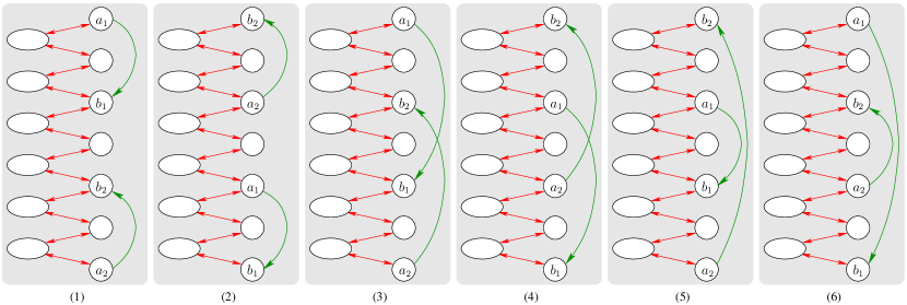
Figure 2: A conflict-cycle of type I can be formed for each of the six general cases as follows: (1)   $a_{1}\to_{X}b_{1}\to_{F}^{*}b_{2}\to_{F}a_{2}\to_{Y}b_{2}\to_{F}^{*}b_{1}\to_{F}a_{1}$,   (2)   $a_{1}\to_{X}b_{1}\to_{F}a_{1}\to_{F}^{*}a_{2}\to_{Y}b_{2}\to_{F}a_{2}\to_{F}^{*}a_{1}$,   (3)  $a_{1}\to_{X}b_{1}\to_{F}a_{2}\to_{Y}b_{2}\to_{F}^{*}b_{1}\to_{F}^{*}b_{2}\to_{F}a_{1}$,   (4)   $a_{1}\to_{X}b_{1}\to_{F}a_{2}\to_{F}^{*}a_{1}\to_{F}^{*}a_{2}\to_{Y}b_{2}\to_{F}a_{1}$,   (5)   $a_{1}\to_{X}b_{1}\to_{F}a_{1}\to_{F}b_{1}\to_{F}^{*}a_{2}\to_{Y}b_{2}\to_{F}^{*}a_{1}$,   (6)  $a_{1}\to_{X}b_{1}\to_{F}^{*}a_{2}\to_{Y}b_{2}\to_{F}a_{2}\to_{F}b_{2}\to_{F}^{*}a_{1}$.

Based on the above lemma, we propose the following algorithm to find a minimal type I conflict-cycle (if any). For all pairs of arcs $\langle e_{1},e_{2}\rangle\in X\times Y$, where $e_{1}=a_{1}\to b_{1}\in X$ and $e_{2}=a_{2}\to b_{2}\in Y$, first compute $a=\min\{a_{1},b_{1},a_{2},b_{2}\}$ and $b=\max\{a_{1},b_{1},a_{2},b_{2}\}$ and then test if there exists a path $a\to_{F}b$ from $a$ to $b$ using arcs all from $F$ (each taking $O(n)$ time). Among all those pairs that passed the test, the one that attains the smallest value of $(b-a)$ will be returned as a minimal type I conflict-cycle. Note that this algorithm can be executed in $O(n^{5})$ time since the total number of arc pairs is no more than $O(n^{4})$.

Consider now the whole execution of the algorithm Approx-MBVS. Note that two while loops of Approx-MBL cannot each be repeated more than $n$ times because we delete at least one vertex in $F$ for each minimal conflict-cycle $\mathcal{C}$ to be considered. Therefore, the algorithm Approx-MBVS (and hence Algorithm Approx-MBL) can be executed in $O(n^{7})$ time. The main result of this paper thus follows (the approximation ratio follows from Theorem 5.15).

Theorem 5.19

Algorithm Approx-MBL achieves an approximation ratio of $(m^{2}+2m-1)$ for the MBL problem and runs in $O(n^{7})$ time, where $m$ is the number of genetic maps used to create the input partial order and $n$ the total number of distinct genes appearing in these maps.

6 Conclusions

In this paper, we have studied the MBL problem in its original version, i.e., it assumes that gene strandedness is not available in the input genetic maps. We found that the approximation algorithm proposed in [3] for the MBL problem is not applicable here because it implicitly requires the availability of gene strandedness. Therefore, we revised the definition of conflict-cycle in the adjacency-order graphs, and then developed an approximation algorithm by basically generalizing the algorithm in [3]. It achieves a ratio of $(m^{2}+2m-1)$ and runs in $O(n^{7})$ time, where $m$ is the number of genetic maps used to construct the input partial order and $n$ the total number of distinct genes in these maps. We believe that the same approximation ratio also applies to the special variant of the MBL problem studied in [3], thereby achieving an improved approximation ratio over the previous one $(m^{2}+4m-4)$ given in [3]. In the future, it is very interesting to investigate whether an $O(m)$-approximation can be achieved for the MBL problem.

References

- [1] V. Bafna and P. A. Pevzner. Genome rearrangements and sorting by reversals. In SFCS ’93: Proceedings of the 1993 IEEE 34th Annual Foundations of Computer Science, pages 148–157, 1993.
- [2] Guillaume Blin, Eric Blais, Danny Hermelin, Pierre Guillon, Mathieu Blanchette, and Nadia El-Mabrouk. Gene Maps Linearization using Genomic Rearrangement Distances. Journal of Computational Biology, 14(4):394–407, 2007.
- [3] Laurent Bulteau, Guillaume Fertin, and Irena Rusu. Revisiting the minimum breakpoint linearization problem. In TAMC, pages 163–174, 2010.
- [4] Xin Chen and Yun Cui. An approximation algorithm for the minimum breakpoint linearization problem. IEEE/ACM Trans. Comput. Biol. Bioinformatics, 6(3):401–409, 2009.
- [5] Xin Chen and Jian-Yi Yang. Constructing consensus genetic maps in comparative analysis. Accepted by Journal of Comput. Biol., 2010.
- [6] Zheng Fu and Tao Jiang. Computing the breakpoint distance between partially ordered genomes. Journal of Bioinformatics and Computational Biology, 5(5):1087–1101, 2007.
- [7] Immanuel V. Yap, David Schneider, Jon Kleinberg, David Matthews, Samuel Cartinhour, and Susan R. McCouch. A Graph-Theoretic Approach to Comparing and Integrating Genetic, Physical and Sequence-Based Maps. Genetics, 165(4):2235–2247, 2003.
- [8] Chunfang Zheng, Aleksander Lenert, and David Sankoff. Reversal distance for partially ordered genomes. Bioinformatics, 21(suppl_1):i502–508, 2005.
- [9] Chunfang Zheng and David Sankoff. Genome rearrangements with partially ordered chromosomes. Journal of Combinatorial Optimization, 11(2):133–144, 2006.