A computer-simulated Stern-Gerlach laboratory

Abstract

We describe an interactive computer program that simulates Stern-Gerlach measurements on spin-$1/2$ and spin-1 particles. The user can design and run experiments involving successive spin measurements, illustrating incompatible observables, interference, and time evolution. The program can be used by students at a variety of levels, from non-science majors in a general interest course to physics majors in an upper-level quantum mechanics course. We give suggested homework exercises using the program at various levels. ©1993 American Association of Physics Teachers. Published in Am. J. Phys. 61 (9), 798–805 (1993), <http://dx.doi.org/10.1119/1.17172>.

I Motivation and Overview

Quantum mechanics is central to 20th century physics, yet instructors disagree strongly over how, and when, to teach this subject to students. A course in quantum mechanics for beginning students faces several obstacles: The full theory is horribly abstract and mathematical, while simplified presentations tend to be vague and misleading. The same hurdles are present, though perhaps less severe, at the start of an upper-level quantum mechanics course for physics majors.

Much of the math can be avoided, at least for a while, by starting with finite-dimensional spin systems.FeynmanLectures One disadvantage of this approach, however, is that it makes the subject even more abstract, as the measurable quantities are not as familiar as position and momentum. In principle, this problem could be solved by assigning laboratory exercises with Stern-Gerlach devices, but in practice such experiments are difficult and expensive to carry out.

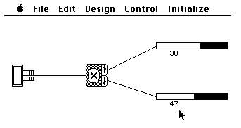
Figure 1: The simplest experimental arrangement, with a single Stern-Gerlach device and two counters. (This experiment is ready to run when the program starts.)

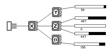
Figure 2: A much more complicated experiment, involving successive Stern-Gerlach devices and spin-1 particles.

This article describes a computer program, called Spins, that is designed to address these issues. A Stern-Gerlach laboratory is simulated on the computer screen (see Fig. 1), allowing the student to quickly design and run a number of experiments involving spin systems. As the experiment runs, simulated particles are sent through the devices one at a time, while the student watches the numbers on the counters increase. Multiple Stern-Gerlach devices, oriented in various directions, can be linked together in any order, and can be used to study spin-1 as well as spin-$1/2$ particles (Fig. 2). Interference can be studied by combining the beams emerging from one device and sending them into a second (Fig. 3). Time evolution can also be observed, using a device that simulates the effect of a uniform magnetic field (Fig. 4).

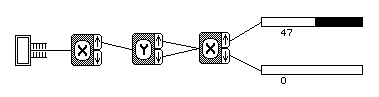
Figure 3: An interference experiment with spin-$1/2$ particles.

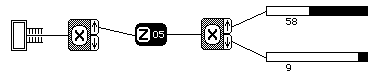
Figure 4: In this experiment, spin-1/2 particles with spin up in the $x$ direction are placed in a uniform magnetic field, oriented in the $z$ direction, for 5 time units. Then the $x$ components of their spins are measured.

The pedagogical values of the program are numerous. Most obviously, it gives students a concrete visual image to go with each of the concepts just mentioned. In addition, the program makes the statistical nature of quantum-mechanical predictions obvious. More generally, through designing and running their own experiments, students see the theory at work in a somewhat realistic setting, and learn to separate the arbitrary mathematical conventions from the unambiguous physical predictions.

Students at almost any level can use the program. Anyone with sufficient curiosity can play with it and try to invent a theory to explain the strange behavior of the particles. Students with some knowledge of geometry can arrive at a complete understanding of a restricted set of experiments with spin-$1/2$ particles. Introductory physics students can learn enough about complex numbers to understand spin-$1/2$ quantum mechanics in general, while upperclass physics majors can explore the full complexities of a nontrivial three-dimensional system.

Most of the rest of this article consists of guidelines and exercises written for users of the program. Since the program can be used at so many different levels, we are immediately faced with the question of who the users are. Sections II and III are written for students with no prior knowledge of physics and no mathematical background beyond plane geometry; Section II contains basic instructions, while Section III contains theoretical explanations and suggested homework exercises at this level. Section IV contains a brief discussion of uses for the program at more advanced levels, followed by an extensive set of advanced exercises. In Section V we add a few general comments for instructors, and briefly discuss the current implementation of Spins on the Macintosh.

II Basic Instructions

II.1 Getting started

Welcome to Spins, a quantum physics laboratory at your fingertips! When you start the program you see a diagram of a simple physics experiment (see Fig. 1). At the left is a device (we’ll call it a gun) that emits particles (call them atoms), one at a time. The atoms follow the line to the right, then enter another device, an X-analyzer, which deflects them either up or down. They leave the $X$-analyzer through one of two possible holes on its right side, then follow the paths shown into two counters. Physicists say that this experiment “measures” a property of the atoms called “spin in the $x$ direction”. Atoms coming out of the upper hole of the $X$-analyzer are said to have “spin up in the $x$ direction”, while those coming out of the lower hole are said to have “spin down in the $x$ direction”. For this particular type of atoms, only these two outcomes of the measurement are possible.

To start the experiment, choose ‘Go’ from the ‘Control’ menu.UINote Let it run for a while, then choose ‘Stop’ from the same menu. You can start and stop as many times as you like. You can reset the counters and start over by choosing ‘Reset’. If you want to run the experiment for a long time but don’t want to wait so long, choose ‘Do 1000’ or ‘Do 10000’, and the computer will send that many atoms through the apparatus very quickly, updating the counters when it is done.

You should see about half of the atoms ending up in each counter. Repeat the experiment several times, and convince yourself that although the numbers on the two counters are hardly ever exactly equal, the deviations from equality are in some sense “small” and “random”. A physicist would say that these atoms are equally probable to be found with their spins up or down in the $x$ direction.

This particular experiment gets tiresome before long, but you can create different (and much more interesting) experiments in several ways. First, put the cursor over the ‘X’ on the $X$-analyzer and click. The ‘X’ will change to a ‘Y’, and you have magically changed the $X$-analyzer into a new type of device, a $Y$-analyzer. Clicking again changes it into a $Z$-analyzer, then a $\theta$-analyzer, and finally back into an $X$-analyzer. Run the experiment again with the $Y$-analyzer (and the others if you wish), and see what happens.

To make a more complicated experiment you can send the atoms through two analyzers in succession. You can create more analyzers with the ‘New Analyzer’ command under the ‘Design’ menu. You can create more counters in a similar way. You can then move them around the screen with the mouse. (To move an analyzer, place the cursor in the gray region surrounding its letter; the cursor will take the form of crossed arrows. Press the mouse button, and drag the analyzer to its new location.) To draw lines connecting the components together, first press in the output end of one (the cursor will take the form of an arrow pointing to the right), then drag to the other and release. If you decide that you no longer need a component, you can select it (by clicking on it) and choose ‘Delete’ from the ‘Design’ menu.

Try designing some experiments of your own now, to get a feel for how to manipulate the components, and to learn more about how these atoms behave. Use only $X$- and $Y$-analyzers for now, to keep things simple. What happens when you run the atoms through two successive analyzers of the same type? What if the types are different? Keep looking for patterns until you think you can predict the outcome of any experiment built out of these two types of analyzers. Try to formulate a set of rules that would tell someone else what the outcome of any such experiment would be.

You may be wondering what these “analyzers” actually are, and how they would work in a real experiment. The details don’t matter, but you should know that a $Y$-analyzer is just an $X$-analyzer turned on its side. The $\theta$-analyzer is also the same apparatus, but you can turn it to any angle with the ‘Change Theta’ command on the ‘Design’ menu; an $X$-analyzer is the same as a $\theta$-analyzer turned to zero degrees, while a $Y$-analyzer is the same as a $\theta$-analyzer turned to 90 degrees. Try running some experiments to confirm this. Then try some other angles, and see if you can find a pattern.

The only other thing you need to know about the analyzers is that they contain no moving parts (each is actually no more than a strangely shaped magnet surrounding the path of the atoms); each analyzer always looks the same no matter which of its openings the atoms come out of. Similarly, the atoms themselves behave identically under all circumstances except when they are passed through one of the analyzers. There is no way to tell just by “looking” at an atom whether it will go up or down. Of course this does not necessarily mean that the atoms emitted from the gun are all identical; that is for you to decide, on the basis of your experiments.

II.2 Interference

Here’s a good experiment to try next (see Fig. 3). Connect the gun to an $X$-analyzer. Connect the up-output of this $X$-analyzer to a $Y$-analyzer. Then connect both outputs of this $Y$-analyzer to a second $X$-analyzer. Connect all remaining outputs to counters. Run the experiment in this configuration, then try disconnecting one of the two paths from the $Y$-analyzer to the final $X$-analyzer. First disconnect one, then the other, then try it again with them both connected. Can you explain the results? If the rules you formulated above do not give the correct prediction here, try to modify them to cover this experiment as well as the others. The phenomenon exhibited here is called “interference” by physicists, and is analogous to the interference of light passing through a double slit.

Since the atoms pass through the apparatus one at a time, you may wonder if it is possible to watch each atom as it goes through, to see which of the two paths it takes. You can do this, but not without modifying the analyzers. Select ‘Watch’ from the ‘Control’ menu. This attaches a light to each output opening of each analyzer; the light bounces off the atoms as they pass through the opening, causing a brief flash. Now repeat the experiment, and see what happens.

II.3 Additional commands

The program has several additional features, which allow you to build still more complicated experiments. Here is a brief summary of the menu commands.

The ‘Initialize’ menu determines how the gun works. Although the atoms coming out of it always look the same, they will behave differently if you choose a different “initial state”. You can choose three different initial states, but it’s up to you to determine how they differ. You can also choose ‘Random’, which randomizes the initial states.

The ‘Design’ menu lets you create another type of experimental device: a “magnet” (see Figure 4). Magnets come in four types, $X$, $Y$, $Z$, and $\theta$, just like analyzers. Each magnet has just one input and one output, so you can direct atoms through it and then use an analyzer to determine how they have been affected. The two-digit number on the magnet determines how much time the atoms spend inside (in very small units so that even 99 units of time is not long enough to noticeably slow down the experiment). Try setting up the experiment shown in Figure 4, with a $Z$-magnet between two $X$-analyzers. Increment the time (by clicking on the number) very gradually, and systematically investigate the magnet’s effect on the behavior of the atoms as they pass through the second analyzer. Caution: Experiments with magnets can be quite complicated. To understand the effect of magnets other than type $Z$ requires a substantial amount of mathematics.

You can experiment with a completely different type of atoms by choosing ‘3-State Spin’ from the ‘Design’ menu. When these atoms are sent through an analyzer they are found to bend in one of three different directions, so the analyzers are now provided with three output openings instead of just two. The numerical results of the experiments get much more interesting now, but with a bit of work you should still be able to find some patterns in the results (at least for $X$ and $Y$, and $Z$). Using magnets and $\theta$-analyzers in conjunction with the 3-state atoms is very interesting, but not recommended for beginners.

III Elementary Explanations and Exercises

III.1 The rules of quantum mechanics

Please don’t read on until you have performed several experiments and formulated your own set of rules for predicting how the atoms behave. You may be able to come up with a better set of rules than the ones given here.

Now that you’ve tried to understand the results of several experiments, you may wonder how physicists understand them. The short answer is, we don’t. The best we’ve been able to come up with is a fairly concise set of “rules” for calculating the (average) outcome of such an experiment. You can decide whether these rules shed any light on what is really going on.

The rules stated here are sufficiently general to cover experiments involving $X$, $Y$, and $\theta$-analyzers, as well as $Z$-magnets, for the 2-state spin system. The generalization to other experiments requires more mathematics, but the concepts are essentially the same.ClassNote

Rule 1: Physicists represent the “state” of an atom at any given time by an arrowArrowsVsSpinors drawn on a piece of paper (see Fig. 5). All allowable arrows have the same length (which we’ll take to be one “unit”), but they can point in different directions. Arrows that point in opposite directions ($180^{\circ}$ apart) represent the same physical state. Thus there are infinitely many possible states, corresponding to the infinitely many directions (from $0^{\circ}$ to $180^{\circ}$) in which the arrow can point.

Figure 5: We represent the state of an atom by an arrow drawn on a piece of paper. The length of the arrow is one “unit”, while the direction of the arrow depends on the state in question. Arrows pointing in opposite directions represent the same state.

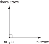
Figure 6: An analyzer corresponds to a pair of unit-length arrows, perpendicular to each other. (The directions of the arrows depend on which analyzer they represent.)

Rule 2: Similarly, we represent each analyzer by a pair of perpendicular, unit-length arrows, whose tails coincide (see Fig. 6). One of these arrows corresponds to the result “up” for that analyzer, while the other arrow corresponds to the result “down”. We will call the arrows the up arrow and the down arrow. (Note that these arrows need not, and usually do not, point up or down on the sheet of paper. In general, the direction of an arrow on the paper has no direct relation to the physical orientation of the analyzer.) The point where the tails of the up and down arrows meet is called the origin.

Rule 3: When an atom passes through an analyzer, it has a certain probability of going up, and a certain probability of going down. We usually can’t predict which it will do; we can only calculate the probabilities. To compute the probability of going up, you first draw the arrow corresponding to the atom’s current state, and the two arrows corresponding to the analyzer, on a single piece of paper with all their tails together at the origin (see Fig. 7). Suppose first that the angle between the state arrow and the up arrow is less than $90^{\circ}$. You then draw a new line from the tip of the state arrow, which meets the analyzer’s up arrow at a right angle. Measure the distance from the origin to this perpendicular intersection of the new line and the up arrow. This distance is called the amplitude for the atom to go up. The probability for the atom to go up is the square of the amplitude. If the angle between the state arrow and the up arrow is greater than $90^{\circ}$, you must first rotate the state arrow by $180^{\circ}$, then follow the same procedure; in this case the amplitude is the negative of the distance from the origin to the perpendicular line (but the probability, being the square of the amplitude, is still positive). The probability to go down is computed in a similar way, using the analyzer’s down arrow. Since the state arrow has unit length, the Pythagorean theorem guarantees that the two probabilities add up to 1.

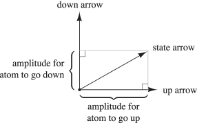
Figure 7: To determine the amplitudes for the atom to go up and down, use this geometrical construction.

Rule 4: When the atom leaves the analyzer, its arrow changes abruptly. If it went up, its new arrow is the same as the analyzer’s up arrow; if it went down, its new arrow is the same as the analyzer’s down arrow.

Rule 5: In experiments where beams are recombined (as in Fig. 3), we must use more care in converting amplitudes to probabilities. Consider each path that the atom could take in order to produce a certain final outcome, and compute the amplitude for each path by multiplying together the amplitudes for each step along the path. Then compute a total amplitude for the final outcome by adding together the amplitudes for all paths. The probability of the outcome is the square of this total amplitude. (When there is only one possible path, this method gives the same result as computing the probability separately for each step, as described in Rule 3.)

Rule 6: A $Z$-magnet causes the atom’s arrow to rotate in the plane of the paper at a uniform speed, as long as the atom is inside the magnet.

You may have noticed that these rules are extremely abstract. They give only a general framework for describing quantum mechanical experiments, without any specific prescriptions for which arrows we should associate with which states. That is because the specifics are, to a certain degree, arbitrary. The rules assert that we can come up with some set of arrows to associate with the various states and analyzers, and that once we do so, the outcomes of all experiments will be as predicted. The following exercises should clarify where the arbitrariness ends and the predictions begin.

III.2 Exercises with the 2-state spin system

Now that you know the rules, you should be able to work the following exercises. Once you’ve done so, you will understand this system as well as any physicist.

Figure 8 shows the up and down arrows of the $X$-analyzer. The directions of these arrows have been chosen arbitrarily, subject to the constraint that they are perpendicular to each other. Also shown in the figure is a circle whose radius is 1 unit;FigureSize all other arrows, whatever they represent, must lie with their tails at the origin and their tips somewhere on this circle.

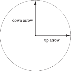
Figure 8: Here we have chosen the directions of the up and down arrows of the $X$-analyzer arbitrarily, subject to the constraint that they be perpendicular to each other. The circle is for reference: all arrows must have their tails at the center and their tips on this circle.

Set up the simple experiment shown in Fig. 1, and choose ‘Unknown #3’ from the ‘Initialize’ menu. By running this experiment several times, determine the probabilities for the atoms to go up and down. Take the square root of each probability to determine the amplitudes for each result, remembering that either amplitude could be positive or negative. Knowing these amplitudes, you can almost determine the state arrow of the atoms: you should be able to narrow it down to four possibilities. Sketch the four arrows lightly on the figure.

Add a second $X$-analyzer between the gun and the first $X$-analyzer (see Fig. 9), and run the experiment. Repeat the experiment with the down output (rather than the up output) of the first analyzer connected to the input of the second. Also repeat the experiment with both $X$-analyzers changed to $Y$-analyzers. Is the behavior of this system consistent with Rule 4? Explain your answer carefully.

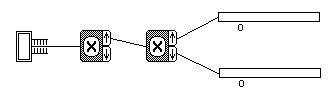
Figure 9: An experiment to test Rule 4, ready to run. (The outcome will be that all the atoms end up in the top counter.)

Repeat the above experiment, but this time with one $X$-analyzer and one $Y$-analyzer (in various combinations). Using the results of these runs, find the directions of the up and down arrows of the $Y$-analyzer. Again, you should find several possible directions for the arrows. Choose one set of arrows arbitrarily, and draw them on the figure.

Now use an experiment with a single $Y$-analyzer to narrow down the choices for the initial arrow. There should be two candidate arrows left, but they should point in opposite directions. Since Rule 1 says that arrows pointing in opposite directions represent the same physical state, either of these arrows is correct.

Set up the interference experiment as described in Section 2. Is this experiment consistent with Rule 5?

Set up an experiment with a $Z$-magnet between two $X$-analyzers. Rule 6 says that the magnet will make the atom’s state arrow rotate at a fixed rate. By what angle does it rotate for each unit of time spent in the magnet? What time setting corresponds to a full 360-degree revolution of the arrow? Try to design an experiment that will tell you in which direction the arrow rotates.

IV Guidelines for More Advanced Uses

IV.1 Introductory physics courses

The student instructions in Sections II and III can easily be adapted for use in an introductory physics course, where students have more mathematical knowledge and vocabulary. The “arrows” can become “vectors”, and the geometrical construction of Rule 3 can become a dot product. This makes it possible to give purely algebraic rules, although the geometric interpretation can still be helpful to students. Anyone familiar with sines and cosines will have little difficulty determining the state vectors associated with the $\theta$-analyzer. To include rules for the $Z$-analyzer one must introduce complex numbers,BasisChoice for which the geometric interpretation fails.

The time-evolution postulate (Rule 6) could be replaced by the full time-dependent Schrödinger equation, although this requires some mathematical sophistication on the part of the students. An alternative approach in an introductory course is to give the following algorithm for determining the time evolution of a given initial state: Write the initial state vector as a linear superposition of the two orthogonal vectors associated with the direction of the magnet, then multiply each term by a factor $\exp(-i\omega t)$, where $\omega$ equals some constant for the “up” piece, and minus the same constant for the “down” piece. After determining the correct constant, students can predict the outcome of any measurement performed on atoms that have passed through a magnet.

IV.2 Upper-level physics courses

In an upper-level quantum mechanics course for physics majors, students are generally introduced to all the mathematical machinery of hermitian matrices, eigenvalues and eigenvectors, and the time-dependent Schrödinger equation. For the purpose of using this program, they should also be taught some version of the postulates of quantum mechanics, analogous to those presented in the previous section. This allows them to deal with the 3-state system in all its complexity. The following exercises illustrate some of the possibilities. Many of them are analogous to the elementary exercises of the previous section, but some are considerably more intricate.

IV.3 Exercises for advanced students

We will adopt the convention that all vectors are expressed in terms of the “eigenbasis” of the $X$-analyzer. This means that the eigenvectors of the $X$-matrix are $(1,0,0)$, $(0,1,0)$, and $(0,0,1)$. (Note that these vectors are all normalized and mutually orthogonal.) We will take the eigenvalues of the matrix to be $1$, $0$, and $-1$, corresponding to up, 0, and down, respectively. Associating the eigenvectors with the eigenvalues is also a matter of convention; we will take the eigenvectors to correspond to the eigenvalues in the order in which they are listed above. Given these conventions, what is the $X$-matrix?

Choose ‘3-State Spin’ from the ‘Design’ menu, and ‘Unknown #1’ from the ‘Initialize’ menu. Use the $X$-analyzer to find the state vector of this initial state. You will only be able to determine the components of the vector to within complex factors of unit modulus (why?). Since vectors that differ by an overall constant factor represent the same physical state, we can choose the convention that the first component be real and positive. There are still unknown factors in the other two components, however. Assume for now that the components of this vector are all real. Then the only ambiguities are in the signs of the second and third components.

Hints: All components of vectors and matrices used here can be written as simple fractions of small integers (like $1/2$), or as square roots of such simple fractions. It may help you to know that if you perform an experiment $N$ times, and the probability of a certain result is $p$, the number of times that you actually obtain that result can differ from the expected number $Np$ by as much as about $2\sqrt{Np(1-p)}$. (More precisely, the standard deviation of the distribution is $\sqrt{Np(1-p)}$; the probability of being off by more than two standard deviations is very small, about 5%.)

Is the behavior of this system consistent with the “collapse” postulate? Perform successive measurements with both $X$ and $Y$ analyzers to justify your answer.

Find the eigenvalues and eigenvectors of the $Y$-matrix. Once again you will not be able to determine them uniquely. Use the convention that all components be real, and that the first component of each, as well as the remaining components of the eigenvector corresponding to the eigenvalue $+1$, be positive.

These conventions for the $Y$-matrix are sufficient to determine the unknown signs in the components of the initial state. What are they?

Prove the identity $Y=MXM^{\dagger}$, where $X$ and $Y$ are the matrices corresponding to the $X$ and $Y$ analyzers, $M$ is a matrix whose columns are the eigenvectors of $Y$, and $M^{\dagger}$ is the conjugate transpose of $M$. This identity gives you an easy way to find the $Y$-matrix (it can also be found by brute force, by solving a system of linear equations). What is the $Y$-matrix?

The $\theta$-analyzer is just an $X$-analyzer rotated by an angle $\theta$. (A $Y$-analyzer is a $\theta$-analyzer with $\theta$ = 90 degrees.) This means that the quantity measured by $\theta$ can be expressed as $X\,\cos\theta+Y\,\sin\theta$. The postulates say that the $\theta$-matrix is given by this same function of the $X$ and $Y$ matrices. What is the $\theta$-matrix? What are its eigenvalues and eigenvectors? Connect one of the outputs of an $X$-analyzer to the input of a $\theta$-analyzer, and calculate the probabilities for obtaining the three possible outcomes of the $\theta$-measurement, as a function of $\theta$. Verify your predictions by running the experiment for several different values of $\theta$.

A magnet causes the state vector to evolve according to the time-dependent Schrödinger equation. The solution of this equation can be written formally as $\psi(t)=\exp(-iHt)\psi(0)$. Normally this expression is not very useful, since it is usually impossible to evaluate the exponential of the matrix. But since we are working with very simple $3\times 3$ matrices, we can use this expression directly. The matrix $\exp(-iHt)$ is called the propagator, and denoted by $U(t)$. We will try to determine $U(t)$ (and hence $H$) for the $Z$-magnet in the 3-state system.

Since we are using the eigenvectors of the $X$-matrix as our basis, the matrix elements of $U(t)$ are found most easily by sending atoms that are in $X$-eigenstates into the magnet, then measuring $X$ again when they come out. So connect the gun to an $X$-analyzer, one output of this analyzer to a $Z$-magnet, the output of the magnet to a second $X$-analyzer, and all three outputs of this analyzer to counters. Choose any initial state that gives you nonzero counts. Increment the time on the magnet slowly, and record the number of atoms in each counter after a reasonably long run (1000 atoms or so) for each value of the time. Graph the relative probability for ending up in each counter as a function of time. Repeat the whole process using each of the three outputs of the first $X$-analyzer.

You should now have nine graphs. For what value of the time does the atom have the same state vector coming out of the magnet that it had going in? (That is, for what value of $t$ does $U(t)=1$?) Each graph represents the square of one element of the $3\times 3$ matrix $U(t)$ (why?). Try to guess the functional form of the curve for each of your graphs. (Hints: It is easier to guess the functional form of the square root of the probability. You will get simple functions involving sines and cosines; for example, one of the matrix elements is $(1+\cos\theta)/2$.) Remember that for any given experiment, the sum of the three probabilities you measured must be 1. Do the functions you guessed satisfy this constraint? Given the nine probabilities, the elements of the matrix $U(t)$ are still unknown up to factors of unit modulus. To make your job easier, we have chosen the matrix elements of $H$ to be pure imaginary, and hence $U(t)=\exp(-iHt)$ is pure real. Given this information, you now know the matrix elements of $U(t)$ except for possible factors of $-1$.

You can determine the nine unknown signs in $U(t)$ with very little difficulty. First note that $U(t=0)$ must equal 1; this determines three of the nine signs. Five of the remaining six can be found by changing one or the other (you will have to do both, one at a time) of the $X$-analyzers into a $Y$-analyzer. Find a time setting on the magnet that changes a pure $X$ eigenstate into a pure $Y$ eigenstate, or vice versa. The conventions used above for the $Y$ eigenstates will determine the unknown signs. The final unknown sign can be found by expanding $U(t)$ as a power series in $t$ and recognizing the linear term as $-iHt$. The fact that $H$ is Hermitian gives one more relation among the signs. Write down your final expression for $U(t)$.

The expression for $H$ you just obtained still contains an unknown overall constant, which you can make anything you want by re-defining the standard unit of time. (In other words, making the magnet twice as strong has the same effect as leaving the atoms inside twice as long.) Use the following convention: Let $t$ be the time variable that appears in the Schrödinger equation, let $n$ be the number displayed on the magnet, and let $N$ be the number on the magnet that corresponds to one full cycle (so that $U(n=N)=1$). Then define $t=2\pi(n/N)$. Given these conventions, what is $H$? As a check, you should find that the eigenvalues of $H$ are $1$, $0$, and $-1$. Finally, try to verify explicitly that $U(t)=\exp(-iHt)$. (Hint: One way to do this is first to pretend that $H$ is the diagonal matrix diag$(1,0,-1)$, and find an expression for $\exp(-iHt)$ as a linear combination of 1, $H$, and $H^{2}$. Then note that there exists a matrix $M$ such that $M^{\dagger}M=1$ and $M^{\dagger}HM={\rm diag}(1,0,-1)$, and use this fact to prove that your expression is correct even though $H$ is not diagonal.)

It so happens that $H$ is identical to the matrix of the $Z$-analyzer. Find its eigenvectors, and verify this by performing some experiments.

Referring back to your data for $X$-analyzers before and after the magnet, for the case where the initial $X$-analyzer gave the result ‘up’, make a graph of the expectation value (i.e., weighted average) of the final $X$-measurement as a function of time spent in the magnet. Verify that the expectation value is $\psi^{\dagger}X\psi$, where $X$ is the $X$-matrix and $\psi$ is the state vector of the atom as it leaves the magnet. Change the final $X$-analyzer to a $Y$-analyzer, and find an expression for the expectation value of $Y$ as a function of time for the same initial state ($X$ up). Verify Ehrenfest’s theorem, which says that for any observable $A$, $d\langle A\rangle/dt=-i\langle AH-HA\rangle$, where $\langle A\rangle$ denotes the expectation value of the observable $A$ (and similarly for the observable $AH-HA$). Note that if we consider only expectation values, an atom behaves like a classical magnet, initially pointing in the $X$-direction, spinning about its axis, and precessing in the presence of a magnetic field that points in the $Z$-direction. In other words, the expectation values of quantum observables behave as classical observables.

V Additional Comments

The sets of example exercises given in Sections III.B and IV.C are both too short and two long. They are too short in the sense that they could hardly stand alone in this form—they would have to be amplified and adapted for the specific needs of any particular course. But they are also too long, since working either set of exercises could take students as long as two weeks. The minimum time investment required before the program’s educational benefits become significant is probably one week. At least in a course for beginning students, this is a lot of time to spend on the quantum mechanics of spin systems, a subject that has little practical “use”.

Although this program simulates a quasi-realistic set of experiments, it is certainly not intended as a substitute for real-life laboratory experience. In particular, some limited experiments of this type can be performed with polarized light and calcite crystals. We hope that the real experiments and the simulated ones can complement each other.

The current incarnation of Spins is written in Pascal and runs only on the Macintosh personal computer. This program is currently available directly from Daniel Schroeder.HowToGetSpins

The source code for the Macintosh version of Spins is quite long (nearly 3000 lines), for two reasons. First, the Pascal language is not ideally suited to working with the complex numbers, vectors, and matrices of quantum theory, so the implementation of the basic quantum mechanical rules is not very elegant. Second, a great deal of code is needed to implement the graphical user interface. Unfortunately, none of the user interface routines are portable to other machines. With sufficient time, however, one could create an equivalent program for any machine with a graphical user interface. The authors would be happy to assist anyone who is seriously interested in undertaking such a project.HowToGetSpins

On systems with a traditional “command-line” user interface, one can easily implement a more limited version of the program. The experiment would proceed as a dialog such as the following:

User: prepare 1000
Computer: 1000 atoms are being fired from the gun.
U: measure x
C: Results of X measurement: 476 up, 524 down.
U: select up
C: You have selected 476 atoms with X up.
U: measure y
C: Results of Y measurement: 261 up, 215 down.
etc.

Here the program merely keeps track of the current state vector of the system (an array of two or three complex numbers), dots this vector into the appropriate eigenvectors to determine the probabilities of all possible outcomes, and then generates a random number between 0 and 1 for each atom to determine the outcome of the measurement. When the user selects a subset of the atoms for a further measurement, the current state vector is set equal to the appropriate eigenvector, according to Rule 4. An implementation of this sort obviously lacks visual images, and would make interference experiments difficult or impossible, but most of the exercises described in the previous sections could still be carried out, with similar benefits to the student. The earliest version of the Spins program was of this type. This version has been used in a sophomore-level class, and students found that even this crude version helped make the postulates of quantum mechanics seem more concrete.

- (1) This approach has been taken by several authors, for instance, Richard P. Feynman, Robert B. Leighton, and Matthew Sands, The Feynman Lectures on Physics (Addison-Wesley, Reading, MA, 1965), vol. 3, ch. 5.
- (2) These instructions are written for the Macintosh implementation of the program, and assume that the user is familiar with the rudiments of the Macintosh user interface: using the mouse to select menu items and to “click”, “press”, “drag”, and “release”. A brief explanation of these terms should be included in the instructions for students.
- (3) The rules stated here are of course much too terse to be absorbed in a single reading. We assume that this material would be presented and discussed in class.
- (4) For students with a limited mathematical background, this geometrical representation using “arrows” is much more accessible than the usual algebraic representation. For the benefit of instructors, however, we point out that a unit-length arrow is completely equivalent to a normalized two-component spinor. In the exercises in Section III.B we will use the spinors and to represent spin up and down in the direction, and and (in either order) to represent spin up and down in the direction. The eigenstates of the -analyzer would then be represented by complex spinors, for which the geometrical picture breaks down. This is why we avoid -analyzers at this level.
- (5) To save space, the figure is reproduced here at a very small scale. In practice it is probably best to give the student a worksheet on which the figure occupies most of a page; a scale of 10 cm for the unit-length arrows works nicely. The instructions can then be made more concrete by replacing units with centimeters.
- (6) In these guidelines we have chosen to use a basis where the spin- operator is diagonal, rather than as is usually done. For beginning students this choice seems more natural. All experimental outcomes are of course independent of basis.
- (7) Updated information on obtaining the Spins program as of 2015: The original Mac Classic version of Spins is still available at <http://physics.weber.edu/schroeder/software/>, but almost nobody still has a computer that can run it. Fortunately, Spins has been ported to Java by groups at Oregon State University and Davidson College; the latest Java version is available at <http://www.physics.orst.edu/~mcintyre/ph425/spins/index_SPINS_OSP.html>. Finally, author TAM has created a more limited version of Spins in Xojo, with compiled versions that run on Mac OSX, Windows, and Linux; these versions are posted at <http://www.physics.pomona.edu/sixideas/sicpr.html>.