Parallelized Traveling Cluster Approximation to Study Numerically
Spin-Fermion Models on Large Lattices

Abstract

Lattice spin-fermion models are important to study correlated systems where quantum dynamics allows for a separation between slow and fast degrees of freedom. The fast degrees of freedom are treated quantum mechanically while the slow variables, generically refereed to as the “spins”, are treated classically. At present, exact diagonalization coupled with classical Monte Carlo (ED+MC) is extensively used to solve numerically a general class of lattice spin-fermion problems. In this common setup, the classical variables (spins) are treated via the standard MC method while the fermion problem is solved by exact diagonalization. The “Traveling Cluster Approximation” (TCA) is a real space variant of the ED+MC method that allows to solve spin-fermion problems on lattice sizes with up to $10^{3}$ sites. In this publication, we present a novel reorganization of the TCA algorithm in a manner that can be efficiently parallelized. This allows us to solve generic spin-fermion models easily on $10^{4}$ lattice sites and with some effort on $10^{5}$ lattice sites, representing the record lattice sizes studied for this family of models.

I Introduction

The rich physical properties displayed by many materials arise from strong correlations among multiple degrees of freedom Dagotto (2005); Tokura and Nagaosa (2000). Studying theoretically these materials has been a long standing challenge for materials theory since treating those coupled multiple degrees of freedom (DOF), such as the spin, charge, orbital, and lattice, on equal footing in a model Hamiltonian calculation is extremely difficult. As a consequence, accurate approximations that render such complex problems more tractable have always been of considerable interest. Dynamical Mean Field Theory Georges et al. (1996), Determinant Quantum Monte Carlo Blankenbecler et al. (1981); White et al. (1989); Paiva et al. (2010), and the Density Matrix Renormalization Group Schollwöck (2005) are some of those approximations that have led to important insights into the physics of correlated materials. Another useful approximation is to exploit the relative slow dynamics of some degrees of freedom as compared to others. As discussed below, this approach allows for the modeling of some complex materials with relative ease and on reasonably larger lattice sizes.

In materials such as the manganites Salamon and Jaime (2001); Tokura (2006), double perovskites Serrate et al. (2006), rare earth nickelates Medarde (1997); Gou et al. (2011), and others, the slow and fast separation is a good approximation. For example, in the manganites, the electrons in the $e_{g}$ orbitals have faster dynamics as compared to the dynamics of the localized $t_{2g}$ electrons and also compared to the Jahn-Teller and breathing mode phonons Salamon and Jaime (2001); Dagotto et al. (2001). This allows for a separation between “fast” and “slow” DOF. The quantum+classical approach treats the slow variables in the strict adiabatic limit, i.e., classically. Generically the slow variables that are considered classically are called “spins” and for this reason the models are commonly referred to as “spin-fermion” models.

The main advantage of this approximation is that the original fully interacting quantum many body problem can be mapped into a problem of noninteracting fermions coupled with, in general, spatially fluctuating classical fields. In the past, such classical+quantum approaches have been extensively used. Some well known methods in this context include the study of electron-phonon systems Migdal (1958); Kabanov and Mashtakov (1993), the Born-Oppenheimer approximation Born and Oppenheimer (1927), and the Car-Parrinello method Car and Parrinello (1985). Spin-fermion models for the manganites Dagotto et al. (2001); Yunoki et al. (1998); Moreo et al. (1999); Kumar and Majumdar (2006a); Dong et al. (2008, 2009); Liang et al. (2011); Şen et al. (2012), double perovskites Sanyal and Majumdar (2009); Erten et al. (2011), nickelates Johnston et al. (2014); Park et al. (2012), copper based high temperature superconductors Buhler et al. (2000a, b); Moraghebi et al. (2001, 2002a, 2002b), BCS superconductors Mayr et al. (2005); Alvarez et al. (2005); Mayr et al. (2006); Alvarez and Dagotto (2008), and the recently discovered iron superconductors Yin et al. (2010); Lv et al. (2010); Dagotto et al. (2011); Liang et al. (2013, 2012, 2014) have all exploited the slow and fast variables to considerable success.

Solving such spin-fermion models entails the search for the optimal configurations of the classical DOF that minimize the free energy. To achieve this goal, first the fermionic problem is diagonalized for a fixed configuration of the classical DOF and the energy is computed. The classical variables are then updated and the energy is recalculated in the updated background. The updates are accepted or rejected via the Metropolis algorithm. Finally the procedure is repeated until thermal equilibrium is reached and observables can be measured with reasonable accuracy.

This Exact Diagonalization + Monte Carlo (ED+MC) approach is free from the “sign problems” suffered by Quantum Monte Carlo methods and it can also include the study of long range spatial correlations unlike simple DMFT approaches. Over the years the ED+MC method has enjoyed considerable success in understanding correlated materials phenomena where the separation of slow and fast DOF is possible Dagotto et al. (2001). However, even after the considerable numerical simplification due to the quantum+classical treatment, the ED for the fermion problem still has to be carried out at every update of the classical fields resulting in thousands of diagonalizations at every temperature where the calculation is performed. Furthermore, the simulated annealing from high to low temperatures, which is often required to avoid being trapped in metastable states, requires sequential temperature steps. All these steps amount to a prohibitively large number of diagonalizations to be performed in a standard ED+MC calculation. This typically limits the accessible lattice or system sizes that can be solved using ED+MC to $\sim 10^{2}$.

The ability to solve such spin-fermion problems on larger systems is needed to address issues such as large length scale phase separation tendencies, to achieve accurate estimations of thermodynamic order and transport properties with small size effects, and to be able to perform reliable finite-size scaling analysis. Moreover, studies of the iron based superconductors have pointed out the need to study spin-fermion and Hubbard-like models incorporating multiple orbitals Raghu et al. (2008); Johnston (2010); Stewart (2011); Dai et al. (2012); Dagotto (2013). This task is challenging even on small system sizes due to large Hilbert spaces. In these regards the simple “Traveling cluster approximation” (TCA) Kumar and Majumdar (2006b) is an important step forward as it allows access to system of $\sim 10^{3}$ sites. This approximation is discussed below. In this publication, we present an alternate way to organize the TCA algorithm that allows for massive parallelization of the method. As a result, the calculation of spin-fermion models can now be performed on system sizes up to $\sim 10^{5}$ sites. Additionally, as discussed later, in the present generalization very large traveling clusters can be used for the TCA calculation. The small size of the traveling clusters has, till now, remained a limitation of the TCA approach.

Below we describe the parallelization scheme and benchmarks that we developed. As discussed in the text, techniques of the nature developed here will be instrumental in addressing problems in multiband Hubbard models as well.

The paper is organized as follows. In section II, we explain the TCA technique and compare it with ED+MC. In section III, we discuss our approach for parallelizing the TCA algorithm. In section IV, we present benchmarking results and in section V we provide some physically relevant results for the one orbital Hubbard model both in two and three dimensions and compare them with existing literature. In sections VI and VII, we discuss some pertinent numerical issues and in section VIII, we present the conclusions of the manuscript.

II Traveling Cluster Approximation

Let us begin by briefly discussing the basics of the ED+MC and TCA approaches.

a. ED+MC : As mentioned before, the spin-fermion model consists of a classical component and a quantum component. A Hamiltonian for spin-fermion models define the coupling between the classical DOF and the electrons and among the classical variables themselves. In usual ED+MC approaches, the classical variables at each site are updated one at a time and the energy of the system is calculated by diagonalizing the Hamiltonian and adding the classical contribution. This energy difference, before and after the update at a site, is used to accept or reject the proposed update. The process is then repeated over all of the sites visiting them either serially or randomly. This constitutes a single system “sweep”. The combined algorithm of ED+MC is numerically rather costly, since the exact diagonalization must be performed at every step and the cost scales as $\mathcal{O}(N^{3})$ with $N$ the number of lattice sites. Additionally, with a sequential system sweep, the cost of a Monte Carlo system sweep scales as $N^{4}$ at each temperature.

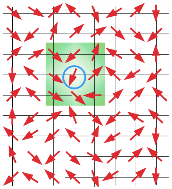
Figure 1: Two dimensional schematic of the TCA approach. Here a $N=8^{2}$ lattice is displayed with classical DOF at each site, represented by the red arrows. The Hamiltonian defines the coupling of the classical spins with the itinerant electrons that are delocalized on the lattice. The TCA algorithm consists of proposing an update at a site (encircled in blue) for the classical spins. The update is accepted or rejected based on the energy of a cluster built around that site, indicated in green. Here the cluster size is $N_{c}=9$. In a system sweep, the above procedure is carried out by visiting each site of the system sequentially.

b. TCA scheme: To reach reasonably large system sizes, a real space variant Kumar and Majumdar (2006b) of the ED+MC approach has been developed. As will be discussed below, this allows for a linear scaling with the system size, $N$, as opposed to the $N^{4}$ scaling of the computational cost with ED+MC.

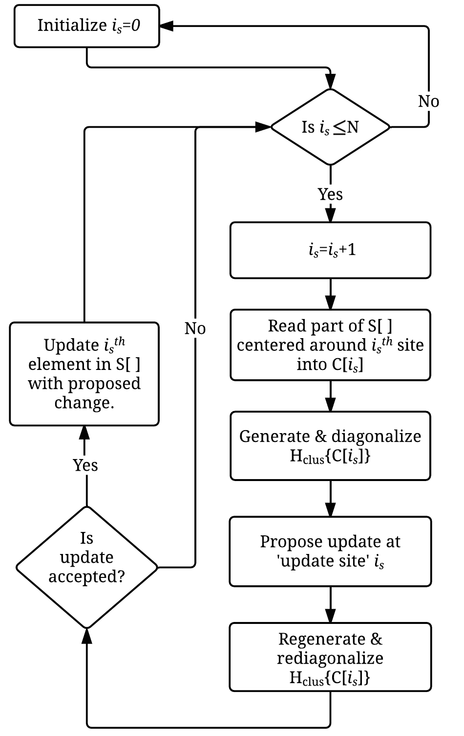
Figure 2: The flowchart for a single sequential Monte Carlo system sweep in the TCA approach. Here, we consider a lattice of $N$ sites. $S[~{}]$ is an array containing the classical DOF at all the $N$ sites. $C[i_{s}]$ is an array of size $N_{c}$ that reads in the classical DOF from $S[~{}]$ around the “update site” labeled by $i_{s}$. The loop over $i_{s}$ runs over all the $N$ sites of the system, ensuring that the cluster is built around all the sites sequentially and that an update is proposed at each site. The flowchart is discussed in the text.

In the TCA scheme one defines a region (cluster) around the site where a MC update is attempted. The cluster has a linear dimension $L_{c}$. Then, in a two dimensional square lattice, for example, the number of sites in the cluster is $N_{c}=L_{c}^{2}$. Such a cluster is shown in Fig. 1. The cluster is built around a site called the “update” site that it is encircled in blue. In this example $N_{c}=9$. The key difference with ED+MC is that the proposed update is accepted or rejected on the basis of the energy difference of the cluster and not the full system. As a result one needs to diagonalize only the cluster Hamiltonian which costs $N_{c}^{3}$ as opposed to $N^{3}$ for the full system diagonalization in ED+MC.

The analytical basis for the approximation of using a smaller cluster for the annealing process lies in the principle of “nearsightedness” of electronic matter, as discussed by W. Kohn Kohn (1996); Prodan and Kohn (2005). Furthermore, the method has been extensively tested and benchmarked in numerical studies Kumar and Majumdar (2005, 2006a). Consequently, in this paper we will assume the validity of the approximation without further discussion. The above update scheme is sequentially employed at every site of the system. The cluster of size $N_{c}$ is built around every site where the update is attempted, hence the name “Traveling” cluster approximation. Thus, within TCA, and at each temperature, the computational cost of ED for a system with $N$ sites is $\mathcal{O}(N_{c}^{3})$ and the cost of a full sweep of the lattice is $NN^{3}_{c}$ or linear in $N$ as opposed to $N^{4}$.

Many thousand MC system sweeps are performed at every temperature and for each temperature a large number of annealed classical configurations are stored. These are later used to construct and diagonalize the full system if it is necessary for calculating the desired output quantities. They are also useful for studying correlations among the classical variables.

As discussed in the original TCA paper Kumar and Majumdar (2006b), the geometry of the cluster is chosen to be the same as the system. Furthermore, one has to impose periodic boundary conditions on the cluster while calculating energies. These conditions ensure that in the limit of cluster sizes approaching the actual system size, the spectrum becomes identical. The periodically identified cluster can be considered to be an independent ensemble in contact with the full system where equilibrium is maintained in a grand canonical framework. An important aspect of this setup is that any site on the cluster can be chosen as the “update site”. In Fig. 1 we show this update site to be equidistant from all the edges. However, any other site, for example, the one in the top left corner, is also a equivalently good choice. This equivalence has been tested in many numerical studies Kumar and Majumdar (2006b, 2005, a) and we also checked numerically the same concept in the context of the Holstein model in section VII.

c. TCA flowchart: We end this section with the TCA algorithm, and the corresponding flowchart is presented in Fig. 2. In the flowchart the following nomenclature is used, and the same will be used for discussing the PTCA approach as well. We consider a system with $N$ sites. $S[~{}]$ is an array containing the classical variables at each site and it has the length $N$, assuming one classical variable per site. $H_{full}\{S[~{}]\}$ is the Hamiltonian for the full system, generated from the classical variables in $S[~{}]$. The array $C[i_{s}]$ is of length $N_{c}$ and it is the array holding the classical DOF at the cluster sites built around the $i_{s}^{th}$ site of the system. So this array reads the relevant part of $S[~{}]$. For example, in Fig. 1 $C[i_{s}]$ will read in, from $S[~{}]$, all classical variables that are at the lattice sites covered in the green square. From this setup the cluster Hamiltonian, $H_{clus}\{C[i_{s}]\}$, is constructed around the $i_{s}^{th}$ site. The $i_{s}^{th}$ site, where the update is proposed and around which the cluster is built, is referred to as the “update site.” With these notations, the following are the main steps explaining the TCA flowchart presented in Fig. 2.

1. In a single Monte Carlo system sweep, the index $i_{s}$ loops over all $N$ sites of the full system. Around each of the sites, $i_{s}$, a cluster will be built one at a time, traveling sequentially, as $i_{s}$ sweeps over the full lattice.

   1. $C[i_{s}]$ reads part of $S[~{}]$ around the site $i_{s}$.

   2. $H_{clus}\{C[i_{s}]\}$ is generated and diagonalized.

   3. The classical DOF is randomly modified at site $i_{s}$.

   4. $H_{clus}\{S[~{}]\}$ is generated with the update and rediagonalized.

   5. A Metropolis algorithm decides if the proposed update is accepted or not.

   6. If accepted the $i_{s}^{th}$ element in $S[~{}]$ is changed to the updated value.

2. The above process is repeated for all sites of the system.

III Scheme for parallelization

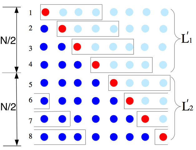
Figure 3: One dimensional example using $N=8$ and $N_{c}=4$. The light blue sites are the un-updated sites. The red site is chosen to be the site where the update is attempted (update site). The clusters are indicated by the boxes. The different rows present the cases of the cluster traveling sequentially from left to right during a single system sweep. The blue sites indicate the sites where an update has been attempted. The system and cluster both have periodic boundary conditions. For rows 1 through 5, the clusters are built based on the original (un-updated) classical variable configurations and can be constructed simultaneously instead of serially as in TCA. For rows 6 through 8, the clusters require the results of the update attempts on sites 1 through 3, respectively. So these clusters have to wait till row 4 and then can be built simultaneously.

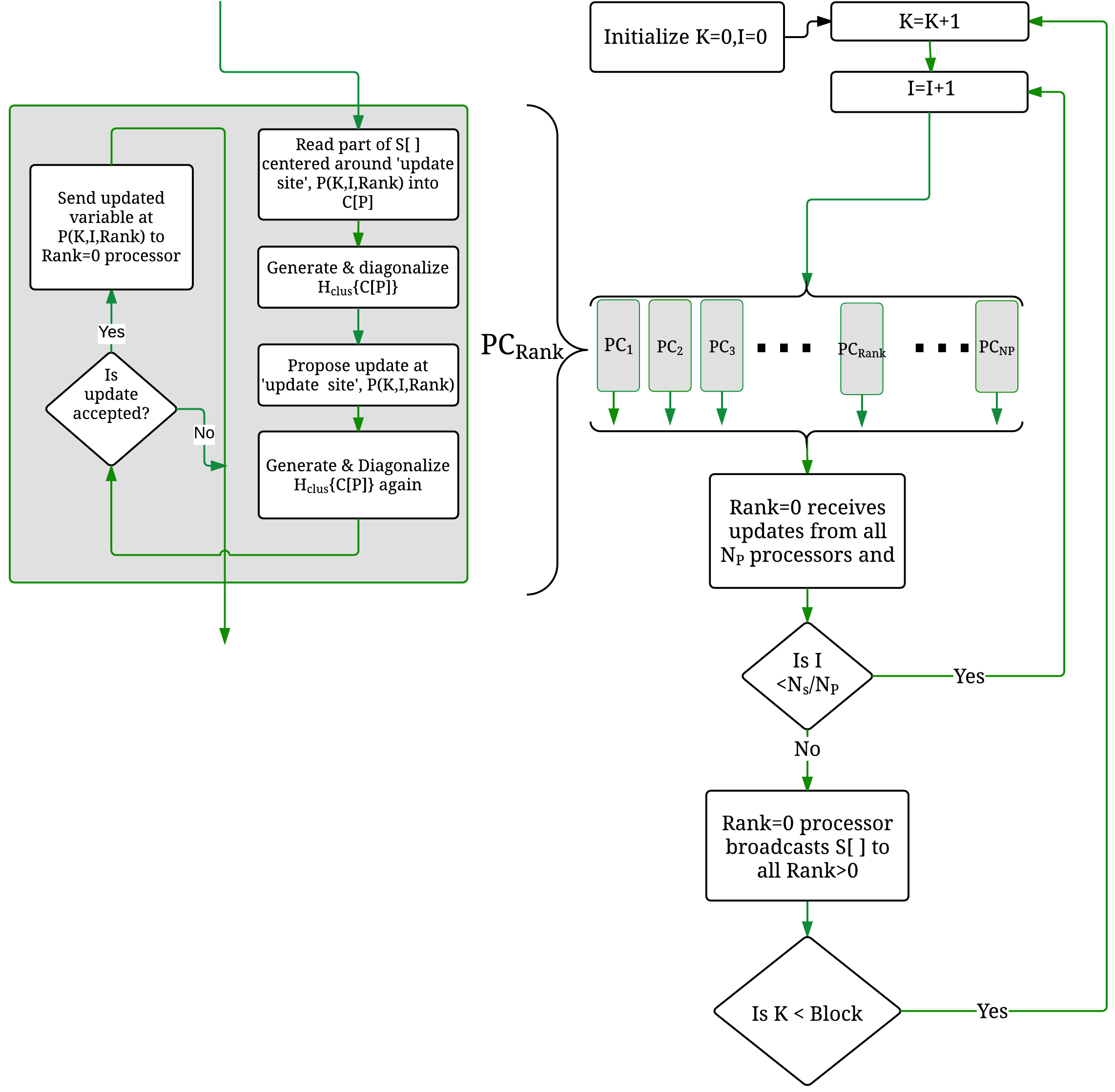
Figure 4: Parallelized TCA flowchart for a single system sweep. Unlike Fig. 2, the loop over the total number of sites of the system is split into two loops: the outer one runs over the number of blocks, while the inner one runs from 1 to the ratio of the number of sites in a block ($N_{S}$) to the number of processors ($N_{P}$). The gray rectangles, labeled $PC_{1}$, $PC_{2}$, …, $PC_{NP}$, are computed on processors with rank 1 through $N_{P}$, respectively. The steps in a typical gray block are displayed on the left. See text for discussion.

We now illustrate that it is possible to further reorganize the TCA algorithm to achieve parallelization. For this we will use Message Passing Interface (MPI) parallelization.

a. PTCA scheme: In Figure 3, a one-dimensional lattice example is used to illustrate the parallelization scheme of TCA. In the figure we show a $N=8$ site system with a $N_{c}=4$ site traveling cluster indicated by a rectangle. The update site is marked in red. Let us start with some initial values for the classical DOF at all the sites. The sites where an update has not yet been proposed are displayed in light blue. The rows from top to bottom indicate the different steps of a single MC system sweep where the update site traverses from left to right sequentially. The sites where the update have been attempted are colored in blue. Here for simplicity of presentation, we discuss the case where the ‘update site’ is the site on the extreme left. Other choice of update sites are discussed in Sec VII. From the figure it is easy to see that assuming the MC system sweep starts from row one, the clusters in the first five rows do not depend on the update of the previous row. Rows six, seven, and eight depend on the outcome of the update attempts at sites one; one and two; and one two and three, respectively. In general, there are $N-N_{c}+1$ clusters of the former kind and $N_{c}-1$ of the later kind. We refer to the later kind as “boundary clusters”.

In TCA the cluster diagonalization involved in all of the eight steps are carried out sequentially. The obvious way to parallelize the TCA is to diagonalize the independent sets of clusters in parallel. The simplest strategy for this is to divide the MC system sweep into two blocks, $L^{\prime}_{1}$ and $L^{\prime}_{2}$, each consisting of four of the eight steps of the MC sweep. It is easy to see that in this way all the four clusters in the block $L^{\prime}_{1}$ can be diagonalized on four processors simultaneously. Once the updated results for $L^{\prime}_{1}$ are received, they are used to generate the clusters for the $L^{\prime}_{2}$ block which can now be diagonalized in parallel. Thus the computation cost is $2N_{c}^{3}$ rather than $NN_{c}^{3}$ as in TCA. For a $d$ dimensional cubic system, the cost of PTCA scales as $2^{d}N_{c}^{3}$. The $2^{d}$ factor comes from the correct accounting of all boundary clusters that can not be diagonalized simultaneously. This still is very advantageous as compared to the $NN_{c}^{3}$ scaling of TCA.

In our approach, the one dimensional global system is broken into two blocks, each having $\frac{N}{2}$ number of sites. In two dimensions, the global square system is broken into four blocks and into eight in three dimensions.

b. PTCA flowchart: We now discuss the implementation of PTCA. The flowchart is presented in Fig. 4 and it is discussed below. For simplicity we discuss specifically the one dimensional case, but a generalization to higher dimensions is straightforward.

For PTCA we will use $N_{P}+1$ processors with ranks 0 to $N_{P}$. As discussed below, of these the rank=0 processor is the master and is involved only in receiving and sending information, while the rest $N_{P}$ processors are the ones that will be used for diagonalization of clusters. As in the TCA case, we define $S[~{}]$ as the array holding all the classical DOF for an $N$ site one dimensional system. As discussed above, we divide the system into two blocks, the loop label running over the blocks is “K”. Within each block, another loop, labeled by “I”, runs from one to $N_{S}/N_{P}$. Here $N_{S}$ is the number of sites within a block and we ensure that $N_{S}/N_{P}$ is an integer. Note that if $N_{S}=N_{P}$ the clusters built at all the $N_{S}$ sites can be diagonalized in one go. In PTCA the “update site”, denoted by $P$, is a function of $N_{S},~{}N_{P}$, and the rank of the processor on which the cluster built around $P$ is to be diagonalized. Thus the update site $P$ is denoted by $P(K,I,Rank)$ in the flowchart. $C[P]$ is the cluster built around the update site $P(K,I,Rank)$. $H_{full}\{S[~{}]\}$ and $H_{clus}\{C[P]\}$ have definitions similar to that for TCA.

The MPI commands used are standard Marc Snir and Dongarra (1998) and will not be repeated here in detail. We use MPI_Init, MPI_Comm_size, MPI_Comm_rank to allocate and assign labels (ranks) to $N_{P}+1$ number of processors. The ranks of the processors range from $0$ to $N_{P}$.

1. Loop over blocks K (= $1,~{}2$) for our one dimensional example.

2. Loop over I goes over $1,2,..,N_{S}/N_{P}$.

3. For each I, assign the construction of the cluster around the “update site” $P(K,I,Rank=R)$ and the subsequent update procedure to the processor with $Rank=R,~{}(R>0$). The $N_{P}$ such assignments are depicted with small gray $N_{P}$ rectangles in Fig. 4.

4. For a processor with $Rank=R,~{}(R>0)$, $C[P]$ will read the relevant $N_{c}$ site classical DOF data from $S[~{}]$. It will then diagonalize $H_{clus}\{C[P]\}$ before and after proposing an update for the classical variable at $P$. If accepted, the update of the $P^{th}$ site is sent to processor with Rank=0 using MPI_SEND. This is shown in the expanded gray rectangle on the left of Fig. 4.

5. Rank=0 processor receives update from all other processors with ranks 1 to $N_{P}$ using MPI_RECV and suitably modifies the $S[~{}]$ on Rank=0 processor.

6. The “I” loop ends.

7. The Rank=0 processor broadcasts the modified $S[~{}]$ to all the processors using MPI_BCAST, once updates from all processors have been received.

8. End the loop K.

The parallelization scheme holds for any dimensions, as long as $N_{c}<N$ which we guarantee by definition. For the simplest case of $N_{S}=N_{P}$, the estimated total cost of $P_{1}$ MC sweeps with $P_{2}$ full system diagonalization for output calculations is $P_{1}2^{d}N_{c}^{3}+P_{2}N^{3}$. This is a huge improvement in performance compared to TCA for which the computational cost for the same would be $P_{1}N\times N_{c}^{3}+P_{2}N^{3}$. The improvement is significant when $P_{1}$ is a very large number, which is always the case. In the next section we present actual results when $N_{S}>N_{P}$ that establishes that even in this case the reduction of numerical cost is significant. For a fixed $P_{1}$ and $P_{2}$, beyond a certain system size, the full system diagonalization will dominate the total computational cost for the PTCA if these are “done on the fly”. We suggest saving configurations and performing the full system diagonalization separately. A strategy for this process using Scalable LAPACK is suggested in section VI.

IV Numerical benchmarks

Let us now discuss benchmarks comparing TCA with PTCA. For this purpose we will use the following spin-fermion Hamiltonian:

$$H_{\rm Hubb-MF} = -t\sum_{\langle i,j\rangle,\sigma}c^{\dagger}_{i,\sigma}c^{\phantom{\dagger}}_{j,\sigma}$$

$$+ \frac{U}{2}\sum_{i}(\langle n_{i}\rangle n_{i}-{\mathbb{m}_{i}}.{\mathbb{\sigma}_{i}})$$

$$+ \frac{U}{4}\sum_{i}({\mathbb{m}_{i}}^{2}-\langle n_{i}\rangle^{2})-\mu\sum_{i}n_{i}.$$

This Hamiltonian is the SU(2) invariant Hartree-Fock mean field Hamiltonian for the Hubbard model. We have recently established Mukherjee et al. (2014) that if the mean field expectation values in $H_{\rm Hubb-MF}$ are treated as classical variables and annealed via a classical MC process involving a slow reduction of the temperature, then the finite temperature results for all the observables we tested agree qualitatively and often quantitatively with Determinant Quantum Monte Carlo. In this model ${\mathbb{m}}_{i}$ is the mean field magnetization at the $i^{th}$ site and it is treated as a classical vector. $t$ is the hopping parameter and $U$ is the Hubbard onsite repulsion. We further set $\langle n_{i}\rangle=1$ for the case of half filling. This model that involves free electrons interacting with the classical spins defines our spin fermion model. We will present results in two and three dimensions and compare with those obtained using ED+MC and TCA in our earlier work Mukherjee et al. (2014). The methods used in [Mukherjee et al., 2014] have also been independently derived and applied in the context of the Hubbard model on an anisotropic triangular lattice Tiwari and Majumdar (2013a) and on geometrically frustrated face centered cubic lattices Tiwari and Majumdar (2013b). Earlier similar approaches but for the attractive Hubbard interaction (negative $U$) where reported in Refs.Mayr et al. (2005); Alvarez et al. (2005); Mayr et al. (2006); Alvarez and Dagotto (2008); Tarat and Majumdar (2014, 2014a, 2014b).

For the results presented in the present paper, the TCA cluster size used is $N_{c}=4^{3}$ in three dimensions and $N_{c}=4^{2}$ in two dimensions. We also checked the independence of our results to variations in the traveling cluster size.

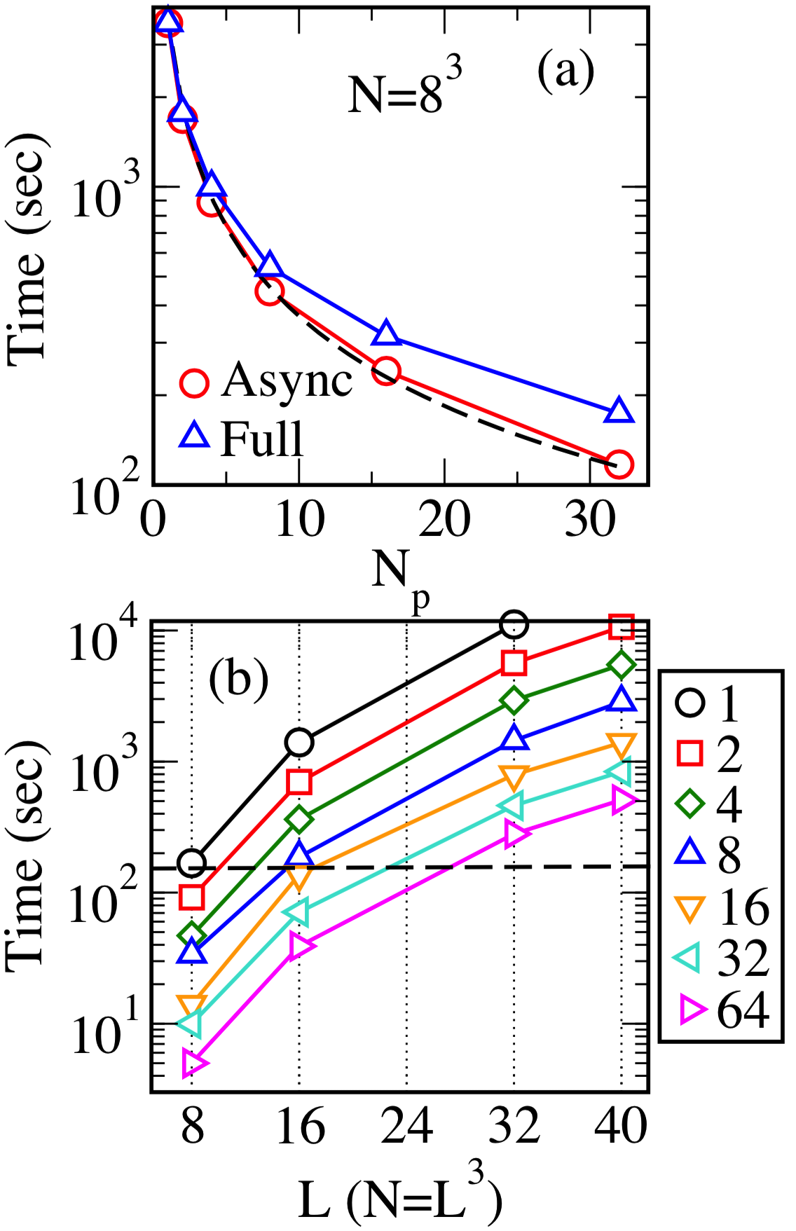
Figure 5: (a) Time required for asynchronous ED and full ED with message passing against the number of processors $N_{P}$ at a fixed $U=8.0t$. See text for definitions. The data is presented for a $N=8^{3}$ lattice using 2000 MC system sweeps at a fixed temperature. The dashed line is the plot of $1/N_{P}$; (b) Time needed for 200 system sweeps for the full calculation with message passing plotted against $L$, for a system size $N=L^{3}$. The data for different number of processors, $N_{P}$, are shown. $N_{P}$ values are indicated on the right. The dashed line indicates that the computational cost for solving a $N=32^{3}$ system using PTCA with 64 processors is almost the same as the time needed using TCA on an $8^{3}$ system with a single processor. Calculations were done using multiple Intel Xeon E5-2670 processors which have eight cores with base frequency of 2.6 Ghz and 8 GB RAM per processor.

For a $L\times L\times L$ system in three dimensions, with a total number of sites $N=L^{3}$, the matrix size of the Hamiltonian for a given configuration of classical fields $\{{\mathbb{m}}\}$ is $2N\times 2N$. The factor of two comes from the two spin species of the fermions. Figure 5 is the main numerical result that establishes (i) the efficiency of PTCA over TCA and (ii) the dependence of the performance of the PTCA on the number of processors $N_{P}$. In (a) we display the bare time, without focusing on measuring physical results, for a $N=8^{3}$ lattice in three dimensions with cubic geometry. We further choose $N_{c}=4^{3}$. We have performed $2000$ MC system sweeps at a fixed temperature, that amounts to $8^{3}\times 2000$ or $1.024\times 10^{6}$ exact diagonalizations of $2\times 4^{3}$ matrices defining the traveling clusters. These are performed using the PTCA approach and employing different numbers of processors. The corresponding time needed is plotted in blue against $N_{P}$. Since large $N_{P}$ increases the communication time between the processors, for comparison in (a) we have also shown the time required to diagonalize the same number of matrices but with no interprocessor communication, labeled as asynchronous. This is indicated in red. Also the curve $1/N_{P}$ (the dashed line) establishes that the time needed for the asynchronous ED varies as $1/N_{P}$ within the PTCA scheme. When the processors communicate (using MPI_SEND, MPI_RECV and MPI_BCAST), the time increases with $N_{P}$. But adds only a few seconds of additional time even for $N_{P}=32$. This is labeled as Full in Fig. 5 (a).

In the previous section we had estimated that the cost of a system sweep in PTCA is $P_{1}2^{d}N_{c}^{3}$, for $P_{1}$ diagonalizations of the traveling cluster. However, this assumed that all independent traveling clusters in one block can be diagonalized simultaneously. Since the system sizes can be very large, this is seldom possible. As a result only a fraction of traveling clusters in one block can be diagonalized simultaneously. It is easy to check that this would lead to the $1/N_{P}$ dependence seen in Fig. 5 (a) apart from the additional processor communication time. In (b) we show the time needed for 200 MC system sweeps within PTCA against $L$, for a $N=L^{3}$ system. This is displayed for different $N_{P}$ values indicated on the right. From (b) it is clear that the time for the 200 system sweeps for a $N=8^{3}$ system with single processor (or within TCA) is almost equal to the PTCA cost for a $32^{3}$ system with $N_{P}=32$.

With this clear advantage of PTCA, in the next section we discuss some particular physics results and compare them with existing literature.

V Results for the Hubbard model in two & three dimensions

In Fig. 6 we discuss the magnetic properties of the Hubbard model in two and three dimensions by studying Hamiltonian Eq. (1) at finite temperature using PTCA. In our recent work we have extensively studied this system using EDMC and TCA Mukherjee et al. (2014). At half filling the Néel temperature, $T_{N}$, has a non monotonic dependence on $U$. These results are presented here in two and three dimensions. In Fig. 6 (a) we plot $T_{N}$ against $U$ for three different system sizes, $4^{3}$, $16^{3}$, and $40^{3}$. These are all obtained using PTCA. The $4^{3}$ results are identical to the $4^{3}$ results in our earlier work. For the larger system sizes studied here we find that $T_{N}$ converges and it has a weak dependence on the finite size of the system. We emphasize that until now in the literature there have been no results for spin-fermion models employing such large number of sites. We use these large system values of $T_{N}$ to perform finite size scaling. In Ref. Mukherjee et al., 2014 we had established that the magnetic structure factor obtained with the TCA agrees with the ED+MC data at all temperatures. This indicates that finite size effects associated with the cluster size do not affect the finite temperature evolution of the magnetic state appreciably. Thus, the finite size scaling using TCA or PTCA is justified.

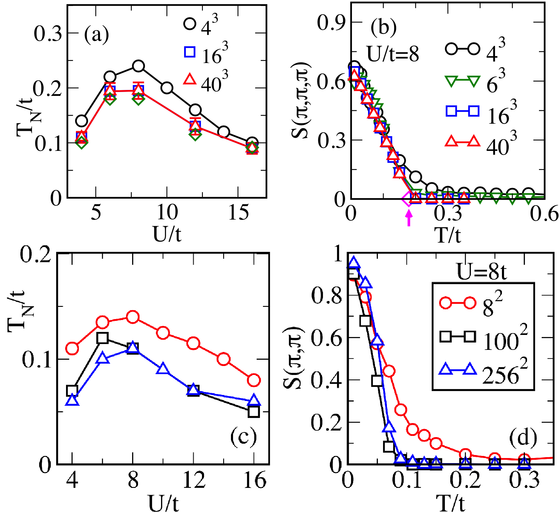
Figure 6: (a) $T_{N}$ vs. $U/t$ for system sizes with $4^{3},16^{3}$, and $40^{3}$ sites. (b) The spin structure factor S($\pi,\pi,\pi$) vs. temperature, for system sizes $4^{3},6^{3},16^{3}$, and $40^{3}$ at $U=8.0t$. The results are obtained using a $4^{3}$ traveling cluster and 16 processors. The data is averaged over 200 configurations obtained from 2000 MC steps for the cases $N=4^{3}$ and $N=6^{3}$, while only 1250 MC steps were used for $N=16^{3}$ and $N=40^{3}$ with an average over 50 configurations. The magenta arrow indicates the thermodynamic $T_{N}$ in this case. (c) and (d) present the corresponding results in two dimensions. (c) $T_{N}$ vs. $U/t$ and (d) the corresponding S($\pi,\pi$)’s for system sizes $8^{2},100^{2}$, and $256^{2}$. The results are obtained using a $4^{2}$ traveling cluster and 16 processors.

For these results on finite systems, the bulk $T_{N}$ estimates are obtained by an inspection of the $S(\pi,\pi,\pi)$ data shown in (b). Information regarding the Néel AFM order is obtained from the magnetic structure factor for the ${\mathbb{m}}$ variables,

$$S({\mathbb{q}})=\frac{1}{N^{2}}\displaystyle\sum\limits_{i,j}e^{i{\mathbb{q}}\cdot({\mathbb{r}}_{i}-{\mathbb{r}}_{j})}\langle{{\mathbb{m}_{i}}\cdot{\mathbb{m}_{j}}}\rangle,$$ (2)

where ${\mathbb{q}}=\{\pi,\pi,\pi\}$ is the wavevector of interest.

Then, assuming that the correlation length $\xi(T_{N}(L)-T_{N}^{Thermo})=aL$ on a $L^{3}$ system, and given that $\xi(x)\propto|x|^{-\nu}$, one arrives at the scaling form, $T_{N}(L)=T_{N}^{Thermo}+bL^{1/\nu}$. Here, $L$ denotes data from a system size $N=L^{3}$. We plot the finite system Néel temperatures against $1/L$ and use $T_{N}^{Thermo}$, $b$, and $\nu$ as fitting parameters. Details of this process are presented in our earlier work, and here in Fig. 6 (a) we simply present the results (green diamonds). We have found that indeed both the $16^{3}$ and $40^{3}$ results converge to the true thermodynamic Néel temperature. For the antiferromagnetic structure factors for different system sizes in (b), we find that the PTCA results for $N>16^{3}$ are virtually identical and appreciably better than the $4^{3}$ and $6^{3}$ results which have non-negligible finite size effects. The arrow in (b) indicates the thermodynamic $T_{N}$ as obtained from finite size scaling for the case $U/t=8$.

In (c) and (d) we show the corresponding results in two dimensions. Here, as it is well known, in principle the Mermin-Wagner theorem establishes that there is no true $T_{N}$ in two dimensions for an $O(3)$ magnet. However, this theorem is valid only for short-range spin-spin interactions. In our case, the integration of the fermions leads to effective spin-spin interactions at all distances, although the rate of the decay of the couplings with distance is unknown. Panels (c) and (d) indicate that the $N=100^{2}$ and $N=256^{2}$ results, while significantly lower than the $8^{2}$ result, are very close to each other suggesting convergence. However, this subtle matter requires further discussion and larger clusters to be fully understood and our goal in this section is merely to check the performance of the proposed PTCA method. The clarification of the validity of the Mermin-Wagner theorem for spin-fermion models is left for the future.

VI Diagonalization of full system

In this section we will discuss the strategy for diagonalizing large full systems to calculate fermionic observables that in principle require all eigenvalues and all eigenvectors for each configuration of classical variables. In the PTCA scheme, given the large matrix sizes for the full system, we find that it is best to first simply anneal the classical variables, then store many equilibrium configurations at each temperature generated during the Monte Carlo process, and then at the end perform full system diagonalizations to calculate the fermionic observables separately. In the special cases where we are interested only in the correlation among classical variables of course we can certainly measure those correlations for each MC configuration. But for the fermionic observable cases that require, e.g., full Green functions we suggest using Scalable LAPACK for the parallel diagonalization of the full system using the equilibrium configurations.

Let us assume $N_{Q}$ are the number of processors used for diagonalizing the large matrices employing Scalable LAPACK. Figure 7 (a) shows the memory required to store all of the arrays that are necessary to diagonalize a large double complex hermitian matrix. It should be noted here that the Hamiltonian as one complete array is never created on an individual processor. Instead, the Hamiltonian is evenly spread out in blocks among all of the processors. This greatly reduces the total RAM required as well as the RAM per processor Blackford et al. (1997). The total RAM and number of processors for a given system is a constant, therefore the ratio of RAM per processor is a fixed quantity. For example, in the traveling cluster used for these calculations, every job (run) submitted is allocated 2 Gb per processor. If one job uses more RAM than this, some processors can not be used since they do not have memory available to them. Therefore, when diagonalizing large matrices using the number of processors that approaches this fixed ratio will optimize the CPU time and memory usage. In (a) we see that, as expected, the memory requirement grows with matrix and system size, but reduces with increasing $N_{Q}$. The $N_{Q}$ values of 4, 8, and 16 are indicated in the figure. The gray region in (a) is where memory needed per processor is 4Gb or less. For typical computational resources of multicore workstations this is easily available. This requirement corresponds to a system size of about $24^{3}$ sites.

The other issue is the time needed for diagonalization. In Fig. 7 (b) we present the typical time needed for single diagonalization corresponding to $N=16^{3}$ and $24^{3}$ system sizes or matrix sizes $8192\times 8192$ and $27648\times 27648$, respectively. The results are for $N_{Q}=4$, $16$, $24$, and $32$ processors. In both cases the time gain is quite significant with increasing $N_{Q}$. If all the configurations over which the output quantities are to be averaged at a fixed temperature are calculated in parallel, then for $N_{Q}=8$ we require only about 0.1 hours of additional computation time for a $N=16^{3}$. For $N=24^{3}$ the additional time is about 2 hours. The additional time goes down further for larger $N_{Q}$. High end workstations and small clusters should easily be able to supply the resources needed for such system sizes.

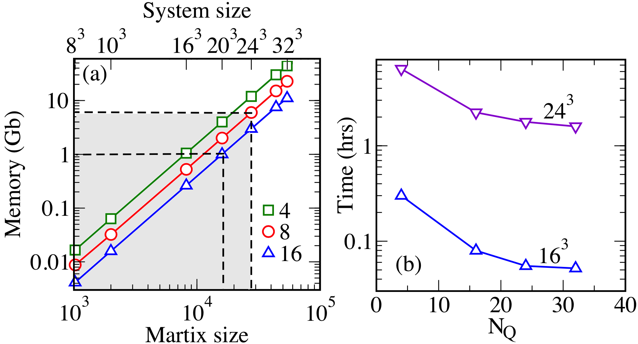
Figure 7: Memory and time needed for a single diagonalization using Scalable LAPACK. In (a) we show the RAM (in Gb) per processor that is required to store the arrays necessary to diagonalize a double complex Hermitian matrix. The gray region is defined by a limit of 4Gb RAM per processor, which can diagonalize a Hamiltonian for a $24^{3}$ system (27648 dimensional matrix) with 8 processors. The data is also presented for 4 and 16 processors; (b) the time needed for a single diagonalization for $16^{3}$ and $24^{3}$ systems vs. the number of processors $N_{Q}$ used in Scalable LAPACK.

VII Discussion

In this section, we will discuss two related numerical issues and provide an estimate for the cost of solving spin-fermion models derived from multiorbital Hubbard models:

a. Cluster size effects: The first is the dependence of results on the traveling cluster size. In Fig. 8 (a) we show the antiferromagnetic structure factor vs. temperature for a lattice with $32^{2}$ sites employing different sizes for the traveling clusters, using the same mean field Hubbard model discussed before.

While small cluster sizes are good enough to capture the long range order as well as the rough location of the transition temperature for this model, the finite cluster sizes introduce finite size effects of its own. To reduce these, one needs to employ larger traveling clusters. In Fig. 8 (a) we see that finite size effects in $T_{N}$ reduce rapidly with larger clusters, $N_{c}=12^{2}$ and $16^{2}$, for the same fixed system size. Furthermore in physical problems where there is long wavelength order, large $N_{c}$ would be crucial to capture the correct phases. In TCA, the linear depencence of the numerical cost on the system size limits $N_{c}$ to $8^{2}$. Larger $N_{c}=12^{2},16^{2}$, results are only possible within the current scheme. We would like to emphasize that this is an additional significant improvement over TCA.

b. Choice of the update site: In Fig. 2 we had displayed a scheme for setting up the PTCA. There we had chosen the leftmost site of the cluster as the site where the update is attempted. Choosing this leftmost “update site” was mainly for convinience. Here we briefly demonstrate the effect of choosing other update sites. The parallelization, of course, applies to any such choice. In Figs. 8 (b) and (c) we show the comparison of results for different choices of the update site. For this purpose, we study the adiabatic Holstein model in one dimension at half filling. The Hamiltonian for this model is

$$H_{\rm Hol} = -t\sum_{\langle i,j\rangle,\sigma}c^{\dagger}_{i,\sigma}c^{\phantom{\dagger}}_{j,\sigma}$$

$$+ \sum_{i}(\lambda x_{i}-\mu)(n_{i}-1)+K/2\sum_{i}x_{i}^{2},$$

where $n_{i}=(n_{i,\uparrow}+n_{i,\downarrow})$. In the particle-hole symmetric adiabatic Holstein model, the classical variables $\{x\}$ at every site denote the static lattice distortions. $\lambda$ is the electron lattice coupling and $K$ regulates the elastic cost of the lattice deformation. In this model the goal is to determine the optimal configuration of the $\{x\}$ variables that minimizes the free energy. At half filling the model exhibits a checkerboard charge order together with large and small lattice distortions Aubry (1995). The charge order can be probed by plotting the structure factor for the classical variables. This is defined by

$$N(q)=\frac{1}{N^{2}}\displaystyle\sum\limits_{i,j}e^{i{q}({r}_{i}-{r}_{j})}\langle{{x_{i}}\cdot{x_{j}}}\rangle,$$ (4)

where $q={\pi}$ is the wavevector of interest.

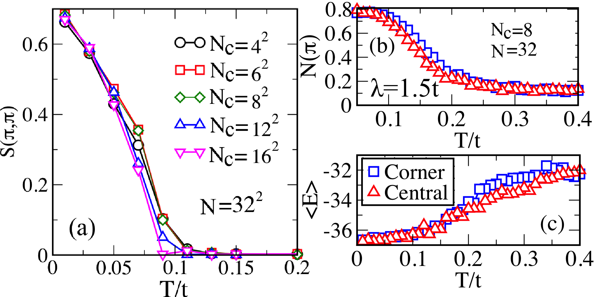
Figure 8: (a) Antiferromagnetic order, S($\pi,\pi$), for the two dimensional Hubbard model at $U/t=8$ using a $N=32^{2}$ lattice with difference traveling cluster sizes as indicated. (b) The one dimensional checkerboard charge order parameter vs. temperature for the adiabatic Holstein model. (c) shows the corresponding average energy of the system with temperature. The data is presented for two schemes indicated as ‘central’ and ‘corner’, see text for discussion. The parameters for (b) and (c) are the same.

In our study two schemes were used: scheme ‘1’ where the update site is the leftmost site of the traveling cluster, and scheme ‘2’ where the $(N_{c}/2+1)^{th}$ site is the update site. In the one dimensional study with $N=32$ and $N_{c}=8$, the sites 1 and 4 are the choices for the update site and the two schemes are refered to as ‘corner’ and ‘central’, respectively. We do not present the details of the algorithm for ‘central’ scheme here, which is very similar to the earlier scheme. We just mention here that one needs to choose a different way of distributing which clusters are to be diagonalized in parallel. The numerical advantage is comparable in both schemes.

In Fig. 8 (b) we study the correlation between the classical variables. $N(q=\pi)$, as defined before, is plotted as a function of temperature. At low temperature an alternating large-small pattern generates a peak at $q=\pi$ in the charge structure factor. As seen in the figure, the results from both schemes match with each other. In addition in (c) we show the average energy with temperature, which also agrees over a wide temperature range.

c. Numerical cost for multiorbital Hubbard model: To derive the general formula for numerical cost of PTCA for a multiorbital Hubbard system, we first note from Sec. IV, that we had divided the system into $2^{d}$ blocks. Thus $N_{S}=N/2^{d}$, where $N_{S}$ is the number of sites in a block. Secondly, since we build a cluster around each of those $N_{S}$ sites in a block, the time taken for a MC system sweep is simply the cost of a single cluster diagonalization times the number of blocks. To do so, however, requires us to diagonalize all $N_{S}$ clusters in a block simultaneously. This would require $N_{S}$ processors. Typically, for large systems, the number of processors $N_{P}$, is much smaller than $N_{S}$. In such cases only $N_{P}$ number of clusters in a block can be diagonalized simultaneously. Thus the cost to complete the diagonalizations of all $N_{S}$ clusters in a block would be $N_{S}/N_{P}$ times the cost of diagonalization of a single cluster.

From these, it is easy to deduce that the cost for $P_{1}$ MC steps in the PTCA as discussed in section IV, $P_{1}2^{d}N_{c}^{3}$, can be written as $P_{1}(N_{c})^{3}\times\frac{N}{N_{P}}$. As a consequence, the cost for $P_{1}$ MC steps for $N_{O}$ orbitals (with two spins per orbital), would be $P_{1}(2N_{O}N_{c})^{3}\times\frac{N}{N_{P}}$. From this expression it can be shown that if $N=N_{P}$ then the cost of PTCA is the cost of $P_{1}$ cluster diagonalizations. If $N_{P}=1$, then the cost grows linearly with $N$, which is precisely the case for TCA. Finally for a general $N_{P}$, the cost scales as $1/N_{P}$.

VIII Conclusions

In conclusion, we have provided a reorganization of the TCA algorithm that allows for a straightforward parallelization. To test the method, we have presented results for the Hubbard model in two and three dimensions treated in the mean field approximation and for the Holstein model with classical lattice distortions in one dimension. A comparison with earlier work clearly shows that the PTCA approach can produce reliable results on very large lattices. Apart from accessing large system sizes for the case of the single orbital Hubbard model, the new approach will facilitate the study of finite temperature effects in multiorbital Hubbard models, treated in the mean field approximation, where the large orbital degeneracy (up to five orbitals in models for iron superconductors) severely limits the number of sites that can be solved employing ED+MC, even when including the TCA improvement.

IX Acknowledgments

We acknowledge the use of the Newton cluster at the University of Tennessee, Knoxville, where all the numerical work was performed. A. M., N.P., and C.B. wrote the computer codes, and gathered and analyzed the results. They were partially supported by the National Science Foundation under Grant No. DMR-1404375. E.D. guided this effort and contributed to the writing of the manuscript. E.D. was supported by the U.S. Department of Energy, Office of Science, Basic Energy Sciences, Materials Science and Engineering Division.

References

- Dagotto (2005) E. Dagotto, Science 309, 257 (2005).
- Tokura and Nagaosa (2000) Y. Tokura and N. Nagaosa, Science 288, 462 (2000).
- Georges et al. (1996) A. Georges, G. Kotliar, W. Krauth, and M. J. Rozenberg, Rev. Mod. Phys. 68, 13 (1996).
- Blankenbecler et al. (1981) R. Blankenbecler, D. J. Scalapino, and R. L. Sugar, Phys. Rev. D 24, 2278 (1981).
- White et al. (1989) S. R. White, D. J. Scalapino, R. L. Sugar, E. Y. Loh, J. E. Gubernatis, and R. T. Scalettar, Phys. Rev. B 40, 506 (1989).
- Paiva et al. (2010) T. Paiva, R. Scalettar, M. Randeria, and N. Trivedi, Phys. Rev. Lett. 104, 066406 (2010), and references therein.
- Schollwöck (2005) U. Schollwöck, Rev. Mod. Phys. 77, 259 (2005).
- Salamon and Jaime (2001) M. B. Salamon and M. Jaime, Rev. Mod. Phys. 73, 583 (2001).
- Tokura (2006) Y. Tokura, Reports on Progress in Physics 69, 797 (2006).
- Serrate et al. (2006) D. Serrate, J. M. D. Teresa, and M. R. Ibarra, Journal of Physics: Condensed Matter 19, 023201 (2006).
- Medarde (1997) M. L. Medarde, Journal of Physics: Condensed Matter 9, 1679 (1997).
- Gou et al. (2011) G. Gou, I. Grinberg, A. M. Rappe, and J. M. Rondinelli, Phys. Rev. B 84, 144101 (2011).
- Dagotto et al. (2001) E. Dagotto, T. Hotta, and A. Moreo, Physics Reports 344, 1 (2001).
- Migdal (1958) A. B. Migdal, Sov. Phys. JETP 7, 996 (1958).
- Kabanov and Mashtakov (1993) V. V. Kabanov and O. Y. Mashtakov, Phys. Rev. B 47, 6060 (1993).
- Born and Oppenheimer (1927) M. Born and R. Oppenheimer, Annalen der Physik 389, 457 (1927).
- Car and Parrinello (1985) R. Car and M. Parrinello, Phys. Rev. Lett. 55, 2471 (1985).
- Yunoki et al. (1998) S. Yunoki, J. Hu, A. L. Malvezzi, A. Moreo, N. Furukawa, and E. Dagotto, Phys. Rev. Lett. 80, 845 (1998).
- Moreo et al. (1999) A. Moreo, S. Yunoki, and E. Dagotto, Science 283, 2034 (1999).
- Kumar and Majumdar (2006a) S. Kumar and P. Majumdar, Phys. Rev. Lett. 96, 016602 (2006a).
- Dong et al. (2008) S. Dong, R. Yu, S. Yunoki, J.-M. Liu, and E. Dagotto, Phys. Rev. B 78, 155121 (2008).
- Dong et al. (2009) S. Dong, R. Yu, J.-M. Liu, and E. Dagotto, Phys. Rev. Lett. 103, 107204 (2009).
- Liang et al. (2011) S. Liang, M. Daghofer, S. Dong, C. Şen, and E. Dagotto, Phys. Rev. B 84, 024408 (2011).
- Şen et al. (2012) C. Şen, S. Liang, and E. Dagotto, Phys. Rev. B 85, 174418 (2012).
- Sanyal and Majumdar (2009) P. Sanyal and P. Majumdar, Phys. Rev. B 80, 054411 (2009).
- Erten et al. (2011) O. Erten, O. N. Meetei, A. Mukherjee, M. Randeria, N. Trivedi, and P. Woodward, Phys. Rev. Lett. 107, 257201 (2011).
- Johnston et al. (2014) S. Johnston, A. Mukherjee, I. Elfimov, M. Berciu, and G. A. Sawatzky, Phys. Rev. Lett. 112, 106404 (2014).
- Park et al. (2012) H. Park, A. J. Millis, and C. A. Marianetti, Phys. Rev. Lett. 109, 156402 (2012).
- Buhler et al. (2000a) C. Buhler, S. Yunoki, and A. Moreo, Phys. Rev. Lett. 84, 2690 (2000a).
- Buhler et al. (2000b) C. Buhler, S. Yunoki, and A. Moreo, Phys. Rev. B 62, R3620 (2000b).
- Moraghebi et al. (2001) M. Moraghebi, C. Buhler, S. Yunoki, and A. Moreo, Phys. Rev. B 63, 214513 (2001).
- Moraghebi et al. (2002a) M. Moraghebi, S. Yunoki, and A. Moreo, Phys. Rev. B 66, 214522 (2002a).
- Moraghebi et al. (2002b) M. Moraghebi, S. Yunoki, and A. Moreo, Phys. Rev. Lett. 88, 187001 (2002b).
- Mayr et al. (2005) M. Mayr, G. Alvarez, C. Şen, and E. Dagotto, Phys. Rev. Lett. 94, 217001 (2005).
- Alvarez et al. (2005) G. Alvarez, M. Mayr, A. Moreo, and E. Dagotto, Phys. Rev. B 71, 014514 (2005).
- Mayr et al. (2006) M. Mayr, G. Alvarez, A. Moreo, and E. Dagotto, Phys. Rev. B 73, 014509 (2006).
- Alvarez and Dagotto (2008) G. Alvarez and E. Dagotto, Phys. Rev. Lett. 101, 177001 (2008).
- Yin et al. (2010) W.-G. Yin, C.-C. Lee, and W. Ku, Phys. Rev. Lett. 105, 107004 (2010).
- Lv et al. (2010) W. Lv, F. Krüger, and P. Phillips, Phys. Rev. B 82, 045125 (2010).
- Dagotto et al. (2011) E. Dagotto, A. Moreo, A. Nicholson, Q. Luo, S. Liang, and X. Zhang, Frontiers of Physics 6, 379 (2011).
- Liang et al. (2013) S. Liang, A. Moreo, and E. Dagotto, Phys. Rev. Lett. 111, 047004 (2013).
- Liang et al. (2012) S. Liang, G. Alvarez, C. Şen, A. Moreo, and E. Dagotto, Phys. Rev. Lett. 109, 047001 (2012).
- Liang et al. (2014) S. Liang, A. Mukherjee, N. D. Patel, C. B. Bishop, E. Dagotto, and A. Moreo, Phys. Rev. B 90, 184507 (2014).
- Raghu et al. (2008) S. Raghu, X.-L. Qi, C.-X. Liu, D. J. Scalapino, and S.-C. Zhang, Phys. Rev. B 77, 220503 (2008).
- Johnston (2010) D. C. Johnston, Adv. Phys. 59, 803 (2010).
- Stewart (2011) G. R. Stewart, Rev. Mod. Phys. 83, 1589 (2011).
- Dai et al. (2012) P. Dai, J. Hu, and E. Dagotto, Nat Phys 8, 709 (2012).
- Dagotto (2013) E. Dagotto, Rev. Mod. Phys. 85, 849 (2013).
- Kumar and Majumdar (2006b) S. Kumar and P. Majumdar, The European Physical Journal B - Condensed Matter and Complex Systems 50, 571 (2006b).
- Kohn (1996) W. Kohn, Phys. Rev. Lett. 76, 3168 (1996).
- Prodan and Kohn (2005) E. Prodan and W. Kohn, Proceedings of the National Academy of Sciences of the United States of America 102, 11635 (2005), http://www.pnas.org/content/102/33/11635.full.pdf+html .
- Kumar and Majumdar (2005) S. Kumar and P. Majumdar, Phys. Rev. Lett. 94, 136601 (2005).
- Marc Snir and Dongarra (1998) S. H.-L. D. W. Marc Snir, Steve Otto and J. Dongarra, MPI: The Complete Reference (The MIT Press, Cambridge, MA, 1998).
- Mukherjee et al. (2014) A. Mukherjee, N. D. Patel, S. Dong, S. Johnston, A. Moreo, and E. Dagotto, Phys. Rev. B 90, 205133 (2014).
- Tiwari and Majumdar (2013a) R. Tiwari and P. Majumdar, arXiv preprint arXiv:1301.5026 (2013a).
- Tiwari and Majumdar (2013b) R. Tiwari and P. Majumdar, arXiv preprint arXiv:1302.2922 (2013b).
- Tarat and Majumdar (2014) S. Tarat and P. Majumdar, EPL (Europhysics Letters) 105, 67002 (2014).
- Tarat and Majumdar (2014a) S. Tarat and P. Majumdar, arXiv preprint arXiv:1402.0817 (2014a).
- Tarat and Majumdar (2014b) S. Tarat and P. Majumdar, arXiv preprint arXiv:1406.5423 (2014b).
- Blackford et al. (1997) L. S. Blackford, J. Choi, A. Cleary, E. D’Azevedo, J. Demmel, I. Dhillon, J. Dongarra, S. Hammarling, G. Henry, A. Petitet, K. Stanley, D. Walker, and R. C. Whaley, ScaLAPACK Users’ Guide (Society for Industrial and Applied Mathematics, Philadelphia, PA, 1997).
- Aubry (1995) S. Aubry, The Hubbard Model (Springer US, 1995).