Calibrating Gyrochronology using Kepler Asteroseismic targets

Abstract

Among the available methods for dating stars, gyrochronology is a powerful one because it requires knowledge of only the star’s mass and rotation period. Gyrochronology relations have previously been calibrated using young clusters, with the Sun providing the only age dependence, and are therefore poorly calibrated at late ages. We used rotation period measurements of 310 Kepler stars with asteroseismic ages, 50 stars from the Hyades and Coma Berenices clusters and 6 field stars (including the Sun) with precise age measurements to calibrate the gyrochronology relation, whilst fully accounting for measurement uncertainties in all observable quantities. We calibrated a relation of the form $P=A^{n}\times(B-V-c)^{b}$, where $P$ is rotation period in days, $A$ is age in Myr, $B$ and $V$ are magnitudes and $a$, $b$ and $n$ are the free parameters of our model. We found $a=0.40^{+0.3}_{-0.05}$, $b=0.31^{+0.05}_{-0.02}$ and $n=0.55^{+0.02}_{-0.09}$. Markov Chain Monte Carlo methods were used to explore the posterior probability distribution functions of the gyrochronology parameters and we carefully checked the effects of leaving out parts of our sample, leading us to find that no single relation beween rotation period, colour and age can adequately describe all the subsets of our data. The Kepler asteroseismic stars, cluster stars and local field stars cannot all be described by the same gyrochronology relation. The Kepler asteroseismic stars may be subject to observational biases, however the clusters show unexpected deviations from the predicted behaviour, providing concerns for the overall reliability of gyrochronology as a dating method.

1 Introduction

1.1 Dating methods for field stars

Many fields of astronomy rely on precise age measurements of Main Sequence (MS) stars. Unfortunately, age is a notoriously difficult quantity to measure for these stars, as observable properties evolve slowly on the MS. Even with high precision spectroscopic measurements, ages often cannot be determined accurately to within 20% (Soderblom, 2010). Some of the most precise age measurements currently available are for stars in clusters where isochrones can be fitted to a coeval population with a range of masses, resulting in age measurements with uncertainties often as low as 10%. Isochronally derived field star ages, on the other hand, are much less precise than this, often having uncertainties of around 50% or more. Demand for age estimates of planet-hosting stars is high, but faint stars observed by Kepler are often expensive or impractical spectroscopic targets. Where high resolution spectra are unavailable, gyrochronology can be extrememly useful. Gyrochronology is a dating method that utilises the potentially predictable rotation period evolution of low mass, MS stars. It requires only knowledge of the current rotation period—which is often easily extracted from Kepler light curves—and mass (or appropriate proxy) of a star. However the current gyrochronology relations are entirely empirically calibrated and still need refining at large stellar ages. Kepler provides the perfect opportunity to calibrate gyrochronology at late ages—it provides surface rotation periods of thousands of stars and new age estimates for hundreds of stars via asteroseismology . This paper aims to use these new asteroseismic age measurements to improve the gyrochronology relations at late ages.

1.2 Gyrochronology

Mass loss via a magnetised stellar wind causes magnetic braking of MS stars (Weber & Davis, 1967). A dynamo-driven magnetic field, generated at the tachocline (the interface between radiative and convective zones) locks the stellar wind to the surface of the star. The stellar wind corotates with the stellar surface out to the Alfvén radius, at which point it decouples and angular momentum is lost from the star. The strength of the magnetic field at the surface, and therefore the rate of angular momentum loss, is related to rotation period (Kawaler, 1988). Due to this dependence, it is postulated that although stellar populations are born with a range of rotation periods, the rapid rotators rapidly lose angular momentum and rotation periods converge onto a well-defined sequence. The timescale for convergence is expected to be around the age of the Hyades for solar mass stars: 650 Myrs (Radick et al., 1987; Irwin & Bouvier, 2009). After this time, rotation periods are thought to be independent of their initial values. Gyrochronology postulates that each star falls on a single three-dimensional plane described by mass, rotation period and age, i.e. given any two of these three properties, one can determine the third. The form of angular momentum evolution described above and calibrated in this article can only be applied to F, G and K MS stars. Fully convective M dwarfs have a different dynamo-driven magnetic field: their rotation periods evolve over extremely long timescales and they often do not converge onto the mass-period-age plane, even after several Gyrs. Hot stars with effective temperatures greater than $\sim$ 6250 K have shallow convective zones—they are almost fully radiative—and, again, they have a different dynamo-driven magnetic field (Kraft, 1967). These massive stars retain their initial rotation period throughout their brief MS lifetimes and are therefore not suitable gyrochronology targets.

The rate of rotation period decay for intermediate mass MS stars was first quantified by Skumanich (1972), who observed that rotation period, lithium abundance and chromospheric activity decay was proportional to the square-root of age. Later, Noyes et al. (1984) added a mass dependence to the period-activity-age relation after more massive stars were observed to spin down more slowly. The term ‘gyrochronology’ was coined by Barnes (2003) who proposed an empirically motivated functional form for the relation between period, colour and age,

$$P=A^{n}\times a(B-V-c)^{b},$$ (1)

where $P$ is rotation period (in days), $A$ is age (in Myr), $B$ and $V$ are B and V band magnitudes respectively and $a$, $b$, $c$ and $n$ are dimensionless free parameters.

This gyrochronology relation was calibrated using open clusters, which are invaluable calibration tools since their ages are known relatively precisely and each cluster contains many stars of the same age which enables the period-mass relation to be tightly constrained. Unfortunately however, the majority of nearby clusters are young and until recently it was difficult to measure rotation periods for all but the youngest, most active stars (using ground–based observations). There is a significant dearth of precisely measured ages for old stars and it is for this reason that the current gyrochronology relations are poorly calibrated at late ages. Barnes (2007) used 8 young open clusters aged between 30 and 650 Myrs to calibrate the dependence of rotation period on mass, and the Sun to calibrate the dependence on age. Best-fit values of $n$, $a$ and $b$ ($c$ was fixed at 0.4) reported in Barnes (2007) are presented in table 1. Equation 1 was further calibrated by Mamajek & Hillenbrand (2008) using updated rotation period and age measurements of stars in open clusters $\alpha$ Per (Prosser et al., 1995), Pleiades (Prosser et al., 1995; Krishnamurthi et al., 1998), M34 (Meibom et al., 2011), and Hyades (Henry, private comm., Radick et al., 1987, 1995; Prosser et al., 1995; Paulson et al., 2004). Once again, the Sun was used as an age anchor—a single data point specifying the shape of the period-age relation. Whereas Barnes (2007) fixed the position of $c$, the ‘colour discontinuity’ in equation 1, at 0.4, Mamajek & Hillenbrand (2008) allow it to be a free parameter in their model. The values of $n$, $a$ and $b$, resulting from their fit are shown in table 1. In both of these studies a maximum likelihood fitting approach was used. This method relies on the assumption that uncertainties are Gaussian, which may not always be the case, and only takes observational uncertainties on the dependent variable into account. As described in §3, we adopt a fitting method that properly accounts for uncertainties on all three observed variables: colour, period and age.

Table 1: Values of a, b, c and n in Barnes (2007) and Mamajek & Hillenbrand (2008) and Angus et al. (2014).

Parameter	Barnes (2007)	Mamajek & Hillenbrand (2008)	Angus et al. (2014)
a	$0.7725\pm 0.011$	$0.407\pm 0.021$	$0.40^{+0.3}_{-0.05}$
b	$0.601\pm 0.024$	$0.325\pm 0.024$	$0.31^{+0.3}_{-0.02}$
c	$0.4$	$0.495\pm 0.010$	$0.45$
n	$0.5189\pm 0.0070$	$0.566\pm 0.008$	$0.55^{+0.02}_{-0.09}$

The data used in this article are described in §2, our calibration and model fitting process is outlined in §3 and the results are presented and discussed in §4.

2 Observations

The ages of 505 Kepler dwarfs and subgiants were published by Chaplin et al. (2014). They made use of two global asteroseismic parameters—the average large frequency separation and the frequency of maximum oscillations power—to estimate stellar properties, including the ages, with a grid-based approach that utilised several different search codes coupled to more than ten grids of stellar evolutionary models.

The ages quoted in Chaplin et al. (2014) come from one of the grid-code combinations, with uncertainties reflecting the scatter between the different sets of results. Chaplin et al. (2014) used two different sets of effective temperatures: one was derived using an Infra-Red Flux Method (IRFM) calibration (Casagrande et al., 2010; Silva Aguirre et al., 2012) and the other from a recalibration of the SDSS griz filter KIC photometry by Pinsonneault et al. (2012) using Yale Rotating Stellar Evolution Code (YREC) models (Demarque et al., 2004). We use the IRFM temperatures since they are less dependent on metallicity, which is not well constrained for the asteroseismic sample, and their uncertainites are more conservative, however our analysis is relatively insensitive to this choice. 87 stars in the asteroseismic catalogue have spectroscopic measurements of $T_{\rm{eff}}$ , and [Fe/H]. These precisely measured spectroscopic properties allowed more tightly constrained ages to be calculated for these 87 stars, which were incorporated where available. In order to produce a relation that predicts the age of a star using only observable properties, we chose to convert $T_{\rm{eff}}$ to $B-V$ for the asteroseismic sample using the relation of Sekiguchi & Fukugita (2000). This conversion added an extra element of systematic uncertainty to our data since the metallicities provided for most of the asteroseismic stars are simply an average value for the field: $-0.2\pm 0.3$ dex (see e.g. Silva Aguirre et al., 2011). However, since the age uncertainties dominate this analysis, we do not expect this to have a significant impact on our results.

The ages quoted in Chaplin et al. (2014) have typical uncertainties of 35%. These large uncertainties are the result of the fact that only approximate inferences can be made on the ages using the global asteroseismic parameters, neither of which has an explicit dependence on age. It will be possible, however, to derive more precise ages for a subset of these stars. By measuring the frequency of each oscillation mode individually, not just the global asteroseismic parameters, one can provide much tighter constraints on ages. Ages derived from individual oscillation mode measurements can have uncertainties as small as 10% (Brown & Gilliland, 1994; Silva Aguirre et al., 2013). However, measuring frequencies for individual oscillation modes is a manual process and can only be applied in the highest signal-to-noise cases. Chaplin et al. (2014) predict that around 150 of the 505 stars will be suitable for this individual oscillation mode treatment. We obtained precise ages for 42 stars from Metcalfe et al. (2014), modelled with the Asteroseismic Modeling Portal (AMP), with effective temperatures and metallicities from Bruntt et al. (2012). Of the 42 stars in Metcalfe et al. (2014), we only incorporate the ‘simple stars’ (cool dwarfs) into our sample, ignoring the hotter F stars and more evolved subgiant stars as these are not expected to follow the simple gyrochronology relation.

The Kepler light curves of the 505 asteroseismic targets display quasi-periodic variations on timescales corresponding to the rotational periods of the stars—flux variations are produced by active regions on the stellar surface that rotate in and out of view. Rotation periods for 310 of these stars are published in Garcia et al. (2014) who used a combination of an autocorrelation function and wavelet transform method to measure surface rotation. From the 505 targets in the original sample, 310 rotation periods were reliably measured, 14 of which have precise asteroseismic ages from AMP modelling. All stars in the asteroseismic sample with rotation periods published by McQuillan et al. (2014), also appear in the rotation period catalogue of Garcia et al. (2014). There is excellent agreement between rotation period measurements where the two catalogues overlap. Of the 114 stars which appear in both catalogues, only the rotation periods of 4 were not consistent at the 1$\sigma$ level and of these only 1, KIC 4931390, was inconsistent at greater than 2$\sigma$. The similarities between the two catalogues is further described in Garcia et al. (2014).

The asteroseismic sample covers a large range of ages, however it does not provide good mass coverage across the entire range (see figures 1 and 2). Few stars have temperatures below 6000 K ($B-V$ $\sim$ 0.55) and of the low mass stars, most of them are old (note that massive stars evolve rapidly and so we do not expect many in the sample). The exclusion of young, low-mass stars from the asteroseismic sample is due to the fact that these stars are more active and their power-spectra do not display high signal-to-noise acoustic oscillations. The omission of these as well as other types of stars that are not ideal asteroseismic targets from our sample should not bias our results. The mere lack of data in some regions of parameter space will not skew the best fitting model, however it is important to note that the resulting gyrochronology relation will not necessarily be descriptive of those stars not represented in this sample. We filled in some of the missing parameter space by adding 50 stars to our sample from young clusters Coma Berenices (0.5 Gyr), and the Hyades (0.625 Gyr) (see table 2). Clusters younger than 0.5 Gyr often have large populations of rapid rotators that have not yet converged onto the gyrochronology plane, so no clusters younger than Coma Ber were included. Uncertainties on $B-V$ colours associated with each cluster star were not provided in the catalogues from which rotation periods and ages were obtained. Since the uncertainty associated with each measurement plays such a key role in our analysis (see §3), we assigned an uncertainty of $\pm 0.01$ mag to each colour measurement, based on a realistic estimate of the typical uncertainties expected. The 1.1 and 0.588 Gyr open clusters, NGC 6811 and Praesepe, were originally included in our analysis. However we discovered that their period-colour relations were different to those of the Hyades and Coma Ber, as well as to each other’s, and we therefore did not include them in our final analysis. A further 6 field stars with precise age measurements were added to the sample: 16 Cyg A and B, Alpha Cen A and B, 18 Sco and, of course, the Sun (see table 3). The entire set of 365 stars is shown in figures 1 and 2. Asteroseismic targets are shown in grey, with cluster and field stars in blue and the Sun in red.

Figure 1: Photometric rotation period vs age for 310  Kepler targets (grey circles) plus cluster and field stars (blue triangles). The Sun is shown as a red circle.

Figure 2: Photometric rotation period vs $B-V$ colour for the data described in figure 1.

Table 2: Clusters and References: (1) Dobbie et al. (2009), (2) Collier Cameron et al. (2009), (3) Perryman et al. (1998), (4) Radick et al. (1987).

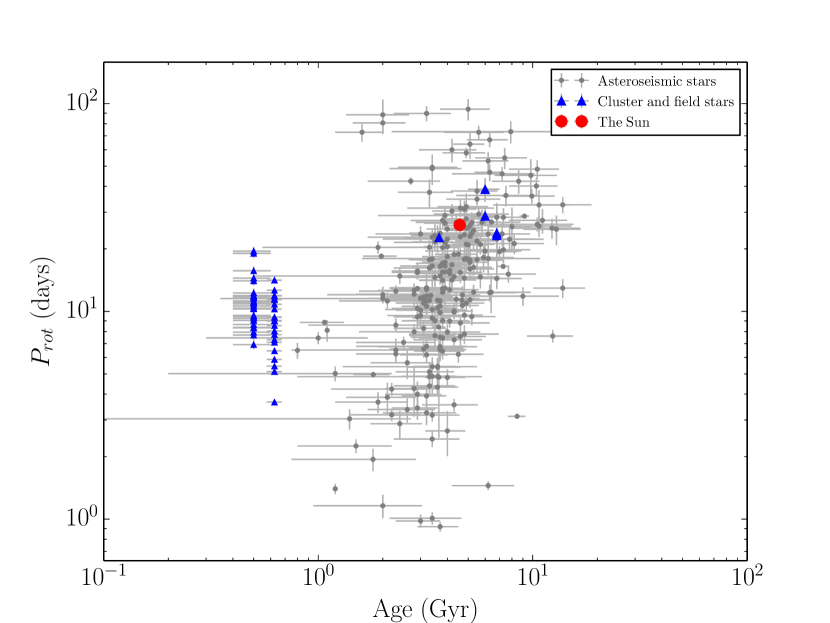
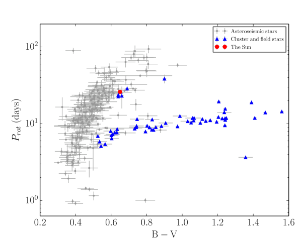
Cluster	Age (Gyr)	Number of stars	Age ref	Rotation period ref
Coma Ber	0.5 $\pm$ 0.1	28	1	2
Hyades	0.625 $\pm$ 0.05	22	3	4

Table 3: Rotation periods and $B-V$ colours for field stars with precise ages. Notes: Davies et al. (2014) measured internal rotation periods for 16 Cyg A and B using asteroseismology. However, this is likely to be close to the surface rotation value. Rotation periods for and $\alpha$ Cen A and B were measured from variation in chromospheric emission lines. High-resolution spectropolarimetric observations were used to measure a rotation period for 18 Sco. The age of 16 Cyg AB was measured with asteroseismology. 18 Sco’s age measurement was based chiefly on an asteroseismic analysis, however its rotation period was used as an additional constraint, so the age estimate is not entirely independent of rotation period for this star. An age for the $\alpha$ Cen system was estimated from spectroscopic observations with additional seismic constraints.

ID	age	$P_{rot}~{}$	$B-V$	References
16 Cyg A	6.8 $\pm$ 0.4	23.8 ${}^{+1.5}_{-1.8}$	0.66 $\pm$ 0.01	Metcalfe et al. (2012), Davies et al. (2014), Moffett & Barnes (1979)
16 Cyg B	6.8 $\pm$ 0.4	23.2 ${}^{+11.5}_{-3.2}$	0.66 $\pm$ 0.01	Metcalfe et al. (2012), Davies et al. (2014), Moffett & Barnes (1979)
18 Sco	3.7 $\pm$ 0.2	22.7 $\pm$ 0.5	0.64 $\pm$ 0.01	Li et al. (2012), Petit et al. (2008), Mermilliod (1986)
The Sun	4.568 $\pm$ 0.001	26.09 $\pm$ 0.1	0.65 $\pm$ 0.001	Bouvier & Wadhwa (2010), Donahue et al. (1996), Cox & Pilachowski (2000)
$\alpha$ Cen A	6 $\pm$ 1	28.8 $\pm$ 2.5	0.69 $\pm$ 0.01	Bazot et al. (2012), Yıldız (2007), Hallam et al. (1991), Mermilliod (1986)
$\alpha$ Cen B	6 $\pm$ 1	38.7 $\pm$ 5.0	0.90 $\pm$ 0.01	Bazot et al. (2012), Yıldız (2007), Dumusque et al. (2012), Mermilliod (1986)

3 Calibrating the Gyrochronology relation

3.1 The model

The 310 asteroseismic stars in our sample have $B-V$ colours converted from effective temperatures, photometric rotation periods, asteroseismic ages, and asteroseismic surface gravities. Each measurement of these properties is assumed to be independent with an associated Gaussian uncertainty. Not all of the cluster stars added to our sample have log g values; however, since we only use log g to separate the populations of subgiants and dwarfs (and we assume that the cluster stars are dwarfs) this should not affect our results. Following the treatment of Barnes (2007) and Mamajek & Hillenbrand (2008), rotation period was treated as the dependent variable throughout the modelling process.

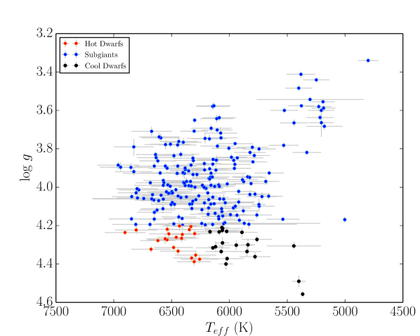
Hot stars and subgiants follow a different gyrochronology relation to MS dwarfs. Stars with effective temperatures above the Kraft-break, $T_{\rm{eff}}\sim$ 6250 K, (Kraft, 1967) do not have a thick convective envelope and cannot support a strong magnetic dynamo, so do not spin down appreciably during their MS lifetimes. Subgiants spin down rapidly as they expand due to angular momentum conservation and thus diverge from the gyrochronological mass-period-age plane. The point in their evolution at which they depart, the ‘gyrochronological MS turn off’, is difficult to define. Classically, MS turnoff is defined as the hottest point on a star’s path on the HR diagram (before it ascends the giant branch) but theory predicts that evolving stars begin the process of spinning down relatively slowly after leaving the classically defined MS (van Saders & Pinsonneault, 2013). For this reason we chose a very simple definition of MS turnoff: we defined a log g boundary of 4.2 to mark the transition between dwarfs and giants. We tried a range of boundary values and found that 4.2 minimised subgiant contamination whilst maximising the cool dwarf sample. It was also necessary to use a mixture model to account for misclassified subgiants—without it, subgiant contamination significantly biased the resulting fit. We did not exclude hot stars and subgiants from our sample during the modelling process, we modelled all three populations simultaneously. This allowed for the fact that stars have some probability mass lying in all three regimes due to their large observational uncertainties.

Hot MS stars were defined as those with $B-V$ $<$ 0.45, corresponding to $T_{\rm{eff}}$$~{}\approx$ 6250 K for solar metallicity and log g. Since there is no dependence of rotation period on age for massive MS stars, their rotation periods were modelled as a normal distribution with mean and standard deviation, $Y$ and $V$, as free parameters. Subgiant rotation periods do depend on age and $T_{\rm{eff}}$. However, since the rotational properties of these stars are not interesting for the purposes of gyrochronology calibration, we also modelled them with a normal distribution with mean and standard deviation, $Z$ and $U$, as free parameters. We used a mixture model for the remaining population of stars, consisting of cool dwarfs and misclassified, contaminating subgiants. The subgiants were treated as if their rotation periods had been drawn from a background normal distribution with mean and standard deviation, $X$ and $U$, again inferred from the data and another parameter, $Q$, the probability of each star belonging to that background population. The results of this analysis were not particularly sensitive to the choice of distribution for the hot stars and subgiants. These models were put in place so that we did not have to throw any data away and we could model everything at once. This was important because stars were classified according to their observed temperatures and log gs, which are noisy. Due to the large uncertainties on $T_{\rm{eff}}$ and log g, each star therefore has some probability of being a subgiant, some of being a cool dwarf and some of being a hot star. By throwing away data, one could accidentally throw away a misclassified star. We avoid this problem by modelling all stars simultaneously and taking a probabilistic approach to classification. Inferences made about the parameters of the normal distributions used to model subgiants and hot stars were not of particular interest for the purposes of gyrochronology calibration. We decided to use simple normal distributions rather than more physically motivated models in order to remain as model–independent as possible. Figure 3 shows log g vs $T_{\rm{eff}}$ for the asteroseismic stars. Stars classified as cool dwarfs are shown in black, hot dwarfs in red and subgiants in blue.

Figure 3: log g vs $T_{\rm{eff}}$ for the 310 asteroseismic stars. Hot dwarfs with $T_{\rm{eff}}$$~{}>$ 6250 K and log g$~{}>$ 4.2 are red, subgiants with log g$~{}<$ 4.2 are blue. Only the black cool dwarfs with $T_{\rm{eff}}$$~{}<$ 6250 K and log g$~{}<$ 4.2 are expected to follow the gyrochronology relation in equation 1.

Ideally both the hot star ($B-V$ $<$ 0.45) and subgiant (log g$<$ 4.2 ) boundaries would be free parameters in our model. However, since these two populations were modelled with a relatively unconstraining normal distributions, these boundary parameters would not be well behaved. Both would be pushed to higher and higher values until all stars were modelled with a normal distribution. In order to avoid this problem, we fixed these two boundaries. A future analysis could avoid the assumption that the gyrochronology relation is infinitely narrow and assign it some intrinsic width, which would also be a free parameter.

We postulate that there is a deterministic relationship between the ‘true’ rotation period of a cool MS star and its ‘true’ age and colour, described by equation 1 (by ‘true’ we mean the value an observable property would take, given extremely high signal-to-noise measurements). Rotation period also depends on log g since this property determines whether a star falls in the dwarf or subgiant regime.

In what follows we use $P$ to denote rotation period and define $\mathbf{w}=(age,B-V,~{}\log~{}g)$ as the vector of additional observational properties. Observations are denoted as $\hat{P}_{n}$ and $\hat{\mathbf{w}}_{n}$ and the unobserved (latent), ‘true’ parameters as $P_{n}$ and $\mathbf{w}_{n}$ for stars $1,...,N$.

In order to explore the posterior Probability Distribution Functions (PDFs) of the model parameters, $\theta$, conditioned on a set of noisy observations, $\{\hat{P}_{n},\hat{\mathbf{w}}_{n}\}$, it was necessary to marginalise over the latent parameters, $\{P_{n},\mathbf{w}_{n}\}$. This is because the model parameters, $\theta$ are conditionally dependent on the ‘true’ values of rotation period and colour, not the observed values themselves. The observed values are only conditionally dependent on the ‘true’ values. In order therefore to infer the values of the model parameters using the observed values of rotation period and colour, it was necessary to marginalise over the latent parameters. Assuming all measurements are independent, the marginalised likelihood can be written

$$p(\{\hat{P}_{n},\hat{\mathbf{w}}_{n}\}|\theta)=\prod_{n=1}^{N}\int p(\hat{P}_{n},\hat{\mathbf{w}}_{n},P_{n},\mathbf{w}_{n}|\theta){\rm d}P_{n}{\rm d}\mathbf{w}_{n}.$$ (2)

The joint probability, on the right hand side of this equation, can be factorised as

$$p(\hat{P}_{n},\hat{\mathbf{w}}_{n},P_{n},\mathbf{w}_{n}|\theta)=$$ (3)

$$p(P_{n}\,| \,\mathbf{w}_{n},\theta)p(\hat{P}_{n}\,|\,P_{n})\,p(\hat{\mathbf{w}}_{n}\,|\,\mathbf{w}_{n})p(\mathbf{w}_{n}),$$

where we have utilised the fact that the observations, $\hat{P}_{n}$ and $\hat{\mathbf{w}}_{n}$ are conditionally independent of the model parameters, $\theta$: they only depend on $\theta$ through the latent parameters, $P_{n}$ and $\mathbf{w}_{n}$. The above integral can be written

$$p(\{\hat{P}_{n},\hat{\mathbf{w}}_{n}\}|\theta)\propto \prod_{n=1}^{N}\int p(\mathbf{w}_{n}|\hat{\mathbf{w}}_{n}){\rm d}\mathbf{w}_{n}$$

$$\int p(P_{n}|\mathbf{w}_{n},\theta)p(\hat{P}_{n}\,|\,P_{n}){\rm d}P_{n},$$

where we have used Bayes’ theorem: $p(\mathbf{w}_{n}|\hat{\mathbf{w}}_{n})\propto p(\hat{\mathbf{w}}_{n}|\mathbf{w}_{n})p(\mathbf{w}_{n})$. The outer integral is the same for hot dwarfs, cool dwarfs and subgiants alike. In our model, the probability of the ‘true’ rotation period given the ‘true’ observed parameters and the model parameters, $p(P_{n}|\mathbf{w}_{n},\theta)$, is different in each regime because a different generative process is responsible for producing rotation periods. For cool dwarfs ($B-V$ $<$ 0.45 and log g$~{}>$ 4.2 ):

$$p(P_{n}|\mathbf{w}_{n},\theta) = (1-Q)~{}\delta\left(P_{n}-f_{\theta}(\mathbf{w}_{n})\right)$$

$$+\quad Q\,\left(\sqrt{2\pi U^{2}}\right)^{-1/2}$$

$$~{}\exp\left({-\frac{(P_{n}-X)^{2}}{2U^{2}}}\right),$$

where $Q$ is the probability that a star is drawn from the population of misclassified subgiants and

$$f_{\theta}(\mathbf{w}_{n})=A^{n}\times a(B-V-c)^{b}$$ (6)

is the gyrochronology relation. For hot dwarfs ($B-V$ $<$ 0.45 and log g$~{}>$ 4.2 ) the generative process is:

$$p(P_{n}\,|\,\mathbf{w}_{n},\theta)=\left(\sqrt{2\pi V^{2}}\right)^{-1/2}~{}\exp\left({-\frac{(P_{n}-Y)^{2}}{2V^{2}}}\right),$$ (7)

and for subgiants,

$$p(P_{n}\,|\,\mathbf{w}_{n},\theta)=\left(\sqrt{2\pi W^{2}}\right)^{-1/2}~{}\exp\left({-\frac{(P_{n}-Z)^{2}}{2W^{2}}}\right).$$ (8)

We used hierarchical inference to account for observational uncertainties, following the method of Hogg et al. (2010), also used by Foreman-Mackey et al. (2014), Rogers (2014), Morton & Winn (2014) and Demory (2014). We computed equation 3.1 up to an unimportant constant using a sampling approximation. The values of $\hat{P}_{n}$ and $\hat{\mathbf{w}}_{n}$ with uncertainties, $\sigma_{P}$ and $\sigma_{\mathbf{w}}$, reported in catalogues provide constraints on the posterior probability of those variables, under a choice of prior PDF, $p_{0}(\hat{\mathbf{w}}_{n})$. Ideally, these catalogues would provide posterior PDF samples, not just point estimates, which we could use directly. i.e. samples from

$$p(\mathbf{w}_{n}|\hat{\mathbf{D}}_{n})=\frac{p(\hat{\mathbf{D}}_{n}|\mathbf{w}_{n})p_{0}(\mathbf{w}_{n})}{p_{0}(\hat{\mathbf{D}}_{n})},$$ (9)

where $p(\hat{\mathbf{D}}_{n}|\mathbf{w}_{n})$ is the likelihood of the data, $\hat{\mathbf{D}}_{n}$ (in this case, the set of Kepler lightcurves plus spectroscopic $T_{\rm{eff}}$ and [Fe/H] measurements), given the model parameters, $\mathbf{w}_{n}$. $p_{0}(\hat{\mathbf{w}}_{n})$ is an uninformative prior probability distribution function $p_{0}(\mathbf{w}_{n})$ is an uninformative prior PDF, chosen by the fitter (Chaplin et al., 2014, used a flat prior PDF in age and log g). In the absence of posterior PDF samples we generated our own from Gaussian distributions with means, $\hat{\mathbf{w}}_{n}$ and standard deviations, $\sigma_{\mathbf{w}}$. $J$ posterior samples were generated for each star (we used $J$ = 500):

$$\mathbf{w}_{n}^{(j)}\sim p(\mathbf{w}_{n}\,|\,\hat{\mathbf{w}}_{n}),$$ (10)

and were used to evaluate $p(\mathbf{w}_{n}|\hat{\mathbf{w}}_{n})$ up to a normalisation constant. Using these samples we computed the marginalised likelihood for a single star as follows,

$$p(\hat{P}_{n},\hat{\mathbf{w}_{n}}\,|\,\theta)\approx\frac{1}{J_{n}}\sum_{j=1}^{J_{n}}p(\hat{P}_{n}\,|\,\mathbf{w}_{n}^{(j)},\theta)\quad.$$ (11)

The argument inside this sum is given by the integral

$$p(\hat{P}_{n}\,|\,\mathbf{w}_{n}^{(j)},\theta)=\int p(P_{n}|\mathbf{w}_{n},\theta)p(\hat{P}_{n}\,|\,P_{n}){\rm d}P_{n}\quad.$$ (12)

Assuming that the period uncertainties are Gaussian with mean $\hat{P}_{n}$ and variance ${\sigma_{n}}^{2}$, this integral can be evaluated analytically for each population. For example, starting from equation 3.1 the result for the cool dwarfs is

$$p(\hat{P}_{n}\,|\,\mathbf{w}_{n}^{(j)},\theta) = \frac{1-Q}{\sqrt{2\,\pi\,{\sigma_{n}}^{2}}}\exp\left(-\frac{\left[\hat{P_{n}}-f_{\theta}(\mathbf{w}_{n}^{(j)})\right]^{2}}{2\,{\sigma_{n}}^{2}}\right)$$ (13)

$$+\frac{Q}{\sqrt{2\,\pi\,(U^{2}+{\sigma_{n}}^{2})}}\exp\left(-\frac{[\hat{P_{n}}-X]^{2}}{2\,[U^{2}+{\sigma_{n}}^{2}]}\right)\quad.$$

A similar result can be derived for the other populations.

Finally, using these analytic results for the inner integral, the marginalised log-likelihood from equation 3.1 becomes

$$\log p(\{\hat{P}_{n},\hat{\mathbf{w}}_{n}\}\,|\,\theta)\approx$$

$$\log\mathcal{Z}+\sum_{n=1}^{N}\log\left[\sum_{j=1}^{J_{n}}p(\hat{P}_{n}\,|\,\mathbf{w}_{n}^{(j)},\theta)\right]$$

where $\mathcal{Z}$ is an irrelevant normalisation constant. We used emcee (Foreman-Mackey et al., 2013), an affine invariant, ensemble sampler Markov Chain Monte Carlo (MCMC) algorithm, to explore the posterior PDFs of the model parameters, $\theta$. Flat prior PDFs were used for each parameter. Following the above method, a likelihood was computed as follows:

• For each star, $J$ samples were drawn from three normal distributions: one in colour, one in age and one in log g, where the means and standard deviations of those distributions were the observed values and uncertainties. This step was performed just once and the following steps were performed for each likelihood evaluation.

• For those samples that fell in the cool dwarf regime ($B-V$ $>$ 0.45 and log g$~{}>$ 4.2 ), model rotation periods were both calculated using equation 1 and assigned the value of parameter $X$. A Likelihood for the two model rotation periods were then evaluated using a Gaussian mixture model likelihood function.

• For the samples that fell in the hot dwarf ($B-V$ $<$ 0.45 and log g$~{}>$ 4.2 ) and subgiant (log g$~{}<$ 4.2 ) regimes, likelihoods were calculated by comparing observed rotation periods with the model rotation periods for the two populations: $Y$ and $Z$.

• The total log-likelihood for each star was calculated as the sum of the log-likelihoods of each of the $J$ samples.

• Finally, the sum of individual star log-likelihoods provided the total log-likelihood.

4 Results and Discussion

Table 4: Median values of $a$, $b$, $c$ and $n$ for individual clusters (see equation 1).

Parameter	Coma Berenices	Hyades
a	$0.417^{+0.08}_{-0.07}$	$0.312^{+0.04}_{-0.06}$
b	$0.271^{+0.05}_{-0.06}$	$0.410^{+0.05}_{-0.04}$
n	$0.542\pm 0.03$	$0.599^{+0.03}_{-0.02}$

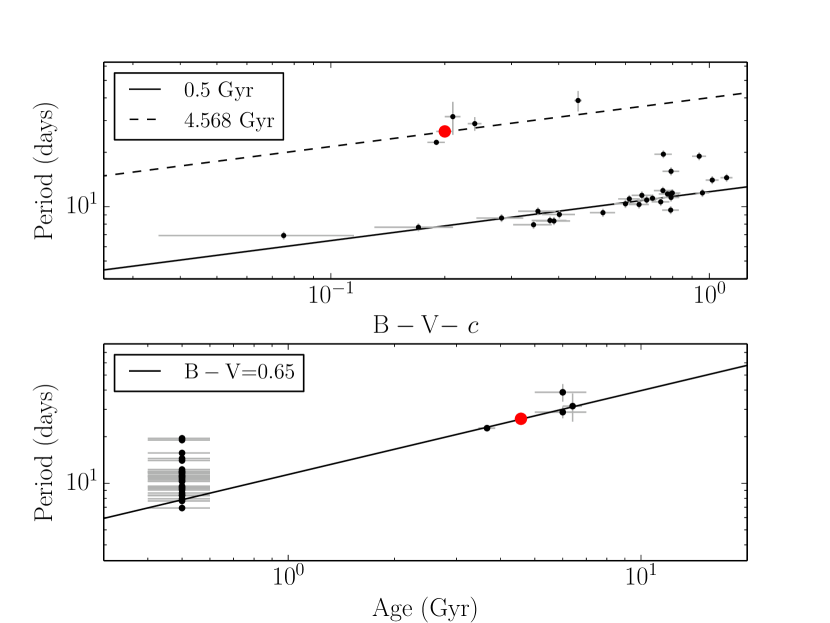
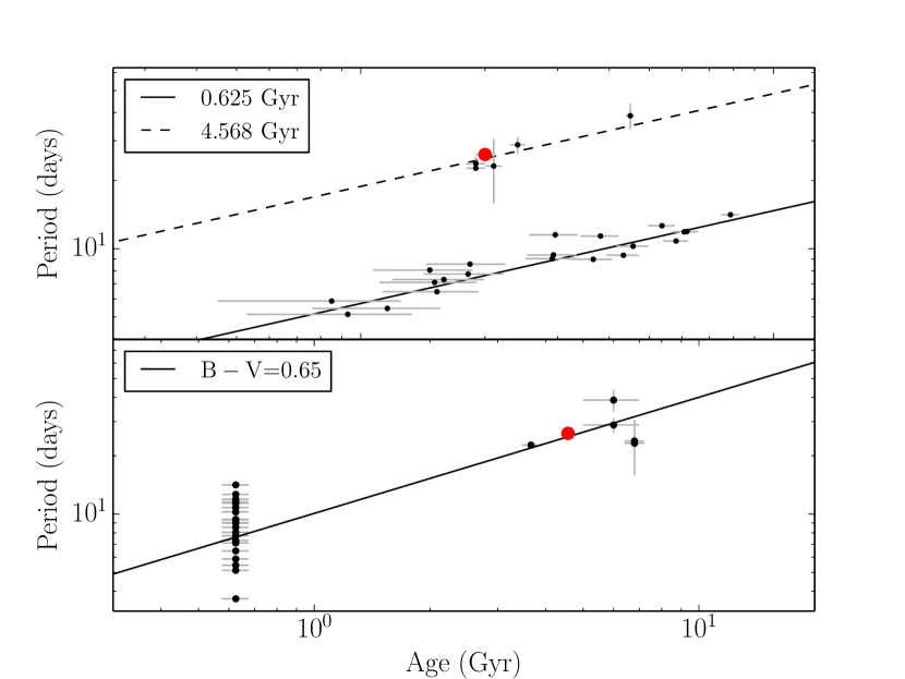
A gyrochronology relation was initially fit to the asteroseismic stars, the field stars and four clusters (Hyades, Coma Berenices, Praesepe and NGC 6811) all together. However, this resulted in extremely multi-modal posteriors PDFs for $a$, $b$ and $n$. After fitting a separate relation to various subsets of the data, it became evident that a lower value of $b$ was preferred by NGC 6811, i.e. the slope of the $\log(\mathrm{period})-\log(B-V-c)$ relation was shallower for NGC 6811 than for the Hyades, Coma Berenices and Praesepe. We therefore exluded NGC 6811 from our sample and attempted to fit a relation to the remaining data. Multi-modal posterior PDFs were still produced however, until Praesepe was also removed from the sample. The reason for this multi-modality is unclear, however we tentatively attribute it to Praesepe preffering a different value for the colour discontinuity, $c$, to the Hyades and Coma Berenices. We calculated the likelihood for Praesepe, plus the field stars (to provide the age dependence) with two different values of $c$: $0.45$ and $0.5$, finding a higher likelihood for $c=0.5$. Since we do not fully understand the cause of this variation in $c$, and in order to keep our model simple, we chose to also exclude Praesepe from our final data set and fit a gyrochronology relation with $c=0.45$ to the remaining data (asteroseismic stars, field stars, Hyades and Coma Berenices). We also fitted relations with $c$ values ranging from 0.4 to 0.55 to this final data set, finding that the results were relatively insensitive to variations in this parameter (solar ages predicted from each best-fitting model were consistent within uncertainties). Individual fits to Hyades and Coma Berenices, plus the field stars are shown in figures 4(a) and 4(b). Median values of $a$, $b$ and $n$ for the two clusters with their 16th and 84th percentile uncertainties are provided in table 4. Note that none of these parameters are fully consistent between the two clusters. The fact that each cluster seems to prefer a different value of $a$, $b$, $n$ and $c$ paints a concerning picture for this form of a gyrochronology relation which assumes one set of parameters can be used to describe all stars. It is likely that the inability of equation 1 to fully describe the observed properties of our sample of stars is due to the simplifying assumptions that go into this relationship. The fact that there is no dependence on metallicity, for example, may contribute to the deficiencies of this model. One might expect metallicity to have an effect on the rotational evolution of a star since it impacts its internal structure. We have not attempted to calibrate a metallicity-dependent gyrochronology relation, because there are no precise metallicity measurements for the majority of the Kepler stars, on which this study is chiefly based. In addition, we anticipate that the majority of stars for which this new gyrochronology relation will be most useful are Kepler stars, or stars targeted by missions like Kepler, again, the majority of which are unlikely to have precise metallicities.

(a) Rotation period vs $B-V-c$ for the Hyades (top) and Coma Berenices (bottom).

(b) Rotation period vs age for the Hyades (top) and Coma Berenices (bottom).

Figure 4: Individual fits to the clusters and field stars. The Sun is the red point. The top figure shows rotation period vs ‘$B-V-c$’ for the Hyades (top) and Coma Berenices (bottom) with Solar and cluster age isochrones. The bottom figure shows rotation period vs age for the Hyades (top) and Coma Berenices (bottom) with the period- age relation for a constant $B-V$ value of 0.65 (Solar $B-V$).

Table 5: Median values of the parameters describing the populations of non-gyrochronological stars.

Parameter	Median value
$U$	8${}^{+4}_{-2}$ days
$V$	2.1${}^{+1}_{-0.6}$ days
$W$	9.9${}^{+0.7}_{-0.5}$ days
$X$	14$\pm 4$ days
$Y$	5.0${}^{+1}_{-0.8}$ days
$Z$	16.1${}^{+0.7}_{-0.8}$ days
$Q$	0.14${}^{+0.06}_{-0.05}$

The resulting highest probability values of $a$, $b$ and $n$ from our fit to the final data set, with 16th and 84th percentile uncertainties are presented in table 1. The additional parameters of our model, describing the distributions of hot star and subgiant rotation periods, are presented in table 5. The posterior PDFs of these parameters were all unimodal. Note the value of $Q$, the parameter describing the fraction of misclassified subgiants is $0.14^{+0.06}_{-0.05}$, i.e., based on our simple ‘log g$=4.2$’ definition of MS turn-off, which left only 21 stars classified as cool dwarfs, one or two of these are likely to be misclassified subgiants. Marginalised posterior PDFs for the three gyrochronology parameters are shown in figure 5 and the resulting relation between period and age for stars of Solar-like colour is shown in figure 6. The relation between period and colour for Solar-age stars is shown in figure 7 and for a range of ages in figures 8(a)-8(e). Note that we plot rotation period vs ‘$B-V-c$’, producing a straight line, in order to give a more intuitive understanding of the quality of the fit to the data. In figures 6 to 8(e) we plotted 100 draws from the posterior PDFs of the gyrochronology parameters as faint grey lines, in order to demonstrate the widths and bimodal natures of these distributions.

Figure 5: Marginalised likelihoods for the three gyrochronology parameters, $a$, $b$ and $n$. Parameters $a$ and $n$ are correlated and their posterior PDFs are bimodal. The main peaks in the posterior PDFs of $a$ and $n$ correspond to a fit to the Sun and field stars. The smaller peak corresponds to a fit to the Kepler asteroseismic stars. This plot was made using triangle.py (Foreman-Mackey et al., 2014).

Figure 6: Rotation period vs age for cool dwarfs with colour within 0.1 of the Sun’s: 0.65, with gyrochronology relations of Barnes (2007), Mamajek & Hillenbrand (2008) and this work. The Sun is shown in red and the field stars, $\alpha$ Cen A, 18 Sco and 16 Cyg B from left to right, are shown in blue. The black points towards the lower left are cluster stars and those towards the upper right are Kepler asteroseismic stars. Each of the faint grey lines represents a sample drawn from the posterior probability distributions of $a$, $b$ and $n$. Whilst most of these draws come from the large peak in the posterior PDF and fall through the Sun and field stars, some describe the period-age relation of the Kepler asteroseismic stars. These lines are drawn from the smaller peak in the posterior PDF.

Figure 7: Rotation period vs ‘$B-V-c$’ for dwarfs with age within 1$\sigma$ of the Sun’s age, 4.568 Gyr. The Sun is the red point. Each of the faint grey lines represents a sample drawn from the posterior probability distributions of $a$, $b$ and $n$. Many samples fall below the solid black line marking the highest probability parameter values due to the bimodal posterior.

(a) 0.5 Gyr (age of the Coma Ber)

(b) 0.625 Gyr (age of the Hyades)

(c) 2 Gyr

(d) 5 Gyr

(e) 8 Gyr

Figure 8: $P_{rot}~{}$vs $B-V-c$ for dwarfs within 1$\sigma$ of the reference age with the new gyrochronology relation and Barnes (2007), and Mamajek & Hillenbrand (2008) for comparison. Asteroseismic targets are black and cluster and field stars are red. Each of the faint grey lines represents a sample drawn from the posterior probability PDFs of $a$, $b$ and $n$. Many samples fall below the best fit model due to the bimodal posterior PDFs.

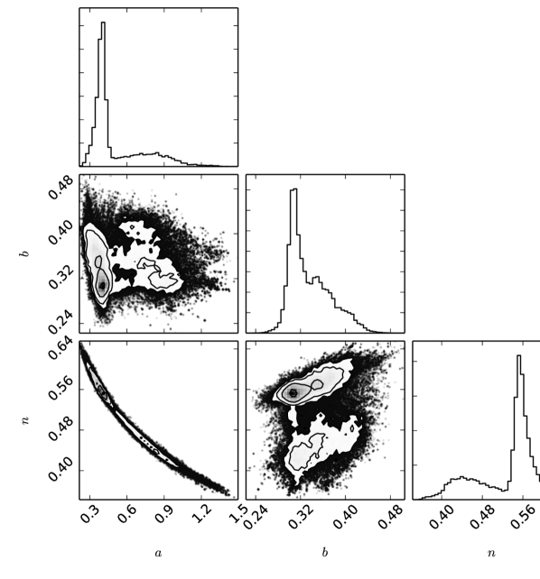
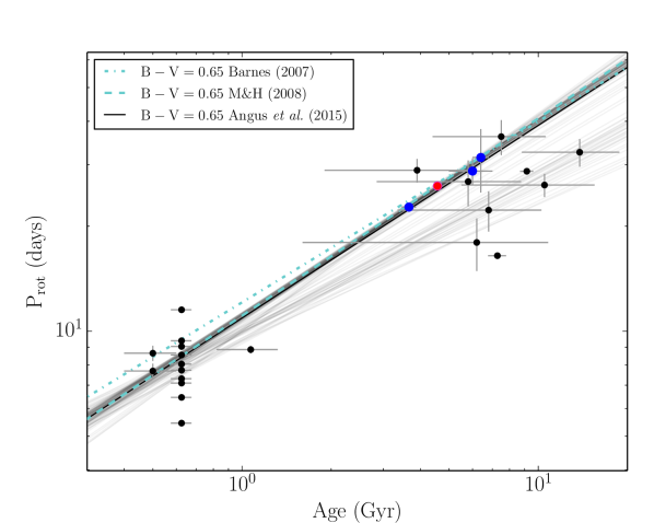
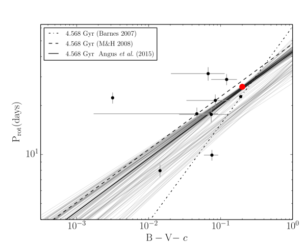
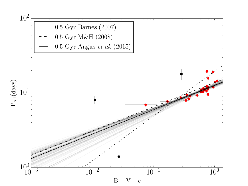
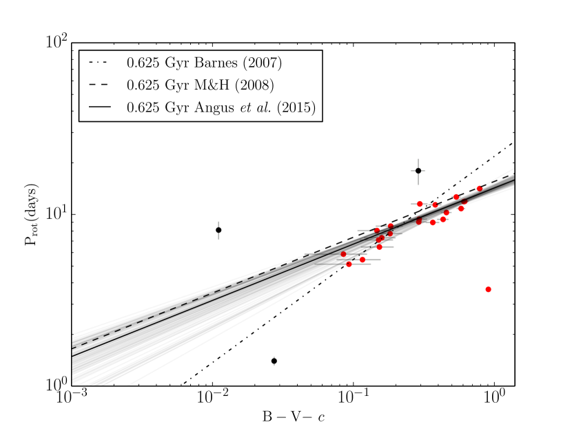
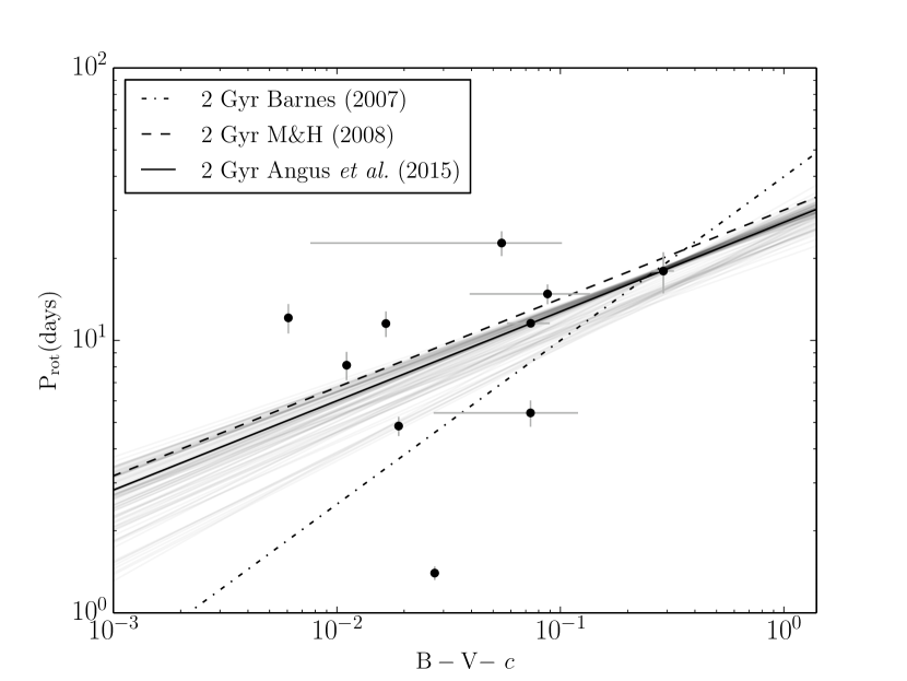
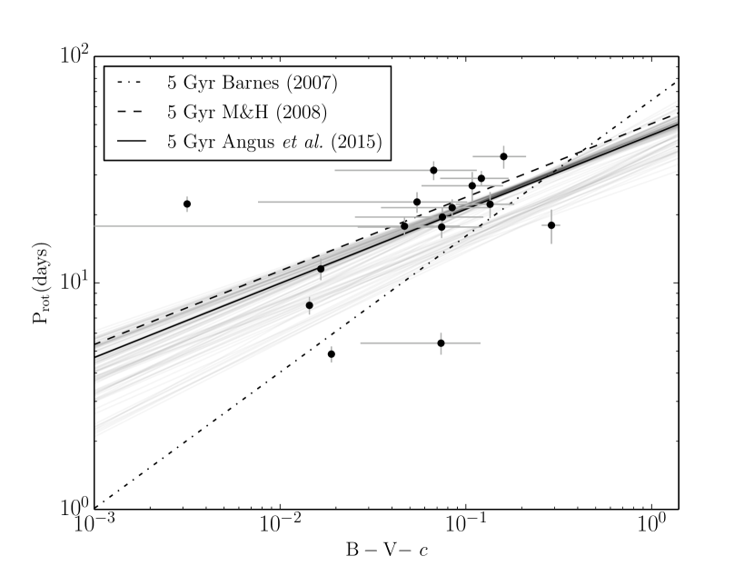
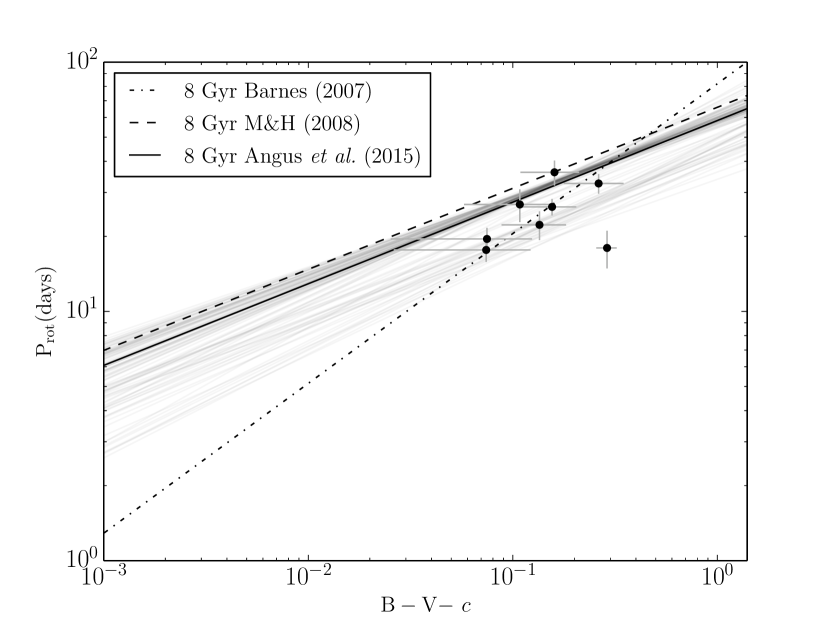
Figure 5 shows that parameters $a$ and $n$ are correlated and their posterior PDFs are bimodal. The position of the second peak falls around $a=0.8$, $b=0.34$ and $n=0.44$. The cause of this bimodality is clear when looking at the faint grey lines representing draws from the parameter posterior PDFs in figure 6. The majority of these draws fall close to the best-fitting model, which passes neatly through the Sun and field stars, however a significant fraction fall below the line of best-fit, passing through the Kepler asteroseismic stars which also mostly fall below the line. This result is reflected in Garcia et al. (2014) who model the AMP Kepler asteroseismic stars from Metcalfe et al. (2014), without anchoring their relation to the Sun. They find that the model that best describes the Kepler asteroseismic stars underpredicts the rotation period of the Sun. The grey lines that fall beneath our best-fitting model in figure 6 are drawn from the smaller peak in the posterior PDFs of $a$ and $n$ and seem to describe the relation between rotation period and age for the Kepler asteroseismic stars. In other words, the bimodal posterior PDFs of $a$ and $n$ are produced by the disagreement between the Kepler asteroseismic stars and the Sun and field stars. One set of gyrochronology parameters is not capable of describing the Sun, plus field stars, and the Kepler asteroseismic stars simultaneously. There is more than one possible explanation for this result. Firstly, the asteroseismic ages could be systematically biased high. Secondly, the rotation periods could be systematically underestimated. This could occur if, for example, these stars were rotating differentially and the dominant spotted regions on their surfaces were not equatorial. Thirdly, this could be a result of an observational bias produced by incomplete detection, sometimes known as Malmquist bias (Malmquist, 1920). If there were a large spread in rotation periods for a given stellar mass and age and, due to the detection bias brought about because shorter periods are easier to detect than longer periods, this broad range of rotation periods might be truncated at some upper cut-off. It would therefore appear as though Solar-colour stars were rotating too slowly for their age simply because only rapidly rotating Kepler stars appeared in our sample. Kepler systematics hinder our ability to measure longer rotation periods, but in addition, more slowly rotating stars tend to be less active, with fewer surface features and are therefore more likely to be missing from our sample. Finally, it is possible that the Kepler asteroseismic stars follow a different spin-down relation to the Sun and field stars, perhaps due to having different metallicities. Unfortunately it is not currently possible to identify the cause of the observed mismatch between the Kepler stars and the field stars and we leave this question for a future investigation.

The fact that our fit is so heavily dominated by the Sun with its small uncertainties is, perhaps, a cause for concern. We know the rotation period and age of the Sun very precisely, however, if the Sun is not exactly representative of a typical star, the resulting best-fit gyrochronology relation will also not represent typical stars. The field stars in our sample are well represented by the best-fit gyrochronology relation, which provides reassurance that the Sun is a typical star amongst this set. We did not attempt to tackle the problem of how to appropriately treat the Sun as a single, highly-precise data point in a sample that also contains imprecise data. Instead, we leave this problem for future consideration. Despite the fact that a lot of weight is attributed to the Sun because of its small uncertainties, this new gyrochronology relation is still the most representative, empirically calibrated relation between colour, rotation period and age for MS F, G and K stars to date.

Our final, newly calibrated gyrochronology relation can be written in full as

$$P=A^{0.55^{+0.02}_{-0.09}}\times 0.40^{+0.3}_{-0.05}(B-V-0.45)^{0.31^{+0.05}_{-0.02}},$$ (15)

with rotation period, $P$ in days and age, $A$ in Myr. An age can be calculated for a star with a rotation period and colour by inverting this relationship. Covariances between the gyrochronology parameters should be taken into account whenever the above relation is used to calculate uncertainties on an age or rotation period prediction. In order to do this properly, posterior PDF samples should be incorporated into Monte-Carlo uncertainty calculations.

In order to test the predictive power of the new gyrochronology relation, we inverted equation 15 to compare previously measured ages with new age predictions for the 6 field stars (see table 6). For comparison, gyrochronological ages for the field stars were also computed using the relations of Barnes (2007) and Mamajek & Hillenbrand (2008). Uncertainties on ages predicted with the new relation were calculated using posterior PDF samples of the three parameters, $a$, $b$ and $n$.

Table 6: Field star ages taken from the literature, compared with predictions from this work (1), Mamajek & Hillenbrand (2008) (2) and Barnes (2007) (3).

Star	Literature age (Gyr)	Age 1 (Gyr)	Age 2 (Gyr)	Age 3 (Gyr)
18 Sco	$3.7\pm 0.2$	$3.7^{+2.5}_{-0.3}$	$3.5^{+0.6}_{-0.5}$	$3.7^{+0.8}_{-0.6}$
The Sun	$4.568\pm 0.001$	$4.6^{+3.5}_{-0.3}$	$4.7^{+0.7}_{-0.6}$	$4.8^{+1}_{-0.8}$
Alpha Cen A	$6.0\pm 1$	$5.0^{+3.3}_{-1.0}$	$4.5^{+1}_{-0.9}$	$5\pm 1$
Alpha Cen B	$6.0\pm 1$	$6.0^{+3.8}_{-1.7}$	$4^{+1}_{-0.9}$	$5^{+2}_{-1}$
16 Cyg A	$6.8\pm 0.4$	$4.0^{+2.6}_{-0.7}$	$3\pm 2$	$4\pm 2$
16 Cyg B	$6.8\pm 0.4$	$3.7^{+3.4}_{-2.1}$	$3\pm 2$	$4\pm 2$

The ages predicted by the three different relations are consistent within uncertainties, with the exception of Alpha Cen B. All three relations underpredict the age of the 16 Cyg system. The rotation periods of both 16 Cyg A and B used in this paper are asteroseismic measurements of the internal (not surface) rotation periods of the stars. If the stars’ cores are rotating much more rapidly than their surfaces, this could account for this age discrepancy.

The goal of gyrochronology in general is to provide a means of predicting the age of a star given observations of its colour (or mass, or temperature), and rotation period. The discrepancies in period-colour relations between clusters, Kepler stars and nearby field stars in the above analysis does not bode well for the current, simple gyrochronology model. Until now it has been hoped that one single relation between period, mass and age could be used to describe all F, G and K MS stars. Even though we are unable to identify the cause of the discrepancy between the Kepler stars and the field stars, a different gyrochronology relation still seems to be required for each cluster.

The ‘narrowness’ of the gyrochronology relation has hitherto been an unknown; do the three properties, age, mass and rotation period, truly lie on an infinitely narrow plane? Unfortunately we cannot fully answer this question here as the asteroseismic ages are noisy and observational and intrinsic scatter are ambiguously interwoven. However, if this sample of stars is subject to Malmquist bias then, by definition, there must be a broad range of rotation periods for stars of a given mass and age. A future study might include an extra parameter that describes the ‘width’ of the gyrochronological plane and attempt to detect an element of scatter above the noise level. Does age depend solely on rotation period and mass or do other variables influence stellar spin down, perhaps only becoming important after many Myrs? The gyrochronology model calibrated here neglects the effects of metallicity. This property is bound to have an effect on the angular momentum evolution of a star since it impacts internal stellar structure. A future study, investigating the impact of metallicity on rotational evolution will be essential for improving our ability to date stars using gyrochronology.

The picture of gyrochronology will become clearer as the sample of asteroseismic stars with individual mode analysis grows and their age uncertainties shrink. The best targets for asteroseismic studies are relatively inactive since they allow the easier detection of Solar-like oscillations. Inactive stars are also the best targets for gyrochronology as they are usually old and slowly rotating. However these targets are not well suited for rotation period measurements which are most easily and precisely determined for active, rapidly rotating stars. K2, the repurposed Kepler mission, will provide new targets for rotation studies; in particular, some relatively old clusters have been and will continue to be monitored by the spacecraft. The observing seasons of K2 are relatively short ($\sim$ 90 days) and fields will only be observed once, so the maximum rotation periods measurable from K2 light curves will be considerably shorter than with Kepler. However these clusters may still be extremely useful for gyrochronology.

5 Summary

We have calibrated the relation between rotation period, $B-V$ colour and age for MS stars with $T_{\rm{eff}}$$<$ 6250 K, using 310 Kepler asteroseismic targets, supplemented with 6 field stars and 50  cluster stars. Unlike previous gyrochronology calibrations, our sample covers a large range of ages, observational uncertainties on all parameters were accounted for and the posterior PDFs of model parameters were explored using MCMC. Incorporating observational uncertainties into the model fitting process was an essential component of our analysis since these uncertainties, particularly on the asteroseismic ages, were large. Three populations: hot dwarfs, cool dwarfs and subgiants, were modelled simultaneously in order to account for potential misclassifications that might have arisen from large observational uncertainties. Posterior probability distributions of the gyrochronology parameters were explored using MCMC and the impact of leaving out subsets of the sample was assessed, leading us to find that a single relation between rotation period, colour and age does not adequately describe the cluster data. For this reason, only the Hyades and Coma Berenices clusters were used to calibrate the model. Fitting equation 1 to the Hyades and Coma Berenices clusters, the Kepler asteroseismic stars, local field stars and the Sun resulted in bimodal posterior PDFs. The Kepler asteroseismic stars were not well described by the same gyrochronology relation as the Sun, field stars and clusters. There are several potential explanations for the cause of this phenomenon. Some of the most likely are: the asteroseismic ages or the photometric rotation periods could be systematically biased; the rotation periods might be subject to Malmquist bias due to incomplete detection; and the different populations could have different physical properties (e.g. metallicity), not accounted for in the gyrochronology model. If Malmquist bias is responsible and there truely is a broad range of rotation periods for stars of a given age and colour, this still has negative implications for Gyrochronology which relies on the assumption that these three properties lie on a neat plane.

The careful and well motivated modelling techniques used in this work allowed us to identify the potential shortcomings of the current gyrochronology model. Only by conducting MCMC parameter exploration and studying the resulting posterior PDFs were we able to see that one global gyrochronology relation cannot describe all subsets of our sample. The results are somewhat unsettling—no single model describes the sample as a whole, even when dropping some of the clusters and allowing for rather complex population subsets. This tells us that the current model is probably not good enough, but it - or something very similar - is the model everyone has been using in gyrochronology studies so far. Previous studies did not model multiple cluster and field populations simultaneously, or do the modelling in such a detailed way, so the problems didn’t come through so clearly. In the future better physical models may be developed, better ages may be calculated and more sensitive period search methods, not so susceptible to Malmquist bias may become available. When they do, the prescription we provide will enable the the period-colour-age relation to be modelled more sensitively.

The code used in this project can be found at https://github.com/RuthAngus/Gyro. R.A. acknowledges funding from the Leverhulme Trust. A.M. acknowledges funding from the European Research Council under the EU’s Seventh Framework Programme (FP7/(2007-2013)/ERC Grant Agreement No. 291352). We wish to thank the anonymous referee for their valuable and insightful feedback and Bill Chaplin for his thoughtful and detailed comments which enormously improved this paper. We would also like to thank Tsevi Maseh, Eric Mamajek, Daniel Mortlock and David Hogg for useful insight and discussion that hugely contributed to this paper.

References

- Barnes (2003) Barnes S. A., 2003, ApJ, 586, 464
- Barnes (2007) Barnes S. A., 2007, ApJ, 669, 1167
- Bazot et al. (2012) Bazot M., Bourguignon S., Christensen-Dalsgaard J., 2012, MNRAS, 427, 1847
- Bouvier & Wadhwa (2010) Bouvier A., Wadhwa M., 2010, Nature Geoscience, 3, 637
- Brown & Gilliland (1994) Brown T. M., Gilliland R. L., 1994, ARA&A, 32, 37
- Bruntt et al. (2012) Bruntt H., Basu S., Smalley B., et al., 2012, MNRAS, 423, 122
- Casagrande et al. (2010) Casagrande L., Ramírez I., Meléndez J., et al., 2010, A&A, 512, A54
- Chaplin et al. (2014) Chaplin W. J., Basu S., Huber D., et al., 2014, ApJS, 210, 1
- Collier Cameron et al. (2009) Collier Cameron A., Davidson V. A., Hebb L., et al., 2009, MNRAS, 400, 451
- Cox & Pilachowski (2000) Cox A. N., Pilachowski C. A., 2000, Physics Today, 53, 77
- Davies et al. (2014) Davies G. R., Chaplin W. J., Farr W. M., et al., 2014, ArXiv e-prints
- Demarque et al. (2004) Demarque P., Woo J.-H., Kim Y.-C., et al., 2004, ApJS, 155, 667
- Demory (2014) Demory B.-O., 2014, ApJ, 789, L20
- Dobbie et al. (2009) Dobbie P. D., Casewell S. L., Burleigh M. R., et al., 2009, MNRAS, 395, 1591
- Donahue et al. (1996) Donahue R. A., Saar S. H., Baliunas S. L., 1996, ApJ, 466, 384
- Dumusque et al. (2012) Dumusque X., Pepe F., Lovis C., et al., 2012, Nature, 491, 207
- Foreman-Mackey et al. (2013) Foreman-Mackey D., Hogg D. W., Lang D., et al., 2013, PASP, 125, 306
- Foreman-Mackey et al. (2014) Foreman-Mackey D., Hogg D. W., Morton T. D., 2014, ApJ, 795, 64
- Foreman-Mackey et al. (2014) Foreman-Mackey D., Price-Whelan A., Ryan G., et al., 2014
- Garcia et al. (2014) Garcia R. A., Ceillier T., Salabert D., et al., 2014, ArXiv e-prints
- Hallam et al. (1991) Hallam K. L., Altner B., Endal A. S., 1991, ApJ, 372, 610
- Hogg et al. (2010) Hogg D. W., Myers A. D., Bovy J., 2010, ApJ, 725, 2166
- Irwin & Bouvier (2009) Irwin J., Bouvier J., 2009, in Mamajek E. E., Soderblom D. R., Wyse R. F. G., eds, IAU Symposium Vol. 258 of IAU Symposium, The rotational evolution of low-mass stars. pp 363–374
- Kawaler (1988) Kawaler S. D., 1988, ApJ, 333, 236
- Kraft (1967) Kraft R. P., 1967, ApJ, 150, 551
- Krishnamurthi et al. (1998) Krishnamurthi A., Terndrup D. M., Pinsonneault M. H., et al., 1998, ApJ, 493, 914
- Li et al. (2012) Li T. D., Bi S. L., Liu K., et al., 2012, A&A, 546, A83
- Malmquist (1920) Malmquist K., 1920, Medd. Lund. Astron. Obs, 22, 1
- Mamajek & Hillenbrand (2008) Mamajek E. E., Hillenbrand L. A., 2008, ApJ, 687, 1264
- McQuillan et al. (2014) McQuillan A., Mazeh T., Aigrain S., 2014, ApJS, 211, 24
- Meibom et al. (2011) Meibom S., Mathieu R. D., Stassun K. G., et al., 2011, ApJ, 733, 115
- Mermilliod (1986) Mermilliod J.-C., 1986, Catalogue of Eggen’s UBV data., 0 (1986), p. 0
- Metcalfe et al. (2012) Metcalfe T. S., Chaplin W. J., Appourchaux T., et al., 2012, ApJ, 748, L10
- Metcalfe et al. (2014) Metcalfe T. S., Creevey O. L., Dogan G., et al., 2014, ArXiv e-prints
- Moffett & Barnes (1979) Moffett T. J., Barnes III T. G., 1979, PASP, 91, 180
- Morton & Winn (2014) Morton T. D., Winn J. N., 2014, ArXiv e-prints
- Noyes et al. (1984) Noyes R. W., Hartmann L. W., Baliunas S. L., Duncan D. K., Vaughan A. H., 1984, ApJ, 279, 763
- Paulson et al. (2004) Paulson D. B., Cochran W. D., Hatzes A. P., 2004, AJ, 127, 3579
- Perryman et al. (1998) Perryman M. A. C., Brown A. G. A., Lebreton Y., et al., 1998, A&A, 331, 81
- Petit et al. (2008) Petit P., Dintrans B., Solanki S. K., et al., 2008, MNRAS, 388, 80
- Pinsonneault et al. (2012) Pinsonneault M. H., An D., Molenda-Zakowicz J., et al., 2012, VizieR Online Data Catalog, 219, 90030
- Prosser et al. (1995) Prosser C. F., Shetrone M. D., Dasgupta A., et al., 1995, PASP, 107, 211
- Radick et al. (1995) Radick R. R., Lockwood G. W., Skiff B. A., Thompson D. T., 1995, ApJ, 452, 332
- Radick et al. (1987) Radick R. R., Thompson D. T., Lockwood G. W., et al., 1987, ApJ, 321, 459
- Rogers (2014) Rogers L. A., 2014, ArXiv e-prints
- Sekiguchi & Fukugita (2000) Sekiguchi M., Fukugita M., 2000, AJ, 120, 1072
- Silva Aguirre et al. (2013) Silva Aguirre V., Basu S., Brandão I. M., et al., 2013, ApJ, 769, 141
- Silva Aguirre et al. (2012) Silva Aguirre V., Casagrande L., Basu S., et al., 2012, ApJ, 757, 99
- Silva Aguirre et al. (2011) Silva Aguirre V., Chaplin W. J., Ballot J., et al., 2011, ApJ, 740, L2
- Skumanich (1972) Skumanich A., 1972, ApJ, 171, 565
- Soderblom (2010) Soderblom D. R., 2010, ARA&A, 48, 581
- van Saders & Pinsonneault (2013) van Saders J. L., Pinsonneault M. H., 2013, ApJ, 776, 67
- Weber & Davis (1967) Weber E. J., Davis Jr. L., 1967, ApJ, 148, 217
- Yıldız (2007) Yıldız M., 2007, MNRAS, 374, 1264