Phase Transitions for High Dimensional Clustering and Related Problems

Abstract

Consider a two-class clustering problem where we observe $X_{i}=\ell_{i}\mu+Z_{i}$, $Z_{i}\stackrel{{\scriptstyle iid}}{{\sim}}N(0,I_{p})$, $1\leq i\leq n$. The feature vector $\mu\in R^{p}$ is unknown but is presumably sparse. The class labels $\ell_{i}\in\{-1,1\}$ are also unknown and the main interest is to estimate them.

We are interested in the statistical limits. In the two-dimensional phase space calibrating the rarity and strengths of useful features, we find the precise demarcation for the Region of Impossibility and Region of Possibility. In the former, useful features are too rare/weak for successful clustering. In the latter, useful features are strong enough to allow successful clustering. The results are extended to the case of colored noise using Le Cam’s idea on comparison of experiments.

We also extend the study on statistical limits for clustering to that for signal recovery and that for global testing. We compare the statistical limits for three problems and expose some interesting insight.

We propose classical PCA and Important Features PCA (IF-PCA) for clustering. For a threshold $t>0$, IF-PCA clusters by applying classical PCA to all columns of $X$ with an $L^{2}$-norm larger than $t$. We also propose two aggregation methods. For any parameter in the Region of Possibility, some of these methods yield successful clustering.

We discover a phase transition for IF-PCA. For any threshold $t>0$, let $\xi^{(t)}$ be the first left singular vector of the post-selection data matrix. The phase space partitions into two different regions. In one region, there is a $t$ such that $\mathrm{cos}(\xi^{(t)},\ell)\rightarrow 1$ and IF-PCA yields successful clustering. In the other, $\mathrm{cos}(\xi^{(t)},\ell)\leq c_{0}<1$ for all $t>0$.

Our results require delicate analysis, especially on post-selection Random Matrix Theory and on lower bound arguments.

, , and

1 Introduction

Motivated by the interest on gene microarray study, we consider a clustering problem where we have $n$ subjects from two different classes (e.g., normal and diseased), measured on the same set of $p$ features (i.e., gene expression level). To facilitate the analysis, we assume that two classes are equally likely so the class labels satisfy

$$\ell_{i}\stackrel{{\scriptstyle iid}}{{\sim}}2\mathrm{Bernoulli}(1/2)-1,\qquad 1\leq i\leq n.$$ (1.1)

We also assume that the $p$-dimensional data vectors $X_{i}$’s are standardized, so that for a contrast mean vector $\mu\in R^{p}$,

$$X_{i}=\ell_{i}\mu+Z_{i},\qquad Z_{i}\stackrel{{\scriptstyle iid}}{{\sim}}N(0,I_{p}),\qquad 1\leq i\leq n.$$ (1.2)

Throughout this paper, we call feature $j$, $1\leq j\leq p$, a “useless feature” or “noise” if $\mu(j)=0$ and a “useful feature” or “signal” otherwise.

The paper focuses on the problem of clustering (i.e., estimating the class labels $\ell_{i}$). Such a problem is of interest, especially in the study of complex disease [35]. In the two-dimensional phase space calibrating the signal rarity and signal strengths, we are interested in the following limits.

• Statistical limits. This is the precise boundary that separates the Region of Impossibility and Region of Possibility. In the former, the signals are so rare and (individually) weak that it is impossible for any method to correctly identify most of the class labels. In the latter, the signals are strong enough to allow successful clustering, and it is desirable to develop methods that cluster successfully.

• Computationally tractable statistical limits. This is similar to the boundary above, except that for both Possibility and Impossibility, we only consider statistical methods that are computationally tractable.

We use Region of Possibility and Region of Impossibility as generic terms, which may vary from occurrence to occurrence.

The paper also contains three closely related objectives as follows, which we discuss in Sections 1.4 and 2, Section 3, and Section 4, respectively.

• Performance of the recent idea of Important Features PCA (IF-PCA).

• Limits for recovering the support of $\mu$ (signal recovery).

• Limits for testing whether $X_{i}$’s are iid samples from $N(0,I_{p})$, or generated from Model (1.2) (hypothesis testing).

Our work on sparse clustering is related to Azizyan et al [7] and Chan and Hall [13] (see also [38, 39, 43, 49]): the three papers share the same spirit that we should do a feature selection before we cluster. Our work on support recovery is related to recent interest on sparse PCA (e.g., Amini and Wainwright [3], Johnstone and Lu [32], Vu and Lei [46], Wang et al [47], Arias-Castron and Verzelen [5]), and our work on hypothesis testing is related to recent interest on matrix estimation and matrix testing (e.g., Arias-Castro and Verzelen [5], Cai et al [11]). However, our work is different in many important aspects, especially for our focus on the limits and on the Rare/Weak models. See Section 6 for more discussion.

1.1 Four clustering methods

Denoting the data matrix by $X$, we write

$$X^{\prime}=[X_{1},X_{2},\ldots,X_{n}],\qquad X=[x_{1},x_{2},\ldots,x_{p}].$$

We introduce two methods: a feature aggregation method and IF-PCA. Each method includes a special case, which can be viewed as a different method.

The first method $\hat{\ell}^{(sa)}_{N}$ targets on the case where the signals are rare but individually strong (“sa”: Sparse Aggression; $N$: tuning parameter; usually, $N\ll p$), so feature selection is desirable. Denote the support of $\mu$ by

$$S(\mu)=\{1\leq j\leq p:\mu(j)\neq 0\}.$$ (1.3)

The procedure first estimates $S(\mu)$ by optimizing ($\|\cdot\|_{1}$: vector $L^{1}$-norm)

$$\hat{S}^{(sa)}_{N}=\mathrm{argmax}_{\{S\subset\{1,2,\ldots,p\}:|S|=N\}}\bigl{\{}\|\sum\nolimits_{j\in S}x_{j}\|_{1}\bigr{\}},$$ (1.4)

and then cluster by aggregating all selected features $\hat{\ell}^{(sa)}_{N}=\hbox{\rm sgn}\bigl{(}\sum\nolimits_{j\in\hat{S}^{(sa)}_{N}}x_{j}\bigr{)}$.

An important special case is $N=p$, where $\hat{\ell}_{N}^{(sa)}$ reduces to the method of Simple Aggregation which we denote by $\hat{\ell}_{*}^{(sa)}$. This procedure targets on the case where the signals are weak but less sparse, so feature selection is hopeless. Note that $\hat{\ell}_{N}^{(sa)}$ is generally NP-hard but $\hat{\ell}_{*}^{(sa)}$ is not.

The second method is IF-PCA, denoted by $\hat{\ell}_{q}^{(if)}$, where $q>0$ is a tuning parameter. The method targets on the case where the signals are rare but individually strong. To use $\hat{\ell}_{q}^{(if)}$, we first select features using the $\chi^{2}$-tests:

$$\hat{S}^{(if)}_{q}=\{1\leq j\leq p:Q(j)\geq\sqrt{2q\log(p)}\},\;\;Q(j)=(\|x_{j}\|^{2}-n)/\sqrt{2n}.$$ (1.5)

We then obtain the first left singular vector $\xi^{(q)}$ of the post-selection data matrix $X^{(q)}$ (containing only columns of $X$ where the indices are in $\hat{S}^{(if)}_{q}$):

$$\xi^{(q)}=\xi(X^{(q)}),$$ (1.6)

and cluster by $\hat{\ell}_{q}^{(if)}=\hbox{\rm sgn}(\xi^{(q)})$. IF-PCA includes the classical PCA (denoted by $\hat{\ell}_{*}^{(if)}$) as a special case, where the feature selection step is skipped, and $\xi^{(q)}$ reduces to the first singular vector of $X$.

In Table 1, we compare all four methods. Note that for more complicated cases (e.g., the nonzero $\mu(j)$’s may be both positive and negative), we may consider a variant of $\hat{\ell}_{N}^{(sa)}$ which clusters by $\hat{\ell}_{N}^{(sa)}=\hbox{\rm sgn}(X\hat{\mu})$, with $\hat{\mu}$ being $\mathrm{argmax}_{\{\mu(j)\in\{-1,0,1\},\|\mu\|_{0}=N\}}\|X\mu\|_{q}$, where $q>0$. If we let $q=1$ and restrict $\mu(j)\in\{0,1\}$, it reduces to the current $\hat{\ell}_{N}^{(sa)}$. Note that when $N=p$ and $q=2$, approximately, $\hat{\mu}$ is proportional to the first right singular vector of $X$ and $\hat{\ell}_{N}^{(sa)}$ is approximately the classical PCA. Note also that $\hat{\ell}_{q}^{(if)}$ can be viewed as the adaption of IF-PCA in Jin and Wang [31] to Model (1.2). The version in [31] is a tuning free algorithm for analyzing microarray data and is much more sophisticated. The current version of IF-PCA is similar to that in Johnstone and Lu [32] but is also different in purpose and in implementation: the former is for estimating $\ell$ and uses the first left singular vector of the post-selection data matrix, and the latter is for estimating $\mu$ and uses the first right singular vector. The theory two methods entail are also very different. See Sections 1.8 and 6 for more discussion.

Table 1: Comparison of basic characteristics of four methods. *: signals are comparably stronger but still weak. $\dagger$: a tuning-free version exists.

Methods	Simple Aggregation	Sparse Aggregation	Classical PCA	IF-PCA
	$\hat{\ell}_{*}^{(sa)}$	$\hat{\ell}_{N}^{(sa)}$ ($N\ll p$)	$\hat{\ell}_{*}^{(if)}$	$\hat{\ell}_{q}^{(if)}(q>0)$
Signals	less sparse/weak	sparse/strong*	moderately sparse/weak	very sparse/strong
Feature selection	No	Yes	No	Yes
Comp. complexity	Polynomial	NP-hard	Polynomial	Polynomial
Need tuning	No	Yes	No	Yes$\dagger$

1.2 Rare and Weak signal model

To study all these limits, we invoke the Asymptotic Rare and Weak (ARW) model [12, 19, 20, 26]. In ARW, for two parameters $(\epsilon,\tau)$, we model the contrast mean vector $\mu$ by

$$\mu(j)\stackrel{{\scriptstyle iid}}{{\sim}}(1-\epsilon)\nu_{0}+\epsilon\nu_{\tau},\qquad 1\leq j\leq p,$$ (1.7)

where $\nu_{a}$ denotes the point mass at $a$. In Model (1.7), all signals have the same sign and magnitude. Such an assumption can be largely relaxed; see Sections 1.6 and 6. We use $p$ as the driving asymptotic parameter and tie $(n,\epsilon,\tau)$ to $p$ by fixed parameters. In detail, fixing $(\theta,\beta)\in(0,1)^{2}$ and $\alpha>0$, we model

$$n=n_{p}=p^{\theta},\qquad\epsilon=\epsilon_{p}=p^{-\beta},\qquad\tau=\tau_{p}=p^{-\alpha}.$$ (1.8)

In our model, $n\ll p$ for we focus on the modern “large $n$, really large $p$” regime [42]. The study can be conveniently extended to the case of $n\gg p$.

1.3 Limits for clustering

Let $\Pi$ be the set of all possible permutations on $\{-1,1\}$. For any clustering procedure $\hat{\ell}$ (where $\hat{\ell}_{i}$ takes values from $\{-1,1\}$), we measure the performance by the Hamming distance:

$$\mathrm{Hamm}_{p}(\hat{\ell},\alpha,\beta,\theta)=n^{-1}\inf_{\pi\in\Pi}\biggl{\{}\sum_{i=1}^{n}P(\hat{\ell}_{i}\neq\pi\ell_{i})\biggr{\}},$$ (1.9)

where the probability is evaluated with respective to $(\mu,\ell,Z)$. Fixing $\theta\in(0,1)$, introduce a curve $\alpha=\eta^{clu}_{\theta}(\beta)$ in the $\beta$-$\alpha$ plane by

$$\eta^{clu}_{\theta}(\beta)=\left\{\begin{array}[]{ll}(1-2\beta)/2,&\qquad\beta<(1-\theta)/2,\\ \theta/2,&\qquad(1-\theta)/2<\beta<(1-\theta),\\ (1-\beta)/2,&\qquad\beta>(1-\theta).\end{array}\right.$$

Theorem 1.1

(Statistical lower bound). Fix $(\theta,\beta)\in(0,1)^{2}$ and $\alpha>0$ such that $\alpha>\eta^{clu}_{\theta}(\beta)$. Consider the clustering problem for Models (1.1)-(1.2) and (1.7)-(1.8). For any procedure $\hat{\ell}$, $\lim\inf_{p\rightarrow\infty}\mathrm{Hamm}_{p}(\hat{\ell},\alpha,\beta,\theta)\geq 1/2$.

Theorem 1.2

(Statistical upper bound for clustering). Fix $(\theta,\beta)\in(0,1)^{2}$ and $\alpha>0$ such that $\alpha<\eta^{clu}_{\theta}(\beta)$, and consider the clustering problem for Models (1.1)-(1.2) and (1.7)-(1.8). As $p\rightarrow\infty$,

• $\mathrm{Hamm}_{p}(\hat{\ell}_{*}^{(sa)},\alpha,\beta,\theta)\rightarrow 0$, if $0<\beta<(1-\theta)/2$.

• $\mathrm{Hamm}_{p}(\hat{\ell}_{N}^{(sa)},\alpha,\beta,\theta)\rightarrow 0$, if $(1-\theta)/2<\beta<1$ and $N=\lceil p\epsilon_{p}\rceil$.

As a result, the curve $\alpha=\eta^{clu}_{\theta}(\beta)$ divides the $\beta$-$\alpha$ plane into two regions: Region of Impossibility and Region of Possibility. In the former, the signals are so weak that successful clustering is impossible. In the latter, the signals are strong enough to allow successful clustering.

Consider computationally tractable limits. We call a curve $r=\eta_{\theta}(\beta)$ in the $\beta$-$\alpha$ plane a Computationally Tractable Upper Bound (CTUB) if for any fixed $(\theta,\alpha,\beta)$ such that $\alpha<\eta_{\theta}(\beta)$, there is a computationally tractable clustering method $\hat{\ell}$ such that $\mathrm{Hamm}_{p}(\hat{\ell},\alpha,\beta,\theta)\rightarrow 0$. A CTUB $r=\eta_{\theta}(\beta)$ is tight if for any computationally tractable method $\hat{\ell}$ and any fixed $(\theta,\alpha,\beta)$ such that $\alpha>\eta_{\theta}(\beta)$, $\lim\inf_{p\rightarrow\infty}\mathrm{Hamm}_{p}(\hat{\ell},\alpha,\beta,\theta)\geq 1/2$. In this case, we call $r=\eta_{\theta}(\beta)$ the Computationally Tractable Boundary (CTB). Define

$$\tilde{\eta}^{clu}_{\theta}(\beta)=\left\{\begin{array}[]{ll}(1-2\beta)/2,&\qquad\beta<(1-\theta)/2,\\ (1+\theta-2\beta)/4,&\qquad(1-\theta)/2<\beta<1/2,\\ \theta/4,&\qquad 1/2<\beta<1-\theta/2,\\ (1-\beta)/2,&\qquad 1-\theta/2<\beta<1.\end{array}\right.$$

Theorem 1.3

(A CTUB for clustering). Fix $(\theta,\beta)\in(0,1)^{2}$ and $\alpha>0$ such that $\alpha<\tilde{\eta}^{clu}_{\theta}(\beta)$, and consider the clustering problem for Models (1.1)-(1.2) and (1.7)-(1.8). As $p\rightarrow\infty$,

• $\mathrm{Hamm}_{p}(\hat{\ell}_{*}^{(sa)},\alpha,\beta,\theta)\rightarrow 0$, if $0<\beta<(1-\theta)/2$.

• $\mathrm{Hamm}_{p}(\hat{\ell}_{*}^{(if)},\alpha,\beta,\theta)\rightarrow 0$, if $(1-\theta)/2<\beta<1/2$.

• $\mathrm{Hamm}_{p}(\hat{\ell}_{q}^{(if)},\alpha,\beta,\theta)\rightarrow 0$, if $1/2<\beta<1$ and we take $q\geq 3$.

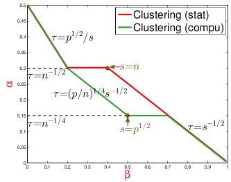
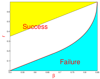
Figure 1: Left: the statistical limits (red) and the CTUB (green) for clustering ($s=p\epsilon_{p}$ is the expected number of signals). Right: phase transition of IF-PCA. White region: successful clustering is possible but successful feature selection is impossible (using column-wise $\chi^{2}$ scores). Yellow region: both successful clustering and feature selection are possible.

We now discuss CTB. We discuss the cases (a) $0<\beta<(1-\theta)/2$, (b) $(1-\theta)/2<\beta<1/2$, (c) $1/2<\theta<1-\theta/2$, and (d) $1-\theta/2<\beta<1$ separately. Note that the CTB is sandwiched by two curves $\alpha=\eta^{clu}_{\theta}(\beta)$ and $\alpha=\tilde{\eta}_{\theta}^{clu}(\beta)$. In (a) and (d), $\tilde{\eta}^{clu}_{\theta}(\beta)=\eta^{clu}_{\theta}(\beta)$, so our CTUB (i.e., CTUB given in Theorem 1.3) is tight. For (b), we are not sure but we conjecture that our CTUB is tight. For (c), we have good reasons to believe that our CTUB is tight. In fact, our model is intimately connected to the spike model [32]; see Section 1.8. The tightness of our CTUB under the spike model has been well-studied (e.g., [9, 37]). Translating their results to our setting suggests that there is a small constant $\delta>0$ such that when $1/2<\beta<1/2+\delta$, our CTUB is tight. Note that for (c), the CTUB $\alpha=\tilde{\eta}_{\theta}^{clu}(\beta)$ is flat. By the monotonicity of CTB (see below), our CTUB is tight for (c). See Figure 1.

Remark (Monotonicity of CTB). We show the CTB is monotone in $\beta$ (with $\theta$ fixed). Fix $\delta>0$ and consider a new experiment, where for each column of the data matrix, we keep the column with probability $p^{-\delta}$ and replace it with an independent column drawn from $N(0,I_{n})$ with probability $1-p^{-\delta}$. Compare this with the original experiment. The parameters $(\alpha,\theta)$ are the same, but $\beta$ has become $(\beta+\delta)$. The second experiment is harder, for it is the result of the original experiment by sub-sampling the columns. This shows that the CTB is monotone in $\beta$. The monotonicity now follows by Le Cam’s results on comparison of experiments [34].

1.4 Phase transition for IF-PCA

IF-PCA is a flexible clustering method that is easy to use and computationally efficient. In [31], we developed a tuning free version of IF-PCA using Higher Criticism [19, 21, 27] and applied it to $10$ microarray data sets with satisfactory results. The success of IF-PCA in real data analysis motivates us to investigate the method in depth. To facilitate delicate analysis, we consider the version of IF-PCA in Section 1.1, and reveal an interesting phase transition.

To this end, we investigate a very challenging case (not covered in Theorems 1.1-1.3) where $(\alpha,\beta)$ fall exactly on the CTUB in Theorem 1.3:

$$\alpha=\tilde{\eta}_{\theta}^{clu}(\beta).$$ (1.10)

Also, note that a key step in IF-PCA is the column-wise $\chi^{2}$-screening. In our model, a column $x_{j}$ is either distributed as $N(0,I_{n})$ or $N(\tau_{p}\ell,I_{n})$, where $\tau_{p}=p^{-\alpha}$. For the $\chi^{2}$-screening to be non-trivial, we further require that

$$1/2<\beta<1-\theta/2.$$ (1.11)

For $\beta$ in this range, the curve $\alpha=\tilde{\eta}_{\theta}^{clu}(\beta)$ is flat, i.e., $\tilde{\eta}_{\theta}^{clu}(\beta)\equiv\theta/4$, and so $\tau_{p}=p^{-\theta/4}=n^{-1/4}$. For $\beta$ outside this range, (1.10) dictates that either $\tau_{p}\ll n^{-1/4}$ (so that the signals are too weak that the $\chi^{2}$-screening bounds to fail) or $\tau_{p}\gg n^{-1/4}$ (so that the signals are too strong that the $\chi^{2}$-screening is relatively trivial). See Figure 1.

We now restrict our attention to (1.10)-(1.11), where we recall that $\tau_{p}=p^{-\theta/4}$. To make the case more interesting, we adjust the calibration of $\tau_{p}$ slightly by an $O(\log^{1/4}(p))$ factor:

$$\tau_{p}^{*}=p^{-\theta/4}(4r\log(p))^{1/4},\;\;\;\mbox{where $0<r<1$ is a fixed parameter}.$$ (1.12)

With this calibration, the $\chi^{2}$-screening could be successful but non-trivial.

Introduce the standard phase function [19, 20]

$$\rho^{*}(\beta)=\left\{\begin{array}[]{ll}\beta-1/2,&\qquad 1/2<\beta<3/4,\\ (1-\sqrt{1-\beta})^{2},&\qquad 3/4<\beta<1.\end{array}\right.$$ (1.13)

Define the phase function for IF-PCA by

$$\rho_{\theta}^{*}(\beta)=(1-\theta)\cdot\rho^{*}\Big{(}1/2+\frac{\beta-1/2}{1-\theta}\Big{)},\qquad 1/2<\beta<1-\theta/2.$$ (1.14)

For any two vectors $x$ and $y$ in $R^{n}$, let $\mathrm{cos}(x,y)=\bigl{|}\langle x/\|x\|,y/\|y\|\rangle\bigr{|}$.

Theorem 1.4

(Phase transition for IF-PCA). Fix $(\theta,\beta,\alpha,r)\in(0,1)^{4}$ and $q>0$ such that (1.10)-(1.11) hold. Consider IF-PCA $\hat{\ell}_{q}^{(if)}$ for Models (1.1)-(1.2) and (1.7)-(1.8), where $\tau_{p}$ is replaced by the new calibration $\tau_{p}^{*}$ in (1.12), and let $\xi^{(q)}$ be the leading left singular vector as in (1.6). As $p\rightarrow\infty$,

• If $r>\rho_{\theta}^{*}(\beta)$, then with probability at least $1-o(p^{-2})$, $\mathrm{cos}(\xi^{(q^{*})},\ell)\rightarrow 1$ with $q^{*}=(\beta-\theta/2+r)^{2}/(4r)$ for $r>(\beta-\theta/2)/3$ and $q^{*}=4r$ otherwise.

• If $r<\rho_{\theta}^{*}(\beta)$, then with probability at least $1-o(n^{-1})$, there is a constant $c_{0}\in(0,1)$ such that $\mathrm{cos}(\xi^{(q)},\ell)\leq c_{0}$ for any fixed $0<q<1$.

Theorem 1.4 is proved in Section 2, using delicate spectral analysis on the post-selection data matrix (and so the term of post-selection Random Matrix Theory (RMT)). Compared to many works on RMT where the data matrix has independent entries [45], the entries of the post-selection data matrix are complicatedly correlated, so the required analysis is more delicate. We conjecture that when $r<\rho_{\theta}^{*}(\beta)$, $\mathrm{cos}(\xi^{(q)},\ell)\rightarrow 0$ for any fixed $0<q<1$. For now, we can only show this for $q$ in a certain range; see the proof for details.

Figure 1 (right) displays the phase diagram for IF-PCA. For fixed $(\alpha,\beta)$ in the interior of the white region, successful feature selection is impossible (by column-wise $\chi^{2}$-screening) but successful clustering is possible. This shows that feature selection and clustering are related but different problems.

Remark. For the IF-PCA considered here, we use column-wise $\chi^{2}$-tests for screening which is computationally inexpensive. Alternatively, we may use some regularization methods for screening (e.g., [15, 36, 50]). However, these methods are computationally more expensive, need tuning parameters that are hard to set, and are designed for feature selection, not clustering. For these reasons, it is unclear whether such alternatives may really help.

1.5 Clustering when the noise is colored

Consider a new version of ARW where $(\ell,\mu)$ are the same as in Models (1.1), (1.7)-(1.8), but Model (1.2) is replaced by a colored noise model

$$X=\ell\mu^{\prime}+AZB,\qquad Z_{i}(j)\stackrel{{\scriptstyle iid}}{{\sim}}N(0,1),\qquad 1\leq i\leq n,\;1\leq j\leq p,$$ (1.15)

where $A$ and $B$ are two non-random matrices.

Definition 1.1

We use $L_{p}>0$ to denote a generic multi-$\log(p)$ term which may vary from occurrence to occurrence such that for any fixed $\delta>0$, $L_{p}p^{-\delta}\rightarrow 0$ and $L_{p}p^{\delta}\rightarrow\infty$, as $p\rightarrow\infty$.

Theorem 1.5

(Statistical lower bound for clustering with colored noise). Consider the ARW model (1.1)-(1.2) and (1.7)-(1.8). Theorem 1.1 continues to hold if we replace the model (1.2) by (1.15) where $\max\{\|A\|,\|A^{-1}\|\}\leq L_{p}$ and $\max\{\|B\|,\|B^{-1}\|\}\leq L_{p}$.

Theorem 1.5 is proved in Section 5, using Le Cam’s comparison of experiments [34]. The idea is to construct a new experiment that is easy to analyze and that the current one can be viewed as the result of adding noise to it. Since “adding noise always makes the inference harder”, analyzing the new experiment provides a lower bound we need for the current experiment. The idea has been used in Hall and Jin [24], but for very different settings.

Consider the case $A=I_{n}$. In this case, the matrix $AZB$ has independent rows (but the columns may be correlated and heteroscedastic), and all four methods we proposed earlier continue to work, except that in IF-PCA we need $q\geq 3\max\{\mathrm{diag}(B^{\prime}B)\}$. The following theorem is proved in Section 3.

Theorem 1.6

(Upper bounds for clustering with colored noise). Consider the ARW model (1.1)-(1.2) and (1.7)-(1.8). Theorems 1.2-1.3 continue to hold if we replace the model (1.2) by (1.15) with $A=I_{n}$ and $B$ such that $\max\{\|B\|,\|B^{-1}\|\}\leq L_{p}$ and that all diagonals of $B^{\prime}B$ is upper bounded by a constant $c>0$, where we set $q\geq 3c$ in IF-PCA.

Practically, it is desirable to have a method that does not depend on the unknown parameter $c$. One way to attack this is to replace the column-wise $\chi^{2}$-test by a plug-in $\chi^{2}$-test where we estimate the variance column-wise by Median Absolute Deviation (say). However, such methods usually involve statistics of higher order moments; see [5] for discussions along this line.

1.6 Limits for signal recovery and hypothesis testing

For a more complete picture, we study the limits for signal recovery and hypothesis testing.

The goal of signal recovery is to recover the support of $\mu$. For any feature selector $\hat{S}$, we measure the error by the (normalized) Hamming distance $\mathrm{Hamm}_{p}(\hat{S},\alpha,\beta,\theta)=(p\epsilon_{p})^{-1}\sum_{j=1}^{p}[P(\mu(j)=0,j\in\hat{S})+P(\mu(j)\neq 0,j\notin\hat{S})]$, where $p\epsilon_{p}$ is the expected number of signals. Define

$$\eta^{sig}_{\theta}(\beta)=\left\{\begin{array}[]{ll}\theta/2,&\qquad\beta<(1-\theta),\\ (1+\theta-\beta)/4,&\qquad\beta>(1-\theta),\end{array}\right.$$

and

$$\tilde{\eta}^{sig}_{\theta}(\beta)=\left\{\begin{array}[]{ll}\theta/2,&\qquad\beta<(1-\theta)/2,\\ (1+\theta-2\beta)/4,&\qquad(1-\theta)/2<\beta<1/2,\\ \theta/4,&\qquad\beta>1/2.\end{array}\right.$$

The curve $r=\eta_{\theta}^{sig}(\beta)$ can be viewed as the counterpart of $r=\eta_{\theta}^{clu}(\beta)$, which divides the two-dimensional phase space into the Region of Impossibility and Region of Possibility. For any fixed $(\beta,\alpha)$ in the former and any $\hat{S}$, $\mathrm{Hamm}_{p}(\hat{S},\alpha,\beta,\theta)\gtrsim 1$. For any fixed $(\beta,\alpha)$ in the latter, there is an $\hat{S}$ such that $\mathrm{Hamm}_{p}(\hat{S},\alpha,\beta,\theta)\rightarrow 0$. The curve $r=\tilde{\eta}_{\theta}^{sig}(\beta)$ can be viewed as the counterpart of $r=\tilde{\eta}_{\theta}^{clu}(\beta)$ and provides a CTUB for the signal recovery problem. See Section 3 for more discussion.

The goal of (global) hypothesis testing is to test a null hypothesis $H_{0}^{(p)}$ that the data matrix $X$ has iid entries from $N(0,1)$ against an alternative hypothesis $H_{1}^{(p)}$ that $X$ is generated according to Model (1.2). Define

$$\eta_{\theta}^{hyp}(\beta)=\max\{\eta_{\theta}^{hyp,1}(\beta),\eta_{\theta}^{hyp,2}(\beta)\},\;\;\tilde{\eta}_{\theta}^{hyp}(\beta)=\max\{\eta_{\theta}^{hyp,1}(\beta),\frac{\theta}{4}\},$$ (1.16)

and $\eta_{\theta}^{hyp,1}(\beta)=(2+\theta-4\beta)/4$, $\eta_{\theta}^{hyp,2}=\min\{\theta/2,(1+\theta-\beta)/4\}$. Similarly, the curve $r=\eta_{\theta}^{hyp}(\beta)$ divides the two-dimensional phase space into the Region of Impossibility and Region of Possibility. Fix $(\beta,\alpha)$ in the former, the sum of Type I and Type II errors $\gtrsim 1$ for any testing procedures. Fixing $(\beta,\alpha)$ in the latter, there is a test such that the sum of Type I and Type II errors tends to $0$. Also, the curve $r=\tilde{\eta}_{\theta}^{hyp}(\beta)$ provides a CTUB for the hypothesis testing problem. See Section 4 for more discussion.

The statistical limits for hypothesis testing here are different from those in Arias-Castro and Verzelen [5]. For the less sparse case ($\beta<\theta/2$), the signal strength needed in our model is weaker, because all signals have the same sign. More interestingly, we find a phase transition phenomenon that is not seen in [5]: when $\theta<2/3$, there are three segments for the statistical limits; when $\theta>2/3$, there are only two segments.

The tightness of CTUB for signal recovery and hypothesis testing can be addressed similarly to that for clustering. For signal recovery, the CTUB is tight in the less sparse case ($0<\beta<(1-\theta)/2$) for it matches the statistical limits; we have good reasons to believe it is tight in the sparse case ($1/2<\beta<1$), due to results in [9, 37]; we are not sure for the moderate sparse case $((1-\theta)/2<\beta<1/2)$. For hypothesis testing, we have similar arguments except that the cases of “less sparse” and “moderate sparse” refer to that of $0<\beta<(2-\theta)/4$ and that of $(2-\theta)/4<\beta<1/2$, respectively.

Figure 2 compares the limits for all three problems: clustering, signal recovery, and hypothesis testing. See details therein.

Remark. Consider an extension of ARW where (1.7) is replaced by a more complicated signal configuration: $\mu(j)\stackrel{{\scriptstyle iid}}{{\sim}}(1-\epsilon)\nu_{0}+a\epsilon\nu_{-\tau}+(1-a)\epsilon\nu_{\tau}$, where $0\leq a\leq 1/2$ is a constant ($a=0$: original ARW). When $0<a<1/2$, our results on statistical limits and CTUB for all three problems continue to hold, provided with a slight change in the definition of the Hamming distance for signal recovery. The case of $a=1/2$ is more delicate, but the changes in statistical limits (compared to the case of $a=0$) can be explained with Figure 2 (top left): (a) the black curve (signal recovery) remains the same, (b) the red curve (clustering) remains the same, except for the segment on the left is replaced by $\tau^{4}=p/(ns^{2})$, (c) for the blue curve (hypothesis testing), the right most segment remains the same, while the other two segments coincide with those of the red curve. The CTUBs also change correspondingly. See Appendix D for a more detailed discussion.

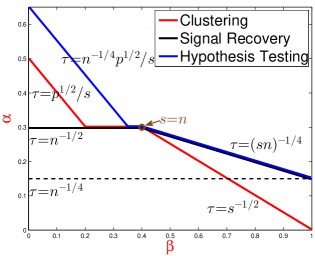
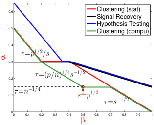
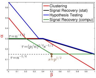
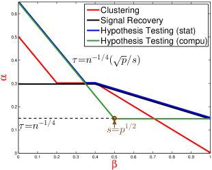
Figure 2: Top left: statistical limits for clustering (red), signal recovery (black), and hypothesis testing (blue); $s=p\epsilon_{p}$. Other three panels: CTUB for clustering (top right), signal recovery (bottom left) and hypothesis testing (bottom right), respectively (the three statistical limits in the top left panel are also shown for comparison).

1.7 Practical relevance and a real data example

The relatively idealized model we use allows very delicate analysis, but also raises practical concerns. In this section, we investigate IF-PCA with a real data example and illustrate that many ideas in previous sections are relevant in much broader settings.

Table 2: The clustering errors for Leukemia data with different numbers of selected features. Rows highlighted correspond to the threshold choices that yield lowest clustering errors.

$\#${selected features}	Errors	$\#${selected features}	Errors	$\#${selected features}	Errors
1	34	1419	3	2847	5
347	8	1776	1	3204	7
704	6	2133	1	3561	11
1062	5	2490	1

We use the leukemia data set on gene microarrays. This data set was cleaned by Dettling [17], consisting of $p=3571$ measured genes for $n=72$ samples from two classes: 47 from ALL (acute lymphoblastic leukemia), and 25 from AML (acute myeloid leukemia). The data set is available at www.stat.cmu.edu/~jiashun/Research/software/GenomicsData/ALL.

To implement IF-PCA, one noteworthy difficulty is the heteroscedasticity across genes in the data set. We apply IF-PCA with small modifications. In detail, arrange the data matrix as $X=[x_{1},\ldots,x_{p}]$ as before. Let $\bar{x}(j)=(1/n)\sum_{i=1}^{n}x_{j}(i)$, $m(x_{j})=\mathrm{median}(x_{j})$ and $d(j)=\mathrm{median}\{|x_{j}(1)-m(x_{j})|,\cdots,|x_{j}(n)-m(x_{j})|\}$ be the Median Absolute Deviation (MAD). We normalize by $x_{j}^{*}(i)=0.6745\cdot(x_{j}(i)-\bar{x}(j))/d(j)$, $1\leq i\leq n,1\leq j\leq p$. For $q>0$ to be determined, we select feature $j$ if and only if $(2n)^{-1}|\|x_{j}^{*}\|^{2}-n|>\sqrt{2q\log(p)}$. We then obtain the leading left singular vector $(\xi^{*})^{(q)}$ of the post-selection data matrix $[x_{1}^{*},\cdots,x_{p}^{*}]$ and cluster by applying the standard $k$-means algorithm to the leading eigenvector. In the last step, we can also cluster by the sign vector of $(\xi^{*})^{(q)}$ and the results are similar. The $k$-means algorithm has a slightly better performance.

Table 2 displays the clustering errors for different numbers of selected features (each corresponds to a choice of $q$). The table suggests that IF-PCA works nicely, with an error rate as low as $1/72$, if $q$ is set appropriately.

Figure 3 compares $(\xi^{*})^{(q)}$ for three choices of $q$: (a) the $q$ determined by applying the FDR controlling procedure [8] with the FDR parameter of $.05$ and simulated $P$-values under the null $x_{j}\sim N(0,I_{n})$, (b) the $q$ associated with the ideal number of selected features (see Table 2), and (c) the $q$ corresponding to classical PCA (any $q$ that allows us to skip the feature selection step works). This suggests that IF-PCA works well if $q$ is properly set.

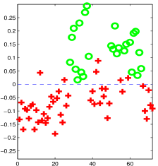
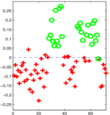
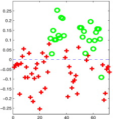
Figure 3: Leading left singular vector of the data matrix $X$ with very few features selected by FDR choice (left; 931 features chosen), with ideal number of features selected (middle; 2133 features chosen), and without feature selection (right). $y$-axis: entries of the left singular vector, $x$-axis: sample indices. Plots are based on Leukemia data, where red and green dots represent samples from the two classes ALL and AML, respectively.

We compare IF-PCA with classical methods of $k$-means and hierarchical clustering [25], $k$-means++ (a recent revision of the classical $k$-means; [6]), SpectralGem (classical PCA applied to $X^{*}$; [35]), and sparse $k$-means (a modification of $k$-means with sparse feature weights in the objective; [49]). The error rates are in Table 3, suggesting IF-PCA is effective in this case.

Table 3: Comparison of clustering errors (Leukemia data). Columns 2–7: numerator is the number of clustering errors, and denominator is the number of subjects.

Method	$k$-means	$k$-means++	Hierarchical	SpectralGem	Sparse $k$-means	IF-PCA
Error Rate	20/72	18.5/72	20/72	21/72	20/72	1/72

1.8 Comparison to works on the spike model

In our model (1.1)-(1.2), if we replace the Bernoulli model for $\ell_{i}$ in (1.1) by a Gaussian model where $\ell_{i}\stackrel{{\scriptstyle iid}}{{\sim}}N(0,\sigma^{2})$, then it becomes the spike model (Johnstone and Lu [32]).

In the spike model, while $\ell_{i}$’s are also of interest, the feature vector $\mu$ captures most of the attention: most recent works on the spike model (e.g., [4, 36, 47]) have been focused on signal recovery (and especially, sparse PCA). The two problems, signal recovery and clustering, are different. There are parameter settings where successful clustering is possible but successful signal recovery is impossible, and there are settings where the opposite is true; see Sections 1.4 and 1.6. Therefore, a direct extension of sparse PCA methods to clustering does not always work well.

Our work is also different from existing works on the spike model in terms of motivation and validation. Our model is motivated by cancer (subject) clustering, where the class labels $\ell_{i}$’s can be conveniently validated in many applications (e.g., see Section 1.7). In contrast, it is not easy to find real data sets where the feature vector $\mu$ is known, so it is comparably harder to validate the methods/theory on signal recovery or sparse PCA. Given the growing awareness of reproducibility and replicability [23], it becomes increasingly more important to develop methods and theory that can be directly validated by real applications. In a sense, our model extends the spike model to a new direction, and it helps strengthen (we hope) the ties between the recent theoretical interests on the spike model with real applications.

1.9 Content and notations

Section 2 studies the phase transition of IF-PCA, where we prove Theorem 1.4. Section 3 studies the statistical limits for signal recovery, where we prove Theorems 1.2, 1.3, 1.6, as well as Theorems 3.2-3.3 (to be introduced). Section 4 studies the statistical limits for hypothesis testing, where we prove Theorems 4.2-4.3 (to be introduced). Section 5 studies the lower bounds for all three problems and proves Theorems 1.1 and 1.5, as well as Theorems 3.1 and 4.1 (to be introduced). Other proofs are in the Appendix. Section 6 is for discussion.

In this paper, $L_{p}>0$ denotes a generic multi-$\log(p)$ term; see Section 1.5. When $\xi$ is a vector, $\|\xi\|_{q}$ denotes the vector $L^{q}$-norm, $0\leq q\leq\infty$ (the subscript is dropped for simplicity if $q=2$). When $\xi$ is a matrix, $\|\xi\|$ denotes the matrix spectral norm, and $\|\xi\|_{F}$ denotes the matrix Frobenius norm. For two vectors $\xi,\eta$, $\langle\xi,\eta\rangle$ denotes the inner product of them, and $\mathrm{cos}(\xi,\eta)=|\langle\xi/\|\xi\|,\eta/\|\eta\|\rangle|$. For any two probability densities $f$ and $g$, $\|f-g\|_{1}$ and $H(f,g)$ are the $L^{1}$-distance and the Hellinger distance, respectively. For any real value $a$, $\lceil a\rceil$ is the smallest integer that is no smaller than $a$. We say two positive sequences $a_{n}\sim b_{n}$, $a_{n}\lesssim b_{n}$ and $a_{n}\gtrsim b_{n}$ if $\lim_{n\rightarrow\infty}a_{n}/b_{n}=1$, $\lim\sup_{n\rightarrow\infty}a_{n}/b_{n}\leq 1$ and $\lim\inf_{n\rightarrow\infty}a_{n}/b_{n}\geq 1$, respectively. For two sets $A,B$, $A\Delta B=(A\backslash B)\cup(B\backslash A)$.

2 Phase transition for IF-PCA

In this section, we prove Theorem 1.4. Our proofs need very precise characterization of the spectra of the post-selection Gram matrix $X^{(q)}(X^{(q)})^{\prime}$. Specifically, we need both a tight upper bound on the range of the spectra of $X^{(q)}(X^{(q)})^{\prime}$ (Lemma 2.1) and a tight lower bound for the largest eigenvalue of $X^{(q)}(X^{(q)})^{\prime}$ (Lemma 2.2). The main challenges are that, due to feature selection,

• the entries of $X^{(q)}$ are no longer independent,

• the conditional distribution of each survived column is unclear.

For this reason, existing results on RMT do not apply directly and we need to develop new theory on post-selection RMT. Our analysis adapts that in Vershynin [45] and uses the results of covering number in Rogers [40].

Remark. For the spike model, there are results about the spectra of a different post-selection Gram matrix $(X^{(q)})^{\prime}X^{(q)}$ (e.g., Thereom 2 of [32]). Since feature selection is column-wise, the leading eigenvectors of $(X^{(q)})^{\prime}X^{(q)}$ and $X^{(q)}(X^{(q)})^{\prime}$ have very different behaviors. Moreover, the settings of [32, Theorem 2] implicitly force $X^{(q)}$ to have much more rows than columns (which we call the “skinny” case), but our results do not have such a restriction.

To show the claim, it suffices to show the claim for any fixed realization of $(\ell,\mu)$ in the event

$$D_{p}=\{\mu:\bigl{|}|S(\mu)|-p\epsilon_{p}\bigr{|}\leq\sqrt{6p\epsilon_{p}\log(p)}\};$$

note that $P(D_{p}^{c})=O(p^{-3})$ and the event only has a negligible effect. Fixing $0<q<1$ and a realization of $(\ell,\mu)$ in $D_{p}$. Let $\hat{S}_{q}^{(if)}(\ell,\mu)$ be the set of all survived features. In our model, $X=\ell\mu^{\prime}+Z$, and $Z=[z_{1},z_{2},\ldots,z_{p}]$. Introduce a vector $\mu^{(q)}=\mu^{(q)}(\ell,\mu)\in R^{p}$ and a matrix $Z^{(q)}=[z_{1}^{(q)},\cdots,z_{p}^{(q)}]\in R^{n,p}$ by

$$\mu^{(q)}(j)=\mu(j)\cdot 1\{j\in\hat{S}^{(if)}_{q}(\ell,\mu)\},\;\;z_{j}^{(q)}=z_{j}\cdot 1\{j\in\hat{S}^{(if)}_{q}(\ell,\mu)\},\;\;1\leq j\leq p,$$

and so the post-selection data matrix $X^{(q)}=X^{(q)}(\ell,\mu)$, viewed as an $n\times p$ matrix with many zero columns, satisfies

$$X^{(q)}(\ell,\mu)=\ell\mu^{(q)}(\ell,\mu)+Z^{(q)}(\ell,\mu).$$

Fixing $(\beta,\theta,r)\in(0,1)^{3}$ and $q>0$, and assuming $z\sim N(0,I_{n})$, introduce $m^{(q)}_{0}(\mu)=(p-|S(\mu)|)\cdot P(\|z\|^{2}>n+2\sqrt{qn\log(p)})$, $m^{(q)}_{1}(\ell,\mu)=|S(\mu)|\cdot P(\|z+\tau_{p}^{*}\ell\|^{2}>n+2\sqrt{qn\log(p)})$, and $m^{(q)}(\ell,\mu)=m_{0}^{(q)}(\ell,\mu)+m_{1}^{(q)}(\ell,\mu)$. Note that $m_{0}^{(q)}(\ell,\mu)$ and $m_{1}^{(q)}(\ell,\mu)$ are the expected numbers of survived useless/useful features, respectively. We also need the following counterpart of $m^{(q)}(\ell,\mu)$:

$$m_{*}^{(q)} (\ell,\mu)=(p-|S(\mu)|)\cdot n^{-1}E\big{(}\|z\|^{2}1\{\|z\|^{2}>n+2\sqrt{qn\log(p)}\}\big{)}$$

$$+|S(\mu)|\cdot n^{-1}E\big{(}\|z\|^{2}1\{\|z+\tau_{p}^{*}\ell\|^{2}>n+2\sqrt{qn\log(p)}\}\big{)}.$$

The dependence on $(\ell,\mu)$ is tedious, so for notational simplicity, we may drop them without further notices.

The term $m^{(q)}$ is the expected number of selected features, and plays an important role. By tail properties of chi-square distributions (see Section B.1), with probability $1-O(p^{-3})$,

$$m_{*}^{(q)}\sim m^{(q)}\sim L_{p}[p^{1-q}+p\epsilon_{p}p^{-[(\sqrt{q}-\sqrt{r})_{+}]^{2}}],$$ (2.1)

where as before $L_{p}$ is a generic multi-$\log(p)$ term. Recalling $n=p^{\theta}$, define

$$\tilde{q}(\beta,\theta,r)=\left\{\begin{array}[]{lr}\max\{1-\theta,(\sqrt{1-\beta-\theta}+\sqrt{r})^{2}\},&\beta<1-\theta,\\ 1-\theta,&\beta>1-\theta.\end{array}\right.$$

By (2.1) and basic algebra, it is seen that there are two different cases:

• (“Fat”). When $q<\tilde{q}(\beta,\theta,r)$, $m^{(q)}/n\rightarrow\infty$ and $X^{(q)}$ has much more columns than rows.

• (“Skinny”). When $q>\tilde{q}(\beta,\theta,r)$, $m^{(q)}/n\rightarrow 0$ and $X^{(q)}$ has much more rows than columns.

Lemma 2.1

(Upper bound for the range of eigenvalues of $Z^{(q)}(Z^{(q)})^{\prime}$). Suppose conditions of Theorem 1.4 hold. There exists a universal constant $C>0$ such that for any fixed $q>0$, as $p\rightarrow\infty$, conditioning on any realization of $(\ell,\mu)$ from the event $D_{p}$, with probability at least $1-O(p^{-3})$,

• (“Fat” case). When $q<\tilde{q}(\beta,\theta,r)$, all eigenvalues of $Z^{(q)}(Z^{(q)})^{\prime}$ fall between $m^{(q)}_{*}\pm[C\sqrt{nm^{(q)}\log(p)}+o(m_{1}^{(q)})]$.

• (“Skinny” case). When $q>\tilde{q}(\beta,\theta,r)$, all nonzero eigenvalues of $Z^{(q)}(Z^{(q)})^{\prime}$ fall between $n\pm C\sqrt{nm^{(q)}\log(p)}$.

Remark. Noting that $m^{(q)}$ is the expected number of columns of $Z^{(q)}$, our results are very similar to the well-known results on eigenvalues of RMT in the case where we have an $n\times m^{(q)}$ matrix with $iid$ $N(0,1)$ entries. However, we need more sophisticated proofs, as the rows of $Z^{(q)}$ are dependent and the distribution of the columns of $Z^{(q)}$ is unknown and hard to characterize.

For the “fat” case, it turns out that Lemma 2.1 is insufficient: we need both an improved upper bound on the range (with the $\sqrt{\log(p)}$ factor eliminated) and a lower bound on the leading eigenvalue.

Lemma 2.2

(Improved bound (“fat” case)). Suppose the conditions of Theorem 1.4 hold and $r<\rho^{*}_{\theta}(\beta)$. There exist constants $c_{1}>c_{2}>0$ such that as $p\to\infty$, for any fixed $q>0$, conditioning on any realization of $(\ell,\mu)$ from the event $D_{p}$, with probability $1-O(n^{-2})$,

• All singular values of $Z^{(q)}(Z^{(q)})^{\prime}$ fall between $m^{(q)}_{*}\pm c_{1}\sqrt{nm^{(q)}}$;

• $\lambda_{\max}(Z^{(q)}(Z^{(q)})^{\prime})\geq m_{*}^{(q)}+c_{2}\sqrt{nm^{(q)}}$.

We now prove Theorem 1.4. We show the cases of $r>\rho^{*}_{\theta}(\beta)$ (Region of Possibility) and $r<\rho^{*}_{\theta}(\beta)$ (Region of Impossibility) separately.

2.1 Region of Possibility

Consider the case $r>\rho_{\theta}^{*}(\beta)$. Recall that

$$q=q^{*}(\beta,\theta,r)=\left\{\begin{array}[]{ll}4r,&r<(\beta-\theta/2)/3,\\ \frac{(\beta-\theta/2+r)^{2}}{4r},&(\beta-\theta/2)/3\leq r<1.\end{array}\right.$$

Let $\xi^{*}$ be the first left singular vector of $X^{(q)}$ at $q=q^{*}(\beta,\theta,r)$. The goal is to show

$$\mathrm{cos}(\ell,\xi^{*})\rightarrow 1.$$

Write

$$X^{(q)}(X^{(q)})^{\prime}=\|\mu^{(q)}\|^{2}\ell\ell^{\prime}+Z^{(q)}(Z^{(q)})^{\prime}+A,$$ (2.2)

where $A=\ell(\mu^{(q)})^{\prime}(Z^{(q)})^{\prime}+Z^{(q)}\mu^{(q)}\ell^{\prime}$ for short. On the right hand side of (2.2), the first matrix has a rank $1$, with $n\|\mu^{(q)}\|^{2}$ being the only nonzero eigenvalue and $\ell$ being the associated eigenvector. In our model, the expectation of $\|\mu^{(q)}\|^{2}$ is equal to $(\tau_{p}^{*})^{2}m_{1}^{(q)}$, where by tail properties of chi-square distributions (see Section B.1), $m_{1}^{(q)}=L_{p}p^{1-\beta}p^{-[(\sqrt{q}-\sqrt{r})_{+}]^{2}}$ with overwhelming probabilities. It follows that with a probability at least $1-O(p^{-3})$,

$$n\|\mu^{(q)}\|^{2}\gtrsim n(\tau_{p}^{*})^{2}\cdot m_{1}^{(q)}\sim L_{p}p^{\Delta(q,\beta,\theta,r)},$$

where $\Delta(q,\beta,\theta,r)=1+\theta/2-\beta-[(\sqrt{q}-\sqrt{r})_{+}]^{2}$. Compare this with (2.2). By perturbation theory in matrices [11, 16], to show the claim, it suffices to show that there is a scalar $a^{*}$ (either random or non-random) and a constant $\delta^{*}>0$ so that

$$\|Z^{(q)}(Z^{(q)})^{\prime}+A-a^{*}I_{n}\|\leq L_{p}p^{\Delta(q,\beta,\theta,r)-\delta^{*}}.$$

To this end, note that by triangle inequality,

$$\|Z^{(q)}(Z^{(q)})^{\prime}+A-a^{*}I_{n}\|\leq\|Z^{(q)}(Z^{(q)})^{\prime}-a^{*}I_{n}\|+\|A\|.$$

The following lemma is proved in the Appendix.

Lemma 2.3

Suppose conditions of Theorem 1.4 hold. For any fixed $q>0$, as $p\rightarrow\infty$, conditioning on any realization of $(\ell,\mu)$ from the event $D_{p}$, with probability $1-O(p^{-3})$, $\|\ell(\mu^{(q)})^{\prime}(Z^{(q)})^{\prime}+Z^{(q)}\mu^{(q)}\ell^{\prime}\|\leq Cn\tau_{p}^{*}\sqrt{m_{1}^{(q)}}$.

The key to the proof is to control $\|Z^{(q)}\mu^{(q)}\|_{\infty}$ using the Bernstein inequality [41] and to study the distribution of $Z^{(q)}$. See [29] for details.

Now, when $q>\tilde{q}(\beta,\theta,r)$, we are in the “skinny” case, combining Lemmas 2.1 and 2.3, we have that with probability at least $1-O(p^{-3})$,

$$\|Z^{(q)}(Z^{(q)})^{\prime}+A\|\lesssim n+C\Big{(}n\tau_{p}^{*}\sqrt{m_{1}^{(q)}}+\sqrt{nm^{(q)}\log(p)}\Big{)}\leq L_{p}p^{\frac{\theta}{2}+\frac{1}{2}\max\{\theta,\Delta(q,\beta,\theta,r)\}}.$$

In the last inequality, we have used (2.1) which indicates that $m_{0}^{(q)}=L_{p}p^{1-q}$ and $m_{1}^{(q)}=L_{p}p^{1-\beta-[(\sqrt{q}-\sqrt{r})_{+}]^{2}}$. By the condition of $r>\rho_{\theta}^{*}(\beta)$, it can be shown that $\Delta(q,\beta,\theta,r)>\theta$, and the claim follows by letting $a^{*}=0$ and $\delta^{*}=\frac{\Delta-\theta}{2}$. When $q<\tilde{q}(\beta,\theta,r)$, we are in the “fat” case. Combining Lemmas 2.1 and 2.3, with probability at least $1-O(p^{-3})$,

$$\|Z^{(q)}(Z^{(q)})^{\prime}+A-m_{*}^{(q)}I_{n}\| \leq C\Big{(}n\tau_{p}^{*}\sqrt{m_{1}^{(q)}}+\sqrt{nm^{(q)}\log(p)}+n^{-1}m_{1}^{(q)}\Big{)}$$

$$\leq L_{p}p^{\frac{\theta}{2}+\frac{1}{2}\max\{\theta,\Delta(q,\beta,\theta,r),1-q\}}+p^{\Delta(q,\beta,\theta,r)-\frac{3\theta}{2}}.$$

By the condition of $r>\rho^{*}_{\theta}(\beta)$, it can be shown that $\Delta(q,\beta,\theta,r)>\max\{\theta,\frac{\theta+1-q}{2}\}$, and the claim follows by letting $a^{*}=m_{*}^{(q)}$ and $\delta^{*}=\min\{\frac{\Delta-\theta}{2},\Delta-\frac{1-q+\theta}{2},\frac{3\theta}{2}\}$.

2.2 Region of Impossibility

Consider the case $r<\rho^{*}_{\theta}(\beta)$. Fix $0<q<1$. Recall that $\xi^{(q)}$ is first left singular vector of $X^{(q)}$. The goal is to show that

$$\mathrm{cos}(\ell,\xi^{(q)})\leq c_{0}<1,\qquad\mbox{for any }0<q<1,$$ (2.3)

where $c_{0}$ is a universal constant independent of $q$. Denote for short $H=X^{(q)}(X^{(q)})^{\prime}$, $H_{0}=Z^{(q)}(Z^{(q)})^{\prime}$, $\xi=\xi^{(q)}$, and $\tilde{\ell}=\ell/\|\ell\|$. Let the eigenvalues of $H$ be $\lambda_{1}(H)\geq\lambda_{2}(H)\geq\ldots\geq\lambda_{n}(H)$. Write

$$\tilde{\ell}=a\xi+\sqrt{1-a^{2}}\eta,\qquad\mbox{for a unit-norm vector $\eta$ such that $\eta\perp\xi$}.$$

Note that $\xi^{\prime}H\eta=\lambda_{1}\xi^{\prime}\eta=0$ and $\eta^{\prime}H\eta\geq\lambda_{n}$, we have $\tilde{\ell}^{\prime}H\tilde{\ell}=a^{2}\xi^{\prime}H\xi+2a\sqrt{1-a^{2}}\xi^{\prime}H\eta+(1-a^{2})\eta^{\prime}H\eta\geq a^{2}\lambda_{1}+(1-a^{2})\lambda_{n}$. Rearranging it gives $a^{2}\leq 1-[\lambda_{1}(H)-\tilde{\ell}^{\prime}H\tilde{\ell}]/[\lambda_{1}(H)-\lambda_{n}(H)]$. Note that $\mathrm{cos}(\ell,\xi)=|a|$. So to show (2.3), it suffices to show there

$$\frac{\lambda_{1}(H)-\tilde{\ell}^{\prime}H\tilde{\ell}}{\lambda_{1}(H)-\lambda_{n}(H)}\geq 1-c_{0}^{2},\qquad\mbox{for some constant $c_{0}\in(0,1)$}.$$ (2.4)

The following lemma is proved in the Appendix.

Lemma 2.4

Suppose $r<\rho^{*}_{\theta}(\beta)$ and the conditions of Theorem 1.4 hold. As $p\to\infty$, for any fixed $q>0$, conditioning on any realization of $(\ell,\mu)$ from the event $D_{p}$, for any $v\in\mathcal{S}^{n-1}$, with probability $1-O(p^{-3})$, $|v^{\prime}H_{0}v-m_{*}^{(q)}|\leq C\sqrt{m^{(q)}\log(p)}$, and

$$\|H-H_{0}\|=\left\{\begin{array}[]{ll}o(n),&\qquad\mbox{$q>\tilde{q}(\beta,r,\theta)$ (``skinny" case)},\\ o(\sqrt{nm^{(q)}}),&\qquad\mbox{$q<\tilde{q}(\beta,r,\theta)$ (``fat" case)}.\end{array}\right.$$ (2.5)

We now show (2.4). Similarly, let $\lambda_{1}(H_{0})\geq\lambda_{2}(H_{0})\geq\ldots\geq\lambda_{n}(H_{0})$ be the eigenvalues of $H_{0}$. We prove for the cases of $q>\tilde{q}(\beta,r,\theta)$ and $q<\tilde{q}(\beta,r,\theta)$ separately. Consider the first case. This is the “skinny” case where $m^{(q)}\ll n$. By Lemma 2.1 and the first claim of Lemma 2.4, with probability $1-O(p^{-3})$, $\lambda_{1}(H_{0})\sim n$, $\lambda_{n}(H_{0})\geq 0$ and $\tilde{\ell}^{\prime}H_{0}\tilde{\ell}=o(n)$. By the second claim of Lemma 2.4, $\|H-H_{0}\|=o(n)$. Combining the above with Weyl’s inequality [48] (i.e., $\max_{1\leq i\leq n}|\lambda_{i}(H)-\lambda_{i}(H_{0})|\leq\|H-H_{0}\|$), we have

$$\lambda_{1}(H)-\lambda_{n}(H)\leq n+o(n),\qquad\lambda_{1}(H)-\tilde{\ell}^{\prime}H\tilde{\ell}\geq n-o(n).$$

Inserting these into (2.4) gives the claim.

Consider the second case. This is the “fat” case and $m^{(q)}\gg n$. By Lemma 2.2 and the first claim of Lemma 2.4, there is $\lambda_{1}(H_{0})-\lambda_{n}(H_{0})\leq c_{2}\sqrt{nm^{(q)}}$ and $\lambda_{1}(H_{0})-\tilde{\ell}^{\prime}H_{0}\tilde{\ell}\gtrsim c_{1}\sqrt{nm^{(q)}}$. Similarly, combining these with the second claim of Lemma 2.4 and Weyl’s inequality, we find that

$$\lambda_{1}(H)-\lambda_{n}(H)\lesssim c_{2}\sqrt{nm^{(q)}},\qquad\lambda_{1}(H)-\tilde{\ell}^{\prime}H\tilde{\ell}\gtrsim c_{1}\sqrt{nm^{(q)}}.$$

Inserting these into (2.4) gives the claim.

3 Limits for signal recovery

In this section, we discuss limits for signal (support) recovery. The results are intertwined with those for clustering (namely, Theorems 1.1-1.3 and Theorem 1.5), so we prove all of them together in the later part of the section.

Compare two problems: signal recovery and clustering. One useful insight is that in the less sparse case, clustering is comparably easier than signal recovery, so we should estimate $\ell$ first and then use it to estimate $S(\mu)$; in the more sparse case, we should do the opposite.

For the less sparse case, we have introduced two clustering methods, $\hat{\ell}_{*}^{(sa)}$ and $\hat{\ell}_{*}^{(if)}$, in Section 1.1. They give rise to two signal recovery methods, $\hat{S}_{*}^{(sa)}$ and $\hat{S}_{*}^{(if)}$. In detail, let $y_{*}^{(sa)}=n^{-1/2}X^{\prime}\hat{\ell}_{*}^{(sa)}$ and $y_{*}^{(if)}=n^{-1/2}X^{\prime}\hat{\ell}_{*}^{(if)}$, and let $t_{p}^{*}=\sqrt{2\log(p)}$ be the universal threshold [22]. Respectively, $\hat{S}_{*}^{(sa)}$ and $\hat{S}_{*}^{(if)}$ are defined by

$$\hat{S}_{*}^{(sa)}=\{1\leq j\leq p:|y_{*,j}^{(sa)}|\geq t_{p}^{*}\},\qquad\hat{S}_{*}^{(if)}=\{1\leq j\leq p:|y_{*,j}^{(if)}|\geq t_{p}^{*}\}.$$

For the more sparse case, we introduce two methods $\hat{S}_{N}^{(sa)}$ and $\hat{S}_{q}^{(if)}$; they are in fact the ones that give rise to the clustering methods $\hat{\ell}_{N}^{(sa)}$ and $\hat{\ell}_{q}^{(if)}$ we introduced in Section 1.1. In detail, recalling that $Q(j)=(2n)^{-1/2}(\|x_{j}\|^{2}-n)$ is the column-wise $\chi^{2}$-statistics,

$$\hat{S}_{N}^{(sa)}=\mathrm{argmax}_{\{S:S\subset\{1,2,\ldots,p\},|S|=N\}}\{N^{-1/2}\|\sum\nolimits_{j\in S}x_{j}\|_{1}\},$$ (3.1)

and

$$\hat{S}_{q}^{(if)}=\{1\leq j\leq p:Q(j)\geq\sqrt{2q\log(p)}\}.$$

For any signal (support) recovery procedure $\hat{S}$, we measure the performance by the normalized size of the difference of $\hat{S}$ and the true support

$$\mathrm{Hamm}_{p}(\hat{S},\alpha,\beta,\theta)=(p\epsilon_{p})^{-1}E(|\hat{S}\Delta S(\mu)|),$$ (3.2)

where $A\Delta B=(A\setminus B)\cup(B\setminus A)$ denotes the symmetric difference of two sets and the expectation is with respective to the randomness of $(\mu,\ell,Z)$. If we think $\hat{S}$ as an estimate of $\mu$, say, $\hat{\mu}$, and $E(|\hat{S}\Delta S(\mu)|)$ is actually the Hamming distance between the two vectors $(\hbox{\rm sgn}(|\hat{\mu}(1)|),\ldots,\hbox{\rm sgn}(|\hat{\mu}(p)|))^{\prime}$ and $(\hbox{\rm sgn}(\mu(1)),\ldots,\hbox{\rm sgn}(\mu(p)))^{\prime}$. For this reason, we call that in (3.2) the (normalized) Hamming distance.

In Section 1.6, we have introduced the curves $\alpha=\eta^{sig}_{\theta}(\beta)$ and $\alpha=\tilde{\eta}^{sig}_{\theta}(\beta)$. The following theorem is proved in Section 5.

Theorem 3.1

(Statistical lower bound for signal recovery). Fix $(\alpha,\beta,\theta)\in(0,1)^{3}$ and suppose $\alpha>\eta_{\theta}^{sig}(\beta)$. Consider the signal recovery problem for Models (1.1)-(1.2) and (1.7)-(1.8). For any $\hat{S}$ that is an estimate for the support of $S$, $\mathrm{Hamm}_{p}(\hat{S},\alpha,\beta,\theta)\gtrsim 1$ as $p\rightarrow\infty$.

We also have the following theorems, which are proved below.

Theorem 3.2

(Statistical upper bound for signal recovery). Fix $(\alpha,\beta,\theta)\in(0,1)^{3}$ and suppose $\alpha<\eta_{\theta}^{sig}(\beta)$. Consider the signal recovery problem for Models (1.1)-(1.2) and (1.7)-(1.8). As $p\rightarrow\infty$,

• $\mathrm{Hamm}_{p}(\hat{S}_{*}^{(sa)},\alpha,\beta,\theta)\rightarrow 0$, if $0<\beta<(1-\theta)/2$.

• $\mathrm{Hamm}_{p}(\hat{S}_{N}^{(sa)},\alpha,\beta,\theta)\rightarrow 0$, if $(1-\theta)/2<\beta<1$ and $N=\lceil p\epsilon_{p}\rceil$.

Theorem 3.3

(CTUB for signal recovery). Fix $(\alpha,\beta,\theta)\in(0,1)^{3}$ and suppose $\alpha<\tilde{\eta}_{\theta}^{sig}(\beta)$. Consider the signal recovery problem for Models (1.1)-(1.2) and (1.7)-(1.8). As $p\rightarrow\infty$,

• $\mathrm{Hamm}_{p}(\hat{S}_{*}^{(sa)},\alpha,\beta,\theta)\rightarrow 0$, if $0<\beta<(1-\theta)/2$.

• $\mathrm{Hamm}_{p}(\hat{S}_{*}^{(if)},\alpha,\beta,\theta)\rightarrow 0$, if $(1-\theta)/2<\beta<1/2$.

• $\mathrm{Hamm}_{p}(\hat{S}_{q}^{(if)},\alpha,\beta,\theta)\rightarrow 0$, if $(1-\theta)/2<\beta<1/2$ and $q\geq 3$.

3.1 Proofs of Theorems 1.2-1.3, 1.6 and 3.2-3.3

We need two lemmas. The first one is on classical PCA, and it is needed for studying $\hat{\ell}_{*}^{(if)}$ and $\hat{S}_{*}^{(if)}$. The second one is a large-deviation inequality for folded normal random variables and it is needed for studying the optimization problem in (3.1).

Lemma 3.1

Fix $(\alpha,\beta,\theta)\in(0,1)^{3}$ such that $(1-\theta)/2<\beta<1/2$ and $\alpha<\tilde{\eta}_{\theta}^{clu}(\beta)$. In Models (1.1)-(1.2) and (1.7)-(1.8), let $\lambda$ be the first eigenvalue of $XX^{\prime}$ and $\xi$ be the corresponding eigenvector. There is a generic constant $\delta=\delta(\alpha,\beta,\theta)>0$ such that with probability $1-O(p^{-3})$,

$$\min\{\|\sqrt{n}\xi+\ell\|_{\infty},\|\sqrt{n}\xi-\ell\|_{\infty}\}<p^{-\delta}.$$

The claim continues to hold if we replace the model (1.2) by (1.15) for $A=I_{n}$ and $B$ such that $\max\{\|B\|,\|B^{-1}\|\}\leq L_{p}$.

Lemma 3.2

(Large-deviation on Folded Normals). As $n\rightarrow\infty$, for any $h>0$ and $0\leq x\leq\sqrt{n}/\log(n)$, and $n$ independent samples $z_{i}$ from $N(0,1)$,

$$P\bigl{(}\bigl{|}\sum\nolimits_{i=1}^{n}\bigl{(}|z_{i}+h|-E[|z_{i}+h|]\bigr{)}\bigr{|}\geq\sqrt{n}x\bigr{)}\leq 2\mathrm{exp}\bigl{(}-(1+o(1))x^{2}/2\bigr{)},$$

where $o(1)\rightarrow 0$, uniformly for all $h>0$ and $0<x\leq\sqrt{n}/\log(n)$.

We now show all theorems about upper bound. Since Theorems 1.2-1.3 are special cases of Theorem 1.6 with $B=I_{p}$, it suffices to show Theorems 1.6 and 3.2-3.3. As there are four methods involved, it is more convenient to prove in a way by grouping the items associated with each method together. Fixing $(\alpha,\beta,\theta)\in(0,1)^{3}$ and viewing all statements in Theorems 1.6 and Theorems 3.2-3.3, what we need to show can be re-organized as follows (for the statements regarding $\hat{\ell}$, we need to prove that they hold for a general B where $\max\{\|B\|,\|B^{-1}\|\}\leq L_{p}$).

• (a). Simple Aggregation. Consider the case $0<\beta<(1-\theta)/2$. In this range, $\eta_{\theta}^{sig}(\beta)<\eta_{\theta}^{clu}(\beta)$. All we need to show is that if $\alpha<\eta_{\theta}^{clu}(\beta)$, then $\hat{\ell}_{*}^{(sa)}=\ell$ with probability at least $1-O(p^{-3})$, and that if additionally $\alpha<\eta_{\theta}^{sig}(\beta)$, then $\mathrm{Hamm}_{p}(\hat{S}_{*}^{(sa)},\alpha,\beta,\theta)\rightarrow 0$.

• (b). Sparse Aggregation. Consider the case $(1-\theta)/2<\beta<1$. In this case, $\eta_{\theta}^{clu}(\beta)\leq\eta_{\theta}^{sig}(\beta)$. Letting $N=\lceil p\epsilon_{p}\rceil$, all we need to show is that $\mathrm{Hamm}_{p}(\hat{S}_{N}^{(sa)},\alpha,\beta,\theta)\rightarrow 0$ if $\alpha<\eta_{\theta}^{sig}(\beta)$ and $\mathrm{Hamm}_{p}(\hat{\ell}_{N}^{(sa)},\alpha,\beta,\theta)\rightarrow 0$ if additionally $\alpha<\eta_{\theta}^{clu}(\beta)$.

• (c). Classical PCA. Consider the case $(1-\theta)/2<\beta<1/2$ where only computationally tractable bounds are concerned and $\tilde{\eta}^{clu}_{\theta}(\beta)=\tilde{\eta}_{\theta}^{sig}(\beta)$. All we need to show is that if $\alpha<\tilde{\eta}_{\theta}^{clu}(\beta)$, then $\hat{\ell}_{*}^{(if)}=\pm\ell$ with probability at least $1-O(p^{-3})$ and that $\mathrm{Hamm}_{p}(\hat{S}_{*}^{(if)},\alpha,\beta,\theta)\rightarrow 0$.

• (d). IF-PCA. Consider the case $1/2<\beta<1$ where only computationally tractable bounds are concerned and $\tilde{\eta}_{\theta}^{clu}(\beta)\leq\tilde{\eta}_{\theta}^{sig}(\beta)$. All we need to show is that if $\alpha<\tilde{\eta}_{\theta}^{sig}(\beta)$, then $\hat{S}_{q}^{(if)}=S(\mu)$ with probability at least $1-O(p^{-3})$; and if additionally $\alpha<\tilde{\eta}_{\theta}^{clu}(\beta)$, then $\mathrm{Hamm}_{p}(\hat{\ell}_{q}^{(if)},\alpha,\beta,\theta)\rightarrow 0$.

Consider (a). Note that $\hat{\ell}_{*}^{(sa)}=\mathrm{sgn}(\sum_{j=1}^{p}x_{j})$ and $\sum_{j=1}^{p}x_{j}\sim N(\|\mu\|_{0}\tau\ell,pI_{n})$. By (3.3), $\|\mu\|_{0}\tau=p^{1-\beta-\alpha}(1+o(1))$. Hence, $\alpha<\eta_{\theta}^{clu}(\beta)$ implies $\|\mu\|_{0}\tau\gg\sqrt{p}$, and it follows that $\hat{\ell}_{*}^{(sa)}=\ell$ with overwhelming probability. Once $\hat{\ell}_{*}^{(sa)}=\ell$, $y_{*}^{(sa)}=n^{-1/2}X^{\prime}\ell\sim N(\sqrt{n}\mu,I_{p})$. Noting that $\alpha<\eta^{sig}_{\theta}(\beta)$ implies $\sqrt{n}\tau\gg 1$, we have $\mathrm{Hamm}_{p}(\hat{S}_{*}^{(sa)})\rightarrow 0$ with overwhelming probability. Consider (c). The first claim is a direct result of Lemma 3.1, and the second claim can be proved similarly as in (a). Consider (d). Recall that the column-wise test statistic $Q(j)$ is approximately distributed as $N(0,1)$ for useless features and $N(\sqrt{n/2}\tau^{2},1)$ for useful features. So $\tau\gg n^{-1/4}$ will assure successful signal recovery, which translates to $\alpha<\tilde{\eta}_{\theta}^{sig}(\beta)$. Once $\hat{S}_{q}^{(if)}=S(\mu)$, we restrict our attention to $X^{S(\mu)}$, the sub-matrix of $X$ restricted to the columns in $S(\mu)$, and the claim of Lemma 3.1 continues to hold by adapting the proof there (see the Appendix for details). So $\mathrm{Hamm}_{p}(\hat{\ell}^{(if)}_{q})\rightarrow 0$ with overwhelming probability. It remains to prove (b).

We now show (b). Define $\hat{\mu}_{N}^{(sa)}$ such that $\hat{\mu}_{N}^{(sa)}(j)=\tau_{p}\cdot 1\{j\in\hat{S}_{N}^{(sa)}\}$. Write $\hat{S}_{N}^{(sa)}=\hat{S}$, $\hat{\mu}_{N}^{(sa)}=\hat{\mu}$, $\hat{\ell}^{(sa)}_{N}=\hat{\ell}$ and $s_{p}=p\epsilon_{p}$. With probability $1-O(p^{-3})$,

$$|\|\mu\|_{0}-s_{p}|\leq C\sqrt{s_{p}\log(p)}.$$ (3.3)

Since any event of probability $O(p^{-3})$ has a negligible effect to the Hamming distances, we always condition on a fixed realization $(\ell,\mu)$ that satisfy (3.3); so the probabilities below are with respective to the randomness of $Z$. To show (b), all we need to show are

• (b1). $\mathrm{Hamm}_{p}(\hat{\ell},\alpha,\beta,\theta)\rightarrow 0$, if $\alpha<\eta_{\theta}^{clu}(\beta)$. In this item, the matrix $B$ may be any matrix that satisfies $\max\{\|B\|,\|B^{-1}\|\}\leq L_{p}$.

• (b2). $\mathrm{Hamm}_{p}(\hat{S},\alpha,\beta,\theta)\rightarrow 0$, if $\alpha<\eta_{\theta}^{sig}(\beta)$. In this item, $B=I_{p}$.

Consider (b1) first. It suffices to show

$$n^{-1}\langle\hat{\ell},\ell\rangle\rightarrow 1.$$ (3.4)

For any realized $\mu$, we construct $\tilde{\mu}$ as follows:

• If $\|\mu\|_{0}>N$, replace $\|\mu\|_{0}-N$ nonzero entries by $0$.

• If $\|\mu\|_{0}<N$, replace $N-\|\mu\|_{0}$ zero entries by $\tau_{p}$.

Let $\tilde{S}$ be the support of $\tilde{\mu}$. Write $X\tilde{\mu}=\|B\tilde{\mu}\|\cdot[Z(B\tilde{\mu}/\|B\tilde{\mu}\|)+\langle\mu,\tilde{\mu}/\|B\tilde{\mu}\|\rangle\ell]$, where $Z(B\tilde{\mu}/\|B\tilde{\mu}\|)\sim N(0,I_{n})$ and $\langle\mu,\tilde{\mu}/\|B\tilde{\mu}\|\rangle\gtrsim\|B\|^{-1}\tau_{p}\sqrt{s_{p}}=L_{p}p^{(1-\beta-2\alpha)/2}$, with $(1-\beta-2\alpha)>0$ in our range of interest. According to Mills’ ratio [41], with probability $1-O(p^{-3})$, the absolute value of standard normal variable is bounded by $\sqrt{6\log(p)}$, which is less than $L_{p}p^{(1-\beta-2\alpha)/2}$ when $p\rightarrow\infty$. It follows that with probability at least $1-O(p^{-3})$, $\hbox{\rm sgn}(X\tilde{\mu})=\ell$. Furthermore, $\ell^{\prime}X\tilde{\mu}=\|X\tilde{\mu}\|_{1}=\tau_{p}\|\sum_{j\in\tilde{S}}x_{j}\|_{1}$. Since that $\hat{\ell}^{\prime}X\hat{\mu}=\|X\hat{\mu}\|_{1}=\tau_{p}\|\sum_{j\in\hat{S}}x_{j}\|_{1}$ and that $\hat{S}$ solves the optimization problem (3.1),

$$\hat{\ell}^{\prime}X\hat{\mu}\geq\ell^{\prime}X\tilde{\mu}.$$ (3.5)

Write $\hat{\ell}^{\prime}X\hat{\mu}=\langle\hat{\ell},\ell\rangle\langle\mu,\hat{\mu}\rangle+\hat{\ell}^{\prime}ZB\hat{\mu}$. We aim to obtain an upper bound for $|\hat{\ell}^{\prime}ZB\hat{\mu}|$ (an upper bound for $|\ell^{\prime}ZB\tilde{\mu}|$ can be obtained similarly). Denote by $(ZB)^{\hat{S}}$ the sub-matrix of $ZB$ containing columns in $\hat{S}$. Then $|\hat{\ell}^{\prime}ZB\hat{\mu}|\leq\sqrt{n}\|(ZB)^{\hat{S}}\|\|\mu\|\leq\sqrt{ns_{p}}\tau_{p}\|(ZB)^{\hat{S}}\|$, where $\|(ZB)^{\hat{S}}\|\leq\|B\|\|Z^{\hat{S}}\|\leq L_{p}\max_{|S|=N}\|Z^{S}\|$. By classical RMT [45], $\max_{|S|=N}\|Z^{S}\|\leq L_{p}\max\{\sqrt{n},\sqrt{s_{p}}\}$ with probability at least $1-O(p^{-3})$. Inserting them into (3.5) gives

$$\langle\hat{\ell},\ell\rangle\langle\mu,\hat{\mu}\rangle\geq n\langle\mu,\tilde{\mu}\rangle-L_{p}\sqrt{ns_{p}}\tau_{p}(\sqrt{n}+\sqrt{s_{p}}).$$ (3.6)

First, $\langle\mu,\hat{\mu}\rangle\leq\max\{\|\mu\|_{0},N\}\tau_{p}^{2}\sim s_{p}\tau_{p}^{2}$. Second, by (3.3) and the definition of $\tilde{\mu}$, $\langle\mu,\tilde{\mu}\rangle=s_{p}\tau_{p}^{2}(1+o(1))$. Inserting these into (3.6) gives $n^{-1}\langle\hat{\ell},\ell\rangle\geq 1-L_{p}(\sqrt{n}+\sqrt{s_{p}})/(\tau_{p}\sqrt{ns_{p}})$. When $\alpha<\eta_{\theta}^{clu}(\beta)$, the second term on the right hand side is $\leq p^{-\delta}$ for some $\delta=\delta(\alpha,\beta,\theta)>0$, and (3.4) follows.

We now consider (b2). Let $\tilde{\mu}$ and $\tilde{S}$ be the same as above. Due to (3.3), $|\tilde{S}\cap S(\mu)|\geq|S(\mu)|(1+o(1))$. It suffices to show that

$$|\hat{S}\cap S(\mu)|\geq|\tilde{S}\cap S(\mu)|-o(s_{p}).$$ (3.7)

Since $|\tilde{S}|=|\hat{S}|=N$ and that $\hat{S}$ solves the optimization (3.1),

$$G(\hat{S})\equiv N^{-1/2}\sum_{i=1}^{n}|\sum_{j\in\hat{S}}X_{i}(j)|\geq N^{-1/2}\sum_{i=1}^{n}|\sum_{j\in\tilde{S}}X_{i}(j)|\equiv G(\tilde{S}).$$ (3.8)

For any $S\subset\{1,\cdots,p\}$ such that $|S|=N$, we define $w_{i}(S)=N^{-1/2}\sum_{j\in S}Z_{i}(j)$ and $h(S)=N^{-1/2}|S\cap S(\mu)|\tau_{p}$. It follows that $G(S)\overset{(d)}{=}\sum_{i=1}^{n}|w_{i}(S)+h(S)|$, where $w_{i}(S)\overset{iid}{\sim}N(0,1)$, $1\leq i\leq n$. For any $h>0$, we define the function $u(h)=E_{X\sim N(0,1)}(|X+h|)$. Let $E_{p}$ be the event that $\{\max_{S\subset\{1,\cdots,p\},|S|=N}|G(S)-u(h(S))|\leq\sqrt{6N\log(p)/n}\}$. By Lemma 3.2 and the fact that there are no more than $p^{N}$ such $S$, $P(E_{p}^{c})=O(p^{-3})$; so those realizations $Z$ in $E_{p}^{c}$ has a negligible effect. Combining it with (3.8) gives

$$u(h(\hat{S}))\geq u(h(\tilde{S}))-L_{p}\sqrt{s_{p}\log(p)/n}.$$ (3.9)

The following lemma is proved in the Appendix.

Lemma 3.3

There exists a constant $C>0$ such that for any $0<h_{1}<h_{2}$, $u(h_{2})-u(h_{1})\geq C\min\{(h_{2}-h_{1}),(h_{2}-h_{1})^{2}\}$.

Since $h(S)\leq h(\tilde{S})$ for any $S$ with $|S|=N$, by Lemma 3.3,

$$u(h(\tilde{S}))\geq u(h(\hat{S}))-C\min\{h(\tilde{S})-h(\hat{S}),\;[h(\tilde{S})-h(\hat{S})]^{2}\}$$ (3.10)

We combine (3.9)-(3.10). It yields that

$$0\leq\frac{h(\tilde{S})-h(\hat{S})}{\sqrt{s_{p}}\tau_{p}}\leq L_{p}\tau_{p}^{-1}\max\left\{(\log(p)/n)^{1/2},\;\;(\log(p)/ns_{p})^{1/4}\right\}.$$ (3.11)

The assumption $\alpha<\eta^{sig}_{\theta}(\beta)$ implies $\tau_{p}\leq p^{-\delta}\min\{n^{-1/2},(ns_{p})^{-1/4}\}$. So the right hand side of (3.11) is $o(1)$. Then (3.7) follows.

4 Limits for hypothesis testing

The goal for (global) hypothesis testing is to test a null hypothesis

$$H_{0}^{(p)}:\qquad X_{i}\stackrel{{\scriptstyle iid}}{{\sim}}N(0,I_{p}),\qquad 1\leq i\leq n,$$ (4.1)

against a specific alternative in the complement of the null,

$$H_{1}^{(p)}:\;\;\mbox{$X_{i}$'s are generated from Models (\ref{model1})-(\ref{model2}) and (\ref{ARW1})-(\ref{ARW2})}.$$ (4.2)

We consider three different tests.

The first test $\hat{T}_{*}^{(sa)}$ is connected to the idea of simple aggregation. Recall that $\bar{x}$ is the average of all columns. The idea is to test whether $E[\bar{x}]=0$ or not using the classical $\chi^{2}$. This test rejects $H_{0}^{(p)}$ if and only if

$$(2n)^{-1/2}[p\|\bar{x}\|^{2}-n]\geq 2\sqrt{2\log(p)}.$$

The second test $\hat{T}_{N}^{(sa)}$ is connected to sparse aggregation. Let $\hat{S}_{N}^{(sa)}$ be as in (3.1). This test rejects $H_{0}^{(p)}$ if and only if

$$N^{-1/2}\|\sum_{j\in\hat{S}^{(sa)}_{N}}x_{j}\|_{1}\geq\sqrt{2/\pi}n+\sqrt{2n(N+2)\log(p)}.$$

The third test $\hat{T}^{(hc)}$ is connected to the Higher Criticism in Donoho and Jin [19]. Recalling that $Q(j)=(2n)^{-1/2}(\|x_{j}\|^{2}-n)$ are the column-wise $\chi^{2}$-tests, the idea is to test whether some of the $Q(j)$’s have non-zero means.

• For $1\leq j\leq p$, obtain a $P$-value $\pi_{j}=P\{(2n)^{-1/2}[\chi^{2}_{n}(0)-n]\geq Q(j)\}$.

• Sort the $P$-values in the ascending order: $\pi_{(1)}<\pi_{(2)}<\ldots<\pi_{(p)}$.

• Compute the Higher Criticism statistic $HC_{p}^{*}=\max_{\{1\leq i\leq p/2\}}HC_{p,i}$, where $HC_{p,i}\equiv\sqrt{p}[(i/p)-\pi_{(i)}]/[\pi_{(i)}(1-\pi_{(i)})]^{1/2}$.

The test rejects $H_{0}^{(p)}$ if and only if $HC_{p}^{*}\geq 2\sqrt{2\log\log(p)}$.

The test $\hat{T}_{N}^{(sa)}$ is similar to a test in [5], which is designed for the case that there is (unknown) dependence among features and so the test is more complicated than ours. The other two tests are newly proposed.

For any testing procedure $\hat{T}$ that tests $H_{1}^{(p)}$ against $H_{0}^{(p)}$, we measure the performance by the sum of Type I and Type II errors:

$$Err(\hat{T},\alpha,\beta,\theta)=P_{H_{0}^{(p)}}(\mbox{$\hat{T}$ rejects $H_{0}^{(p)}$})+P_{H_{1}^{(p)}}(\mbox{$\hat{T}$ accepts $H_{0}^{(p)}$}),$$ (4.3)

where the probabilities are with respective to the randomness of $(\ell,\mu,Z)$.

In Section 1.6, we have introduced two curves $\eta_{\theta}^{hyp}(\beta)$ and $\tilde{\eta}_{\theta}^{hyp}(\beta)$. The following theorem is proved in Section 5.

Theorem 4.1

(Statistical lower bound for hypothesis testing). Fix $(\alpha,\beta,\theta)\in(0,1)^{3}$ with $\alpha>\eta_{\theta}^{hyp}(\beta)$. Consider the testing problem (4.1)-(4.2) for Models (1.1)-(1.2) and (1.7)-(1.8). For any test $\hat{T}$, $Err(\hat{T},\alpha,\beta,\theta)\gtrsim 1$ as $p\rightarrow\infty$.

Consider the upper bound. By the definitions (see (1.16)), when $\alpha<\eta_{\theta}^{hyp}(\beta)$, we have either $\alpha<\eta_{\theta}^{hyp,1}(\beta)$ or $\alpha<\rho_{\theta}^{hyp,2}(\beta)$, or both.

Theorem 4.2

(Statistical upper bound for hypothesis testing). Fix $(\alpha,\beta,\theta)\in(0,1)^{3}$ such that $\alpha<\eta_{\theta}^{hyp}(\beta)$. Consider the testing problem (4.1)-(4.2) for Models (1.1)-(1.2) and (1.7)-(1.8). As $p\rightarrow\infty$,

• $Err(\hat{T}_{*}^{(sa)},\alpha,\beta,\theta)\rightarrow 0$ if $\alpha<\eta_{\theta}^{hyp,1}(\beta)$.

• $Err(\hat{T}_{N}^{(sa)},\alpha,\beta,\theta)\rightarrow 0$ if $\alpha<\eta_{\theta}^{hyp,2}(\beta)$ and we take $N=\lceil p\epsilon_{p}\rceil$.

Theorem 4.3

(CTUB for hypothesis testing). Fix $(\alpha,\beta,\theta)\in(0,1)^{3}$ such that $\alpha<\tilde{\eta}_{\theta}^{hyp}(\beta)$. Consider the testing problem (4.1)-(4.2) for Models (1.1)-(1.2) and (1.7)-(1.8). As $p\rightarrow\infty$,

• $Err(\hat{T}_{*}^{(sa)},\alpha,\beta,\theta)\rightarrow 0$ if $0<\beta<1/2$.

• $Err(\hat{T}^{(hc)},\alpha,\beta,\theta)\rightarrow 0$ if $1/2<\beta<1$.

4.1 Proofs of Theorems 4.2-4.3

Similarly, as three tests are involved, it is more convenient to prove the results in a way by grouping items associated with each test separately. Fixing $(\alpha,\beta,\theta)\in(0,1)^{3}$ and viewing the two theorems, the following is what we need to show.

• (Simple Aggregation). When $\alpha<\eta_{\theta}^{hyp,1}(\beta)$, $Err(\hat{T}_{*}^{(sa)},\alpha,\beta,\theta)\rightarrow 0$.

• (Sparse Aggregation). When $\alpha<\eta_{\theta}^{hyp,2}(\beta)$, $Err(\hat{T}_{N}^{(sa)},\alpha,\beta,\theta)\rightarrow 0$ if we take $N=\lceil p\epsilon_{p}\rceil$.

• (HC). When $1/2<\beta<1$ and $\alpha<\theta/4$, $Err(\hat{T}^{(hc)},\alpha,\beta,\theta)\rightarrow 0$.

In the above, (c) is an easy extension of [19], so we omit its proof. Below, we prove (a) and (b). Consider (a). $\hat{T}_{*}^{(sa)}$ is defined through $\bar{x}$, where $\bar{x}\sim N(p^{-1}\|\mu\|_{0}\tau,p^{-1}I_{n})$. So the claim follows directly from the tail probability of chi-square distributions. Consider (b). Under $H_{0}^{(p)}$, for each fixed $S$ with $|S|=N$, we can write $N^{-1/2}\|\sum_{j\in S}x_{j}\|_{1}=\sum_{i=1}^{n}|w_{i}|$, where $w_{i}$’s are iid standard normal variables. Since $E(|w_{i}|)=\sqrt{2/\pi}$, by Lemma 3.2, $\hat{T}_{N}^{(sa)}\leq\sqrt{(2/\pi)}n+\sqrt{2n(N+2)\log(p)}$ with probability $1-O(p^{-2})$. On the other hand, it is seen that

$$\hat{T}_{N}^{(sa)}=\max\nolimits_{\ell\in\{\pm 1\}^{n},\mu\in\{0,1\}^{p},\|\mu\|_{0}=N}\ell^{\prime}X(\mu/\|\mu\|).$$

Under $H_{1}^{(p)}$, let $\tilde{\mu}$ be defined in the same way as Section 3.1 and so $\hat{T}_{N}^{(sa)}\geq\ell^{\prime}X\tilde{\mu}/\|\tilde{\mu}\|=n\langle\mu,\tilde{\mu}\rangle/\|\tilde{\mu}\|+\ell^{\prime}Z\tilde{\mu}/\|\tilde{\mu}\|$. Since $|S(\mu)|\sim p\epsilon_{p}$ with probability $1-O(p^{-2})$, $\langle\mu,\tilde{\mu}\rangle/\|\tilde{\mu}\|\geq\|\mu\|(1+o(1))$. Moreover, $\|\ell^{\prime}Z\tilde{\mu}\|\leq C\sqrt{n}\|\tilde{\mu}\|(\sqrt{n}+\sqrt{N})$ with probability $1-O(p^{-3})$, by classical RMT [45]. Combining the above gives $\hat{T}_{N}^{(sa)}\gtrsim n\|\mu\|-C\sqrt{n}(\sqrt{n}+\sqrt{p\epsilon_{p}})\geq n\|\mu\|/2$, where the last inequality is because $\alpha<\eta_{\theta}^{hyp,2}(\beta)$ implies $\tau_{p}\gg\max\{n^{-1/2},s_{p}^{-1/2}\}$. Therefore, $\hat{T}_{N}^{(sa)}\gtrsim n\tau_{p}\sqrt{N}/2\gg\max\{n,\sqrt{nN\log(p)}\}$, and the claim follows.

5 Proofs of Theorems 1.1, 1.5, 3.1, and 4.1 (lower bounds)

5.1 Proof of Theorem 1.1

For each $1\leq i\leq n$, consider the testing of two hypotheses, $H_{-1}^{(i)}:\ell_{i}=-1$ versus $H_{1}^{(i)}:\ell_{i}=1$. Let $f_{\pm}^{(i)}$ be the joint density of $X$ under $H_{\pm 1}^{(i)}$, respectively. Since $\ell_{i}=\pm 1$ with equal probabilities, it follows from the connection between $L^{1}$-distance and the sum of Type I and Type II testing errors [44] that for any clustering procedure $\hat{\ell}$, $P(\hat{\ell}_{i}\neq\ell_{i})\geq 1-\|f_{-}^{(i)}-f_{+}^{(i)}\|_{1}$. Comparing this with the desired claim, it suffices to show that for all $1\leq i\leq n$,

$$\|f_{-}^{(i)}-f_{+}^{(i)}\|_{1}=o(1),\qquad\mbox{where $o(1)\rightarrow 0$ and does not depend on $i$}.$$ (5.1)

We now show (5.1) for every fixed $1\leq i\leq n$. For short, we drop the superscript “$(i)$” in $f_{\pm}^{(i)}$ and $H_{\pm 1}^{(i)}$. Recall that $X=\ell\mu^{\prime}+Z$. Denote $\tilde{\ell}=\ell-\ell_{i}e_{i}$, where $e_{i}$ is the $i$-th standard basis vector of $R^{n}$; note that $\tilde{\ell}_{i}=0$. By basic calculus and Fubini’s theorem,

$$\|f_{-}-f_{+}\|_{1} =E\bigl{[}\bigl{|}\int\sinh(X_{i}^{\prime}\mu)e^{-\|\mu\|^{2}/2}e^{\tilde{\ell}^{\prime}X\mu-(n-1)\|\mu\|^{2}/2}dF(\mu)dF(\tilde{\ell})\bigr{|}\bigr{]}$$

$$\leq E\bigl{[}\int\bigl{|}\int\sinh(X_{i}^{\prime}\mu)e^{-\|\mu\|^{2}/2}e^{\tilde{\ell}^{\prime}X\mu-(n-1)\|\mu\|^{2}/2}dF(\mu)\bigr{|}dF(\tilde{\ell})\bigr{]}$$

$$=\int E\bigl{[}\bigl{|}\int\sinh(X_{i}^{\prime}\mu)e^{-\|\mu\|^{2}/2}e^{\tilde{\ell}^{\prime}X\mu-(n-1)\|\mu\|^{2}/2}dF(\mu)\bigr{|}\bigr{]}dF(\tilde{\ell}),$$

where $E$ denotes the expectation under the law of $X=Z$. Seemingly, to show (5.1), it suffices to show that for every realization of $\tilde{\ell}$,

$$E\bigl{[}\bigl{|}\int\sinh(X_{i}^{\prime}\mu)e^{-\|\mu\|^{2}/2}e^{\tilde{\ell}^{\prime}X\mu-(n-1)\|\mu\|^{2}/2}dF(\mu)\bigr{|}\bigr{]}=o(1);$$ (5.2)

note that the left hand side does not depend on $i$ and $\tilde{\ell}$. We now show (5.2) for the cases of $\beta>(1-\theta)$ and $\beta<(1-\theta)$, separately.

Consider the case $\beta<(1-\theta)$ first. Introduce $V=(n-1)^{-1/2}X^{\prime}\tilde{\ell}$; note that $V\sim N((n-1)^{1/2}\mu,I_{p})$. Let $g_{-}^{(i)}$, $g_{+}^{(i)}$, and $g_{0}^{(i)}$ be the joint densities of $(X_{i},V)$ for the cases of $X_{i}=-\mu+z$, $X_{i}=\mu+z$, and $X_{i}=z$, where $z\sim N(0,I_{p})$ and is independent of $\mu$ (in all three cases, $V=(n-1)^{1/2}\mu+\tilde{z}$ where $\tilde{z}$ is independent of $(\mu,z)$). By the triangle inequality and symmetry, $\|g_{-}^{(i)}-g^{(i)}_{+}\|_{1}\leq\|g_{-}^{(i)}-g^{(i)}_{0}\|_{1}+\|g_{+}^{(i)}-g^{(i)}_{0}\|_{1}=2\|g_{+}^{(i)}-g_{0}^{(i)}\|_{1}$.

We recognize that the left hand side of (5.2) is nothing else but $\|g_{-}^{(i)}-g_{+}^{(i)}\|_{1}$. Combining these, to show (5.2), it is sufficient to show

$$\|g_{+}^{(i)}-g_{0}^{(i)}\|_{1}=o(1).$$ (5.3)

Now, denote by $A(f,g)$ the Hellinger affinity for any two densities $f$ and $g$. Denote $h_{p}(V(j))=\epsilon_{p}e^{\sqrt{n-1}\tau_{p}V(j)-(n-1)\tau_{p}^{2}/2}/[1-\epsilon_{p}+\epsilon_{p}e^{\sqrt{n-1}\tau_{p}V(j)-(n-1)\tau_{p}^{2}/2}]$. By definitions and direct calculations, $A(g_{+}^{(i)},g_{0}^{(i)})$ equals to

$$\Pi_{j=1}^{p}E\big{\{}\big{[}1+h_{p}(V(j))(e^{\tau_{p}X_{i}(j)-\tau_{p}^{2}/2}-1)\big{]}^{1/2}\big{\}}=\bigl{(}E\big{\{}\big{[}1+h_{p}(V(1))(e^{\tau_{p}X_{i}(1)-\tau_{p}^{2}/2}-1)\big{]}^{1/2}\big{\}}\bigr{)}^{p}.$$

Write for short $u=X_{i}(1)$ and $w=V(1)$. According to [44, Page 221], for any probability densities $f$ and $g$, $\|f-g\|_{1}\leq 2\sqrt{2-2A(f,g)}$. Combining this with the expression of $A(g_{+}^{(i)},g_{0}^{(i)})$, to show (5.3), it suffices to show

$$E[\bigl{(}1+h_{p}(w)[e^{\tau_{p}u-\tau_{p}^{2}/2}-1]\bigr{)}^{1/2}]=1+o(p^{-1}).$$ (5.4)

Note that for any $x>-1$, $|\sqrt{1+x}-1-x/2|\leq Cx^{2}$,

$$\bigl{|}E[\bigl{(}1+h_{p}(w)[e^{\tau_{p}u-\tau_{p}^{2}/2}-1]\bigr{)}^{1/2}]-E[1+\frac{h_{p}(w)}{2}(e^{\tau_{p}u-\tau_{p}^{2}/2}-1)]\bigr{|}$$

$$\leq CE[h_{p}^{2}(w)(e^{\tau_{p}u-\tau_{p}^{2}/2}-1)^{2}].$$ (5.5)

On one hand, due to the independence between $w$ and $u$ and the fact that $E[e^{\tau_{p}u-\tau_{p}^{2}/2}]=1$, we have $E\bigl{[}h_{p}(w)[e^{\tau_{p}u-\tau_{p}^{2}/2}-1]\bigr{]}=0$ and $E[h_{p}^{2}(w)(e^{\tau_{p}u-\tau_{p}^{2}/2}-1)^{2}]=E[h_{p}^{2}(w)]E[(e^{\tau_{p}u-\tau_{p}^{2}/2}-1)^{2}]$. On the other hand, since $h_{p}(w)\leq\epsilon_{p}e^{\sqrt{n-1}\tau_{p}w-(n-1)\tau_{p}^{2}/2}$, by direct calculations there is $E[h_{p}^{2}(w)]\leq\epsilon_{p}^{2}e^{(n-1)\tau_{p}^{2}}$, and $E[(e^{\tau_{p}u-\tau_{p}^{2}/2}-1)^{2}]=e^{\tau_{p}^{2}}-1$. Inserting these into (5.1) and invoking $\epsilon_{p}=p^{-\beta}$, $\tau_{p}=p^{-\alpha}$, and $n=p^{\theta}$,

$$\bigl{|}E[\bigl{(}1+h_{p}(w)[e^{\tau_{p}u-\tau_{p}^{2}/2}-1]\bigr{)}^{1/2}]-1\bigr{|}\leq C\epsilon_{p}^{2}(e^{\tau_{p}^{2}}-1)e^{(n-1)\tau_{p}^{2}}\leq Cp^{-2\beta-2\alpha}e^{p^{\theta-2\alpha}}.$$

By the assumptions of $\alpha>\eta_{\theta}^{clu}(\beta)$ and $\beta<(1-\theta)$, we have $2(\beta+\alpha)>1$ and $\theta<2\alpha$, and (5.4) follows.

We now consider the case of $\beta>(1-\theta)$. In this case, similarly, by basic algebra and Fubini’s theorem, the left hand side of (5.2) is no greater than

$$E[\int|\sinh(X_{i}^{\prime}\mu)|e^{-\|\mu\|^{2}/2}e^{\tilde{\ell}^{\prime}X\mu-(n-1)\|\mu\|^{2}/2}dF(\mu)\bigr{]}$$

$$= \int E\bigl{[}|\sinh(X_{i}^{\prime}\mu)|e^{-\|\mu\|^{2}/2}e^{\tilde{\ell}^{\prime}X\mu-(n-1)\|\mu\|^{2}/2}\bigr{]}dF(\mu)$$

$$= \int E|\sinh(X_{i}^{\prime}\mu)|e^{-\|\mu\|^{2}/2}dF(\mu),$$ (5.6)

where in the last step we have used the independence between $X_{i}$ and $\{X_{k}:k\neq i,1\leq k\leq n\}$, and that $E[e^{\tilde{\ell}^{\prime}X\mu-(n-1)\|\mu\|^{2}/2}]=1$. Finally, let $A_{p}$ be the event of $\{\mu:\|\mu\|_{0}/(p\epsilon_{p})\leq 2\}$, and write

$$\int E|\sinh(X_{i}^{\prime}\mu)|e^{-\|\mu\|^{2}/2}dF(\mu)=I+II,$$ (5.7)

where $I=\int\bigl{(}E|\sinh(X_{i}^{\prime}\mu)|e^{-\|\mu\|^{2}/2}\cdot 1_{A_{p}}\bigr{)}dF(\mu)$, and $II=\int\bigl{(}E|\sinh(X_{i}^{\prime}\mu)|e^{-\|\mu\|^{2}/2}\cdot 1_{A_{p}^{c}}\bigr{)}dF(\mu)$.

By Cauchy-Schwarz inequality, $(E|\sinh(X_{i}^{\prime}\mu)|)^{2}\leq E[(\sinh(X_{i}^{\prime}\mu))^{2}]=(e^{2\|\mu\|^{2}}-1)/2$ for any realized $\mu$ in $A_{p}$. Combining this with basic algebra, it follows that $I\leq\int(\sqrt{\sinh(\|\mu\|^{2})}\cdot 1_{A_{p}})dF(\mu)\leq\sqrt{\sinh(2p\epsilon_{p}\tau_{p}^{2})}$, where in the last step, we have used the fact that over the event $A_{p}$, $\|\mu\|^{2}\leq 2p\epsilon_{p}\tau_{p}^{2}$. By our assumption of $\tau_{p}=p^{-\alpha}$, $\epsilon_{p}=p^{-\beta}$ and $\alpha>\eta_{\theta}^{clu}(\beta)=(1-\beta)/2$, $p\epsilon_{p}\tau_{p}^{2}=o(1)$. Combining these gives

$$|I|\leq o(1).$$ (5.8)

At the same time, since $|\sinh(x)|\leq\cosh(x)$ for any $x$,

$$II\leq\int\bigl{(}E\cosh(X_{i}^{\prime}\mu)e^{-\|\mu\|^{2}/2}\cdot 1_{A_{p}^{c}}\bigr{)}dF(\mu)=P(A_{p}^{c});$$ (5.9)

note that $P(A_{p}^{c})=o(1)$. We insert (5.8)-(5.9) into (5.7), and find that $\int E|\sinh(X_{i}^{\prime}\mu)|e^{-\|\mu\|^{2}/2}dF(\mu)=o(1)$. Then (5.2) follows from (5.6).        $\Box$

5.2 Proof of Theorem 1.5

Recall that $Z$ has iid entries from $N(0,1)$. By elementary statistics and conditions on $A$ and $B$, there is a non-stochastic term $c_{p}$ such that (a) $c_{p}^{-1}\leq L_{p}$, (b) there is a random matrix $W\in R^{n,p}$ such that $c_{p}Z+W$ has the same distribution of $AZB$ ($W$ is independent of $(\ell,\mu,Z)$). Compare two experiments

$$\mbox{Experiment 1}.\;\;X=\ell\mu^{\prime}+c_{p}Z,\qquad\mbox{Experiment 2}.\;\;X=\ell\mu^{\prime}+c_{p}Z+W.$$

Fixing $1\leq i\leq n$, consider the testing of two hypotheses, $H_{-1}^{(i)}:\ell_{i}=-1$ versus $H_{1}^{(i)}:\ell_{i}=1$. Let $f_{\pm}^{(i)}$ be the joint density of $X$ under $H_{\pm}^{(i)}$, respectively, for Experiment 1, and let $g_{\pm}^{(i)}$ be the joint density of $X$ under $H_{\pm}^{(i)}$, respectively, for Experiment 2. By Neyman-Pearson’s fundamental lemma on testing [44], for any clustering procedure $\hat{\ell}$, tight lower bounds for $P(\hat{\ell}_{i}\neq\ell_{i})$ (expected Hamming error at location $i$) associated with the two experiments are $1-\|f_{+}^{(i)}-f_{-}^{(i)}\|_{1}$ and $1-\|g_{+}^{(i)}-g_{-}^{(i)}\|_{1}$, respectively, where $\|f-g\|_{1}$ denotes the $L^{1}$-distance between two densities $f$ and $g$. Le Cam’s idea can be solidified as follows:

Theorem 5.1

(Monotonicity of $L^{1}$-distance). $\|g_{+}^{(i)}-g_{-}^{(i)}\|_{1}\leq\|f_{+}^{(i)}-f_{-}^{(i)}\|_{1}$.

Using this, Theorem 1.5 follows directly from the proof of Theorem 1.1.

It remains to show Theorem 5.1. Without loss of generality, we assume $i=1$, and drop the superscripts in $g_{\pm}^{(i)}$ and $f_{\pm}^{(i)}$ for simplicity. Let $a\in R^{n-1}$ be the vector such that $a_{i}\stackrel{{\scriptstyle iid}}{{\sim}}2\mathrm{Bernoulli}(1/2)-1$. For any realization of $a$, let $\ell_{\pm}=\ell_{\pm}(a)\in R^{n}$ be the vectors of $(\pm 1,a^{\prime})^{\prime}$, respectively. Let $F(a)$, $F(\mu)$, and $F(w)$ be the CDF of $a$ and $\mu$ respectively, and let $h(z)$ be the (joint) density of the matrix $Z$. It follows that $g_{\pm}(x)=\int h(x-\ell_{\pm}(a)\mu^{\prime}-w)dF(a)dF(\mu)dF(w)$, $x\in R^{n,p}$, and $\|g_{+}-g_{-}\|_{1}$ equals to

$$\int|\int[h(x-\ell_{+}(a)\mu^{\prime}-w)-h(x-\ell_{-}(a)\mu^{\prime}-w)]dF(a)dF(\mu)dF(w)|dx.$$

Using Fubini’s theorem, this is no greater than $\int G(w)dF(w)$, where $G(w)=|\int h(x-\ell_{+}(a)\mu^{\prime}-w)-h(x-\ell_{-}(a)\mu^{\prime}-w)dF(a)dF(\mu)|dx$. Note that for any fixed $w\in R^{n,p}$, $A(w)$ does not depend on $w$ and equals to $\|f_{+}-f_{-}\|_{1}$, and the claim follows.        $\Box$

5.3 Proof of Theorem 3.1

For each $1\leq j\leq p$, consider the testing of two hypotheses, $H_{0}^{(j)}:\mu(j)=0$ versus $H_{1}^{(j)}:\mu(j)=\tau_{p}$. Let $f_{0}^{(j)}$ and $f_{1}^{(j)}$ be the joint density of $X$ under $H_{0}^{(j)}$ and $H_{1}^{(j)}$, respectively. Since $P(\mu(j)=\tau_{p})=\epsilon_{p}$, it follows from the connection between $L^{1}$-distance and the sum of Type I and Type II testing errors [44] that for any clustering procedure $\hat{\mu}$,

$$P(\hbox{\rm sgn}(\hat{\mu}(j))\neq\hbox{\rm sgn}(\mu(j)))= (1-\epsilon_{p})P(\hat{\mu}(j)\neq 0|\mu(j)=0)+\epsilon_{p}P(\hat{\mu}(j)=0|\mu(j)=\tau_{p})$$

$$\geq (1/2)[1-\|(1-\epsilon_{p})f_{0}^{(j)}-\epsilon_{p}f_{1}^{(j)}\|_{1}]$$

$$\geq \epsilon_{p}[1-(1/2)\|f_{0}^{(j)}-f_{1}^{(j)}\|_{1}],$$

where in the last step we have used $\|(1-\epsilon_{p})f_{0}^{(j)}-\epsilon_{p}f_{1}^{(j)}\|_{1}=\|(1-2\epsilon_{p})f_{0}^{(j)}+\epsilon_{p}(f_{0}^{(j)}-f_{1}^{(j)})\|_{1}\leq(1-2\epsilon_{p})+\epsilon_{p}\|f_{0}^{(j)}-f_{1}^{(j)}\|_{1}$. Comparing this with the desired claim, it suffices to show that for all $1\leq j\leq p$,

$$\|f_{0}^{(j)}-f_{1}^{(j)}\|_{1}=o(1),\;\;\mbox{where $o(1)\rightarrow 0$ and does not depend on $j$}.$$ (5.10)

We now show (5.10) for every fixed $1\leq j\leq p$. We first consider the case $\beta<1-\theta$. For short, we drop the superscript “$(j)$” in $f_{0}^{(j)}$ and $f_{1}^{(j)}$. Recall that $X=\ell\mu^{\prime}+Z=[x_{1},x_{2},\ldots,x_{p}]$ and let $\tilde{\mu}=\mu-\mu(j)e_{j}$, where $e_{j}$ is the $j$-th standard basis vector of $R^{p}$; note that $\tilde{\mu}(j)=0$. Let $E$ denote the expectation under the law of $X=Z$. By basic calculus and Fubini’s theorem,

$$\|f_{0}-f_{1}\|_{1} =E[\bigl{|}\int[1-e^{\tau_{p}\langle\ell,x_{j}\rangle-n\tau_{p}^{2}/2}]e^{\ell^{\prime}X\tilde{\mu}-n\|\tilde{\mu}\|^{2}/2}dF(\tilde{\mu})dF(\ell)\bigr{|}\bigr{]}$$

$$\leq\int E\bigl{[}|1-e^{\tau_{p}\langle\ell,x_{j}\rangle-n\tau_{p}^{2}/2}|e^{\ell^{\prime}X\tilde{\mu}-n\|\tilde{\mu}\|^{2}/2}\bigr{]}dF(\tilde{\mu})dF(\ell)$$

$$=\int E\bigl{[}|1-e^{\tau_{p}\langle\ell,x_{j}\rangle-n\tau_{p}^{2}/2}|\bigr{]}dF(\ell),$$ (5.11)

where in the last step, we have used the fact that $x_{j}$ and $X\tilde{\mu}$ are independent and that $E[e^{\ell^{\prime}X\tilde{\mu}-n\|\tilde{\mu}\|^{2}/2}]=1$. Additionally, note that $E\bigl{[}|1-e^{\tau_{p}\langle\ell,x_{j}\rangle-n\tau_{p}^{2}/2}|\bigr{]}$ does not depend on $\ell$. Denote $z=n^{-1/2}\langle\ell,x_{j}\rangle$; note that $z\sim N(0,1)$. Inserting these into (5.11) gives

$$\|f_{0}-f_{1}\|_{1}=E_{0}\bigl{[}|1-e^{\sqrt{n}\tau_{p}z-n\tau_{p}^{2}/2}|\bigr{]},$$ (5.12)

where $E_{0}$ denotes the expectation under the law of $z\sim N(0,1)$. By the conditions of $\alpha>\eta_{\theta}^{sig}(\beta)$ and $\beta<(1-\theta)$, we have $\alpha>\theta/2$, and $n\tau_{p}^{2}=p^{\theta-2\alpha}=o(1)$. In this simple setting, it is seen that $E_{0}\bigl{[}|1-e^{\sqrt{n}\tau_{p}z-n\tau_{p}^{2}/2}|\bigr{]}=o(1)$. Combining (5.10)-(5.12) gives the claim.

We now consider the case $\beta>(1-\theta)$. In this case, $\eta_{\theta}^{sig}(\beta)=\eta_{\theta}^{hyp}(\beta)$, so intuitively, the claim follows by the argument that “as long as it is impossible to have (global) hypothesis testing, it is impossible to identify the signals”. Still, for mathematical rigor, it is desirable to provide a proof using the $L^{1}$-distance. Similarly to that in the proof on the lower bound for global testing, write $\mu=\tilde{\mu}+\mu(j)e_{j}$ and let $d_{p}=(6p\epsilon_{p}\log(p))^{1/2}$, $A_{s}$ be the event $\{\|\tilde{\mu}\|_{0}=s\}$ and $F_{s}$ be the conditional distribution of $\tilde{\mu}$ given the event of $A_{s}$, $1\leq s\leq p$. Define $a_{s}=\int e^{\tau_{p}\langle\ell,x_{j}\rangle-n\tau_{p}^{2}/2}e^{\ell^{\prime}X\tilde{\mu}-n\|\tilde{\mu}\|^{2}/2}dF_{s}(\tilde{\mu})dF(\ell)$ and $\tilde{a}_{s}=\int e^{\ell^{\prime}X\tilde{\mu}-n\|\tilde{\mu}\|^{2}/2}dF_{s}(\tilde{\mu})dF(\ell)$. It suffices to show that for all $s$ such that $|s-p\epsilon_{p}|\leq d_{p}$ that

$$E[(a_{s}-\tilde{a}_{s})^{2}]=o(1).$$ (5.13)

Let $\nu$ be an independent duplicate of $\mu$. By similar arguments and noting that $\mu^{\prime}\nu=\tilde{\mu}^{\prime}\tilde{\nu}+\tau_{p}^{2}$ and $\tilde{\mu}^{\prime}\nu=\tilde{\mu}^{\prime}\tilde{\nu}$, we have $E[a_{s}^{2}]=\int[\cosh(\tilde{\mu}^{\prime}\tilde{\nu}+\tau_{p}^{2})]^{n}dF_{s}(\tilde{\mu})dF_{s}(\tilde{\nu})$, $E[\tilde{a}_{2}^{2}]=\int[\cosh(\tilde{\mu}^{\prime}\tilde{\nu})]^{n}dF_{s}(\tilde{\mu})dF_{s}(\tilde{\nu})$, and the cross term $E[\tilde{a}_{s}a_{s}]=\int[\cosh(\tilde{\mu}^{\prime}\tilde{\nu})]^{n}dF_{s}(\tilde{\mu})dF_{s}(\tilde{\nu})$. Combining these terms and noting that $\cosh(x+y)=\cosh(x)[1+\tanh(x)\tanh(y)]$, there is

$$E[(a_{s}-\tilde{a}_{s})^{2}]=\int[\cosh(\tilde{\mu}^{\prime}\tilde{\nu})]^{n}\{[1+\tanh(\tau_{p}^{2})\tanh(\tilde{\mu}^{\prime}\tilde{\nu})]^{n}-1\}dF_{s}(\tilde{\mu})dF_{s}(\tilde{\nu}).$$

Now, over the event $\{(\tilde{\mu},\tilde{\nu}):\|\tilde{\mu}\|_{0}=\|\tilde{\nu}\|_{0}=s\}$, where $s\sim p\epsilon_{p}$, we have $|\tilde{\mu}^{\prime}\tilde{\nu}|\leq s\tau_{p}^{2}\lesssim p\epsilon_{p}\tau_{p}^{2}\leq p^{(1-\beta-\theta)/2}$; note that by the assumption of $r>\eta_{\theta}^{hyp}(\beta)$ and $\beta>(1-\theta)$, the exponent $(1-\beta-\theta)/2<0$. As a result, it is seen that $\tanh(\tilde{\mu}^{\prime}\tilde{\nu})\tanh(\tau_{p}^{2})\lesssim\tilde{\mu}^{\prime}\tilde{\nu}\tau_{p}^{2}\lesssim p\epsilon_{p}\tau_{p}^{4}$, where $p\epsilon_{p}\tau_{p}^{4}=o(n^{-1})$ by the assumption of $\alpha>\eta_{\theta}^{sig}(\beta)$. Inserting this into (5.13) gives

$$E[(a_{s}-\tilde{a}_{s})^{2}]=o(1)\cdot\int[\cosh(\tilde{\mu}^{\prime}\tilde{\nu})]^{n}dF_{s}(\tilde{\mu})dF_{s}(\tilde{\nu}).$$ (5.14)

According to (5.17)-(5.18) in Section 5.4, the second term on the right hand side of (5.14) is $1+o(1)$. This gives the claim.        $\Box$

5.4 Proof of Theorem 4.1

Recall that $X=\ell\mu^{\prime}+Z$. Let $f_{0}(X)$ and $f_{1}(X)$ be the joint density of $Z$ and $X$, respectively. It is sufficient to show that as $p\rightarrow\infty$, under the conditions of Theorem 4.1,

$$\|f_{1}-f_{0}\|_{1}\rightarrow 0.$$ (5.15)

Recall that $\|\mu\|_{0}$ and $\|\mu\|$ denote the $L^{0}$-norm and the $L^{2}$-norm of $\mu$ respectively. For $1\leq s\leq p$, let $A_{s}$ be the event $A_{s}=\{\|\mu\|_{0}=s\}$, $F(\ell)$ and $F(\mu)$ be the distributions of $\ell$ and $\mu$, respectively, and let $F_{s}(\mu)$ be the conditional distribution of $\mu$ given the event of $A_{s}$. Introduce a constant $d_{p}=(6p\epsilon_{p}\log(p))^{1/2}$, a set $D_{p}=\{s:|s-p\epsilon_{p}|<d_{p}\}$, and functions $a_{s}(X)=\int e^{\ell^{\prime}X\mu-n\|\mu\|^{2}/2}dF_{s}(\mu)dF(\ell)$, $1\leq s\leq p$. Let $E$ be the expectation under the law of $X=Z$. It is seen that $f_{1}(X)/f_{0}(X)=\int e^{\ell^{\prime}X\mu-n\|\mu\|^{2}/2}dF(\mu)dF(\ell)=\sum_{s=1}^{p}P(A_{s})a_{s}(X)$, and so $\|f_{1}-f_{0}\|_{1}$ equals to

$$E\bigl{|}\sum\nolimits_{s=1}^{p}P(A_{s})\bigl{(}a_{s}(X)-1\bigr{)}\bigr{|}\leq\sum\nolimits_{D_{p}}P(A_{s})E\bigl{[}|a_{s}(X)-1|\bigr{]}+rem,$$ (5.16)

where $rem=\sum_{D^{c}_{p}}P(A_{s})E[|a_{s}(X)-1|]$. Since $E[|a_{s}-1|]\leq E[a_{s}]+1=2$, $rem\leq\sum_{D_{p}^{c}}2P(A_{s})\leq 2P\bigl{(}\|\mu\|_{0}\in D_{p}^{c})$. Note that $\|\mu\|_{0}\sim\mathrm{Binomial}(p,\epsilon_{p})$, where $p\epsilon_{p}=p^{1-\beta}$ with $0<\beta<1$, it follows from basic statistics that $rem=o(1)$. At the same time, by Cauchy-Schwarz inequality, $(E[|a_{s}(X)-1|])^{2}\leq E[(a_{s}(X)-1)^{2}]=E[a^{2}_{s}(X)]-1$. Combining these with (5.16), to show (5.15), it suffices to show that

$$E[(a_{s}^{2}(X)]\leq 1+o(1),\qquad\forall s\in D_{p},$$ (5.17)

where $o(1)\rightarrow 0$ uniformly for all such $s$ as $p\rightarrow\infty$.

We now show (5.17). Fix an $s\in D_{p}$. Let $\nu\in R^{p}$ be an independent copy of $\mu$, and let $F_{s}(\nu)$ be the distribution of $(\nu|\{\|\nu\|_{0}=s\})$. Using basic statistics and the independence of $X_{i}$,

$$a_{s}^{2}(X)=\int e^{-n\|\mu\|^{2}/2-n\|\nu\|^{2}/2}\Pi_{i=1}^{n}[\cosh(\mu^{\prime}X_{i})\cosh(\nu^{\prime}X_{i})]dF_{s}(\mu)dF_{s}(\nu).$$

First, by the independence of $X_{i}$ and basic statistics, $E[a_{s}^{2}(X)]$ equals to

$$\int[\cosh(\mu^{\prime}\nu)]^{n}dF_{s}(\mu)dF_{s}(\nu)=\sum_{k=0}^{n}\int{n\choose k}\frac{e^{(2k-n)\mu^{\prime}\nu}}{2^{n}}dF_{s}(\mu)dF_{s}(\nu).$$ (5.18)

Recalling that any nonzero entry of $\mu$ or $\nu$ is $\tau_{p}$, it is seen that over the event $\{\|\mu\|_{0}=\|\nu\|_{0}=s\}$, $\tau_{p}^{-2}\langle\mu,\nu\rangle$ is distributed as a hyper-geometric distribution $H(p,s,s)$. Write $\hat{\epsilon}_{p}=s/p$. As $s\in D_{p}$, $\hat{\epsilon}_{p}\sim\epsilon_{p}$. Following [2], there is a $\sigma$-algebra ${\cal B}$ and a random variable $b\sim\mathrm{Binomial}(s,\hat{\epsilon}_{p})$ such that $\tau_{p}^{-2}\langle\mu,\nu\rangle$ has the same distribution as that of $E[b|{\cal B}]$. Using Jensen’s inequality, $e^{(2k-n)\mu^{\prime}\nu}\leq E[e^{(2k-n)\tau_{p}^{2}b}|{\cal B}]$, for $0\leq k\leq n$. It follows that

$$E\int e^{(2k-n)\mu^{\prime}\nu}dF_{s}(\mu)dF_{s}(\nu)\leq E[e^{(2k-n)\tau_{p}^{2}b}]=(1-\hat{\epsilon}_{p}+\hat{\epsilon}_{p}e^{(2k-n)\tau_{p}^{2}})^{s}.$$ (5.19)

Inserting (5.19) into (5.18) and rearranging,

$$E[a_{s}^{2}(X)]\leq 2^{-n}\sum_{k=0}^{n}{n\choose k}[1-\hat{\epsilon}_{p}+\hat{\epsilon}_{p}e^{(2k-n)\tau_{p}^{2}}]^{s}.$$ (5.20)

We now analyze the right hand side of (5.20). Denote $S$ by $\{1,2,\ldots,n\}$. We split $S$ as the union of three disjoint subsets $S=S_{1}\cup S_{2}\cup S_{3}$, where $S_{1}=\{k\in S:|2k-n|<\sqrt{n}\log(n)\}$, $S_{3}=\{k\in S:|2k-n|>n\wedge\sqrt{2\log(n)np\epsilon_{p}}\}$.

Also, let $\tilde{\tau}_{p}=p^{-\eta_{\theta}^{hyp}(\beta)}$. By our assumption of $\alpha>\eta_{\theta}(\beta)$, there is a constant $\delta=\delta(\theta,\alpha)>0$ such that $\tau_{p}^{2}=p^{-\delta}\tilde{\tau}_{p}^{2}$. We also claim that when $\alpha>\eta_{\theta}^{hyp}(\beta)$, $\tau_{p}^{2}|2k-n|=o(1)$ for any $k\in S_{1}\cup S_{2}$. In fact, by definitions and direct calculations, we have $\eta_{\theta}^{hyp}(\beta)>\theta/2$ when $\beta<\max\{1-\theta,(2-\theta)/4\}$ and $\eta_{\theta}^{hyp}(\beta)=(1+\theta-\beta)/4$ otherwise. In the first case, recalling $n=p^{\theta}$, the claim follows since $\tau_{p}^{2}|2k-n|\leq\tau_{p}^{2}n=p^{\theta-2\alpha}$ and $\alpha>\theta/2$. In the second case, noting that $\tau_{p}^{2}=p^{-\delta}\tilde{\tau}_{p}^{2}=p^{-\delta}(np\epsilon_{p})^{-1/2}$, it follows $|2k-n|\tau_{p}^{2}\leq\sqrt{2\log(n)np\epsilon_{p}}\cdot(p^{-\delta}(np\epsilon_{p})^{-1/2})=o(1)$ for all $k\in S_{1}\cup S_{2}$, and the claim follows. Now, since for any $x\in(-1,1)$ and $y\in R$, $1-\hat{\epsilon}_{p}+\hat{\epsilon}_{p}e^{x}\leq 1+2\hat{\epsilon}_{p}|x|\leq e^{2\hat{\epsilon}_{p}|x|}$, and $1-\hat{\epsilon}_{p}+\hat{\epsilon}_{p}e^{y}\leq 1-\hat{\epsilon}_{p}+\hat{\epsilon}_{p}e^{|y|}\leq e^{|y|}$,

$$[(1-\hat{\epsilon}_{p}+\hat{\epsilon}_{p}e^{\tau_{p}^{2}(2k-n)}]^{s}\leq\left\{\begin{array}[]{ll}[1+2\hat{\epsilon}_{p}\tau_{p}^{2}|2k-n|]^{s}\leq e^{2p\hat{\epsilon}_{p}^{2}\tau_{p}^{2}|2k-n|},&\,k\in S_{1}\cup S_{2},\\ (e^{\tau_{p}^{2}|2k-n|})^{s}=e^{s\tau_{p}^{2}|2k-n|},&\,k\in S_{3}.\end{array}\right.$$ (5.21)

If we take $Y\sim\mathrm{Binomial}(n,1/2)$, then $P(Y=k)=2^{-n}{n\choose k}$. At the same time, by de Moivre-Laplace Theorem and Hoeffding inequality [41],

$$P(Y=k)\left\{\begin{array}[]{ll}\sim(\pi n/2)^{-1/2}e^{-(2k-n)^{2}/(2n)},&\quad k\in S_{1},\\ \leq e^{-(2k-n)^{2}/(2n)},&\quad k\in S_{2}\cup S_{3}.\end{array}\right.$$ (5.22)

Combining (5.21)-(5.22), we have the following. First, the summation over $k\in S_{1}$ is smaller than that that ($\phi$ is the probability density of $N(0,1)$)

$$(2/\sqrt{n})\sum_{k\in S_{1}}e^{2p\hat{\epsilon}_{p}^{2}\tau_{p}^{2}|2k-n|}\phi(\frac{2k-n}{\sqrt{n}})\sim\int_{-\log(n)}^{\log(n)}e^{2p\hat{\epsilon}_{p}^{2}\tau_{p}^{2}\sqrt{n}x}\phi(x)dx.$$ (5.23)

By the assumption of $\alpha>\eta_{\theta}^{hyp}(\beta)$ and basic algebra, we have $\alpha>(2+\theta-4\beta)/4$. It follows that $p\hat{\epsilon}_{p}^{2}\tau_{p}^{2}\sqrt{n}\sim 2p^{-\delta}p\epsilon_{p}^{2}\tilde{\tau}_{p}^{2}\sqrt{n}=2\cdot p^{-\delta}\cdot p^{(2+\theta-4\beta)/2-2\eta_{\theta}^{hyp}(\beta)}$, where the exponent is negative. It follows that the right hand side of (5.23) is $1+o(1)$. Second, let $II$ be the summation over $k\in S_{2}$, then

$$II\leq\sum_{k\in S_{2}}e^{2p\hat{\epsilon}^{2}_{p}\tau_{p}^{2}|2k-n|}e^{-(2k-n)^{2}/(2n)}\leq\sum_{k\in S_{2}}e^{-(2k-n)^{2}/(2n)},$$ (5.24)

where the second inequality is because $2p\hat{\epsilon}^{2}_{p}\tau_{p}^{2}\leq 2p^{-\delta}/\sqrt{n}\leq|2k-n|/(4n)$. The right hand side does not exceed $ne^{-\log^{2}(n)}=o(1)$ since $|2k-n|\geq\sqrt{n}\log(n)$. Last, we consider the summation over $k\in S_{3}$. We only consider the case of $\beta>(1-\theta)$ since only in this case $S_{3}$ is non-empty. Note that in this case, $n\wedge\sqrt{2\log(n)np\epsilon_{p}}=\sqrt{2\log(n)np\epsilon_{p}}$ and that for any $k\in S_{3}$, $s\tau_{p}^{2}\lesssim p^{-\delta}p\epsilon_{p}\tilde{\tau}_{p}^{2}\leq|2k-n|/(4n)$,

$$III\leq\sum_{k\in S_{3}}e^{s\tau_{p}^{2}|2k-n|-(2k-n)^{2}/(2n)}\leq\sum_{k\in S_{3}}e^{-(2k-n)^{2}/(4n)},$$ (5.25)

which $\leq ne^{-\log(n)p\epsilon_{p}/2}=o(1)$. Combining (5.23)-(5.25) with (5.20) gives the claim.        $\Box$

6 Discussions

We have studied the statistical limits for three interconnected problems: clustering, signal recovery, and hypothesis testing. For each problem, in the two-dimensional phase space calibrating the signal sparsity and strength, we identify the exact separating boundary for the Region of Possibility and Region of Impossibility. We have also derived a computationally tractable upper bound (CTUB), part of which is tight, and the other part is conjectured to be tight. Our study on the limits are extended to the case where the parameters fall exactly on the separating boundaries and the case of colored noise.

We propose several different methods, including IF-PCA. IF-PCA is a two-fold dimension reduction algorithm: we first reduce dimensions from (say) $10^{4}$ to a few hundreds by screening, and then further reduce it to just a few by PCA. Each of the two steps can be useful in other high-dimensional settings. Compared to popular penalization approaches, our approach has advantages for it is highly extendable and computationally inexpensive.

The work is closely related to Jin and Wang [31] but is also very different. The focus of [31] is to investigate the performance of IF-PCA with real data examples and to study the consistency theory. The primary focus here, however, is on the statistical limits for three problems including clustering. The paper is also closely related to the very interesting paper by Arias-Castro and Verzelen [5]. However, two papers are different in important ways.

• The focus of our paper is on clustering, while the focus of their paper is on hypothesis testing (without careful discussion on clustering).

• Both papers addressed signal recovery, but there are important differences: we provided the statistical lower bound but they did not; the CTUB they derived is not as sharp as ours. See Figure 2.

• Both papers studied hypothesis testing, but since the models are different, the separating boundaries (and so the proofs) are also different. See Sections 1.6 and  4 (also Figure 2) for details.

• Both papers studied the case with colored noise, besides the different focuses (clustering v.s. hypothesis testing), their setting in the colored case is also different from ours. In their setting, coloration makes a substantial difference to statistical limits.

For these reasons, the methods and theory (especially that on IF-PCA) in our paper are very different from those in [5]. With that being said, we must note that since two papers have overlapping interest, it is not surprising that certain part of this paper overlaps with that in [5] (e.g., some parts of the separating boundaries and some of the ideas and methods).

The paper is related to recent ideas in spectral clustering (e.g., Azizyan et al [7], Chan and Hall [13]; see also [38, 39, 43, 49]). In particular, the high level idea of IF-PCA (i.e., combining feature selection with classical methods) is not new and can be found in [7, 13], but the methods and theory are different. Azizyan et al [7] study the clustering problem in a closely related setting, but they use a different loss function and so the separating boundaries are also different. Chan and Hall [13] use a very different screening idea (motivated by real data analysis) and do not study phase transitions.

Our work is closely related to recent interest in the spike model (e.g., [4, 36, 47]). In particular, mathematically, Model (1.2) is similar to the spike model [32], and theoretical results on one can shed light on those for the other. However, two models are also different from a scientific perspective: (a) two models are motivated by different application problems, (b) the primary interest of Model (1.2) is on the class labels $\ell_{i}$, which are sometimes easy to validate in real applications, and (c) the primary interest of spike model is on the feature vector $\mu$, which is relatively hard to validate in real applications. The focus and scope of our study are very different from many recent works on the spike model, and most part of the bounds (especially those for clustering and IF-PCA) we derive are new.

This paper is also related to the recent interest on computationally tractable lower bounds and sparse PCA [9, 11], but it is also very different in terms of our focus on clustering and statistical limits. It is also related to the lower bound for hypothesis testing problem [1] and the sub-matrix detection problem [37], but the model is different. Recovering of $\ell$ and $\mu$ can also be interpreted as recovering a low-rank matrix from the data matrix, which is closely related to the low rank matrix recovery studies [12]. In terms of the phase transitions, the paper is closely related to [19] on signal detection, [20] on classification, and [33] on variable selection, but is also very different for the primary focus here is on clustering.

For simplicity, we focus on the ARW model, where we have several assumptions such as $\ell_{i}=\pm 1$ equally likely, the signals have the same sign and equal strength, etc. Many of these assumptions can be largely relaxed. For example, Theorems 1.1-1.3 continue to hold if we replace the model $\mu(j)\stackrel{{\scriptstyle iid}}{{\sim}}(1-\epsilon_{p})\nu_{0}+\epsilon_{p}\nu_{\tau_{p}}$ by that of $\mu(j)\stackrel{{\scriptstyle iid}}{{\sim}}(1-\epsilon_{p})\nu_{0}+\epsilon_{p}G_{p}$, where $G_{p}$ is a distribution supported in the interval $[a_{p}\tau_{p},b_{p}\tau_{p}]$ with $0<\max\{a_{p}^{-1},b_{p}\}\leq L_{p}$ (a multi-$\log(p)$ term). Also, in Section 1.6, we have discussed the case where we replace $\mu(j)\stackrel{{\scriptstyle iid}}{{\sim}}(1-\epsilon_{p})\nu_{0}+\epsilon_{p}\nu_{\tau_{p}}$ in Model (1.7) by that of $\mu(j)\stackrel{{\scriptstyle iid}}{{\sim}}(1-\epsilon_{p})\nu_{0}+a\epsilon_{p}\nu_{-\tau_{p}}+(1-a)\epsilon_{p}\nu_{\tau_{p}}$ for a constant $0\leq a\leq 1/2$. Theorems 1.1-1.3 continue to hold if $a\neq 1/2$. If $a=1/2$, the left part of the boundaries will change and the aggregation methods need to be modified. We discuss this case in detail in Section D. It requires a lot of time and effort to fully investigate how broad the main theorems hold, so we leave it to the future.

The paper motivates an array of interesting problems in post-selection Random Matrix Theory that could be future research topics. For the perspective of spectral clustering, it is of great interest to precisely characterize the limiting behavior of the singular values (bulk and the edge singular values) and leading singular vectors of the post-selection data matrix. These problems are technically very challenging, and we leave them to the future.

Our paper supports the philosophy in Donoho [18, Section 10] that simple and homely methods are just as good as more charismatic methods in Machine Learning for analyzing (real) high dimensional data.

Appendix A An extension of the ARW Model

We consider an extension of the Asymptotic Rare and Weak (ARW) model in Section 1.2, where Models (1.1)-(1.2) and the calibration (1.8) continue to hold but (1.7) is replaced by a more sophisticated signal configuration:

$$\mu(j)\stackrel{{\scriptstyle iid}}{{\sim}}(1-\epsilon)\nu_{0}+a\cdot\epsilon\cdot\nu_{-\tau}+(1-a)\cdot\epsilon\cdot\nu_{\tau},\qquad 1\leq j\leq p,$$ (A.1)

where $0\leq a\leq 1/2$ is a constant. This extended model includes the original ARW as a special case with $a=0$. In this extension, we allow the nonzero coordinates of the feature vector $\mu$ to have positive and negative signs. Due to such a change, we need to slightly modify the definition of the (normalized) Hamming distance for signal recovery: $\mathrm{Hamm}_{p}(\hat{\mu},\alpha,\beta,\theta)=(p\epsilon_{p})^{-1}\sum_{j=1}^{p}P(\hbox{\rm sgn}(\mu(j))\neq\hbox{\rm sgn}(\hat{\mu}(j)))$. The loss functions for clustering and hypothesis testing remain the same.

When $0<a<1/2$, with high probability, the majority of the nonzero coordinates of $\mu$ are positive, and the performance of the four methods in Section 1.1 is not affected. Furthermore, the statistical limits and CTUB for all three problems continue to hold. For brevity, we omit the details.

The case of $a=1/2$ is more delicate. In this case, the two aggregation methods turn out to be ineffective. In light of this, we introduce a variant of the Sparse Aggregation, where we cluster the $n$ subjects by

$$\hat{\ell}_{N}^{(sa)}=\hbox{\rm sgn}(X\hat{\mu}_{N}^{(sa)}).$$ (A.2)

Here,

$$\hat{\mu}_{N}^{(sa)}=\mathrm{argmax}_{\mu\in\{-1,0,1\}^{p}:\|\mu\|_{0}=N}\|X\mu\|_{1}.$$ (A.3)

Also, we use $\hat{\mu}_{N}^{(sa)}$ to estimate the sign of $\mu$ (i.e., for signal recovery), and use the test statistic

$$\hat{T}_{N}^{(sa)}=N^{-1/2}\|X\hat{\mu}_{N}^{(sa)}\|_{1}$$ (A.4)

for hypothesis testing. Note that if we force $\mu(j)\in\{0,1\}$ in (A.3), then it reduces to the original Sparse Aggregation.

Remark. We have not found a variant of Simple Aggregation that both achieves the statistical limit and is computationally tractable. However, in the less sparse case, the classical PCA turns out to be already optimal.

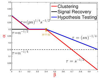
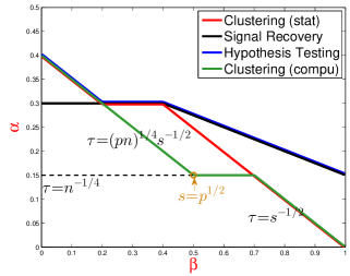
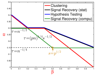
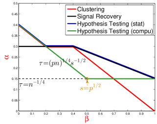
Figure 4: Top left: statistical limits for clustering (red), signal recovery (black), and hypothesis testing (blue); $s=p\epsilon_{p}$. Other three panels: CTUB (green) for clustering (top right), signal recovery (bottom left) and hypothesis testing (bottom right), respectively.

We now present the statistical limits and CTUB for all three problems. They are different from the ones we present in the main paper [28]. First, we look at the statistical limits.

$$\eta^{clu}_{\theta}(\beta)=\left\{\begin{array}[]{ll}(1+\theta-2\beta)/4,&\qquad\beta<(1-\theta)/2,\\ \theta/2,&\qquad(1-\theta)/2<\beta<(1-\theta),\\ (1-\beta)/2,&\qquad\beta>(1-\theta).\end{array}\right.$$

$$\eta^{sig}_{\theta}(\beta)=\left\{\begin{array}[]{ll}\theta/2,&\qquad\beta<(1-\theta),\\ (1+\theta-\beta)/4,&\qquad\beta>(1-\theta).\end{array}\right.$$

$$\eta^{hyp}_{\theta}(\beta)=\left\{\begin{array}[]{ll}(1+\theta-2\beta)/4,&\qquad\beta<(1-\theta)/2,\\ \theta/2,&\qquad(1-\theta)/2<\beta<(1-\theta),\\ (1+\theta-\beta)/4,&\qquad\beta>(1-\theta).\end{array}\right.$$

Figure 4 (top left panel) displays the statistical limits for three problems. Comparing it with Figure 2 (top left panel), we find that : (a) the black curve (signal recovery) remains the same, (b) the red curve (clustering) remains the same, except for the segment on the left is replaced by $\tau^{4}=p/(ns^{2})$, (c) for the blue curve (hypothesis testing), the right most segment remains the same, while the other two segments coincide with those of the red curve.

Achievability. The statistical limit of clustering is achieved by the classical PCA (the left segment) and the variant (A.2) of Sparse Aggregation (the right two segments). For signal recovery, the right two segments are achieved by the modified Sparse Aggregation (A.3), and the left segment is achieved by classical PCA. For hypothesis testing, the left segment is achieved by classical PCA and the right two segments are achieved by the modified Sparse Aggregation (A.4).

Next, we present a CTUB for each of the three problems:

$$\tilde{\eta}^{clu}_{\theta}(\beta)=\left\{\begin{array}[]{ll}(1+\theta-2\beta)/4,&\qquad\beta<1/2,\\ \theta/4,&\qquad 1/2<\beta<1-\theta/2,\\ (1-\beta)/2,&\qquad\beta>(1-\theta).\end{array}\right.$$

$$\tilde{\eta}^{sig}_{\theta}(\beta)=\left\{\begin{array}[]{ll}\theta/2,&\qquad\beta<(1-\theta)/2,\\ (1+\theta-2\beta)/4,&\qquad(1-\theta)/2<\beta<1/2,\\ \theta/4,&\qquad\beta>1/2.\end{array}\right.$$

$$\tilde{\eta}^{hyp}_{\theta}(\beta)=\left\{\begin{array}[]{ll}(1+\theta-2\beta)/4,&\qquad\beta<1/2,\\ \theta/4,&\qquad\beta>1/2.\end{array}\right.$$

See Figure 4 (top right and the two bottom panels).

Methods associated with CTUB. The CTUB for clustering is associated with the methods of classical PCA (left segment) and IF-PCA (right two segments). The CTUB for signal recovery is associated with the methods of classical PCA (left segment) and IF-PCA (right segment). The CTUB for hypothesis testing is associated with the methods of classical PCA (left segment) and IF-PCA (right segment).

Remark. We now make a connection to the recent literature on the Gaussian mixture learning (e.g.[7, 14]). In our framework, we calibrate with $(\epsilon,\tau)$. In the latter, we calibrate with $\|\mu\|$ and $\|\mu\|_{0}$. For brevity, we only discuss the problem of hypothesis testing. The statistical limits for hypothesis testing can be (roughly) re-stated as follows:

• $\sqrt{np}\ll s\ll p$: $s\tau^{2}=\sqrt{p/n}$.

• $n\ll s\ll\sqrt{np}$: $\tau=n^{-1/2}$.

• $s\ll n$: $\tau=(sn)^{-1/4}$.

Note that the first item corresponds to the non-sparse cases in the Gaussian mixture learning literature, where $\|\mu\|^{2}=s\tau^{2}=\sqrt{p/n}$; the results match with those in, e.g., [7, 14]. The second one is part of the sparse case in the Gaussian mixture learning literature, where $1\ll\|\mu\|^{2}=p/n\ll\sqrt{p/n}$ and $n\ll\|\mu\|_{0}\ll\sqrt{np}$. The last one is also part of the sparse case, where $\|\mu\|^{2}=\sqrt{s/n}$ and $s\ll n$.

Appendix B Proof of Lemmas in Section 2

In this sectoin, we prove the post-selection random matrix theory results in Section 2, specifically Lemmas 2.1–2.4.

B.1 Preliminary lemmas for Section 2

Lemma B.1 states the well-known Bernstein inequality [41]. Lemma B.2 is a result from classical Random Matrix Theory [45, Page 21]. Lemma B.3 states some properties about columns of the matrix $Z^{(q)}$; it is proved in Section D.1.

Lemma B.1

Let $X_{1},\cdots,X_{N}$ be independent random variables with $E[X_{k}]=0$ and $\mathrm{var}(X_{k})\leq v_{k}$, for $1\leq k\leq N$. Suppose $E(|X_{k}|^{m})\leq v_{k}m!c^{m-2}/2$ for all $m\geq 2$, where $c>0$ is a constant. Then for all $\lambda>0$,

$$P\big{(}\big{|}\sum_{k=1}^{N}X_{k}\big{|}\geq\lambda\sqrt{N}\big{)}\leq\exp\left(-\frac{\lambda^{2}/2}{\sum_{k=1}^{n}v_{k}/N+c\lambda/\sqrt{N}}\right).$$

Lemma B.2

Let $A$ be an $N\times n$ matrix whose entries are independent standard normal random variables. Then for every $x\geq 0$, with probability at least $1-2\exp(-x^{2}/2)$,

$$\sqrt{N}-\sqrt{n}-x\leq s_{\min}(A)\leq s_{\max}(A)\leq\sqrt{N}+\sqrt{n}+x,$$

where $s_{\min}(A)$ and $s_{\max}(A)$ are the respective minimum and maximum singular values of $A$.

Fix $q>0$. With $e_{1}=(1,0,\cdots,0)^{\prime}$ and $z\sim N(0,I_{p})$, we introduce a few notations:

$$\pi_{0}^{(q)}=P(\|z\|^{2}>n+2\sqrt{qn\log(p)}),$$

$$\pi_{1}^{(q)}=P(\|z+\sqrt{n}\tau_{p}^{*}e_{1}\|^{2}>n+2\sqrt{qn\log(p)}),$$

$$a_{p}^{(q)}=E\big{[}(z(1))^{2}\cdot 1\{\|z\|^{2}>n+2\sqrt{qn\log(p)}\}\big{]},$$

$$b_{p}^{(q)}=E\big{[}(z(2))^{2}\cdot 1\{\|z+\sqrt{n}\tau_{p}^{*}e_{1}\|^{2}>n+2\sqrt{qn\log(p)}\}\big{]},$$

$$c_{p}^{(q)}=E\big{[}(z(1))^{2}\cdot 1\{\|z+\sqrt{n}\tau_{p}^{*}e_{1}\|^{2}>n+2\sqrt{qn\log(p)}\}\big{]}.$$

For notation simplicity, we omit all the superscripts. In the following lemma, $m^{(q)}(\ell,\mu)$, $m_{*}^{(q)}(\ell,\mu)$ and the event $D_{p}$ are defined in Section 2.

Lemma B.3

Let $S(\mu)$ denote the support of $\mu$, $\kappa_{m}=E(|z(1)|^{m})$ and $\kappa_{2m}(n)=E(\|z\|^{2m})$, where $z\sim N(0,I_{n})$. Below, all the probabilities are conditioning on $(\ell,\mu)$, and the $o(1)$ terms are uniform for all realizations of $(\ell,\mu)$ in the event $D_{p}$.

• Fix $j\notin S(\mu)$. For any $v\in\mathcal{S}^{n-1}$ and any integer $m\geq 1$

  $$\begin{array}[]{l}E[(v^{\prime}z_{j}^{(q)})^{2}]=a_{p},\\ E(|v^{\prime}z_{j}^{(q)}|^{m})\leq\kappa_{m}\pi_{0}(1+o(1)),\\ E(\|z_{j}^{(q)}\|^{2})=na_{p},\\ E(\|z_{j}^{(q)}\|^{2m})=\kappa_{2m}(n)\pi_{0}(1+o(1)),\\ a_{p}=\pi_{0}(1+L_{p}n^{-1/2}).\end{array}$$

• Fix $j\in S(\mu)$. For any $v\in\mathcal{S}^{n-1}$ and any integer $m\geq 1$

  $$\begin{array}[]{l}E[(v^{\prime}z_{j}^{(q)})^{2}]=b_{p}+(c_{p}-b_{p})\tfrac{(v^{\prime}\ell)^{2}}{\|\ell\|^{2}}\\ E(|v^{\prime}z_{j}^{(q)}|^{m})\leq\kappa_{m}\pi_{1}(1+o(1)),\\ E(\|z_{j}^{(q)}\|^{2})=nb_{p}+(c_{p}-b_{p}),\\ E(\|z_{j}^{(q)}\|^{2m})\leq 2^{m}\kappa_{2m}(n)\pi_{1}(1+o(1)),\\ b_{p}=\pi_{1}(1+L_{p}n^{-1/4}),\;\;c_{p}=\pi_{1}(1+L_{p}n^{-1/4}).\end{array}$$

• $m^{(q)}(\ell,\mu)=(p-|S(\mu)|)\pi_{0}+|S(\mu)|\pi_{1}$,
  $m_{*}^{(q)}(\ell,\mu)=(p-|S(\mu)|)a_{p}+|S(\mu)|[b_{p}+n^{-1}(c_{p}-b_{p})]$.

Remark. Lemma B.3 allows us to characterize the quantities $m^{(q)}$ and $m^{(q)}_{*}$. First, by (a)-(b), $a_{p}\sim\pi_{0}$ and $b_{p}\sim c_{p}\sim\pi_{1}$. Combining them with (c) gives that $m_{*}^{(q)}\sim m^{(q)}$. Second, we look at $m^{(q)}$. By Lemma D.1 and Mills’ ratio [41], $\pi_{0}\sim\bar{\Phi}(\sqrt{2q\log(p)})=L_{p}p^{-q}$. Similarly, $\pi_{1}\sim L_{p}p^{-[(\sqrt{r}-\sqrt{q})_{+}]^{2}}$. Plugging them into (c) gives

$$m^{(q)}\sim L_{p}p^{1-q}+p\epsilon_{p}\cdot L_{p}p^{-[(\sqrt{r}-\sqrt{q})_{+}]^{2}}.$$

This is the equation (2.1) in the main text of [30].

B.2 Proof of Lemma 2.1

Fix $q>0$ and write $H_{0}=Z^{(q)}(Z^{(q)})^{\prime}$ and $\hat{S}=\hat{S}^{(if)}_{q}$ for short. Fix a realization $(\ell,\mu)$. With probability at least $1-O(p^{-3})$,

$$||\hat{S}|-m^{(q)}|\leq\sqrt{6m^{(q)}\log(p)}.$$ (B.5)

First, we consider $q>\tilde{q}(\beta,\theta,r)$, so that $m^{(q)}\leq np^{-\delta}$ for some $\delta>0$. Let $k=\lceil m^{(q)}+\sqrt{6m^{(q)}\log(p)}\rceil$. Under (B.5),

$$\lambda_{\max}(H_{0})\leq\max_{T\subset\{1,\cdots,p\},|T|\leq k}\lambda_{\max}((ZZ^{\prime})^{T,T}),$$

$$\lambda_{\min}^{+}(H_{0})\geq\min_{T\subset\{1,\cdots,p\},|T|\leq k}\lambda_{\min}^{+}((ZZ^{\prime})^{T,T}),$$

where for a matrix $A$, $\lambda_{\min}^{+}(A)$ denotes the minimum non-zero eigenvalue and $A^{T,T}$ is the submatrix restricted to rows and columns in $T$. For each fixed $T$, we can write $(Z^{\prime}Z)^{T,T}=Z_{T}(Z_{T})^{\prime}$, where $Z_{T}=(z_{j},j\in T)$ is an $n\times|T|$ matrix with iid entries of $N(0,1)$. Using Lemma B.2, for each $T$, with probability at least $1-O(p^{-(k+3)})$, all non-zero eigenvalues of $(ZZ^{\prime})^{T,T}$ fall into

$$\Big{[}\big{(}\sqrt{n}+\sqrt{|T|}+\sqrt{6k\log(p)}\big{)}^{2},\;\big{(}\sqrt{n}-\sqrt{|T|}-\sqrt{6k\log(p)}\big{)}^{2}\Big{]}=n\pm C\sqrt{nk\log(p)}.$$

Note that the number of subsets $T$ such that $|T|\leq k$ is no more than $p^{k}$. Combining the above results, we find that with probability at least $1-O(p^{-3})$, all non-zero eigenvalues of $H_{0}$ fall into

$$n\pm C\sqrt{nm^{(q)}\log(p)}.$$ (B.6)

The claim then follows.

Next, we consider $q<\tilde{q}(\beta,\theta,r)$, so that $m^{(q)}\geq np^{\delta}$ for some $\delta>0$. Write for short

$$\omega_{p}=\sqrt{nm^{(q)}}+o(1)|S(\mu)|\pi_{1},$$

where $\pi_{1}$ is as in Lemma B.3 and $m_{1}^{(q)}=|S(\mu)|\pi_{1}$ by definition. It suffices to show that with probability at least $1-O(p^{-3})$,

$$\|H_{0}-m^{(q)}_{*}I_{n}\|\leq C\omega_{p}.$$ (B.7)

We now show (B.7). Fix $\alpha>0$. A subset $\mathcal{M}_{\alpha}$ of the unit sphere $\mathcal{S}^{n-1}$ is called an $\alpha$-net if for any $v\in\mathcal{S}^{n-1}$, there exits $u\in\mathcal{M}_{\alpha}$ such that $\|u-v\|\leq\alpha$. The following lemma states some well-known results and its proof can be found in [45, Page 8].

Lemma B.4

Fix $\alpha\in(0,1/2)$. For any $\mathcal{M}_{\alpha}$, an $\alpha$-net of $\mathcal{S}^{n-1}$, and any symmetric matrix $A\in R^{n,n}$, $\|A\|\leq(1-2\alpha)^{-1}\sup_{u\in\mathcal{M}_{\alpha}}\{|u^{\prime}Au|\}$. Moreover, there exists an $\alpha$-net $\mathcal{M}^{*}_{\alpha}$ of $\mathcal{S}^{n-1}$ such that $|\mathcal{M}^{*}_{\alpha}|\leq(1+2/\alpha)^{n}$.

By Lemma B.4 with $\alpha=1/4$ , there exists a subset $\mathcal{M}^{*}$, such that $|\mathcal{M}^{*}|\leq 9^{n}$ and $\sup_{v\in\mathcal{M}^{*}}v^{\prime}Av\geq\|A\|/2$ for any $n\times n$ matrix $A$. Therefore, to show the claim, it suffices to show that for each fixed $v\in\mathcal{M}^{*}$, with probability $\geq 1-O(9^{-n}p^{-3})$,

$$|v^{\prime}(H_{0}-m^{(q)}_{*}I_{n})v|\leq C\omega_{p}.$$ (B.8)

We now show (B.8). Fix $v$ and define

$$W_{j}=(v^{\prime}z_{j}^{(q)})^{2}-a_{p},\;\;\mbox{for $j\notin S(\mu)$};\qquad W_{j}=(v^{\prime}z_{j}^{(q)})^{2}-b_{p},\;\;\mbox{for $j\in S(\mu)$},$$

where $a_{p}$ and $b_{p}$ are defined in Section B.1. By (c) of Lemma B.3, $m_{*}^{(q)}=(p-|S(\mu)|)a_{p}+|S(\mu)|b_{p}+n^{-1}(c_{p}-b_{p})|S(\mu)|$. Since $|c_{p}-b_{p}|=o(\pi_{1})$, we can rewrite

$$v^{\prime}(H_{0}-m^{(q)}_{*}I_{n})v=\sum_{j=1}^{p}W_{j}+o(n^{-1}|S(\mu)|\pi_{1}).$$ (B.9)

Here $W_{j}$’s are independent of each other. Applying Lemma B.3, we get the following results. For $j\notin S(\mu)$, $E(W_{j})=0$, $\mathrm{var}(W_{j})\leq 3\pi_{0}(1+o(1))$ and $E(|W_{j}|^{m})\leq\kappa_{2m}\pi_{0}(1+o(1))$. For $j\in S(\mu)$, $|E(W_{j})|\leq|b_{p}-c_{p}|=\pi_{1}\cdot o(1)$, $\mathrm{var}(W_{j})\leq 3\pi_{1}(1+o(1))$ and $E(|W_{j}|^{m})\leq\kappa_{2m}\pi_{1}(1+o(1))$. So we have

$$|\sum_{j=1}^{p}E(W_{j})|=o(1)|S(\mu)|\pi_{1},\qquad\sum_{j=1}^{p}\mathrm{var}(W_{j})\lesssim 3m^{(q)}.$$

We apply Lemma B.1 with $\lambda=\sqrt{9p^{-1}m^{(q)}(n\log(9)+2\log(p)+\log(2))}$. To check the moment conditions, we note that $\kappa_{2m}=E_{Y\sim N(0,1)}(|Y|^{2m})\leq 2^{m}m!$ for all $m\geq 1$. Furthermore, since $m^{(q)}/n\rightarrow\infty$, we have $\sum_{j}\mathrm{var}(W_{j})/p\sim 3m^{(q)}/p\gg\lambda/\sqrt{p}$. It follows that with probability $\geq 1-O(9^{-n}p^{-3})$,

$$|\sum_{j=1}^{p}W_{j}|\lesssim 3\sqrt{\log(9)}\sqrt{nm^{(q)}}+o(1)|S(\mu)|\pi_{1}.$$

This gives (B.8), and the proof is now complete.        $\Box$

B.3 Proof of Lemma 2.2

We have shown the first claim in (B.7), noting that $\omega_{p}\sim\sqrt{nm^{(q)}}$ when $r<\rho^{*}_{\theta}(\beta)$ (see also (B.15)).

We now show the second claim. Write for short $H_{0}=Z^{(q)}(Z^{q})^{\prime}$. The key is the following lemma, which is proved in Section D.

Lemma B.5

Under conditions of Lemma 2.2, as $p\to\infty$, conditioning on any realization of $(\ell,\mu)$ on the event $D_{p}$, with probability at least $1-O(n^{-2})$,

$$|n^{-1}\mathrm{tr}(H_{0})-m_{*}^{(q)}|\leq C\sqrt{m^{(q)}\log(p)},$$

$$\|H_{0}\|^{2}_{F}\geq n^{-1}[\mathrm{tr}(H_{0})]^{2}+Cn^{2}m^{(q)}.$$

Let $k$ be the largest integer that is no larger than $m^{(q)}/2$. Since $k\gg n$, for each fixed $k\times k$ submatrix of $ZZ^{\prime}$, its rank is $n$ with probability $1$. Using (B.5), the rank of $H_{0}$ is $n$ with probability at least $1-O(p^{-3})$. Let $\lambda_{1}\geq\lambda_{2}\geq\cdots\geq\lambda_{n}>0$ be the eigenvalues of $H_{0}$ and write $\bar{\lambda}=n^{-1}\sum_{i=1}^{n}\lambda_{i}$. For $\delta_{p}\equiv\sqrt{nm^{(q)}}$, (B.7) and Lemma B.5 imply

$$|\lambda_{1}-\lambda_{n}|\leq A_{1}\delta_{p},\qquad\bar{\lambda}=m_{*}^{(q)}+o(\delta_{p}),\qquad\sum_{i=1}^{n}\lambda_{i}^{2}\geq n\bar{\lambda}^{2}+A_{2}n\delta_{p}^{2},$$ (B.10)

for some constants $A_{1},A_{2}>0$. On one hand,

$$\sum_{i=1}^{n}(\lambda_{i}-\bar{\lambda})^{2}\geq A_{2}n\delta_{p}^{2}.$$

On the other hand, $\lambda_{i}-\bar{\lambda}\leq\lambda_{1}-\bar{\lambda}$ for $i$ satisfying $\lambda_{i}\geq\bar{\lambda}$; moreover, $\bar{\lambda}-\lambda_{i}\leq A_{1}\delta_{p}$ for $i$ such that $\lambda_{i}<\bar{\lambda}$. It follows that

$$\sum_{i=1}^{n}(\lambda_{i}-\bar{\lambda})^{2} \leq(\lambda_{1}-\bar{\lambda})\sum_{i:\lambda_{i}\geq\bar{\lambda}}(\lambda_{i}-\bar{\lambda})+A_{1}\delta_{p}\sum_{i:\lambda_{i}<\bar{\lambda}}(\bar{\lambda}-\lambda_{i})$$

$$=[(\lambda_{1}-\bar{\lambda})+A_{1}\delta_{p}]\sum_{i:\lambda_{i}\geq\bar{\lambda}}(\lambda_{i}-\bar{\lambda})$$

$$\leq n[(\lambda_{1}-\bar{\lambda})+A_{1}\delta_{p}](\lambda_{1}-\bar{\lambda}).$$

Now, if we write $x=\lambda_{1}-\bar{\lambda}$, then $x(x+A_{1}\delta_{p})\geq A_{2}\delta_{p}^{2}$. It follows that

$$\lambda_{1}-\bar{\lambda}\geq\frac{\sqrt{A_{1}^{2}+4A_{2}}-A_{1}}{2}\delta_{p}.$$ (B.11)

Combining it with the second equation in (B.10), we obtain that $\lambda_{1}\geq m^{(q)}_{*}+C\sqrt{nm^{(q)}}$.        $\Box$

B.4 Proof of Lemma 2.3

Write for short $A=\ell(Z^{(q)}\mu^{(q)})^{\prime}+(Z^{(q)}\mu^{(q)})\ell^{\prime}$. Since

$$\|A\|\leq 2\|\ell\|\|Z^{(q)}\mu^{(q)}\|\leq 2n\|Z^{(q)}\mu^{(q)}\|_{\infty},$$

it suffices to show that with probability $1-O(p^{-3})$,

$$\|Z^{(q)}\mu^{(q)}\|_{\infty}\leq C\tau_{p}^{*}\sqrt{m_{1}^{(q)}}.$$ (B.12)

Note that

$$\|Z^{(q)}\mu^{(q)}\|_{\infty}=\max_{1\leq i\leq n}|\sum_{j\in S(\mu)}\mu(j)z_{j}^{(q)}(i)|=\tau_{p}^{*}\max_{1\leq i\leq n}|\sum_{j\in S(\mu)}z_{j}^{(q)}(i)|.$$ (B.13)

Fix $i$ and write $V_{j}=z_{j}^{(q)}(i)$ for short. Then $V_{j}$’s are independent and $E(V_{j})=0$ by symmetry. We apply Lemma B.3 with $v=e_{1}$ and find that $\mathrm{var}(V_{j})\leq b_{p}+2|c_{p}-b_{p}|=\pi_{1}(1+o(1))$. By Lemma B.1 (the moment conditions can be verified using Lemma B.3), $|\sum_{j\in S(\mu)}V_{j}|\leq 2\sqrt{|S(\mu)|\pi_{1}}$ with probability $1-O(p^{-4})$. It follows that with probability $1-O(p^{-3})$,

$$\max_{1\leq i\leq n}|\sum_{j\in S(\mu)}z_{j}^{(q)}(i)|\leq C\sqrt{|S(\mu)|\pi_{1}}=C\sqrt{m_{1}^{(q)}}.$$ (B.14)

Combining (B.13)-(B.14) gives (B.12).        $\Box$

B.5 Proof of Lemma 2.4

Introduce

$$\Delta^{{\dagger}}(q,\beta,r,\theta)$$

$$= \left\{\begin{array}[]{ll}\beta-\frac{1}{2}\min\{q,\beta-\frac{\theta}{2}\},&q\leq r,\\ \beta+(\sqrt{q}-\sqrt{r})^{2}-\frac{1}{2}\min\{q,\beta-\frac{\theta}{2}+(\sqrt{q}-\sqrt{r})^{2}\},&q>r.\end{array}\right.$$

By elementary algebra,

$$r<\rho^{*}_{\theta}(\beta)\qquad\Longleftrightarrow\qquad\min_{q>0}\Delta^{{\dagger}}(q,\beta,r,\theta)>1/2,$$

Moreover, using Mills’ ratio,

$$\min\left\{\frac{n(\tau_{p}^{*})^{2}|S(\mu)|\pi_{1}}{\sqrt{nm^{(q)}}},\;\;\tau_{p}^{*}\sqrt{|S(\mu)|\pi_{1}}\right\}=L_{p}p^{1/2-\Delta^{{\dagger}}(q,\beta,r,\theta)}.$$

It follows that for some $\delta>0$,

$$r<\rho^{*}_{\theta}(\beta)\qquad\Longleftrightarrow\qquad|S(\mu)|\pi_{1}\leq p^{-\delta}\max\{\sqrt{m^{(q)}},\sqrt{n}\}.$$ (B.15)

Consider the first claim. The proof is similar to that of (B.8), except that we take $\lambda=C\sqrt{p^{-1}m^{(q)}\log(p)}$ when applying Lemma B.1. It follows that for any $v\in\mathcal{S}^{n-1}$, with probability at least $1-O(p^{-3})$,

$$|v^{\prime}(H_{0}-m^{(q)}_{*}I_{n})v|\leq C\sqrt{m^{(q)}\log(p)}+o(|S(\mu)|\pi_{1}).$$

By (B.15), the second term above is negligible and the claim follows.

Consider the second claim. $H-H_{0}=\|\mu^{(q)}\|^{2}\ell\ell^{\prime}+A$, where with probability at least $1-O(p^{-3})$, $\|A\|\leq Cn\tau_{p}^{*}\sqrt{m_{1}^{(q)}}$ by Lemma 2.3. Furthermore, by elementary statistics, $\|\mu^{(q)}\|^{2}\leq Cm_{1}^{(q)}(\tau_{p}^{*})^{2}$. Note that $m_{1}^{(q)}=|S(\mu)|\pi_{1}$ due to the spherical symmetry of $N(0,I_{n})$. Together, we see that

$$\|H-H_{0}\|\leq L_{p}(\sqrt{n}|S(\mu)|\pi_{1}+n^{3/4}\sqrt{|S(\mu)|\pi_{1}}).$$

If $q>\tilde{q}(\beta,r,\theta)$, then $m^{(q)}=o(n)$ and (B.15) implies $\|H-H_{0}\|\leq p^{-\delta}n$. If $q<\tilde{q}(\beta,r,\theta)$, then $n=o(m^{(q)})$ and (B.15) implies $\|H-H_{0}\|\leq p^{-\delta}\sqrt{nm^{(q)}}$.        $\Box$

Appendix C Proof of Lemmas in Section 3

In this section, we prove Lemmas 3.1–3.3.

C.1 Proof of Lemma 3.1

We first show the claim for $B=I_{p}$ and then generalize it to any $B$ satisfying $\max\{\|B\|,\|B^{-1}\|\}\leq L_{p}$.

Fix $B=I_{p}$. We use $\delta>0$ to denote a generic constant which only depends on $(\alpha,\beta,\theta)$ but may change from occurrence to occurrence. In our model, $X=\ell\mu^{\prime}+Z$. Let $H_{0}=ZZ^{\prime}-pI_{n}$. It is seen

$$XX^{\prime}-pI_{n}=[\|\mu\|^{2}\ell\ell^{\prime}+\ell\mu^{\prime}Z^{\prime}+Z\mu\ell^{\prime}]+ZZ^{\prime}-pI_{n}=[\|\mu\|^{2}\ell\ell^{\prime}+\ell\mu^{\prime}Z^{\prime}+Z\mu\ell^{\prime}]+H_{0}.$$ (C.16)

Since $\xi$ is a left singular vector of $X$, $\lambda\xi=[\|\mu\|^{2}(\xi,\ell)+(\xi,Z\mu)]\ell+(\xi,\ell)Z\mu+H_{0}\xi$. Rearranging it, we have

$$\sqrt{n}\xi=(I_{n}-(1/\lambda)H_{0})^{-1}[b_{1}\ell+b_{2}Z(\mu/\|\mu\|)],$$ (C.17)

where $b_{1}=b_{1}(\ell,Z,\mu)=(1/\lambda)\cdot[\sqrt{n}\|\mu\|^{2}(\xi,\ell)+\sqrt{n}(\xi,Z\mu)]$ and $b_{2}=b_{2}(\ell,Z,\mu)=(1/\lambda)\sqrt{n}\|\mu\|(\xi,\ell)$. Therefore, $\min\{\|\sqrt{n}\xi-\ell\|_{\infty},\|\sqrt{n}\xi+\ell\|_{\infty}\}$ is no greater than

$$\min\{|b_{1}-1|,|b_{1}+1|\}+|b_{1}|\|\ell-(I_{n}-(1/\lambda)H_{0})^{-1}\ell\|_{\infty}+|b_{2}|\|(I_{n}-(1/\lambda)H_{0})^{-1}Z(\mu/\|\mu\|)\|_{\infty}.$$ (C.18)

To show the claim, it is sufficient to show that with probability at least $1-o(p^{-3})$,

$$\min\{|b_{1}-1|,|b_{1}+1|\}\leq p^{-\delta},\qquad|b_{2}|\leq p^{-\delta},$$ (C.19)

and

$$\|\ell-(I_{n}-(1/\lambda)H_{0})^{-1}\ell\|_{\infty}\leq p^{-\delta},\qquad\|(I_{n}-\frac{1}{\lambda}H_{0})^{-1}Z(\mu/\|\mu\|)\|_{\infty}\leq C\sqrt{\log(p)}.$$ (C.20)

We now show (C.19). Consider the first item. Since $Z$ and $\mu$ are independent, we have that with probability at least $1-o(p^{-3})$, $|(\xi,Z\mu)|\leq\|\mu\|\cdot\|Z(\mu/\|\mu\|)\|\leq 2\|\mu\|\sqrt{n}$. Combining this with the triangle inequality,

$$\min\{b_{1}-1,b_{1}+1\}$$

$$\leq (n\|\mu\|^{2}/\lambda)|\mathrm{cos}(\ell,\xi)-1|+|1-(n\|\mu\|^{2}/\lambda)|+(\sqrt{n}/\lambda)|(\xi,Z\mu)|$$

$$\leq (n\|\mu\|^{2}/\lambda)|\mathrm{cos}(\ell,\xi)-1|+|1-(n\|\mu\|^{2}/\lambda)|+2n\|\mu\|/\lambda.$$ (C.21)

At the same time, we rewrite (C.16) as

$$XX^{\prime}-pI_{n}=A+H_{0},\;\mbox{where $A=\|\mu\|^{2}\ell\ell^{\prime}+\ell\mu^{\prime}Z^{\prime}+Z\mu\ell^{\prime}$ for short}.$$ (C.22)

Note that $A$ is a symmetric matrix of rank $2$. For short, write $\nu=\|\mu\|^{-2}\mu$ and $a=a(\ell,\mu,Z)=(1+4n^{-1}[\ell^{\prime}Z\nu+\|Z\nu\|^{2}])^{1/2}$. Let $\lambda_{\pm}$ be the two nonzero eigenvalues of $A$, and let $\eta_{\pm}$ be the corresponding eigenvectors. By elementary algebra,

$$\lambda_{\pm}(A)=n\|\mu\|^{2}[(1/2)(1\pm a)+n^{-1}\ell^{\prime}Z\nu],\qquad\eta_{\pm}\propto(1/2)(1\pm a)\ell+Z\nu.$$ (C.23)

By elementary statistics, it is seen that with probability at least $1-o(p^{-3})$ that $n^{-1}[|\ell^{\prime}Z\nu|+\|Z\nu\|^{2}]$ does not exceed

$$C\sqrt{\log(p)}n^{-1}[(\sqrt{n}\|\mu\|^{-1})+n\|\mu\|^{-2}]=C\sqrt{\log(p)}[(\sqrt{n}\|\mu\|)^{-1}+\|\mu\|^{-2}].$$ (C.24)

Note that for $(\alpha,\beta,\theta)$ in our range of interest, $p\epsilon_{p}\tau_{p}^{2}\geq\sqrt{p/n}=p^{(1-\theta)/2}$. By the way $\mu$ is generated, $\|\mu\|^{2}\sim p\epsilon_{p}\tau_{p}^{2}$. Therefore, with probability at least $1-o(p^{-3})$,

$$\|\mu\|^{2}\sim p\epsilon_{p}\tau_{p}^{2}\geq p^{\delta}\sqrt{p/n},\qquad n\|\mu\|^{2}\sim np\epsilon_{p}\tau_{p}^{2}\geq p^{\delta}\sqrt{pn}.$$ (C.25)

Inserting (C.25) into (C.24) gives that with probability at least $1-o(p^{-3})$, $|a-1|\leq Cp^{-\delta}$. Combining this with (C.23),

$$|(n\|\mu\|^{2}/\lambda_{+})-1|\leq p^{-\delta},\qquad(\lambda_{-}/\lambda_{+})\leq p^{-\delta},\qquad|\mathrm{cos}(\ell,\eta_{+})-1|\leq p^{-\delta}.$$ (C.26)

At the same time, by a direct use of the elementary Random Matrix Theory [45], $\|H_{0}\|=\|ZZ^{\prime}-pI_{p}\|\leq C\sqrt{pn}$. Combining these with (C.25)-(C.26) gives

$$\|(1/\lambda_{+})H_{0}\|\leq C\sqrt{pn}/(n\|\mu\|^{2})\leq Cp^{-\delta}.$$ (C.27)

This says that in (C.22), the leading eigenvalue of $A$ is larger than that of $H_{0}$ by $p^{\delta}$ times. By matrix perturbation theory, we have that with probability at least $1-o(p^{-3})$,

$$|\lambda_{+}/\lambda-1|\leq p^{-\delta},\qquad|\mathrm{cos}(\eta_{+},\xi)-1|\leq p^{-\delta}.$$ (C.28)

Combining (C.26) and (C.28) gives

$$|(n\|\mu\|^{2}/\lambda)-1|\leq p^{-\delta},\qquad|\mathrm{cos}(\ell,\xi)-1|\leq p^{-\delta}.$$ (C.29)

In particular, combining (C.25), (C.27), and (C.28) gives that with probability at least $1-o(p^{-3})$,

$$\|(1/\lambda)H_{0}\|\leq Cp^{-\delta},\qquad\sqrt{pn}/\lambda\leq p^{-\delta}.$$ (C.30)

Inserting (C.29) into (C.21) gives the first item of (C.19).

Consider the second item of (C.19). Note that $|b_{2}|\leq(n\|\mu\|/\lambda)$, where by (C.29), the right hand side $\leq\|\mu\|^{-1}$. The claim follows directly from (C.25).

We now show (C.20). Since the proofs are similar, we only show the first item. Let $e_{1}$ be the first base vector of $R^{n}$. Note that by symmetry and by using the union bound, it is sufficient to show that with probability at least $1-o(p^{-4})$,

$$\bigl{|}e_{1}^{\prime}(I_{n}-\frac{1}{\lambda}H_{0})^{-1}e_{1}-1\bigr{|}\leq p^{-\delta},\qquad|e_{1}^{\prime}(I_{n}-\frac{1}{\lambda}H_{0})^{-1}(\ell-\ell_{1}e_{1})|\leq C\sqrt{\log(p)}.$$ (C.31)

The first claim follows easily by (C.30) and basic algebra. For the second claim, write $\ell=(\ell_{1},\tilde{\ell})^{\prime}$, and let $\tilde{Z}$ be the $(n-1)\times p$ matrix consisting all but the first row of $Z$, and let $\tilde{H}_{0}=\tilde{Z}\tilde{Z}^{\prime}-pI_{n-1}$. It follows that

$$I_{n}-(1/\lambda)H_{0}=\left(\begin{array}[]{ll}1-(1/\lambda)[\|Z_{1}\|^{2}-p],&-(1/\lambda)Z_{1}^{\prime}\tilde{Z}\\ -(1/\lambda)\tilde{Z}Z_{1},&I_{n-1}-(1/\lambda)\tilde{H}_{0}\end{array}\right),$$

and

$$e_{1}^{\prime}(I_{n}-\frac{1}{\lambda}H_{0})^{-1}(\ell-\ell_{1}e_{1})=(e_{1}^{\prime}[I_{n}-(1/\lambda)H_{0}]^{-1}e_{1})\cdot(1/\lambda)Z_{1}^{\prime}\tilde{Z}^{\prime}[I_{n-1}-(1/\lambda)\tilde{H}_{0}]^{-1}\tilde{\ell}.$$ (C.32)

Now, since rows of $Z$ are independent, $Z_{1}$ and $\tilde{Z}[I_{n-1}-(1/\lambda)\tilde{H}_{0}]^{-1}\tilde{\ell}$ are two vectors that almost independent of each other; the only issue is that $Z_{1}$ is correlated with $\lambda$. To overcome the difficulty, we write

$$\frac{Z_{1}^{\prime}\tilde{Z}^{\prime}[I_{n-1}-(1/\lambda)\tilde{H}_{0}]^{-1}\tilde{\ell}}{\lambda}=\sum_{k=0}^{\infty}\frac{Z_{1}^{\prime}\tilde{Z}\tilde{H}_{0}^{k}\tilde{\ell}}{\lambda^{k+1}}=\sum_{k=0}^{\infty}\frac{\|\tilde{Z}\tilde{H}_{0}^{k}\tilde{\ell}\|}{\lambda^{k+1}}\cdot\frac{Z_{1}^{\prime}\tilde{Z}\tilde{H}_{0}^{k}\tilde{\ell}}{\|\tilde{Z}\tilde{H}_{0}^{k}\tilde{\ell}\|}.$$ (C.33)

Now, for each $k$, $Z_{1}$ and $\tilde{Z}\tilde{H}_{0}^{k}\tilde{\ell}$ are independent, and so

$$Z_{1}^{\prime}(\tilde{Z}^{\prime}\tilde{H}_{0}^{k}\tilde{\ell}/\|\tilde{Z}^{\prime}\tilde{H}_{0}^{k}\tilde{\ell}\|)\sim N(0,1).$$

For $k$-th term, with probability $1-o(p^{-4(k+1)})$, there is $|Z_{1}^{\prime}(\tilde{Z}^{\prime}\tilde{H}_{0}^{k}\tilde{\ell}/\|\tilde{Z}^{\prime}\tilde{H}_{0}^{k}\tilde{\ell}\|)|\leq\sqrt{8(k+1)\log(p)}$. Additionally, by basics in RMT [45], with probability at least $1-o(p^{-4})$, $\|\tilde{Z}\tilde{H}_{0}^{k}\|\leq\sqrt{p}(C\sqrt{np})^{k}$ for all $k$.

$$(1/\lambda)^{k+1}\|\tilde{Z}\tilde{H}_{0}^{k}\tilde{\ell}\|\leq\sqrt{(n-1)}(1/\lambda)^{k}\|\tilde{Z}\tilde{H}_{0}^{k}\|\leq(C\sqrt{np}/\lambda)^{k+1}.$$

Combining these with (C.33) and the second term of (C.30), it is seen that with probability at least $1-o(p^{-4})$,

$$|(1/\lambda)Z_{1}^{\prime}\tilde{Z}^{\prime}[I_{n-1}-(1/\lambda)\tilde{H}_{0}]^{-1}\tilde{\ell}|\leq p^{-\delta}.$$

Inserting this into (C.32) and using the first item of (C.31), the second item of (C.31) follows.

For a general $B$, the proof is similar by noting that $\|ZB\|\leq L_{p}\|Z\|$ and the following lemma, which is proved below.

Lemma C.1

As $n,p\rightarrow\infty$ and $p/n\rightarrow\infty$, for an $n\times p$ random matrix $Z$ where $Z(i,j)\overset{iid}{\sim}N(0,1)$ and any non-random matrix $B\in R^{p,p}$ such that $\max\{\|B\|,\|B^{-1}\|\}\leq L_{p}$, with probability $1-O(p^{3})$, $\|ZBB^{\prime}Z^{\prime}-\mathrm{tr}(BB^{\prime})I_{n}\|\leq C\sqrt{np}$.

C.2 Proof of Lemma 3.2

Letting $\Phi$ be the CDF of $N(0,1)$, denote the mean and variance of $|z_{i}+h|$ by $u(h)$ and $\sigma^{2}(h)$, respectively. It is seen that

$$u(h)=\sqrt{2/\pi}e^{-h^{2}/2}+h[1-2\Phi(-h)],\qquad\sigma^{2}(h)=1+h^{2}-\mu^{2}(h).$$ (C.34)

By Jensen’s inequality, $E|z_{i}+h|\geq|E(z_{i}+h)|=h$. It follows that

$$u(h)\geq h,\qquad\sigma^{2}(h)\leq 1,$$ (C.35)

At the same time, we claim that as $n\rightarrow\infty$, for any $0\leq x\leq\sqrt{n}/\log(n)$,

$$P\bigl{(}\bigl{|}\sum_{i=1}^{n}\bigl{(}|z_{i}+h|-u(h)\bigr{)}\bigr{|}\geq\sqrt{n}x\bigr{)}\leq 2\mathrm{exp}\bigl{(}-(1+o(1))\frac{x^{2}}{2\sigma^{2}(h)}\bigr{)},$$ (C.36)

where $o(1)\rightarrow 0$ as $n\rightarrow\infty$, uniformly for all $h>0$ and $0<x\leq\sqrt{n}/\log(n)$. Combining (C.35) and (C.36) gives Lemma 3.2.

We now show (C.36). Write for short $Y_{i}=|z_{i}+h|$. It is sufficient to show that

$$P\bigl{(}\sum_{i=1}^{n}Y_{i}\geq nu(h)+\sqrt{n}x\bigr{)}\leq\mathrm{exp}\bigl{(}-(1+o(1))\frac{x^{2}}{2\sigma^{2}(h)}\bigr{)},$$ (C.37)

and

$$P\bigl{(}\sum_{i=1}^{n}Y_{i}\leq nu(h)-\sqrt{n}x\bigr{)}\leq\mathrm{exp}\bigl{(}-(1+o(1))\frac{x^{2}}{2\sigma^{2}(h)}\bigr{)}.$$ (C.38)

Since the proofs are similar, we only show (C.37). By elementary calculations, the moment generating function of $Y_{i}$ is

$$M_{Y}(s)=E[e^{sY}]=e^{s^{2}/2}[e^{hs}\Phi(s+h)+e^{-hs}\Phi(s-h)],$$ (C.39)

By Cramer-Chernoff Theorem ([10]), for any $s>0$ and any $y$,

$$P(\sum_{i=1}^{n}Y_{i}\geq ny)\leq e^{-n(ys-\log M_{Y}(s))}.$$ (C.40)

We now show this (C.37) for the cases of $h<2\log(\sqrt{n}/x)$ and $h\geq 2\log(\sqrt{n}/x)$ separately.

Consider the case where $h<2\log(\sqrt{n}/x)$. We wish to use (C.40) with

$$s=\frac{1}{\sigma^{2}(h)}\frac{x}{\sqrt{n}},\qquad y=u(h)+x/\sqrt{n}.$$

By our assumptions of $h<2\log(\sqrt{n}/x)$ and $0<x\leq\sqrt{n}/\log(n)$,

$$s=O(x/\sqrt{n})=o(1),\qquad hs\leq 2\log(\sqrt{n}/x)(x/\sqrt{n})=o(1).$$

Now, on one hand, since $y\log^{3}(1/y)\rightarrow 0$ as $y\rightarrow 0+$, $h^{3}s=o(1)$ and $h^{3}s^{3}=o(s^{2})$. Combining this with elementary Taylor expansion,

$$e^{\pm hs}=1\pm hs+\frac{(hs)^{2}}{2}+o(s^{2}).$$ (C.41)

On the other hand, applying Taylor expansion to $\Phi(s\pm h)$ and noting that $\phi$ is a symmetric function,

$$\Phi(s\pm h)=\Phi(\pm h)+\phi(h)s-h\phi(h)s^{2}+o(s^{2}).$$ (C.42)

where we have used that the third derivative of $\Phi$ is a bounded function. Combining (C.41)-(C.42) and re-arranging,

$$e^{hs}\Phi(s+h)+e^{-hs}\Phi(s-h)$$ (C.43)

$$= 1+2s\phi(h)+hs[\Phi(h)-\Phi(-h)]+h^{2}s^{2}/2+o(s^{2})$$

$$= 1+u(h)s+h^{2}s^{2}/2+o(s^{2}),$$ (C.44)

where in the first step, we have used $\Phi(h)+\Phi(-h)=1$, and in the second step, we have used the expression of $u(h)$ given in (C.34).

We now analyze $\log[e^{hs}\Phi(s+h)+e^{-hs}\Phi(s-h)]$. Write for short $w=e^{hs}\Phi(s+h)+e^{-hs}\Phi(s-h)-1$. By (C.44) and $|u(h)|\leq h+1$ from (C.34), $|w|\leq C\max\{(h+1)s,h^{2}s^{2}\}$, and so

$$|\log(1+w)-w+w^{2}/2|\leq C|w|^{3}\leq C\max\{(h+1)^{3}s^{3},h^{6}s^{6}\},$$

where by similar argument as above, $\max\{(h+1)^{3}s^{3},h^{6}s^{6}\}=o(s^{2})$. Combining this with (C.44),

$$\log[e^{hs}\Phi(s+h)+e^{-hs}\Phi(s-h)]$$

$$= \log(1+w)$$

$$= w-w^{2}/2+o(s^{2})$$

$$= u(h)s+h^{2}s^{2}/2-[u(h)s+h^{2}s^{2}/2]^{2}/2+o(s^{2})$$

$$= u(h)s+(h^{2}-u(h)^{2})s^{2}/2-[u(h)h^{2}s^{3}+h^{4}s^{4}/4]/2+o(s^{2}),$$

where we note $|u(h)h^{2}s^{3}+h^{4}s^{4}/4|\leq C(h+1)h^{2}s^{3}+h^{4}s^{4}/4=o(s^{2})$. As a result,

$$\log[e^{hs}\Phi(s+h)+e^{-hs}\Phi(s-h)]=u(h)s+(h^{2}-u(h)^{2})s^{2}/2+o(s^{2}).$$

Combining this with (C.39) and the expression of $\sigma(h)$ given in (C.34) and rearranging it,

$$ys-\log[M_{Y}(s)]=(y-u(h))s-(1+h^{2}-u(h)^{2})\frac{s^{2}}{2}+o(s^{2})=(y-u(h))s-\sigma^{2}(h)\frac{s^{2}}{2}+o(s^{2}).$$

Now, invoking $s=\frac{1}{\sigma^{2}(h)}x/\sqrt{n}$ and $y=u(h)+x/\sqrt{n}$ gives

$$ys-\log[M_{Y}(s)]=\frac{1}{2\sigma^{2}(h)}(x/\sqrt{n})^{2}(1+o(1)).$$

Combining this with (C.40) gives the claim.

We now consider the case of $h\geq 2\log(\sqrt{n}/x)$. We wish to use (C.40) again, with the same $y$ but a different $s$: $s=x/\sqrt{n}$. In the current case, since $x\leq\sqrt{n}/\log(n)$,

$$h\rightarrow\infty,\qquad s\rightarrow 0.$$

By the assumptions of $h\geq 2\log(\sqrt{n}/x)$ and $s=x/\sqrt{n}$, and

$$\phi(h/2)\leq C\mathrm{exp}(-(\log(\sqrt{n}/x))^{2}/2)=o(s^{2}),$$

it follows that $\max\{\Phi(-s-h),\Phi(s-h)\}\leq\Phi(-h/2)=o(1)\phi(h/2)$, where the right hand side is $o(s^{2})$. As a result,

$$e^{hs}\Phi(s+h)+e^{-hs}\Phi(s-h)=e^{hs}[1-\Phi(-s-h)+e^{-2hs}\Phi(s-h)]=e^{hs}[1+o(s^{2})],$$ (C.45)

and so

$$\log[e^{hs}\Phi(s+h)+e^{-hs}\Phi(s-h)]=hs+o(s^{2}).$$

Combining this with (C.39) and (C.47) and invoking $s=x/\sqrt{n}$ and $y=u(h)+x/\sqrt{n}$,

$$ys-\log M_{Y}(s) =(u(h)+x/\sqrt{n}-h)s-s^{2}/2+o(s^{2})$$

$$=s^{2}/2+o(s^{2})$$

$$=s^{2}/(2\sigma^{2}(h))+o(s^{2}),$$ (C.46)

where in the last two steps, we have used

$$h-u(h)=2h\Phi(-h)-2\phi(h)=o(s),\qquad\sigma^{2}(h)=1+h^{2}-u(h)^{2}=1+o(s).$$ (C.47)

Inserting (C.46) into (C.40) gives the claim.        $\Box$

C.3 Proof of Lemma 3.3

Denote by $\Phi$ the CDF of $N(0,1)$. By direct calculations,

$$u(h)=\sqrt{2/\pi}e^{-h^{2}/2}+h[1-2\Phi(-h)].$$

This implies $u(h)\rightarrow\sqrt{2/\pi}$ when $h\rightarrow 0$ and $u(h)/h\rightarrow 1$ when $h\rightarrow\infty$. Furthermore,

$$u^{\prime}(h)=-2h\phi(h)+[1-2\Phi(-h)]+2h\phi(-h)=1-2\Phi(-h),$$

$$u^{\prime\prime}(h)=2\phi(-h)>0.$$

So $u(h)$ is strictly convex and monotony increasing for $h\in(0,\infty)$.

Let $h_{0}$ be the unique solution of $u^{\prime}(h)=0.9$. Fix $(h_{1},h_{2})$ such that $h_{2}>h_{1}>0$. If $h_{1}>h_{0}$, by convexity,

$$u(h_{2})-u(h_{1})\geq u^{\prime}(h_{1})(h_{2}-h_{1})\geq 0.9(h_{2}-h_{1}).$$

If $h_{2}<h_{0}$, using the Taylor expansion, for some $\tilde{h}\in[h_{1},h_{2}]$,

$$u(h_{2})-u(h_{1})=u^{\prime}(h_{1})(h_{2}-h_{1})+\frac{1}{2}u^{\prime\prime}(\tilde{h})(h_{2}-h_{1})^{2}\geq\frac{1}{2}u^{\prime\prime}(h_{0})(h_{2}-h_{1})^{2}.$$

If $h_{1}<h_{0}<h_{2}$, then we decompose the difference into $u(h_{2})-u(h_{0})+u(h_{0})-u(h_{1})$ and combine with the two cases we just dicussed, then we have that

$$u(h_{2})-u(h_{1})\geq 0.9(h_{2}-h_{0})+C_{1}(h_{0}-h_{1})^{2}.$$

When $h_{2}-h_{0}\geq h_{0}-h_{1}$, then we have $u(h_{2})-u(h_{1})\geq 0.45(h_{2}-h_{0})+0.45(h_{0}-h_{1})=0.45(h_{2}-h_{1})$; otherwise, there is $u(h_{2})-u(h_{1})\geq\frac{C_{1}}{2}[(h_{2}-h_{0})^{2}+(h_{0}-h_{1})^{2}]\geq C(h_{2}-h_{1})^{2}$. Combining the three cases gives the claim.        $\Box$

Appendix D Proof of Secondary Lemmas

In this section, we show the proof of Lemmas B.3, B.5 and C.1.

D.1 Proof of Lemma B.3

The following lemma is useful, which is proved below.

Lemma D.1

For any fixed $q>0$,

$$\pi_{0}^{(q)}=\bar{\Phi}\big{(}\sqrt{2q\log(p)}\big{)}\big{(}1+L_{p}n^{-1/2}\big{)},$$

$$\pi_{1}^{(q)}=\left\{\begin{array}[]{ll}1-L_{p}p^{-(\sqrt{r}-\sqrt{q})^{2}},&r>q,\\ \bar{\Phi}\big{(}(\sqrt{q}-\sqrt{r})\sqrt{2\log(p)}\big{)}\big{(}1+L_{p}n^{-1/4}\big{)},&r\leq q.\end{array}\right.$$

First, we prove (a). Write for short $z_{j}=z$ and $z^{(q)}=z_{j}^{(q)}$. Since the distribution of $z^{(q)}$ is spherically symmetric, $v^{\prime}z^{(q)}$ has the same distribution as $e_{1}^{\prime}z^{(q)}$, for any $v\in\mathcal{S}^{n-1}$. It follows that $E[(v^{\prime}z^{(q)})^{2}]=E[(z^{(q)}(1))^{2}]=a_{p}$. Furthermore, $E(\|z^{(q)}\|^{2})=nE[(z^{(q)}(1))^{2}]=na_{p}$.

Consider $E(|v^{\prime}z^{(q)}|^{m})$. Again, by spherical symmetry,

$$E(|v^{\prime}z^{(q)}|^{m})=E\big{(}|z^{(q)}(1)|^{m}\big{)}=E\big{(}|z(1)|^{m}1\{z^{2}(1)+\|\tilde{z}\|^{2}>n+2\sqrt{qn\log(p)}\}\big{)},$$

where $\tilde{z}=(z(2),\cdots,z(n))^{\prime}$. Note that $\tilde{z}$ is independent of $z(1)$ and $\|\tilde{z}\|^{2}\sim\chi^{2}_{n-1}$. Let $B_{1}$ be the event that $|z(1)|\leq\sqrt{2\delta_{1}\log(p)}$, for some $\delta_{1}$ to determine. From basic properties of the $N(0,1)$ distribution, $P(B_{1}^{c})=L_{p}p^{-\delta_{1}}$ and $E(|z(1)|^{m}I_{B_{1}^{c}})=L_{p}p^{-\delta_{1}}$. It follows that

$$E(|v^{\prime}z^{(q)}|^{m}) \leq E\big{(}|z(1)|^{m}1\{z^{2}(1)+\|\tilde{z}\|^{2}>n+2\sqrt{qn\log(p)},B_{1}\}\big{)}+L_{p}p^{-\delta_{1}}$$

$$\leq E\big{(}|z(1)|^{m}1\{\|\tilde{z}\|^{2}>n+2\sqrt{qn\log(p)}-2\sqrt{\delta_{1}\log(p)}\}\big{)}+L_{p}p^{-\delta_{1}}$$

$$=E(|z(1)|^{m})\cdot P(\|\tilde{z}\|^{2}>n+2\sqrt{qn\log(p)}(1+o(1)))+L_{p}p^{-\delta_{1}}$$

$$=E(|z(1)|^{m})\pi_{0}(1+o(1))+L_{p}p^{-\delta_{1}}.$$

By choosing $\delta_{1}$ appropriately large, we find that the first term dominates.

Consider $E(\|z^{(q)}\|^{2m})$. Denote by $f_{n}$ the density of $\chi^{2}_{n}$, where $f_{n}(y)=\frac{y^{n/2-1}e^{-y}}{2^{n/2}\Gamma(n/2)}$. Note that $y^{m}f_{n}(y)=\frac{2^{m}\Gamma(m+n/2)}{\Gamma(n/2)}f_{n+2m}(y)$. It follows that

$$E(\|z^{(q)}\|^{2m})=\frac{2^{m}\Gamma(m+n/2)}{\Gamma(n/2)}P(\chi^{2}_{n+2m}>n+2\sqrt{qn\log(p)}).$$

First, by letting $q=0$ on both hand sides, we have $\kappa_{2m}(n)=E(\|z\|^{2m})=\frac{2^{m}\Gamma(m+n/2)}{\Gamma(n/2)}$. Second, since $n+2\sqrt{qn\log(p)}=n_{*}+2\sqrt{qn_{*}\log(p)}(1+L_{p}n^{-1/2})$ for $n_{*}=n+2m$, Lemma D.1 implies that $P(\chi^{2}_{n+2m}>n+2\sqrt{qn\log(p)})=\pi_{0}(1+o(1))$. Together, the above right hand side is $\kappa_{2m}(n)\pi_{0}(1+o(1))$.

Consider $a_{p}$. Similarly to the above, for $n_{*}=n+2$,

$$a_{p}=n^{-1}E(\|z^{(q)}\|^{2}) =\frac{2\Gamma(1+n/2)}{n\Gamma(n/2)}P(\chi^{2}_{n+2}>n_{*}+2\sqrt{qn_{*}\log(p)}(1+L_{p}n^{-1/2}))$$

$$=P(\chi^{2}_{n+2}>n_{*}+2\sqrt{qn_{*}\log(p)}(1+L_{p}n^{-1/2}))$$

$$=\pi_{0}(1+L_{p}n^{-1/2}).$$

Second, we prove (b). We first state an approximation of $\pi_{1}$. From basic properties of chi-square distributions, for all $q,r\geq 0$,

$$P(\chi^{2}_{n}(0)>n+2\sqrt{qn\log(p)})=\bar{\Phi}(\sqrt{2q\log(p)})(1+L_{p}n^{-1/2}),$$

$$P(\chi^{2}_{n}(2r\log(p))>n+2\sqrt{qn\log(p)})=\bar{\Phi}\big{(}(\sqrt{q}-\sqrt{r})\sqrt{2\log(p)}\big{)}(1+L_{p}n^{-1/4}).$$

Therefore, we find that

$$\pi_{1} =P(\chi^{2}_{n}(2r\log(p))>n+2\sqrt{qn\log(p)})$$ (D.48)

$$=P(\chi^{2}_{n}(0)>2(\sqrt{q}-\sqrt{r})\sqrt{n\log(p)})\cdot(1+o(1)).$$ (D.49)

Consider $E[(v^{\prime}z_{j}^{(q)})^{2}]$. Fix $v$ and introduce

$$w_{1}=\ell/\|\ell\|,\qquad w_{2}=(1-(v^{\prime}\ell)^{2}/\|\ell\|^{2})^{-1/2}[v-(v^{\prime}\ell)\ell/\|\ell\|^{2}].$$

Both $w_{1}$ and $w_{2}$ are unit vectors and $w_{1}^{\prime}w_{2}=0$. Let $Q$ be any orthogonal matrix whose first two columns are $w_{1}$ and $w_{2}$. By direct calculations, $Q^{\prime}v=(x_{0},\sqrt{1-x_{0}^{2}},0,\cdots,0)^{\prime}$ and $Q^{\prime}\ell=(\sqrt{n},0,\cdots,0)$, where $x_{0}=(v^{\prime}\ell)/\|\ell\|$. Since $Q^{\prime}z$ and $z$ have the same distribution,

$$v^{\prime}z_{j}^{(q)} =v^{\prime}QQ^{\prime}z\cdot 1\{\|Q^{\prime}z+\mu(j)Q^{\prime}\ell\|^{2}>n+2\sqrt{qn\log(p)}\}\big{]}$$ (D.50)

$$\overset{(d)}{=}v^{\prime}Qz\cdot 1\{\|z+\mu(j)Q^{\prime}\ell\|^{2}>n+2\sqrt{qn\log(p)}\}\big{]}$$ (D.51)

$$=\bigl{[}x_{0}z(1)+(1-x_{0}^{2})^{1/2}z(2)\bigr{]}\cdot 1\{\|z+\sqrt{n}\tau_{p}^{*}e_{1}\|>n\}.$$ (D.52)

It follows that

$$E[(v^{\prime}z_{j}^{(q)})^{2}] =E\big{[}(x_{0}z(1)+(1-x_{0}^{2})^{1/2}z(2))^{2}1\{\|z+\sqrt{n}\tau_{p}^{*}e_{1}\|^{2}>n+2\sqrt{qn\log(p)}\}\big{]}$$

$$=(1-x_{0}^{2})E\big{[}(z(2))^{2}1\{\|z+\sqrt{n}\tau_{p}^{*}e_{1}\|^{2}>n+2\sqrt{qn\log(p)}\}\big{]}$$

$$+x_{0}^{2}\ E\big{[}(z(1))^{2}1\{\|z+\sqrt{n}\tau_{p}^{*}e_{1}\|^{2}>n+2\sqrt{qn\log(p)}\}\big{]}$$

$$=b_{p}+(c_{p}-b_{p})(v^{\prime}\ell)^{2}/\|\ell\|^{2},$$

where the second equality comes from the symmetry on $z(2)$ (so the cross term disappears).

Consider $b_{p}$ and $c_{p}$. Let $\tilde{z}=(z(2),\cdots,z(n))^{\prime}$, where $\|\tilde{z}\|^{2}\sim\chi^{2}_{n-1}$ and it is independent of $z(1)$. We write

$$c_{p}=E\big{[}(z(1))^{2}1\{\|\tilde{z}\|^{2}>n+2\sqrt{qn\log(p)}-g(z(1))\}\big{]},\quad g(x)\equiv(x+\sqrt{n}\tau_{p}^{*})^{2}.$$

For a constant $\delta_{2}>0$ to be determined, let $B_{2}$ be the event that $|z(1)|\leq\sqrt{2\delta_{2}\log(p)}$. From basic properties of normal distributions, $P(B_{2}^{c})=L_{p}p^{-\delta_{2}}$ and $E[z^{2}(1)I_{B_{2}^{c}}]=L_{p}p^{-\delta_{2}}$. Over the event $B_{2}$, we have $g(z(1))=[z(1)-(2\sqrt{nr\log(p)})^{1/2}]^{2}=2\sqrt{rn\log(p)}(1+L_{p}n^{-1/4})$. It follows that

$$c_{p} \leq E\big{[}(z(1))^{2}\cdot P(B_{2}\cap\{\|\tilde{z}\|^{2}>n+2\sqrt{qn\log(p)}-g(z(1))\}|z(1))\big{]}+L_{p}p^{-\delta_{2}}$$

$$\leq E[(z(1))^{2}]\cdot P\big{(}\chi^{2}_{n-1}>n+2(\sqrt{q}-\sqrt{r})\sqrt{n\log(p)}(1+L_{p}n^{-1/4})\big{)}+L_{p}p^{-\delta_{2}}$$

$$=\pi_{1}(1+L_{p}n^{-1/4}),$$

where the last inequality comes from (D.48) and that $\delta_{2}$ is chosen appropriately large. To compute $b_{p}$, we write

$$b_{p} =E\big{[}(z(2))^{2}1\{\|\tilde{z}\|^{2}>n+2\sqrt{qn\log(p)}-g(z(1))\}\big{]}$$

$$=(n-1)^{-1}E\big{[}\|\tilde{z}\|^{2}1\{\|\tilde{z}\|^{2}>n+2\sqrt{qn\log(p)}-g(z(1))\}\big{]}.$$

Let $B_{2}$ be the same event. Let $q_{*}=[(\sqrt{q}-\sqrt{r})_{+}]^{2}$. We have

$$b_{p} =(n-1)^{-1}E\big{[}\|\tilde{z}\|^{2}1\{\|\tilde{z}\|^{2}>n+2\sqrt{q_{*}n\log(p)}(1+L_{p}n^{-1/4})\}\big{]}+L_{p}p^{-\delta_{2}}$$

$$=(n-1)^{-1}E(\|\tilde{z}^{(q_{*})}\|^{2})(1+L_{p}n^{-1/4})=\pi_{1}(1+L_{p}n^{-1/4}),$$

where in the last equality, we have applied the result in (a) with $q=q_{*}$.

Consider $E(|v^{\prime}z^{(q)}|^{m})$. Let $\tilde{w}=(z(3),\cdots,z(n))^{\prime}$. Then $\|\tilde{w}\|^{2}\sim\chi^{2}_{n-2}$ and it is independent of $(z(1),z(2))$. By (D.50),

$$E(|v^{\prime}z^{(q)}|^{m}) =E\bigl{(}|x_{0}z(1)+(1-x_{0}^{2})^{1/2}z(2)|^{m}$$

$$\cdot 1\{\|\tilde{w}\|^{2}>n+2\sqrt{qn\log(p)}-g(z(1))-(z(2))^{2}\}\bigr{)}.$$

Let $B_{3}$ be the event that $\max\{|z(1)|,|z(2)|\}\leq\sqrt{2\delta_{3}\log(p)}$. Then $P(B_{3}^{c})=L_{p}p^{-\delta_{3}}$ and over $B_{3}$, $g(z(1))+(z(2))^{2}=2\sqrt{rn\log(p)}(1+o(1))$. Applying similar arguments as above, we find that

$$E(|v^{\prime}z^{(q)}|^{m})\leq E(|x_{0}z(1)+(1-x_{0}^{2})^{1/2}z(2)|^{m})\cdot\pi_{1}(1+o(1))=\kappa_{m}\pi_{1}(1+o(1)).$$

Here the last inequality is because $x_{0}z(1)+(1-x_{0})^{1/2}z(2)\sim N(0,1)$. The claim then follows.

Consider $E(\|z^{(q)}\|^{2})$ and $E(\|z^{(q)}\|^{2m})$. Using $Q$ defined above (for an arbitrary $v$)

$$E(\|z^{(q)}\|^{2}) =E\big{(}\|Q^{\prime}z\|^{2}1\{\|Q^{\prime}z+\tau_{p}^{*}Q^{\prime}\ell\|^{2}>n+2\sqrt{qn\log(p)}\}\big{)}$$

$$=E\big{(}\|z\|^{2}1\{\|z+\sqrt{n}\tau_{p}^{*}e_{1}\|^{2}>n+2\sqrt{qn\log(p)}\}\big{)}$$

$$=E\big{(}(z(1))^{2}1\{\|z+\sqrt{n}\tau_{p}^{*}e_{1}\|^{2}>n+2\sqrt{qn\log(p)}\}\big{)}$$

$$+(n-1)E\big{(}(z(2))^{2}1\{\|z+\sqrt{n}\tau_{p}^{*}e_{1}\|^{2}>n+2\sqrt{qn\log(p)}\}\big{)}$$

$$=c_{p}+(n-1)b_{p}.$$

Recall that $\tilde{z}=(z(2),\cdots,z(n))^{\prime}$, $q_{*}=[(\sqrt{q}-\sqrt{r})_{+}]^{2}$ and $g(x)=(x+\sqrt{n}\tau_{p}^{*})^{2}$ for any $x\in R$. Note that $(x+y)^{m}\leq 2^{m}(|x|^{m}+|y|^{m})$ for any $x,y\in R$. We have

$$E(\|z^{(q)}\|^{2m}) = E\big{(}\|z\|^{2m}1\{\|z+\sqrt{n}\tau_{p}^{*}e_{1}\|^{2}>n+2\sqrt{qn\log(p)}\}\big{)}$$ (D.53)

$$\leq 2^{m}E\big{(}(z(1))^{2m}1\{\|\tilde{z}\|^{2}>n+2\sqrt{qn\log(p)}-g(z(1))\}\big{)}$$

$$+2^{m}E\big{(}\|\tilde{z}\|^{2m}1\{\|\tilde{z}\|^{2}>n+2\sqrt{qn\log(p)}-g(z(1))\}\big{)}$$

$$= 2^{m}\kappa_{2m}\pi_{1}(1+o(1))+2^{m}E\big{(}\|\tilde{z}^{(q_{*})}\|^{2m}\big{)}(1+o(1))$$

$$= 2^{m}(\kappa_{2m}+\kappa_{2m}(n-1))\cdot\pi_{1}(1+o(1)).$$

Here, we have applied the result in (a) for $E(\|z^{(q)}\|^{2m})$ with $q=q_{*}$.

Last, we prove (c). Using the spherical symmetry of $z^{(q)}$ and the $Q$ defined above, we have already seen that $\|z+\tau_{p}^{*}\ell\|\overset{(d)}{=}\|z+\sqrt{n}\tau_{p}^{*}e_{1}\|$ and

$$z\cdot 1\{\|z+\tau_{p}^{*}\ell\|>n+2\sqrt{qn\log(p)}\}\overset{(d)}{=}z\cdot 1\{\|z+\sqrt{n}\tau_{p}^{*}e_{1}\|>n+2\sqrt{qn\log(p)}\}.$$

Then the claims follow from the definitions and (a)-(b).        $\Box$

D.2 Proof of Lemma B.5

Let $\pi(j)=\pi_{0}$ for $j\notin S(\mu)$ and $\pi(j)=\pi_{1}$ for $j\in S(\mu)$, where $\pi_{0},\pi_{1}$ are defined in Section B.1. Then $\sum_{j=1}^{p}\pi(j)=m^{(q)}$ by (c) of Lemma B.3.

First, consider $\mathrm{tr}(H_{0})$. Write $M_{j}=n^{-1}[\|z_{j}^{(q)}\|^{2}-E(\|z_{j}^{(q)}\|^{2})]$. By definition,

$$n^{-1}\mathrm{tr}(H_{0})-m_{*}^{(q)}=\sum_{j=1}^{p}M_{j}.$$ (D.54)

By Lemma B.3, $E(\|z_{j}^{(q)}\|^{2})\lesssim n\pi(j)$ and $E(\|z_{j}^{(q)}\|^{2m})\leq 2^{m}\kappa_{2m}(n)\pi(j)\leq C4^{m}\pi(j)n^{m}$, where $\kappa_{2m}(n)$ is the $m$-th moment of the $\chi^{2}_{n}$ distribution and we have used $\kappa_{2m}(n)\leq C2^{m}n^{m}$. Noting that $(a+b)^{m}\leq 2^{m}(a^{m}+b^{m})$ for any real values $a$ and $b$, by direct calculations,

$$E(M_{j})=0,\qquad\mathrm{var}(M_{j})\leq C\pi(j),\qquad E(|M_{j}|^{m})\leq C8^{m}.$$

By Lemma B.1 (Bernstein inequality), with probability at least $1-O(p^{-3})$,

$$|\sum_{j=1}^{p}M_{j}|\leq C\sqrt{m^{(q)}\log(p)}.$$ (D.55)

Combining (D.54)-(D.55) gives the first claim.

Second, consider $\|H_{0}\|_{F}^{2}$. By direct calculations,

$$\|H_{0}\|_{F}^{2}-n^{-1}[\mathrm{tr}(H_{0})]^{2}=\sum_{1\leq j,k\leq p}[(z_{j}^{(q)})^{\prime}z_{k}^{(q)}]^{2}-n^{-1}(\sum_{j=1}^{p}\|z_{j}^{(q)}\|^{2})^{2}$$

$$= \frac{n-1}{n}\sum_{j=1}^{p}\|z_{j}^{(q)}\|^{4}+2\sum_{1\leq j<k\leq p}\left([(z_{j}^{(q)})^{\prime}z_{k}^{(q)}]^{2}-\frac{1}{n}\|z_{j}^{(q)}\|^{2}\|z_{k}^{(q)}\|^{2}\right)$$

$$\equiv (I)+(II).$$

We now study $(I)$. Write $U_{j}=n^{-1}\|z_{j}^{(q)}\|^{4}$ for short. By Lemma B.3, $E(U_{j})=n^{-1}\kappa_{4}(n)\pi_{0}(1+o(1))$ and $\mathrm{var}(U_{j})\leq Cn^{2}\pi_{0}$ for $j\notin S(\mu)$; moreover, $\mathrm{var}(U_{j})\leq Cn^{2}\pi_{1}$ for $j\in S(\mu)$. We also claim that $E(U_{j})\geq n^{-1}\kappa_{4}(n-1)\pi_{1}(1+o(1))$ for $j\in S(\mu)$. The proof is similar to that for (D.53), but in the second line of (D.53), we instead use the inequality $\|z\|^{2m}\geq\|\tilde{z}\|^{2m}$. Note that $\kappa_{4}(n)$ is the second moment of $\chi^{2}_{n}$ and so $\kappa_{4}(n)=n^{2}+2n$. It follows that

$$\sum_{j=1}^{p}E(U_{j})\gtrsim nm^{(q)},\qquad\sum_{j=1}^{p}\mathrm{var}(U_{j})\leq Cn^{2}m^{(q)}.$$

Using Lemma B.1, with probability at least $1-O(p^{-3})$, $\sum_{j=1}^{p}U_{j}\gtrsim nm^{(q)}-Cn\sqrt{m^{(q)}\log(p)}\gtrsim Cnm^{(q)}$. Since $(I)=(n-1)\sum_{j=1}^{p}U_{j}$,

$$(I)\geq C_{1}n^{2}m^{(q)},\qquad\mbox{for some constant }C_{1}>0.$$ (D.57)

We then study $(II)$. Let $V_{jk}=[(z_{j}^{(q)})^{\prime}z_{k}^{(q)}]^{2}-\frac{1}{n}\|z_{j}^{(q)}\|^{2}\|z_{k}^{(q)}\|^{2}$. Introduce

$$W_{j}(v)=[v^{\prime}z_{j}^{(q)}]^{2}-n^{-1}\|z_{j}^{(q)}\|^{2},\qquad\mbox{for any }v\in\mathcal{S}^{n-1}.$$

Let $v_{j}=z_{j}/\|z_{j}\|$. Then $v_{j}$ is independent of $\|z_{j}^{(q)}\|$ and $V_{jk}=\|z_{j}^{(q)}\|^{2}W_{k}(v_{j})$. By Lemma B.3, for any fixed $v\in\mathcal{S}^{n-1}$,

$$\begin{array}[]{lr}E[W_{j}(v)]=0,\;\;E[(W_{j}(v))^{2}]\leq C\pi_{0},&j\notin S(\mu),\\ E[W_{j}(v)]=(c_{p}-b_{p})[(v^{\prime}\tilde{\ell})^{2}-n^{-1}],\;\;E[(W_{j}(v))^{2}]\leq C\pi_{1},&j\in S(\mu),\end{array}$$

where $\tilde{\ell}=\ell/\|\ell\|$. As a result, if either $j\notin S(\mu)$ or $k\notin S(\mu)$, then $E(V_{jk})=0$; if both $j,k\in S(\mu)$, then $E(V_{jk})=(c_{p}-b_{p})E\{\|z_{j}^{(q)}\|^{2}[(v_{j}^{\prime}\tilde{\ell})^{2}-n^{-1}]\}=(c_{p}-b_{p})E[W_{j}(\tilde{\ell})]=(1-n^{-1})(c_{p}-b_{p})^{2}\geq 0$. It follows that

$$E[(II)]\geq 0.$$ (D.58)

To compute $\mathrm{var}((II))$, we calculate $E(V_{jk}V_{j^{\prime}k^{\prime}})$ for all $(j,k,j^{\prime},k^{\prime})$ such that $j\neq k$ and $j^{\prime}\neq k^{\prime}$. Since $V_{jk}=V_{kj}$, we assume $j\neq k^{\prime}$ and $j^{\prime}\neq k$ without loss of generality. We have the following observations: (1) $E(V_{jk})\leq(c_{p}-b_{p})^{2}$ if both $j,k\in S(\mu)$ and $E(V_{jk})=0$ otherwise. (2) $E(V_{jk}^{2})=E(\|z_{j}^{(q)}\|^{2})E[W^{2}_{k}(v_{j})]\leq Cn^{2}\pi(j)\pi(k)$ for any $j\neq k$. (3) When $j\neq j^{\prime}$ and $k\neq k^{\prime}$, $V_{jk}$ is independent of $V_{j^{\prime}k^{\prime}}$, so $E(V_{jk}V_{j^{\prime}k^{\prime}})=E(V_{jk})E(V_{j^{\prime}k^{\prime}})$. (4) When $j=j^{\prime}$ and $k\neq k^{\prime}$, $E(V_{jk}V_{jk^{\prime}})=E[\|z_{j}^{(q)}\|^{4}W_{k}(v_{j})W_{k^{\prime}}(v_{j})]$; as a result, $E(V_{jk}V_{jk^{\prime}})=0$ when either $k\notin S(\mu)$ or $k^{\prime}\notin S(\mu)$; if $k,k^{\prime}\in S(\mu)$, $E(V_{jk}V_{jk^{\prime}})=(c_{p}-b_{p})^{2}E[(W_{j}(\tilde{\ell}))^{2}]\leq C(c_{p}-b_{p})^{2}\pi(j)$. Therefore,

$$\sum_{\begin{subarray}{c}(j,j^{\prime},k,k^{\prime}):\\ j\neq k,j^{\prime}\neq k^{\prime}\end{subarray}} E(V_{jk}V_{j^{\prime}k^{\prime}})\leq\sum_{(j,k):j\neq k}Cn^{2}\pi(j)\pi(k)+\sum_{\begin{subarray}{c}(j,k,k^{\prime}):j\notin\{k,k^{\prime}\}\\ \{k,k^{\prime}\}\subset S(\mu),k\neq k^{\prime}\end{subarray}}C(c_{p}-b_{p})^{2}\pi(j)$$

$$+\sum_{\begin{subarray}{c}(j,j^{\prime},k,k^{\prime}):\{j,j^{\prime},k,k^{\prime}\}\subset S(\mu)\\ j,j^{\prime},k,k^{\prime}\text{ are different}\end{subarray}}(c_{p}-b_{p})^{4}$$

$$\leq Cn^{2}(m^{(q)})^{2}+C(c_{p}-b_{p})^{2}m^{(q)}|S(\mu)|^{2}+C(c_{p}-b_{p})^{4}|S(\mu)|^{4}$$

$$\leq Cn^{2}(m^{(q)})^{2}+m^{(q)}(|S(\mu)|\pi_{1})^{2}\cdot o(1)+C(|S(\mu)|\pi_{1})^{4}\cdot o(1),$$

where the last inequality is due to that $c_{p}-b_{p}=o(\pi_{1})$. Using (B.15), when $r<\rho^{*}_{\theta}(\beta)$ (“impossibility”) and $q<\tilde{q}(\beta,\theta,r)$ (“fat” case), $(|S(\mu)|\pi_{1})^{2}=o(m^{(q)})$ and so the first term in the above dominates the other two. It implies

$$\mathrm{var}((II))\leq C_{2}n^{2}(m^{(q)})^{2},\qquad\mbox{for some constant }C_{2}>0.$$ (D.59)

We combine (D.58)-(D.59) and apply the Markov inequality. It follows that with probability at least $1-4n^{-2}C_{2}/C_{1}^{2}$,

$$(II)\geq-C_{1}n^{2}m^{(q)}/2.$$ (D.60)

The second claim follows by plugging (D.57) and (D.60) into (D.2).        $\Box$

D.3 Proof of Lemma C.1

The proof is similar to that of Lemma 2.1. By Lemma B.4, there exists an $(1/4)$-net of $\mathcal{S}^{n-1}$, denoted as $\mathcal{M}^{*}_{1/4}$, such that $|\mathcal{M}^{*}_{1/4}|\leq 9^{n}$ and $\sup_{v\in\mathcal{M}^{*}_{1/4}}v^{\prime}Av\geq 2\|A\|$ for any $n\times n$ matrix $A$. Therefore, to show the claim, it suffices to show that for each fixed $v\in\mathcal{M}^{*}_{1/4}$, with probability $\geq 1-O(9^{-n}p^{-2})$,

$$|v^{\prime}(ZBB^{\prime}Z^{\prime}-\mathrm{tr}(BB^{\prime})I_{n})v|\leq C\sqrt{np}.$$ (D.61)

Denote the eigenvalue decomposition of $BB^{\prime}$ by $V^{\prime}\Lambda V$, where $\Lambda$ is diagonal matrix with diagonals $\lambda_{1}\geq\lambda_{2}\geq\cdots\geq\lambda_{p}$. Fix $v$, we can write

$$v^{\prime}ZBB^{\prime}Z^{\prime}v=v^{\prime}ZV^{\prime}\Lambda VZ^{\prime}v=\sum_{i=1}^{p}\lambda_{i}\eta_{i}^{2},\qquad\eta_{i}\stackrel{{\scriptstyle iid}}{{\sim}}N(0,1).$$

The last equation comes from $VZ^{\prime}v\sim N(0,I_{p})$. So we have $E[v^{\prime}ZBB^{\prime}Z^{\prime}v]=\mathrm{tr}(BB^{\prime})$ for any fixed $v$ with $\|v\|=1$. Let $W_{j}=\lambda_{i}\eta_{i}^{2}/\lambda_{1}-\lambda_{i}/\lambda_{1}$, then $W_{j}$’s are independent of each other, $E(W_{j})=0$, $\mathrm{var}(W_{j})\leq 2$ and $E(|W_{j}|^{m})\leq\kappa_{2m}$. We apply Lemma B.1 with $\lambda=2\sqrt{n\log(9)+2\log(p)}$. To check the moment conditions, we note that $\kappa_{2m}=E_{z\sim N(0,1)}(|z|^{2m})\leq 2^{m}m!$ for all $m\geq 1$. It follows that with probability $\geq 1-O(9^{-n}p^{-2})$,

$$\lambda_{1}|\sum_{j=1}^{p}W_{j}|\leq 2\sqrt{np\log(9)+2p\log(p)}\lambda_{1}\leq C\sqrt{np}.$$

The last inequality is because $\lambda_{1}=\|B\|^{2}\leq L_{p}$. This proves (D.61).        $\Box$

D.4 Proof of Lemma D.1

We start from computing $\pi_{0}$. Using the density of the $\chi^{2}_{n}$ distribution,

$$\pi_{0}=\int_{n+2\sqrt{qn\log(p)}}^{\infty}\frac{x^{n/2-1}e^{-x/2}dx}{2^{n/2}\Gamma(n/2)}\equiv\frac{1}{2^{n/2}\Gamma(n/2)}\cdot(I).$$

Now, we calculate the integral $(I)$. Write for short

$$t=\sqrt{2q\log(p)}\qquad\mbox{and}\qquad x_{0}=n+\sqrt{2n}t.$$

With a variable change $x=n+\sqrt{2n}y$, we have

$$(I) =\sqrt{2n}x_{0}^{n/2-1}e^{-x_{0}/2}\int_{0}^{\infty}(1+\sqrt{2n}y/x_{0})^{n/2-1}e^{-\sqrt{2n}y/2}dy$$ (D.62)

$$=\sqrt{2n}x_{0}^{n/2-1}e^{-x_{0}/2}\int_{0}^{\infty}\exp\Big{\{}(n/2-1)\log(1+\sqrt{2n}y/x_{0})-\sqrt{2n}y/2\Big{\}}dy$$ (D.63)

$$\equiv\sqrt{2n}x_{0}^{n/2-1}e^{-x_{0}/2}\big{[}(I_{1})+(I_{2})+(I_{3})\big{]},$$ (D.64)

where $(I_{1})$ contains the integral from $0$ to $ct$, $(I_{2})$ contains that from $ct$ to $x_{0}/\sqrt{2n}$ and $(I_{3})$ contains that from $x_{0}/\sqrt{2n}$ to infinity. We will determine the constant $c>0$ later.

Consider $(I_{1})$. From the Taylor expansion, $\log(1+a)=a-a^{2}/2+O(a^{3})$ for small $a$. Moreover, $n/x_{0}=1-\sqrt{2n}t/x_{0}+O(t^{2}/n)$, $x_{0}=O(n)$ and $y=O(t)$. As a result, for $0<y<ct$, by simple calculations,

$$(n/2-1)\log(1+\sqrt{2n}y/x_{0})-\sqrt{2n}y/2=-ty-y^{2}/2+O(t^{3}/\sqrt{n}).$$

Noting that $e^{a}=1+O(a)$ for small $a$, so $(I_{1})$ is equal to $\int_{0}^{ct}e^{-ty-y^{2}/2}dy\cdot[1+O(t^{3}/\sqrt{n})]$. By direct calculation, $\int_{0}^{ct}e^{-ty-y^{2}/2}dy=e^{t^{2}/2}\int_{t}^{(1+c)t}e^{-y^{2}/2}dy=\sqrt{2\pi}e^{t^{2}/2}\big{[}\bar{\Phi}(t)-\bar{\Phi}((1+c)t)\big{]}$. By Mills’ ratio, $\bar{\Phi}(t)=L_{p}p^{-q}$ and $\bar{\Phi}((1+c)t)=L_{p}p^{-(1+c)^{2}q}$. Therefore, when $c$ is chosen large enough, $\bar{\Phi}((1+c)t)=o(1)\cdot\bar{\Phi}(t)L_{p}n^{-1/2}$. It follows that

$$(I_{1})=\sqrt{2\pi}e^{t^{2}/2}\bar{\Phi}(t)\big{(}1+L_{p}/\sqrt{n}\big{)}.$$ (D.65)

Consider $(I_{2})$. Since $\log(1+a)-a\leq a^{2}/4$ for $a\in[0,1]$, when $ct<y<x_{0}/\sqrt{2n}$,

$$(n/2-1)\log(1+\sqrt{2n}y/x_{0})-\sqrt{2n}y/2=-ty-y^{2}/4+O(tx_{0}^{2}/(\sqrt{n})^{3})$$

As a result, $(I_{2})\leq(1+L_{p}n^{-1/2})\int_{ct}^{\infty}e^{-yt-y^{2}/4}dy$, where $\int_{ct}^{\infty}e^{-yt-y^{2}/4}dy=2\sqrt{\pi}e^{t^{2}}\bar{\Phi}((c+2)t/\sqrt{2})=e^{t^{2}/2}L_{p}\sqrt{n}p^{-[(c+2)^{2}/2-1]q}$. By choosing $c$ appropriately large, we have

$$(I_{2})=o(1)\cdot e^{t^{2}/2}L_{p}n^{-1/2}.$$ (D.66)

Consider $(I_{3})$. Since $\log(1+a)\leq t$ for all $a\geq 0$, when $t>x_{0}/\sqrt{2n}$,

$$(n/2-1)\log(1+\sqrt{2n}y/x_{0})-\sqrt{2n}y/2\leq-(n/x_{0})ty\leq-ty/2.$$

It follows that $(I_{3})\leq\int_{x_{0}/\sqrt{2n}}^{\infty}e^{-ty/2}dy=(2/t)e^{-x_{0}^{2}/(2n)}=o(1)\cdot e^{t^{2}/2}L_{p}n^{-1/2}$.

Combining the above results for $(I_{1})$-$(I_{3})$, we obtain that

$$\pi_{0}=R_{n}(t)\cdot\bar{\Phi}(t)\big{(}1+L_{p}n^{-1/2}\big{)},\qquad\mbox{where }R_{n}(t)\equiv\frac{2\sqrt{\pi n}x_{0}^{n/2-1}e^{-x_{0}/2+t^{2}/2}}{2^{n/2}\Gamma(n/2)}.$$

We plug in $x_{0}=n+\sqrt{2n}t$ and rewrite $R_{n}(t)=\frac{n}{x_{0}}\frac{\sqrt{\pi}(n/e)^{n/2}}{\Gamma(n/2)}\big{(}1+t\sqrt{2/n}\big{)}^{n/2}e^{-t\sqrt{n/2}+t^{2}/2}$. Note that by Taylor expansion, $\log(1+a)=a-a^{2}/2+O(a^{3})$ for $a=t\sqrt{2/n}$. Therefore, we have $R_{n}(t)=\frac{n}{x_{0}}\frac{\sqrt{\pi}(n/e)^{n/2}}{\Gamma(n/2)}\exp\big{\{}O(t^{3}/\sqrt{n})\big{\}}=1+L_{p}n^{-1/2}$. This gives

$$\pi_{0}=\bar{\Phi}(t)\big{(}1+L_{p}n^{-1/2}\big{)}.$$

Next, we compute $\pi_{1}$. Define

$$\tilde{r}=\frac{(z(1)-\sqrt{n}\tau_{p})^{2}}{2\sqrt{n\log(p)}},\qquad W=\sum_{i=2}^{n}z^{2}(i).$$

Then $\tilde{r}$ and $W$ are independent; furthermore, $W$ has a $\chi^{2}_{n-1}$ distribution. We rewrite

$$\pi_{1}=E\left[P\left(\frac{W-n}{\sqrt{2n}}>(\sqrt{q}-\sqrt{\tilde{r}})\sqrt{2\log(p)}\middle|\tilde{r}\right)\right].$$

For a constant $c>0$ to be determined, let $B_{1}$ be the event that $|z(1)|\leq\sqrt{2c\log(p)}$. Then $P(B_{1}^{c})=L_{p}p^{-c}$. Over the event $B_{1}$, $\tilde{r}=r+L_{p}n^{-1/4}$. When $r>q$, utilizing the results for $\pi_{0}$, we get

$$\pi_{1} =\Phi\big{(}(\sqrt{r}-\sqrt{q}+o(1))\sqrt{2\log(p)}\big{)}(1+L_{p}n^{-1/2})+L_{p}p^{-c}$$

$$=1-L_{p}p^{-(\sqrt{r}-\sqrt{q})^{2}}+L_{p}p^{-c}.$$

When $r<q$.

$$\pi_{1} =\bar{\Phi}\big{(}(\sqrt{q}-\sqrt{r}+L_{p}n^{-1/4})\sqrt{2\log(p)}\big{)}(1+L_{p}n^{-1/2})+L_{p}p^{-c}$$

$$=\bar{\Phi}\big{(}(\sqrt{q}-\sqrt{r})\sqrt{2\log(p)}\big{)}(1+L_{p}n^{-1/4})+L_{p}p^{-c}.$$

We choose $c$ large enough so that $L_{p}p^{-c}$ is always dominated by any other term. This gives the claim for $\pi_{1}$.        $\Box$

References

- [1] {barticle}[author] \bauthor\bsnmAddario-Berry, \bfnmLouigi\binitsL., \bauthor\bsnmBroutin, \bfnmNicolas\binitsN., \bauthor\bsnmDevroye, \bfnmLuc\binitsL., \bauthor\bsnmLugosi, \bfnmGábor\binitsG. \betalet al. (\byear2010). \btitleOn combinatorial testing problems. \bjournalAnn. Statist. \bvolume38 \bpages3063–3092. \endbibitem
- [2] {bbook}[author] \bauthor\bsnmAldous, \bfnmDavid J\binitsD. J. (\byear1985). \btitleExchangeability and related topics. \bpublisherSpringer. \endbibitem
- [3] {binproceedings}[author] \bauthor\bsnmAmini, \bfnmArash\binitsA. and \bauthor\bsnmWainwright, \bfnmMartin J\binitsM. J. (\byear2008). \btitleHigh-dimensional analysis of semidefinite relaxations for sparse principal components. In \bbooktitleIEEE International Symposium on Information Theory \bpages2454–2458. \bpublisherIEEE. \endbibitem
- [4] {barticle}[author] \bauthor\bsnmAmini, \bfnmArash A\binitsA. A. and \bauthor\bsnmWainwright, \bfnmMartin J\binitsM. J. (\byear2009). \btitleHigh-dimensional analysis of semidefinite relaxations for sparse principal components. \bjournalAnn. Statist. \bvolume37 \bpages2877–2921. \endbibitem
- [5] {barticle}[author] \bauthor\bsnmArias-Castro, \bfnmEry\binitsE. and \bauthor\bsnmVerzelen, \bfnmNicolas\binitsN. (\byear2014). \btitleDetection and feature selection in sparse mixture models. \bjournalarXiv:1405.1478. \endbibitem
- [6] {binproceedings}[author] \bauthor\bsnmArthur, \bfnmDavid\binitsD. and \bauthor\bsnmVassilvitskii, \bfnmSergei\binitsS. (\byear2007). \btitleK-means++: the advantages of careful seeding. In \bbooktitleProc. ACM-SIAM Sympos. Discrete Algorithms \bpages1027–1035. \endbibitem
- [7] {binproceedings}[author] \bauthor\bsnmAzizyan, \bfnmMartin\binitsM., \bauthor\bsnmSingh, \bfnmAarti\binitsA. and \bauthor\bsnmWasserman, \bfnmLarry\binitsL. (\byear2013). \btitleMinimax theory for high-dimensional Gaussian mixtures with sparse mean separation. \bpages2139–2147. \endbibitem
- [8] {barticle}[author] \bauthor\bsnmBenjamini, \bfnmYoav\binitsY. and \bauthor\bsnmHochberg, \bfnmYosef\binitsY. (\byear1995). \btitleControlling the false discovery rate: a practical and powerful approach to multiple testing. \bjournalJ. Roy. Statist. Soc. B \bpages289–300. \endbibitem
- [9] {binproceedings}[author] \bauthor\bsnmBerthet, \bfnmQuentin\binitsQ. and \bauthor\bsnmRigollet, \bfnmPhilippe\binitsP. (\byear2013). \btitleComplexity theoretic lower bounds for sparse principal component detection. In \bbooktitleConference on Learning Theory \bpages1046–1066. \endbibitem
- [10] {bbook}[author] \bauthor\bsnmBoucheron, \bfnmStéphane\binitsS., \bauthor\bsnmLugosi, \bfnmGábor\binitsG. and \bauthor\bsnmMassart, \bfnmPascal\binitsP. (\byear2013). \btitleConcentration inequalities: A nonasymptotic theory of independence. \bpublisherOUP Oxford. \endbibitem
- [11] {barticle}[author] \bauthor\bsnmCai, \bfnmTony\binitsT., \bauthor\bsnmMa, \bfnmZongming\binitsZ. and \bauthor\bsnmWu, \bfnmYihong\binitsY. (\byear2013). \btitleOptimal estimation and rank detection for sparse spiked covariance matrices. \bjournalProbab. Theory Related Fields \bpages1–35. \endbibitem
- [12] {barticle}[author] \bauthor\bsnmCandès, \bfnmEmmanuel J\binitsE. J. and \bauthor\bsnmRecht, \bfnmBenjamin\binitsB. (\byear2009). \btitleExact matrix completion via convex optimization. \bjournalFound. Comput. Math. \bvolume9 \bpages717–772. \endbibitem
- [13] {barticle}[author] \bauthor\bsnmChan, \bfnmYao-ban\binitsY.-b. and \bauthor\bsnmHall, \bfnmPeter\binitsP. (\byear2010). \btitleUsing evidence of mixed populations to select variables for clustering very high-dimensional data. \bjournalJ. Amer. Statist. Soc. \bvolume105. \endbibitem
- [14] {barticle}[author] \bauthor\bsnmChaudhuri, \bfnmKamalika\binitsK., \bauthor\bsnmDasgupta, \bfnmSanjoy\binitsS. and \bauthor\bsnmVattani, \bfnmAndrea\binitsA. (\byear2009). \btitleLearning mixtures of Gaussians using the k-means algorithm. \bjournalarXiv preprint arXiv:0912.0086. \endbibitem
- [15] {barticle}[author] \bauthor\bsnmd’Aspremont, \bfnmAlexandre\binitsA., \bauthor\bsnmEl Ghaoui, \bfnmLaurent\binitsL., \bauthor\bsnmJordan, \bfnmMichael I\binitsM. I. and \bauthor\bsnmLanckriet, \bfnmGert RG\binitsG. R. (\byear2007). \btitleA direct formulation for sparse PCA using semidefinite programming. \bjournalSIAM review \bvolume49 \bpages434–448. \endbibitem
- [16] {barticle}[author] \bauthor\bsnmDavis, \bfnmChandler\binitsC. and \bauthor\bsnmKahan, \bfnmWilliam Morton\binitsW. M. (\byear1970). \btitleThe rotation of eigenvectors by a perturbation. III. \bjournalSIAM Journal on Numerical Analysis \bvolume7 \bpages1–46. \endbibitem
- [17] {barticle}[author] \bauthor\bsnmDettling, \bfnmMarcel\binitsM. (\byear2004). \btitleBagBoosting for tumor classification with gene expression data. \bjournalBioinformatics \bvolume20 \bpages3583–3593. \endbibitem
- [18] {barticle}[author] \bauthor\bsnmDonoho, \bfnmDavid\binitsD. (\byear2015). \btitle50 years of data science. \bjournalManuscript. \endbibitem
- [19] {barticle}[author] \bauthor\bsnmDonoho, \bfnmDavid\binitsD. and \bauthor\bsnmJin, \bfnmJiashun\binitsJ. (\byear2004). \btitleHigher criticism for detecting sparse heterogeneous mixtures. \bjournalAnn. Statist. \bpages962–994. \endbibitem
- [20] {barticle}[author] \bauthor\bsnmDonoho, \bfnmDavid\binitsD. and \bauthor\bsnmJin, \bfnmJiashun\binitsJ. (\byear2008). \btitleHigher criticism thresholding: optimal feature selection when useful features are rare and weak. \bjournalProc. Natl. Acad. Sci. \bvolume105 \bpages14790–14795. \endbibitem
- [21] {barticle}[author] \bauthor\bsnmDonoho, \bfnmDavid\binitsD. and \bauthor\bsnmJin, \bfnmJiashun\binitsJ. (\byear2015). \btitleHigher Criticism for large-scale inference: especially for rare and weak effects. \bjournalStatist. Sci. \bvolume30 \bpages1–25. \endbibitem
- [22] {barticle}[author] \bauthor\bsnmDonoho, \bfnmDavid L\binitsD. L. and \bauthor\bsnmJohnstone, \bfnmIain M\binitsI. M. (\byear1998). \btitleMinimax estimation via wavelet shrinkage. \bjournalAnn. Statist. \bvolume26 \bpages879–921. \endbibitem
- [23] {barticle}[author] \bauthor\bsnmDonoho, \bfnmDavid L\binitsD. L., \bauthor\bsnmMaleki, \bfnmArian\binitsA., \bauthor\bsnmRahman, \bfnmInam Ur\binitsI. U., \bauthor\bsnmShahram, \bfnmMorteza\binitsM. and \bauthor\bsnmStodden, \bfnmVictoria\binitsV. (\byear2009). \btitleReproducible research in computational harmonic analysis. \bjournalComputing in Science & Engineering \bvolume11 \bpages8–18. \endbibitem
- [24] {barticle}[author] \bauthor\bsnmHall, \bfnmPeter\binitsP. and \bauthor\bsnmJin, \bfnmJiashun\binitsJ. (\byear2010). \btitleInnovated Higher Criticism for detecting sparse signals in correlated noise. \bjournalAnn. Statist. \bvolume38 \bpages1686-1732. \endbibitem
- [25] {bbook}[author] \bauthor\bsnmHastie, \bfnmTrevor\binitsT., \bauthor\bsnmTibshirani, \bfnmRobert\binitsR. and \bauthor\bsnmFriedman, \bfnmJerome\binitsJ. (\byear2009). \btitleThe elements of statistical learning, \bedition2nd ed. \bpublisherSpringer. \endbibitem
- [26] {barticle}[author] \bauthor\bsnmIngster, \bfnmYuri\binitsY., \bauthor\bsnmPouet, \bfnmChristopher\binitsC. and \bauthor\bsnmTsybakov, \bfnmAlexander\binitsA. (\byear2009). \btitleClassification of sparse high dimensional vectors. \bjournalPhi. Trans. R. Soc. A \bvolume367 \bpages4427–4449. \endbibitem
- [27] {barticle}[author] \bauthor\bsnmJin, \bfnmJiashun\binitsJ. and \bauthor\bsnmKe, \bfnmZheng Tracy\binitsZ. T. (\byear2016). \btitleRare and Weak effects in large-scale inference: methods and phase diagrams. \bjournalStatistica Sinica \bvolume26 \bpages1–34. \endbibitem
- [28] {barticle}[author] \bauthor\bsnmJin, \bfnmJiashun\binitsJ., \bauthor\bsnmKe, \bfnmZheng Tracy\binitsZ. T. and \bauthor\bsnmWang, \bfnmWanjie\binitsW. (\byear2014). \btitleOptimal spectral clustering by Higher Criticism Thresholding. \bjournalManuscript. \endbibitem
- [29] {barticle}[author] \bauthor\bsnmJin, \bfnmJiashun\binitsJ., \bauthor\bsnmKe, \bfnmZheng Tracy\binitsZ. T. and \bauthor\bsnmWang, \bfnmWanjie\binitsW. (\byear2015). \btitleSupplementary material for “Phase transitions for high dimensional clustering and related problems”. \bjournalManuscript. \endbibitem
- [30] {barticle}[author] \bauthor\bsnmJin, \bfnmJiashun\binitsJ., \bauthor\bsnmKe, \bfnmZheng Tracy\binitsZ. T. and \bauthor\bsnmWang, \bfnmWanjie\binitsW. (\byear2015). \btitlePhase transitions for high dimensional clustering and related problems. \bjournalManuscript. \endbibitem
- [31] {barticle}[author] \bauthor\bsnmJin, \bfnmJiashun\binitsJ. and \bauthor\bsnmWang, \bfnmWanjie\binitsW. (\byear2015). \btitleInfluential Features PCA for high dimensional clustering. \bjournalTo appear in Ann. Statist. \endbibitem
- [32] {barticle}[author] \bauthor\bsnmJohnstone, \bfnmIain\binitsI. and \bauthor\bsnmLu, \bfnmArthur\binitsA. (\byear2009). \btitleOn consistency and sparsity for Principal Components Analysis in high dimensions. \bjournalJ. Amer. Statist. Assoc. \bvolume104. \endbibitem
- [33] {barticle}[author] \bauthor\bsnmKe, \bfnmZheng Tracy\binitsZ. T., \bauthor\bsnmJin, \bfnmJiashun\binitsJ. and \bauthor\bsnmFan, \bfnmJianqing\binitsJ. (\byear2014). \btitleCovariate assisted screening and estimation. \bjournalAnn. Statist. \bvolume42 \bpages2202–2242. \endbibitem
- [34] {bbook}[author] \bauthor\bsnmLe Cam, \bfnmLucien\binitsL. and \bauthor\bsnmYang, \bfnmGrace Lo\binitsG. L. (\byear2000). \btitleAsymptotics in statistics: some basic concepts. \bpublisherSpringer. \endbibitem
- [35] {barticle}[author] \bauthor\bsnmLee, \bfnmAnn B\binitsA. B., \bauthor\bsnmLuca, \bfnmDiana\binitsD. and \bauthor\bsnmRoeder, \bfnmKathryn\binitsK. (\byear2010). \btitleA spectral graph approach to discovering genetic ancestry. \bjournalAnn. Appl. Statist. \bvolume4 \bpages179–202. \endbibitem
- [36] {barticle}[author] \bauthor\bsnmLei, \bfnmJing\binitsJ. and \bauthor\bsnmVu, \bfnmVincent Q\binitsV. Q. (\byear2015). \btitleSparsistency and agnostic inference in sparse PCA. \bjournalAnn. Statist. \bvolume43 \bpages299–322. \endbibitem
- [37] {barticle}[author] \bauthor\bsnmMa, \bfnmZongming\binitsZ. and \bauthor\bsnmWu, \bfnmYihong\binitsY. (\byear2015). \btitleComputational barriers in minimax submatrix detection. \bjournalAnn. Statist. \bvolume43 \bpages1089–1116. \endbibitem
- [38] {barticle}[author] \bauthor\bsnmPan, \bfnmWei\binitsW. and \bauthor\bsnmShen, \bfnmXiaotong\binitsX. (\byear2007). \btitlePenalized model-based clustering with application to variable selection. \bjournalJ. Mach. Learn. Res. \bvolume8 \bpages1145–1164. \endbibitem
- [39] {barticle}[author] \bauthor\bsnmRaftery, \bfnmAdrian E\binitsA. E. and \bauthor\bsnmDean, \bfnmNema\binitsN. (\byear2006). \btitleVariable selection for model-based clustering. \bjournalJ. Amer. Statist. Assoc. \bvolume101 \bpages168–178. \endbibitem
- [40] {barticle}[author] \bauthor\bsnmRogers, \bfnmCA\binitsC. (\byear1963). \btitleCovering a sphere with spheres. \bjournalMathematika \bvolume10 \bpages157–164. \endbibitem
- [41] {bbook}[author] \bauthor\bsnmShorack, \bfnmGalen\binitsG. and \bauthor\bsnmWellner, \bfnmJon\binitsJ. (\byear1986). \btitleEmpirical processes with applications to statistics. \bpublisherJohn Wiley & Sons. \endbibitem
- [42] {barticle}[author] \bauthor\bsnmSpiegelhalter, \bfnmD\binitsD. (\byear2014). \btitleThe future lies in uncertainty. \bjournalScience \bvolume345 \bpages264. \endbibitem
- [43] {barticle}[author] \bauthor\bsnmSun, \bfnmWei\binitsW., \bauthor\bsnmWang, \bfnmJunhui\binitsJ., \bauthor\bsnmFang, \bfnmYixin\binitsY. \betalet al. (\byear2012). \btitleRegularized k-means clustering of high-dimensional data and its asymptotic consistency. \bjournalElectronic Journal of Statistics \bvolume6 \bpages148–167. \endbibitem
- [44] {bbook}[author] \bauthor\bparticleVan der \bsnmVaart, \bfnmAad\binitsA. (\byear2000). \btitleAsymptotic statistics \bvolume3. \bpublisherCambridge Univ Press. \endbibitem
- [45] {barticle}[author] \bauthor\bsnmVershynin, \bfnmRoman\binitsR. (\byear2012). \btitleIntroduction to the non-asymptotic analysis of random matrices. \bjournalCompressed Sensing \bpages210–268. \endbibitem
- [46] {barticle}[author] \bauthor\bsnmVu, \bfnmVincent Q\binitsV. Q. and \bauthor\bsnmLei, \bfnmJing\binitsJ. (\byear2013). \btitleMinimax sparse principal subspace estimation in high dimensions. \bjournalAnn. Statist. \bvolume41 \bpages2905–2947. \endbibitem
- [47] {barticle}[author] \bauthor\bsnmWang, \bfnmZhaoran\binitsZ., \bauthor\bsnmLu, \bfnmHuanran\binitsH. and \bauthor\bsnmLiu, \bfnmHan\binitsH. (\byear2014). \btitleNonconvex statistical optimization: Minimax-optimal Sparse PCA in polynomial time. \bjournalarXiv:1408.5352. \endbibitem
- [48] {barticle}[author] \bauthor\bsnmWeyl, \bfnmHermann\binitsH. (\byear1912). \btitleDas asymptotische Verteilungsgesetz der Eigenwerte linearer partieller Differentialgleichungen (mit einer Anwendung auf die Theorie der Hohlraumstrahlung). \bjournalMathematische Annalen \bvolume71 \bpages441–479. \endbibitem
- [49] {barticle}[author] \bauthor\bsnmWitten, \bfnmDaniela M\binitsD. M. and \bauthor\bsnmTibshirani, \bfnmRobert\binitsR. (\byear2010). \btitleA framework for feature selection in clustering. \bjournalJ. Amer. Statist. Assoc. \bvolume105. \endbibitem
- [50] {barticle}[author] \bauthor\bsnmZou, \bfnmHui\binitsH., \bauthor\bsnmHastie, \bfnmTrevor\binitsT. and \bauthor\bsnmTibshirani, \bfnmRobert\binitsR. (\byear2006). \btitleSparse principal component analysis. \bjournalJ. Comp. Graph. Stat. \bvolume15 \bpages265–286. \endbibitem