Equilibrium in Misspecified
Markov Decision Processes

Abstract

We study Markov decision problems where the agent does not know the transition probability function mapping current states and actions to future states. The agent has a prior belief over a set of possible transition functions and updates beliefs using Bayes’ rule. We allow her to be misspecified in the sense that the true transition probability function is not in the support of her prior. This problem is relevant in many economic settings but is usually not amenable to analysis by the researcher. We make the problem tractable by studying asymptotic behavior. We propose an equilibrium notion and provide conditions under which it characterizes steady state behavior. In the special case where the problem is static, equilibrium coincides with the single-agent version of Berk-Nash equilibrium (Esponda and Pouzo, 2016). We also discuss subtle issues that arise exclusively in dynamic settings due to the possibility of a negative value of experimentation.

1 Introduction

Early interest on studying the behavior of agents who hold misspecified views of the world (e.g., Arrow and Green (1973), Kirman (1975), Sobel (1984), Kagel and Levin (1986), Nyarko (1991), Sargent (1999)) has recently been renewed by the work of Piccione and Rubinstein (2003), Jehiel (2005), Eyster and Rabin (2005), Jehiel and Koessler (2008), Esponda (2008), Esponda and Pouzo (2012, 2016), Eyster and Piccione (2013), Spiegler (2013, 2016a, 2016b), Heidhues et al. (2016), and Fudenberg et al. (2016). There are least two reasons for this interest. First, it is natural for agents to be uncertain about their complex environment and to represent this uncertainty with parsimonious parametric models that are likely to be misspecified. Second, endowing agents with misspecified models can explain how certain biases in behavior arise endogenously as a function of the primitives.

The previous literature mostly focuses on problems that are intrinsically “static” in the sense that they can be viewed as repetitions of static problems where the only link between periods arises because the agent is learning the parameters of the model. Yet dynamic decision problems, where an agent chooses an action that affects a state variable (other than a belief), are ubiquitous in economics. The main goal of this paper is to provide a tractable framework to study dynamic settings where the agent learns with a possibly misspecified model.

We study a Markov Decision Process where a single agent chooses actions at discrete time intervals. A transition probability function describes how the agent’s action and the current state affects next period’s state. The current payoff is a function of states and actions. We assume that the agent is uncertain about the true transition probability function and wants to maximize expected discounted payoff. She has a prior belief over a set of possible transition functions, and her model is possibly misspecified, meaning that we do not require the true transition probability function to be in the support of her prior. The agent uses Bayes’ rule to update her belief after observing the realized state.

To better illustrate the main question and results, consider a dynamic savings problem with unknown returns, where $s$ is current income, $x$ is the choice of savings, $\pi(s-x)$ is the payoff from current consumption, and next period’s income $s^{\prime}$ is drawn from the distribution $Q(\cdot\mid s,x)$. The agent, however, does not know the return distribution $Q$. She has a parametric model representing the set of possible return distributions $Q_{\theta}$ indexed by a parameter $\theta\in\Theta$. The agent has a prior $\mu$ over $\Theta$, and this belief is updated using Bayes’ rule based on current income, the savings decision, and the income realized next period, $\mu^{\prime}=B(s,x,s^{\prime},\mu)$, where $B$ denotes the Bayesian operator and $\mu^{\prime}$ is the posterior belief. The agent is correctly specified if the support of her prior includes the true return distribution $Q$ and is misspecified otherwise. We represent this problem recursively via the following Bellman equation:

$$W(s,\mu)=\max_{x\in[0,s]}\pi(s-x)+\delta\int\int W(s^{\prime},\mu^{\prime})Q_{\theta}(ds^{\prime}\mid s,x)\mu(d\theta),$$ (1)

The solution to this Bellman equation determines the evolution of states, actions, and beliefs. A large computational literature provides algorithms that agents and researchers can use to approximate the solution to problems such as (1), where a belief is part of the state variable; see Powell (2007) for a textbook treatment. The issue for economists, however, is that these numerical methods do not usually allow us to make general predictions about behavior.

We propose to circumvent this problem by instead characterizing the agent’s steady state behavior and beliefs. The main question that we ask is whether we can replace a dynamic programming problem with learning, such as (1), by a problem where beliefs are not being updated, such as

$$V(s)=\max_{x\in[0,s]}\pi(s-x)+\int V(s^{\prime})\bar{Q}_{\mu^{*}}(ds^{\prime}\mid s,x),$$ (2)

where $\mu^{*}$ is the agent’s equilibrium or steady-state belief over $\Theta$ and $\bar{Q}_{\mu^{*}}=\int_{\Theta}Q_{\theta}\mu^{*}(d\theta)$ is the corresponding subjective transition probability function. We refer to this problem as a Markov Decision Process (MDP) with transition probability function $\bar{Q}_{\mu^{*}}$. The main advantage of this approach is that, provided that we can characterize the equilibrium belief $\mu^{*}$, it obviates the need to include beliefs in the state space, thus making the problem much more amenable to analysis. This focus on equilibrium behavior is indeed a distinguishing feature of economics.

We begin by defining a notion of equilibrium to capture the steady state behavior and belief of an agent who does not know the true transition probability function. We call this notion a Berk-Nash equilibrium because, in the special case where the environment is static, it collapses to the single-agent version of Berk-Nash equilibrium, a concept introduced by Esponda and Pouzo (2016) to characterize steady state behavior in static environments with misspecified agents. A strategy in an MDP is a mapping from states to actions; recall that beliefs are not included in the state for an MDP. For a given strategy and true transition probability function, the stochastic process for states and actions in an MDP is a Markov chain and has a corresponding stationary distribution that can be interpreted as the steady-state distribution over outcomes. A strategy and corresponding stationary distribution is a Berk-Nash equilibrium if there exists a belief $\mu^{*}$ over the parameter space such that: (i) the strategy is optimal for an MDP with transition probability function $\bar{Q}_{\mu^{*}}$, and (ii) $\mu^{*}$ puts probability one on the set of parameter values that yield transition probability functions that are “closest” to the true transition probability function. The notion of “closest” is given by a weighted version of the Kullback-Leibler divergence that depends on the equilibrium stationary distribution.

We use the framework to revisit three classic examples. These examples illustrate how our framework makes dynamic environments with uncertainty amenable to analysis and expands the scope of the classical dynamic programming approach. First, we consider the classic problem of a monopolist with unknown demand function. We assume that demand is dynamic, so that a sale in the current period affects the likelihood of a sale the next period. The monopolist, however, has a misspecified model and believes that demand is not dynamic. We show that a monopolist who thinks demand is not dynamic does not necessarily set higher prices.

The second illustrative example is a search model where a worker does not realize that she gets fired with higher probability in times in which it is actually harder to find another job. We show that she becomes pessimistic about the chances of finding a new job and sub-optimally accepts wage offers that are too low.

The final example is a stochastic growth model along the lines of the problem represented by (1). The agent determines how much of her income to invest every period, which determines, together with an unknown productivity process, next period’s income. We assume that there are correlated shocks to both the agent’s utility and productivity, but the agent believes these shocks to be independent. If the shocks are positively correlated, the misspecified agent invests more of her income when productivity is low. She ends up underestimating productivity and, therefore, underinvesting in equilibrium.

We then turn to providing a foundation for Berk-Nash equilibrium by studying the limiting behavior of a Bayesian agent who takes actions and updates her beliefs about the transition probability function every period. We ask if an equilibrium approach is appropriate in this environment, i.e., “Is it possible to characterize the steady state behavior of a Bayesian agent by reference to a simpler MDP in which the agent has fixed (though possibly incorrect) beliefs about the transition probability function?”

The answer is yes if the agent is sufficiently impatient. But, if the agent is sufficiently patient, some subtle issues arise in the dynamic setting that lead to a more nuanced answer: The answer is yes provided that we restrict attention to steady states with a property we call exhaustive learning. Under exhaustive learning, the agent perceives that she has nothing else to learn in steady state. In the context of the previous example, this condition guarantees that optimal actions in problem (1) are also optimal in problem (2). Without exhaustive learning, an action may be optimal in problem (2) because the agent is not updating her beliefs. But the same action could be suboptimal if she were to update beliefs because, as we show in this paper, the value of experimentation can be negative in dynamic settings. This situation is not possible in static settings because the value function is only a function of beliefs and its convexity and the martingale property of Bayesian beliefs imply that the value of experimentation is always nonnegative.

The notion of exhaustive learning motivates a natural refinement of Berk-Nash equilibrium in dynamic settings. This refinement, however, still allows beliefs to be incorrect due to lack of experimentation, which is a hallmark of the bandit (e.g., Rothschild (1974b), McLennan (1984), Easley and Kiefer (1988)) and self-confirming equilibrium (e.g., Battigalli (1987), Fudenberg and Levine (1993), Dekel et al. (2004), Fershtman and Pakes (2012)) literatures. Following Selten (1975), we define a further refinement, perfect Berk-Nash equilibrium, to characterize behavior that is robust to experimentation, and provide conditions for its existence.

Our asymptotic characterization of beliefs and actions contributes to the literature that studies asymptotic beliefs and/or behavior under Bayesian learning. Table 1 categorizes some of the more relevant papers in connection to our work. The table on the left includes papers where the agent learns from data that is exogenous in the sense that she does not affect the stochastic properties of the data. This topic has mostly been tackled by statisticians for both correctly-specified and misspecified models and for both i.i.d. and non-i.i.d. data. The table on the right includes papers where the agent learns from data that is endogenous in the sense that it is driven by the agent’s actions, a topic that has been studied by economists mostly in static settings. By static we mean that the problem reduces to a static optimization problem if stripped of the learning dynamics.

Table 1: Literature on Bayesian Learning

Table 1 also differentiates between two complementary approaches to studying asymptotic beliefs and/or behavior. The first approach is to focus on specific settings and provide a complete characterization of asymptotic actions and beliefs, including convergence results; these papers are marked with a superscript ^ in Table 1. Some papers pursue this approach in dynamic and correctly specified stochastic growth models (e.g., Freixas (1981), Koulovatianos et al. (2009)). In static misspecified settings, Nyarko (1991), Esponda (2008), and Heidhues et al. (2016) study passive learning problems where there is no experimentation motive. Fudenberg et al. (2016) is the only paper that provides a complete characterization in a dynamic decision problem with active learning., The second approach, which we follow in this paper and we followed earlier for the static case (Esponda and Pouzo, 2016) is to study general settings and focus on characterizing the set of steady states.

The paper is also related to the literature which provides learning foundations for equilibrium concepts, such as Nash or self-confirming equilibrium (see Fudenberg and Levine (1998) for a survey). In contrast to this literature, we consider Markov decision problems and allow for misspecified models. Particular types of misspecifications have been studied in extensive form games. Jehiel (1995) considers the class of repeated alternating-move games and assumes that players only forecast a limited number of time periods into the future; see Jehiel (1998) for a learning foundation. We share the feature that the learning process takes place within the play of the game and that beliefs are those that provide the best fit given the data.

The framework and equilibrium notion are presented in Sections 2 and 3. In Section 4, we work through several examples. We provide a foundation for equilibrium in Section 5 and study equilibrium refinements in Section 6.

2 Markov Decision Processes

We begin by describing the environment faced by the agent.

Definition 1.

A Markov Decision Process (MDP) is a tuple $\left\langle\mathbb{S},\mathbb{X},\Gamma,q_{0},Q,\pi,\delta\right\rangle$ where

• $\mathbb{S}$ is a nonempty and finite set of states

• $\mathbb{X}$ is a nonempty and finite set of actions

• $\Gamma:\mathbb{S}\rightarrow 2^{\mathbb{X}}$ is a non-empty constraint correspondence

• $q_{0}\in\Delta(\mathbb{S})$ is a probability distribution on the initial state

• $Q:Gr(\Gamma)\rightarrow\Delta(\mathbb{S})$ is a transition probability function

• $\pi:Gr(\Gamma)\times\mathbb{S}\rightarrow\mathbb{R}$ is a per-period payoff function

• $\delta\in[0,1)$ is a discount factor

We sometimes use MDP($Q$) to denote an MDP with transition probability function $Q$ and exclude the remaining primitives.

The timing is as follows. At the beginning of each period $t=0,1,2,...$, the agent observes state $s_{t}\in\mathbb{S}$ and chooses a feasible action $x_{t}\in\Gamma(s_{t})\subset\mathbb{X}$. Then a new state $s_{t+1}$ is drawn according to the probability distribution $Q(\cdot\mid s_{t},x_{t})$ and the agent receives payoff $\pi(s_{t},x_{t},s_{t+1})$ in period $t$. The initial state $s_{0}$ is drawn according to the probability distribution $q_{0}$.

The agent facing an MDP chooses a policy rule that specifies at each point in time a (possibly random) action as a function of the history of states and actions observed up to that point. As usual, the objective of the agent is to choose a feasible policy rule to maximize expected discounted utility, $\sum_{t=0}^{\infty}\delta^{t}\pi(s_{t},x_{t},s_{t+1})$.

By the Principle of Optimality, the agent’s problem can be cast recursively as

$$V_{Q}(s)=\max_{x\in\Gamma(s)}\int_{\mathbb{S}}\left\{\pi(s,x,s^{\prime})+\delta V_{Q}(s^{\prime})\right\}Q(ds^{\prime}|s,x)$$ (3)

where $V_{Q}:\mathbb{S}\rightarrow\mathbb{R}$ is the (unique) solution to the Bellman equation (3).

Definition 2.

A strategy $\sigma$ is a distribution over actions given states, $\sigma:\mathbb{S}\rightarrow\Delta(\mathbb{X})$, that satisfies $\sigma(s)\in\Gamma(s)$ for all $s$.

Let $\Sigma$ denote the space of all strategies and let $\sigma(x\mid s)$ denote the probability that the agent chooses $x$ when the state is $s$.

Definition 3.

A strategy $\sigma\in\Sigma$ is optimal for an MDP($Q$) if, for all $s\in\mathbb{S}$ and all $x\in\mathbb{X}$ such that $\sigma(x\mid s)>0$,

$$x\in\arg\max_{\hat{x}\in\Gamma(s)}\int_{\mathbb{S}}\left\{\pi(s,\hat{x},s^{\prime})+\delta V_{Q}(s^{\prime})\right\}Q(ds^{\prime}|s,\hat{x}).$$

Let $\Sigma(Q)$ be the set of all strategies that are optimal for an MDP($Q$).

Lemma 1.

(i) There is a unique solution $V_{Q}$ to the Bellman equation in (3), and it is continuous in $Q$ for all $s\in\mathbb{S}$; (ii) The correspondence of optimal strategies $Q\mapsto\Sigma(Q)$ is non-empty, compact-valued, convex-valued, and upper hemicontinuous.

Proof.

The proof is standard and relegated to the Online Appendix. ∎

A strategy determines the transitions in the space of states and actions and, consequently, the set of stationary distributions over states and actions. For any strategy $\sigma$ and transition probability function $Q$, define a transition kernel $M_{\sigma,Q}:Gr(\Gamma)\rightarrow\Delta\left(Gr(\Gamma)\right)$ by letting

$$M_{\sigma,Q}(s^{\prime},x^{\prime}\mid s,x)=\sigma(x^{\prime}\mid s^{\prime})Q(s^{\prime}\mid s,x)$$ (4)

for all $(s,x),(s^{\prime},x^{\prime})\in Gr(\Gamma)$. The transition kernel $M_{\sigma,Q}$ is the transition probability function over $Gr(\Gamma)$ given strategy $\sigma$ and transition probability function $Q$.

For any $m\in\Delta(Gr(\Gamma))$, let $M_{\sigma,Q}[m]\in\Delta(Gr(\Gamma))$ denote the probability measure

$$\sum_{(s,x)\in Gr(\Gamma)}M_{\sigma,Q}(\cdot,\cdot\mid s,x)m(s,x).$$

Definition 4.

A distribution $m\in\Delta(Gr(\Gamma))$ is a stationary (or invariant) distribution given $(\sigma,Q)$ if $m=M_{\sigma,Q}[m]$.

A stationary distribution represents the steady-state distribution over outcomes (i.e, states and actions) when the agent follows a given strategy. Let $I_{Q}(\sigma)\equiv\{m\in\Delta(Gr(\Gamma))\mid m=M_{\sigma,Q}[m]\}$ denote the set of stationary distributions given $(\sigma,Q)$.

Lemma 2.

The correspondence of stationary distributions $\sigma\mapsto I_{Q}(\sigma)$ is non-empty, compact-valued, convex-valued, and upper hemicontinuous.

Proof.

See the Appendix. ∎

3 Subjective Markov Decision Processes

Our main objective is to study the behavior of an agent who faces an MDP but is uncertain about the transition probability function. We begin by introducing a new object to model the problem with uncertainty, which we call the Subjective Markov decision process (SMDP). We then define the notion of a Berk-Nash equilibrium of an SMDP.

3.1 Setup

Definition 5.

A Subjective Markov Decision Process (SMDP) is an MDP, $\left\langle\mathbb{S},\mathbb{X},\Gamma,q_{0},Q,\pi,\delta\right\rangle$, and a nonempty family of transition probability functions, $\mathcal{Q}_{\Theta}=\{Q_{\theta}:\theta\in\Theta\}$, where each transition probability function $Q_{\theta}:Gr(\Gamma)\rightarrow\Delta(\mathbb{S})$ is indexed by a parameter $\theta\in\Theta$.

We interpret the set $\mathcal{Q}_{\Theta}$ as the different transition probability functions (or models of the world) that the agent considers possible. We sometimes use SMDP($Q,\mathcal{Q}_{\Theta}$) to denote an SMDP with true transition probability function $Q$ and a family of transition probability functions $\mathcal{Q}_{\Theta}$.

Definition 6.

A Regular Subjective Markov Decision Process (regular-SMDP) is an SMDP that satisfies the following conditions

• $\Theta$ is a compact subset of an Euclidean space.

• $Q_{\theta}(s^{\prime}\mid s,x)$ is continuous as a function of $\theta\in\Theta$ for all $(s^{\prime},s,x)\in\mathbb{S}\times Gr(\Gamma)$.

• There is a dense set $\hat{\Theta}\subseteq\Theta$ such that, for all $\theta\in\hat{\Theta}$, $Q_{\theta}(s^{\prime}\mid s,x)>0$ for all $(s^{\prime},s,x)\in\mathbb{S}\times Gr(\Gamma)$ such that $Q(s^{\prime}\mid s,x)>0$.

The first two conditions in Definition 6 place parametric and continuity assumptions on the subjective models. The last condition plays two roles. First, it rules out a stark form of misspecification by guaranteeing that there exists at least one parameter value that can rationalize every feasible observation. Second, it implies that the correspondence of parameters that are a closest fit to the true model is upper hemicontinuous. Esponda and Pouzo (2016) provide a simple (non-dynamic) example where this assumption does not hold and equilibrium fails to exist.

3.2 Equilibrium

The goal of this section is to define the notion of Berk-Nash equilibrium of an SMDP. The next definition is used to place constraints on the belief $\mu\in\Delta(\Theta)$ that the agent may hold if $m$ is the stationary distribution over outcomes.

Definition 7.

The weighted Kullback-Leibler divergence (wKLD) is a mapping $K_{Q}\colon\Delta(Gr(\Gamma))\times\Theta\rightarrow\mathbb{\bar{R}}_{+}$ such that for any $m\in\Delta(Gr(\Gamma))$ and $\theta\in\Theta$,

$$K_{Q}(m,\theta)=\sum_{(s,x)\in Gr(\Gamma)}E_{Q(\cdot|s,x)}\left[\ln\left(\frac{Q(S^{\prime}|s,x)}{Q_{\theta}(S^{\prime}|s,x)}\right)\right]m(s,x).$$

The set of closest parameter values given $m\in\Delta(Gr(\Gamma))$ is the set

$$\Theta_{Q}(m)\equiv\arg\min_{\theta\in\Theta}K_{Q}(m,\theta).$$

The set $\Theta_{Q}(m)$ contains the parameter values constitute the best fit with the true transition probability function $Q$ when outcomes are drawn from the distribution $m$.

Lemma 3.

(i) For every $m\in\Delta(Gr(\Gamma))$ and $\theta\in\Theta$, $K_{Q}(m,\theta)\geq 0$, with equality holding if and only if $Q_{\theta}(\cdot\mid s,x)=Q(\cdot\mid s,x)$ for all $(s,x)$ such that $m(s,x)>0$. (ii) For any regular SMDP($Q,\mathcal{Q}_{\Theta}$), $m\mapsto\Theta_{Q}(m)$ is non-empty, compact valued, and upper hemicontinuous.

Proof.

See the Appendix. ∎

We now define equilibrium.

Definition 8.

A strategy and probability distribution $(\sigma,m)\in\Sigma\times\Delta(Gr(\Gamma))$ is a Berk-Nash equilibrium of the SMDP($Q,\mathcal{Q}_{\Theta}$) if there exists a belief $\mu\in\Delta(\Theta)$ such that

(i) $\sigma$ is an optimal strategy for the MDP($\bar{Q}_{\mu}$), where $\bar{Q}_{\mu}=\int_{\Theta}Q_{\theta}\mu(d\theta)$,

(ii) $\mu\in\Delta(\Theta_{Q}(m))$, and

(iii) $m\in I_{Q}(\sigma)$.

Condition (i) in the definition of Berk-Nash equilibrium requires $\sigma$ to be an optimal strategy in the MDP where the transition probability function is $\int_{\Theta}Q_{\theta}\mu(d\theta)$. Condition (ii) requires that the agent only puts positive probability on the set of closest parameter values given $m$, $\Theta_{Q}(m)$. Finally, condition (iii) requires $m$ to be a stationary distribution given $(\sigma,Q)$.

Remark 1.

In Section 5, we interpret the set of equilibria as the set of steady states of a learning environment where the agent is uncertain about $Q$. The main advantage of the equilibrium approach is that it allows us to replace a difficult learning problem with a simpler MDP with a fixed transition probability function. The cost of this approach is that it can only be used to characterize asymptotic behavior, as opposed to the actual dynamics starting from the initial distribution over states, $q_{0}\in\Delta(\mathbb{S})$. This explains why $q_{0}$ does not enter the definition of equilibrium, and why a mapping between $q_{0}$ and the set of corresponding equilibria cannot be provided in general.

Remark 2.

In the special case of a static environment, Definition 8 reduces to Esponda and Pouzo’s (2016) definition of Berk-Nash equilibrium for a single agent. In the dynamic environment, outcomes follow a Markov process and we must keep track not only of strategies but also of the corresponding stationary distribution over outcomes.

The next result establishes existence of equilibrium in any regular SMDP.

Theorem 1.

For any regular SMDP, there exists a Berk-Nash equilibrium.

Proof.

See the Appendix. ∎

The standard approach to proving existence begins by defining a “best response correspondence” in the space of strategies. This approach does not work here because the possible non-uniqueness of beliefs implies that the correspondence may not be convex valued. The trick we employ is to define equilibrium via a correspondence on the space of strategies, stationary distributions, and beliefs, and then use Lemmas 1, 2 and 3 to show that this correspondence satisfies the assumptions of a generalized version of Kakutani’s fixed point theorem.

3.3 Correctly specified and identified SMDPs

An SMDP is correctly specified if the set of subjective models contains the true model.

Definition 9.

An SMDP($Q,\mathcal{Q}_{\Theta}$) is correctly specified if $Q\in\mathcal{Q}_{\Theta}$; otherwise, it is misspecified.

In decision problems, data is endogenous and so, following Esponda and Pouzo (2016), it is natural to consider two notions of identification: weak and strong identification. These definitions distinguish between outcomes on and off the equilibrium path. In a dynamic environment, the right object to describe what happens on and off the equilibrium path is not the strategy but rather the stationary distribution over outcomes $m$.

Definition 10.

An SMDP is weakly identified given $\mathbf{m}\in\Delta(Gr(\Gamma))$ if $\theta,\theta^{\prime}\in\Theta_{Q}(m)$ implies that $Q_{\theta}(\cdot\mid s,x)=Q_{\theta^{\prime}}(\cdot\mid s,x)$ for all $(s,x)\in Gr(\Gamma)$ such that $m(s,x)>0$; if the condition is satisfied for all $(s,x)\in Gr(\Gamma)$, we say that the SMDP is strongly identified given $\mathbf{m}$. An SMDP is weakly (strongly) identified if it is weakly (strongly) identified for all $m\in\Delta(Gr(\Gamma))$.

Weak identification implies that, for any equilibrium distribution $m$, the agent has a unique belief along the equilibrium path, i.e., for states and actions that occur with positive probability. It is a condition that turns out to be important for proving the existence of equilibria that are robust to experimentation (see Section 6) and is always satisfied in correctly specified SMDPs. Strong identification strengthens the condition by requiring that beliefs are unique also off the equilibrium path.

Proposition 1.

Consider a correctly specified and strongly identified SMDP with corresponding MDP($Q$). A strategy and probability distribution $(\sigma,m)\in\Sigma\times\Delta(Gr(\Gamma))$ is a Berk-Nash equilibrium of the SMDP if and only if $\sigma$ is optimal given MDP($Q$) and $m$ is a stationary distribution given $\sigma$.

Proof.

Only if: Suppose $(\sigma,m)$ is a Berk-Nash equilibrium. Then there exists $\mu$ such that $\sigma$ is optimal given MDP($\bar{Q}_{\mu}$), $\mu\in\Delta(\Theta(m))$, and $m\in I_{Q}(\sigma)$. Because the SMDP is correctly specified, there exists $\theta^{*}$ such that $Q_{\theta^{*}}=Q$ and, therefore, by Lemma 3(i), $\theta^{*}\in\Delta(\Theta(m))$. Then, by strong identification, any $\hat{\theta}\in\Theta(m)$ satisfies $Q_{\hat{\theta}}=Q_{\theta^{*}}=Q$, implying that $\sigma$ is also optimal given MDP($Q$). If: Let $m\in I_{Q}(\sigma)$, where $\sigma$ is optimal given MDP($Q$). Because the SMDP is correctly specified, there exists $\theta^{*}$ such that $Q_{\theta^{*}}=Q$ and, therefore, by Lemma 3(i), $\theta^{*}\in\Delta(\Theta(m))$. Thus, $\sigma$ is also optimal given $Q_{\theta^{*}}$, implying that $(\sigma,m)$ is a Berk-Nash equilibrium. ∎

Proposition 1 says that, in environments where the agent is uncertain about the transition probability function but her subjective model is both correctly specified and strongly identified, then Berk-Nash equilibrium corresponds to the solution of the MDP under correct beliefs about the transition probability function. If one drops the assumption that the SMDP is strongly identified, then the “if” part of the proposition continues to hold but the “only if” condition does not hold. In other words, there may be Berk-Nash equilibria of correctly-specified SMDPs in which the agent has incorrect beliefs off the equilibrium path. This feature of equilibrium is analogous to the main ideas of the bandit and self-confirming equilibrium literatures.

4 Examples

We use three classic examples to illustrate how easy it is to use our framework to expand the scope of the classical dynamic programming approach.

4.1 Monopolist with unknown dynamic demand

The problem of a monopolist facing an unknown, static demand function was first studied by Rothschild (1974b) and Nyarko (1991) in correctly and misspecified settings, respectively. In the following example, the monopolist faces a dynamic demand function but incorrectly believes that demand is static.

MDP: In each period $t$, a monopolist chooses price $x_{t}\in\mathbb{X}=\{L,H\}$, where $0<L<H$. It then sells $s_{t+1}\in\mathbb{S}=\{0,1\}$ units at zero cost and obtains profit $\pi(x_{t},s_{t+1})=x_{t}s_{t+1}$. The probability that $s_{t+1}=1$ is $q_{sx}\equiv Q(1\mid s_{t}=s,x_{t}=x)$, where $0<q_{sx}<1$ for all $(s,x)\in Gr(\Gamma)=\mathbb{S}\times\mathbb{X}$. The monopolist wants to maximize expected discounted profits, with discount factor $\delta\in[0,1)$.

Demand is dynamic in the sense that a sale yesterday increases the probability of a sale today: $q_{1x}>q_{0x}$ for all $x\in\mathbb{X}$. Moreover, a higher price reduces the probability of a sale: $q_{sL}>q_{sH}$ for all $s\in\mathbb{S}$. Finally, for concreteness, we assume that

$$\frac{q_{1L}}{q_{1H}}<\frac{H}{L}<\frac{q_{0L}}{q_{0H}}.$$ (5)

Expression (5) implies that current-period profits are maximized by choosing price $L$ if there was no sale last period and price $H$ otherwise (i.e., $Lq_{0L}>Hq_{0H}$ and $Hq_{1H}>Lq_{1L}$). Thus, the optimal strategy of a myopic monopolist (i.e., $\delta=0$) who knows the primitives is $\sigma(H\mid 0)=0$ and $\sigma(H\mid 1)=1$. If, however, the monopolist is sufficiently patient, it is optimal to always choose price $L$.

SMDP. The monopolist does not know $Q$ and believes, incorrectly, that demand is not dynamic. Formally, $\mathcal{Q}_{\Theta}=\{Q_{\theta}:\theta\in\Theta\}$, where $\Theta=[0,1]^{2}$ and, for all $\theta=(\theta_{L},\theta_{H})\in\Theta$, $Q_{\theta}(1\mid s,L)=\theta_{L}$ and $Q_{\theta}(1\mid s,H)=\theta_{H}$ for all $s\in\mathbb{S}$. In particular, $\theta_{x}$ is the probability that a sale occurs given price $x\in\{L,H\}$, and the agent believes that it does not depend on $s$. Note that this SMDP is regular. For simplicity, we restrict attention to equilibria in which the monopolist does not condition on last period’s state, and denote a strategy by $\sigma_{H}$, the probability that price $H$ is chosen.

Equilibrium. Optimality. Because the monopolist believes that demand is static, the optimal strategy is to choose the price that maximizes current period’s profit. Let

$$\Delta(\theta)\equiv H\theta_{H}-L\theta_{L}$$

denote the perceived expected payoff difference of choosing $H$ vs. $L$ under the belief that the parameter value is $\theta=(\theta_{L},\theta_{H})$ with probability 1. If $\Delta(\theta)>0$, $\sigma_{H}=1$ is the unique optimal strategy; if $\Delta(\theta)<0$, $\sigma_{H}=0$ is the unique optimal strategy; and if $\Delta(\theta)=0$, any $\sigma_{H}\in[0,1]$ is optimal.

Beliefs. For any $m\in\Delta(\mathbb{S}\times\mathbb{X})$, the wKLD simplifies to

$$K_{Q}(m,\theta)=\sum_{x\in\{L,H\}}m_{\mathbb{X}}(x)\left\{\bar{s}_{x}(m)\ln\theta_{x}+(1-\bar{s}_{x}(m))\ln(1-\theta_{x})\right\}+Const,$$

where $\bar{s}_{x}(m)=m_{\mathbb{S}\mid\mathbb{X}}(0\mid x)q_{0x}+m_{\mathbb{S}\mid\mathbb{X}}(0\mid x)q_{1x}$ is the probability of a sale given $x$.

If $\sigma_{L}>0$ and $\sigma_{H}>0$, $\theta_{Q}(m)\equiv(\bar{s}_{L}(m),\bar{s}_{H}(m))$ is the unique parameter value that minimizes the wKLD function. If, however, one of the prices is chosen with zero probability, there are no restrictions on beliefs for the corresponding parameter, i.e., the set of minimizers is $\Theta_{Q}(m)=\{(\theta_{L},\theta_{H})\in\Theta:\theta_{H}=\bar{s}_{H}(m)\}$ if $\sigma_{L}=0$ and $\Theta_{Q}(m)=\{(\theta_{L},\theta_{H})\in\Theta:\theta_{L}=\bar{s}_{L}(m)\}$ if $\sigma_{H}=0$.

Stationary distribution. Fix a strategy $\sigma_{H}$ and denote a corresponding stationary distribution by $m(\cdot;\sigma_{H})\in\Delta(\mathbb{S}\times\mathbb{X})$. Since the strategy does not depend on the state, $m_{\mathbb{S}\mid\mathbb{X}}(\cdot\mid x;\sigma_{H})$ does not depend on $x$ and, therefore, coincides with the marginal stationary distribution over $\mathbb{S}$, denoted by $m_{\mathbb{S}}(\cdot;\sigma_{H})\in\Delta(\mathbb{S})$. This distribution is unique and given by the solution to

$$m_{\mathbb{S}}(1;\sigma_{H})=(1-m_{\mathbb{S}}(1;\sigma_{H}))((1-\sigma_{H})q_{0L}+\sigma_{H}q_{0H})+m_{\mathbb{S}}(1;\sigma_{H})((1-\sigma_{H})q_{1L}+\sigma_{H}q_{1H}).$$

Equilibrium. We restrict attention to equilibria that are robust to experimentation (i.e., perfect equilibria; see Section 6) by focusing on the belief $\theta(\sigma_{H})=(\theta_{L}(\sigma_{H}),\theta_{H}(\sigma_{H}))\equiv\theta_{Q}(m(\cdot;\sigma_{H}))$ for a given strategy $\sigma_{H}\in[0,1]$. Next, let $\Delta(\theta(\sigma_{H}))$ be the perceived expected payoff difference for a given strategy $\sigma_{H}$. Note that $\sigma_{H}\mapsto\Delta(\theta(\sigma_{H}))$ is decreasing, which means that a higher probability of choosing price $H$ leads to more pessimistic beliefs about the benefit of choosing $H$ vs. $L$. Therefore, there exists a unique (perfect) equilibrium strategy. Figure 1 depicts an example where the equilibrium is in mixed strategies. Since $\Delta(\theta(0))>0$, an agent who always chooses a low price must believe in equilibrium that setting a high price would instead be optimal. Similarly, $\Delta(\theta(1))<0$ implies that an agent who always chooses a high price must believe in equilibrium that settings a low price would instead be optimal. Therefore, in equilibrium, the agent chooses a strictly mixed strategy $\sigma_{H}^{*}\in(0,1)$ such that $\Delta(\theta(\sigma_{H}^{*}))=0$.

Figure 1: Equilibrium of the monopoly example

The misspecified monopolist may end up choosing higher prices than optimal, since she fails to realize that high prices today cost her in the future. But, a bit more surprisingly, she also may end up choosing lower prices for some primitives. The reason is that her failure to realize that $H$ does relatively better in state $s=1$ makes $H$ unattractive to her.

4.2 Search with uncertainty about future job offers

Search-theoretic models have been central to understanding labor markets since McCall (1970). Most of the literature assumes that the worker knows all the primitives. Exceptions include Rothschild (1974a) and Burdett and Vishwanath (1988), wherein the worker does not know the wage distribution but has a correctly-specified model. In contrast, we study a worker or entrepreneur who knows the distribution of wages or returns for new projects but does not know the probability that she would be able to find a new job or fund a new project. The worker or entrepreneur, however, does not realize that she is fired or her project fails with higher probability in times in which it is actually harder to find a new job or fund a new project. We show that the worker or entrepreneur becomes pessimistic about the chances of finding new prospects and sub-optimally accepts prospects with low returns in equilibrium.

MDP. At the beginning of each period $t$, a worker (or entrepreneur) faces a wage offer (or a project with returns) $w_{t}\in\mathbb{S}=[0,1]$ and decides whether to reject or accept it, $x_{t}\in\mathbb{X}=\{0,1\}$. Her payoff in period $t$ is $\pi(w_{t},x_{t})=w_{t}x_{t}$; i.e, she earns $w_{t}$ if she accepts and zero otherwise. After making her decision, an economic fundamental $z_{t}\in\mathbb{Z}$ is drawn from an i.i.d. distribution $G$. If the worker is employed, she is fired (or the project fails) with probability $\gamma(z_{t})$. If the worker is unemployed (either because she was employed and then fired or because she did not accept employment at the beginning of the period), then with probability $\lambda(z_{t})$ she draws a new wage $w_{t+1}\in[0,1]$ according to some absolutely continuous distribution $F$ with density $f$; wages are independent and identically distributed across time. With probability $1-\lambda(z_{t})$, the unemployed worker receives no wage offer, and we denote the corresponding state by $w_{t+1}=0$ without loss of generality. The worker will have to decide whether to accept or reject $w_{t+1}$ at the beginning of next period. If the worker accepted employment at wage $w_{t}$ at the beginning of time $t$ and was not fired, then she starts next period with wage offer $w_{t+1}=w_{t}$ and will again have to decide whether to quit or remain in her job at that offer. The agent wants to maximize discounted expected utility with discount factor $\delta\in[0,1)$. Suppose that $\overline{\gamma}\equiv E[\gamma(Z)]>0$ and $\overline{\lambda}\equiv E[\lambda(Z)]>0$.

We assume that $Cov(\gamma(Z),\lambda(Z))<0$; for example, the worker is more likely to get fired and less likely to receive an offer when economic fundamentals are strong, and the opposite holds when fundamentals are weak.

SMDP. The worker knows all the primitives except $\lambda(\cdot)$, which determines the probability of receiving an offer. The worker has a misspecified model of the world and believes $\lambda(\cdot)$ does not depend on the economic fundamental, i.e., $\lambda(z)=\theta$ for all $z\in\mathbb{Z}$ , where $\theta\in[0,1]$ is the unknown parameter. The transition probability function $Q_{\theta}(w^{\prime}\mid w,x)$ is as follows: If $x=1$, then $w^{\prime}=w$ with probability $1-\theta$, $w^{\prime}$ is a draw from $F$ with probability $\theta\overline{\gamma}$, and $w^{\prime}=0$ with probability $(1-\theta)\overline{\gamma}$; If $x=0$, then $w^{\prime}$ is a draw from $F$ with probability $\theta$ and $w^{\prime}=0$ with probability $1-\theta$.

Equilibrium. Optimality. Suppose that the worker believes that the true parameter is $\theta$ with probability 1. The value of receiving wage offer $w\in\mathbb{S}$ is

$$V(w) =\max\left\{w+\delta\left((1-\overline{\gamma})V(w)+(1-\theta)\overline{\gamma}V(0)+\theta\overline{\gamma}E[V(W^{\prime})]\right),\right.$$

$$\left.\,\,\,\,\,\,\,\,\,\,\,\,\,\,\,\,\,\,\,\,\,\,0+\delta\left(\theta E[V(W^{\prime})]+(1-\theta)V(0)\right)\right\}.$$

By standard arguments, her optimal strategy is a stationary reservation wage strategy $w(\theta)$ that solves the following equation:

$$w(\theta)(1-\delta+\delta\overline{\gamma})=\delta\theta(1-\overline{\gamma})\int_{w>w(\theta)}\left(w-w(\theta)\right)F(dw).$$ (6)

The worker accepts wages above the reservation wage and rejects wages below it. Also, $\theta\mapsto w(\theta)$ is increasing: The higher is the probability of receiving a wage offer, then the more she is willing to wait for a better offer in the future. Figure 2 depicts an example.

Beliefs. For any $m\in\Delta(\mathbb{S}\times\mathbb{X})$, the wKLD simplifies to

$$K_{Q}(m,\theta) =\int_{\mathbb{S}\times\mathbb{X}}E_{Q(\cdot\mid\tilde{w},x)}\Bigl{[}\ln\frac{Q(W^{\prime}\mid\tilde{w},x)}{Q_{\theta}(W^{\prime}\mid\tilde{w},x)}\Bigr{]}m(d\tilde{w},dx)$$

$$=\Bigl{\{}E[\gamma\lambda]\ln\frac{E[\gamma\lambda]}{\overline{\gamma}\theta}+E[\gamma(1-\lambda)]\ln\frac{E[\gamma(1-\lambda)]}{\overline{\gamma}(1-\theta)}\Bigr{\}}m_{\mathbb{X}}(1)$$

$$+\Bigl{\{}\overline{\lambda}\ln\frac{\overline{\lambda}}{\theta}+(1-\overline{\lambda})\ln\frac{1-\overline{\lambda}}{1-\theta}\Bigr{\}}m_{\mathbb{X}}(0),$$

where the density of $W^{\prime}$ cancels out because the workers knows it and where $m_{\mathbb{X}}$ is the marginal distribution over $\mathbb{X}$. In the Online Appendix, we show that the unique parameter that minimizes $K_{Q}(m,\cdot)$ is

$$\theta_{Q}(m)\equiv\frac{m_{\mathbb{X}}(0)}{m_{\mathbb{X}}(0)+m_{\mathbb{X}}(1)\overline{\gamma}}\overline{\lambda}+\Bigl{(}1-\frac{m_{\mathbb{X}}(0)}{m_{\mathbb{X}}(0)+m_{\mathbb{X}}(1)\overline{\gamma}}\Bigr{)}\Bigl{(}\overline{\lambda}+\frac{Cov(\gamma,\lambda)}{\overline{\gamma}}\Bigr{)}.$$ (7)

To see the intuition behind equation (7), note that the agent only observes the realization of $\lambda$, i.e., whether she receives a wage offer, when she is unemployed. Unemployment can be voluntary or involuntary. In the first case, the agent rejects the offer and, since this decision happens before the fundamental is realized, it is independent of getting or not an offer. Thus, with conditional on unemployment being voluntary, the agent will observe an unbiased average probability of getting an offer, $\overline{\lambda}$ (see the first term in the RHS of (7)). In the second case, the agent accepts the offer but is then fired. Since $Cov(\gamma,\lambda)<0$, she is less likely to get an offer in periods in which she is fired and, because she does not account for this correlation, she will have a more pessimistic view about the probability of receiving a wage offer relative to the average probability $\overline{\lambda}$ (the second term in the RHS of (7) captures this bias).

Stationary distribution. Fix a reservation wage strategy $w$ and denote the marginal over $\mathbb{X}$ of the corresponding stationary distribution by $m_{\mathbb{X}}(\cdot;w)\in\Delta(\mathbb{X})$. In the Online Appendix, we characterize $m_{\mathbb{X}}(\cdot;w)$ and show that $w\mapsto m_{\mathbb{X}}(0;w)$ is increasing. Intuitively, the more selective the worker, the higher the chance of being unemployed.

Equilibrium. Let $\theta(\omega)\equiv\theta_{Q}(m(\cdot;w))$ denote the equilibrium belief for an agent following reservation wage strategy $w$. The weight on $\overline{\lambda}$ in equation (7) represents the probability of voluntary unemployment conditional on unemployment. This weight is increasing in $\omega$ because $w\mapsto m_{\mathbb{X}}(0;w)$ is increasing. Therefore, $w\mapsto\theta(w)$ is increasing. In the extreme case in which $w=1$, the worker rejects all offers, unemployment is always voluntary, and the bias disappears, $\theta(1)=\overline{\lambda}$. An example of the schedule $\theta(\cdot)$ is depicted in Figure 2. The set of Berk-Nash equilibria is given by the intersection of $w(\cdot)$ and $\theta(\cdot)$. In the example depicted in Figure 2, there is a unique equilibrium strategy $w^{M}=w(\theta^{M})$, where $\theta^{M}<\overline{\lambda}$.

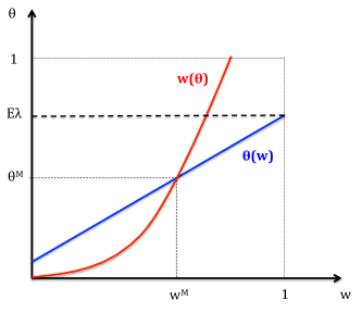
Figure 2: Equilibrium of the search model

We conclude by comparing Berk-Nash equilibria to the optimal strategy of a worker who knows the primitives, $w^{*}$. By standard arguments, $w^{*}$ is the unique solution to

$$w^{\ast}(1-\delta+\delta\overline{\gamma})=\delta(\overline{\lambda}-E[\gamma\lambda])\int_{w>w^{\ast}}\left(w-w^{\ast}\right)F(dw).$$ (8)

The only difference between equations (6) and (8) appears in the term multiplying the RHS, which captures the cost of accepting a wage offer. In the misspecified case, this term is $\delta\theta(1-\overline{\gamma})$; in the correct case, it is $\delta(\overline{\lambda}-E[\gamma\lambda])=\delta\overline{\lambda}(1-\overline{\gamma})-\delta Cov(\gamma,\lambda)$. The misspecification affects the optimal threshold in two ways. First, the misspecified agent estimates the mean of $\lambda$ incorrectly, i.e., $\theta<\overline{\lambda}$; therefore, she (incorrectly) believes that, in expectation, offers arrive with lower probability. Second, she does not realize that, because $Cov(\gamma,\lambda)<0$, she is less likely to receive an offer when fired. Both effects go in the same direction and make the option to reject and wait for the possibility of drawing a new wage offer next period less attractive for the misspecified worker. Formally, $\theta\delta(1-\overline{\gamma})<\delta\overline{\lambda}(1-\overline{\gamma})-\delta Cov(\gamma,\lambda)$ and so $w^{M}<w^{*}$.

4.3 Stochastic growth with correlated shocks

Stochastic growth models have been central to studying optimal intertemporal allocation of capital and consumption since the work of Brock and Mirman (1972). Freixas (1981) and Koulovatianos et al. (2009) assume that agents learn the distribution over productivity shocks with correctly specified models. We follow Hall (1997) and subsequent literature in incorporating shocks to both preferences and productivity, but assume that these shocks are (positively) correlated. We show that agents who fail to account for the correlation of shocks underinvest in equilibrium.

MDP. In each period $t$, an agent observes $s_{t}=(y_{t},z_{t})\in\mathbb{S}=\mathbb{R}_{+}\times\{L,H\}$, where $y_{t}$ is income from the previous period and $z_{t}$ is a current utility shock, and chooses how much income to save, $x_{t}\in\Gamma(y_{t},z_{t})=[0,y_{t}]\subseteq\mathbb{X}=\mathbb{R}_{+}$, consuming the rest. Current period utility is $\pi(y_{t},z_{t},x_{t})=z_{t}\ln(y_{t}-x_{t})$. Income next period, $y_{t+1}$, is given by

$$\ln y_{t+1}=\alpha^{*}+\beta^{*}\ln x_{t}+\varepsilon_{t},$$ (9)

where $\varepsilon_{t}=\gamma^{*}z_{t}+\xi_{t}$ is an unobserved productivity shock, $\xi_{t}\sim N(0,1)$, and $0<\delta\beta^{*}<1$, where $\delta\in[0,1)$ is the discount factor. We assume that $\gamma^{*}>0$, so that the utility and productivity shocks are positively correlated. Let $0<L<H$ and let $q\in(0,1)$ be the probability that the shock is $H$.

SMDP. The agent believes that

$$\ln y_{t+1}=\alpha+\beta\ln x_{t}+\varepsilon_{t},$$ (10)

where $\varepsilon_{t}\sim N(0,1)$ and is independent of the utility shock. For simplicity, we assume that the agent knows the distribution of the utility shock, and is uncertain about $\theta=(\alpha,\beta)\in\Theta=\mathbb{R}^{2}$. The subjective transition probability function $Q_{\theta}(y^{\prime},z^{\prime}\mid y,z,x)$ is such that $y^{\prime}$ and $z^{\prime}$ are independent, $y^{\prime}$ has a log-normal distribution with mean $\alpha+\beta\ln x$ and unit variance, and and $z^{\prime}=H$ with probability $q$. The agent has a misspecified model because she believes that the productivity and utility shocks are independent when in fact $\gamma^{*}\neq 0$.

Equilibrium. Optimality. The Bellman equation for the agent is

$$V(y,z)=\max_{0\leq x\leq y}z\ln(y-x)+\delta E\left[V(Y^{\prime},Z^{\prime})\mid x\right]$$

and it is straightforward to verify that the optimal strategy is to invest a fraction of income that depends on the utility shock and the unknown parameter $\beta$, i.e., $x=A_{z}(\beta)\cdot y$, where $A_{L}(\beta)=\frac{\delta\beta((1-q)L+qH)}{(1-\delta\beta(1-q))H+\delta\beta(1-q)}$ and $A_{H}(\beta)=\frac{\delta\beta((1-q)L+qH)}{\delta\beta qH+(1-\delta\beta q)L}<A_{L}(\beta)$. For the agent who knows the primitives, the optimal strategy is to invest fractions $A_{L}(\beta^{*})$ and $A_{H}(\beta^{*})$ in the low and high state, respectively. Since $\beta\mapsto A_{z}(\beta)$ is increasing, the equilibrium strategy of a misspecified agent can be compared to the optimal strategy by comparing the equilibrium belief about $\beta$ with the true $\beta^{*}$.

Beliefs and stationary distribution. Let $A=(A_{L},A_{H})$, with $A_{H}<A_{L}$, represent a strategy, where $A_{z}$ is the proportion of income invested given utility shock $z$. Because the agent believes that $\varepsilon_{t}$ is independent of the utility shock and normally distributed, minimizing the wKLD function is equivalent to performing an OLS regression of equation (10). Thus, for a strategy represented by $A=(A_{L},A_{H})$, the parameter value $\hat{\beta}(A)$ that minimizes wKLD is

$$\hat{\beta}(A) =\frac{Cov(\ln Y^{\prime},\ln X)}{Var(\ln X)}=\frac{Cov(\ln Y^{\prime},\ln A_{Z}Y)}{Var(\ln A_{Z}Y)}$$

$$=\beta^{*}+\gamma^{*}\frac{Cov(Z,\ln A_{Z})}{Var(\ln A_{Z})+Var(Y)}.$$

where $Cov$ and $Var$ are taken with respect to the (true) stationary distribution of $(Y,Z)$. Since $A_{H}<A_{L}$, then $Cov(Z,\ln A_{Z})<0$. Therefore, the assumption that $\gamma^{*}>0$ implies that the bias $\hat{\beta}(A)-\beta^{*}$ is negative and its magnitude depends on the strategy $A$. Intuitively, the agent invests a larger fraction of income when $z$ is low, which happens to be during times when $\varepsilon$ is also low.

Equilibrium. We establish that there exists at least one equilibrium with positive investment by showing that there is at least one fixed point of the function $\hat{\beta}(A_{L}(\beta),A_{H}(\beta))$. The function is continuous in $\beta$ and satisfies $\hat{\beta}(A_{L}(0),A_{H}(0))=\hat{\beta}(A_{L}(1/\delta),A_{H}(1/\delta))=\beta^{*}$ and $\hat{\beta}(A_{L}(\beta),A_{H}(\beta))<\beta^{*}$ for all $\beta\in(0,1/\delta)$. Then, since $\delta\beta^{*}<1$, there is at least one fixed point $\beta^{M}$, and any fixed point satisfies $\beta^{M}\in(0,\beta^{*})$. Thus, the misspecified agent underinvests in equilibrium compared to the optimal strategy. The conclusion is reversed if $\gamma^{*}<0$, illustrating how the framework provides predictions about beliefs and behavior that depend on the primitives (as opposed to simply postulating that the agent is over or under-confident about productivity).

5 Equilibrium foundation

In this section, we provide a learning foundation for the notion of Berk-Nash equilibrium of SMDPs. We fix an SMDP and assume that the agent is Bayesian and starts with a prior $\mu_{0}\in\Delta(\Theta)$ over her set of models of the world. She observes past actions and states and uses this information to update her beliefs about $\Theta$ in every period.

Definition 11.

For any $(s,x,s^{\prime})\in Gr(\Gamma)\times\mathbb{S}$, let $B(s,x,s^{\prime},\cdot):D_{s,x,s^{\prime}}\rightarrow\Delta(\Theta)$ denote the Bayesian operator: For all $A\subseteq\Theta$ Borel

$$B(s,x,s^{\prime},\mu)(A)=\frac{\int_{A}Q_{\theta}(s^{\prime}\mid s,x)\mu(d\theta)}{\int_{\Theta}Q_{\theta}(s^{\prime}\mid s,x)\mu(d\theta)}.$$ (11)

for any $\mu\in D_{s,x,s^{\prime}}$, where $D_{s,x,s^{\prime}}=\{p\in\Delta(\Theta)\colon\int_{\Theta}Q_{\theta}(s^{\prime}\mid s,x)p(d\theta)>0\}$.

Definition 12.

A Bayesian Subjective Markov Decision Process (Bayesian-SMDP) is an SMDP($Q,\mathcal{Q}_{\Theta}$) together with a prior $\mu_{0}\in\Delta(\Theta)$ and the Bayesian operator $B$ (see Definition 11). It is said to be regular if the corresponding SMDP is regular.

By the Principle of Optimality, the agent’s problem in a Bayesian-SMDP can be cast recursively as

$$W(s,\mu)=\max_{x\in\Gamma(s)}\int_{\mathbb{S}}\left\{\pi(s,x,s^{\prime})+\delta W(s^{\prime},\mu^{\prime})\right\}\bar{Q}_{\mu}(ds^{\prime}|s,x),$$ (12)

where $\bar{Q}_{\mu}=\int_{\Theta}Q_{\theta}\mu(d\theta)$, $\mu^{\prime}=B(s,x,s^{\prime},\mu)$ is next period’s belief, updated using Bayes’ rule, and $W:\mathbb{S}\times\Delta(\Theta)\rightarrow\mathbb{R}$ is the (unique) solution to the Bellman equation (12). Compared to the case where the agent knows the transition probability function, the agent’s belief about $\Theta$ is now part of the state space.

Definition 13.

A policy function is a function $f:\Delta(\Theta)\rightarrow\Sigma$ mapping beliefs into strategies (recall that a strategy is a mapping $\sigma:\mathbb{S}\rightarrow\Delta(\mathbb{X})$). For any belief $\mu\in\Delta(\Theta)$, state $s\in\mathbb{S}$, and action $x\in\mathbb{X}$, let $f(x\mid s,\mu)$ denote the probability that the agent chooses $x$ when selecting policy function $f$. A policy function $f$ is optimal for the Bayesian-SMDP if, for all $s\in\mathbb{S}$, $\mu\in\Delta(\Theta)$, and $x\in\mathbb{X}$ such that $f(x\mid s,\mu)>0$,

$$x\in\arg\max_{\hat{x}\in\Gamma(s)}\int_{\mathbb{S}}\left\{\pi(s,\hat{x},s^{\prime})+\delta W(s^{\prime},\mu^{\prime})\right\}\bar{Q}_{\mu}(ds^{\prime}|s,\hat{x}).$$

For each $\mu\in\Delta(\Theta)$, let $\bar{\Sigma}(\mu)\subseteq\Sigma$ denote the set of all strategies that are induced by a policy that is optimal, i.e.,

$$\bar{\Sigma}(\mu)=\bigl{\{}\sigma\in\Sigma:\exists\,\,\mbox{optimal }f\,\,\mbox{such that $\sigma(\cdot\mid s)=f(\cdot\mid s,\mu)$for all $s\in\mathbb{S}$}\bigr{\}}.$$

Lemma 4.

(i) There is a unique solution $W$ to the Bellman equation in (12), and it is continuous in $\mu$ for all $s\in\mathbb{S}$; (ii) The correspondence of optimal strategies $\mu\mapsto\bar{\Sigma}(\mu)$ is non-empty, compact-valued, convex-valued, and upper hemicontinuous.

Proof.

The proof is standard and relegated to the Online Appendix. ∎

Let $h^{\infty}=(s_{0},x_{0},...,s_{t},x_{t},...)$ represent the infinite history or outcome path of the dynamic optimization problem and let $\mathbb{H}^{\infty}\equiv(Gr(\Gamma))^{\infty}$ represent the space of infinite histories. For every $t$, let $\mu_{t}:\mathbb{H}^{\infty}\rightarrow\Delta(\Theta)$ denote the agent’s Bayesian beliefs, defined recursively by $\mu_{t}=B(s_{t-1},x_{t-1},s_{t},\mu_{t-1})$ whenever $\mu_{t-1}\in D_{s_{t-1},x_{t-1},s_{t}}$ (see Definition 11), and arbitrary otherwise. We assume that the agent follows some policy function $f$. In each period $t$, there is a state $s_{t}$ and a belief $\mu_{t}$, and the agent chooses a (possibly mixed) action $f(\cdot\mid s_{t},\mu_{t})\in\Delta(\mathbb{X})$. After an action $x_{t}$ is realized, the state $s_{t+1}$ is drawn from the true transition probability. The agent observes the realized action and the new state and updates her beliefs to $\mu_{t+1}$ using Bayes’ rule. The primitives of the Bayesian-SMDP (including the initial distribution over states, $q_{0}$, and the prior, $\mu_{0}\in\Delta(\Theta)$) and a policy function $f$ induce a probability distribution over $\mathbb{H}^{\infty}$ that is defined in a standard way; let $\boldsymbol{P}^{f}$ denote this probability distribution over $\mathbb{H}^{\infty}$.

We now define strategies and outcomes as random variables. For a fixed policy function $f$ and for every $t$, let $\sigma_{t}:\mathbb{H}^{\infty}\rightarrow\Sigma$ denote the strategy of the agent, defined by setting

$$\sigma_{t}(h^{\infty})=f(\cdot\mid\cdot,\mu_{t}(h^{\infty}))\in\Sigma.$$

Finally, for every $t$, let $m_{t}:\mathbb{H}^{\infty}\rightarrow\Delta(Gr(\Gamma))$ be such that, for all $t$, $h^{\infty}$, and $(s,x)\in Gr(\Gamma)$,

$$m_{t}(s,x\mid h^{\infty})=\frac{1}{t}\sum_{\tau=0}^{t}\mathbf{1}_{(s,x)}(s_{\tau},x_{\tau})$$

is the frequency of times that the outcome $(s,x)$ occurs up to time $t$.

One reasonable criteria to claim that the agent has reached a steady-state is that her strategy and the time average of outcomes converge.

Definition 14.

A strategy and probability distribution $(\sigma,m)\in\Sigma\times\Delta(Gr(\Gamma))$ is stable for a Bayesian-SMDP with prior $\mu_{0}$ and policy function $f$ if there is a set $\mathcal{H}\subseteq\mathbb{H}$ with $\mathbf{P}^{f}\left(\mathcal{H}\right)>0$ such that, for all $h^{\infty}\in\mathcal{H}$, as $t\rightarrow\infty$,

$$\sigma_{t}(h^{\infty})\rightarrow\sigma\,\,\,\,\,\mbox{and}\,\,\,\,\,m_{t}(h^{\infty})\rightarrow m.$$ (13)

If, in addition, there exists a belief $\mu^{*}$ and a subsequence $(\mu_{t(j)})_{j}$ such that,

$$\mu_{t(j)}(h^{\infty})\overset{w}{\rightarrow}\mu^{*}$$ (14)

and, for all $(s,x)\in Gr(\Gamma)$, $\mu^{*}=B(s,x,s^{\prime},\mu^{*})$ for all $s^{\prime}\in\mathbb{S}$ such that $\bar{Q}_{\mu^{*}}(s^{\prime}\mid s,x)>0$, then $(\sigma,m)$ is called stable with exhaustive learning.

Condition (13) requires that strategies and the time frequency of outcomes stabilize. By compactness, there exists a subsequence of beliefs that converges. The additional requirement of exhaustive learning says that the limit point of one of the subsequences, $\mu^{*}$, is perceived to be a fixed point of the Bayesian operator, implying that no matter what state and strategy the agent contemplates, she does not expect her belief to change. Thus, the agent believes that all learning possibilities are exhausted under $\mu^{*}$. The condition, however, does not imply that the agent has correct beliefs in steady state.

The next result establishes that, if the time average of outcomes stabilize to $m$, then beliefs become increasingly concentrated on $\Theta_{Q}(m)$.

Lemma 5.

Consider a regular Bayesian-SMDP with true transition probability function $Q$, full-support prior $\mu_{0}\in\Delta(\Theta)$, and policy function $f$. Suppose that $(m_{t})_{t}$ converges to $m$ for all histories in a set $\mathcal{H}\subseteq\mathbb{H}$ such that $\mathbf{P}^{f}\left(\mathcal{H}\right)>0$. Then, for all open sets $U\supseteq\Theta_{Q}(m)$,

$$\lim_{t\rightarrow\infty}\mu_{t}\left(U\right)=1$$

$\mathbf{P}^{f}$-a.s. in $\mathcal{H}$.

Proof.

See the Appendix. ∎

The proof of Lemma 5 clarifies the origin of the wKLD function in the definition of Berk-Nash equilibrium. The proof adapts the proof of Lemma 2 by Esponda and Pouzo (2016) to dynamic environments. Lemma 5 extends results from the statistics of misspecified learning (Berk (1966), Bunke and Milhaud (1998), Shalizi (2009)) by considering a setting where agents learn from data that is endogenously generated by their own actions in a Markovian setting.

The following result provides a learning foundation for the notion of Berk-Nash equilibrium of an SMDP.

Theorem 2.

There exists $\bar{\delta}\in[0,1]$ such that:

(i) for all $\delta\leq\bar{\delta}$, if $(\sigma,m)$ is stable for a regular Bayesian-SMDP with full-support prior $\mu_{0}$ and policy function $f$ that is optimal, then $(\sigma,m)$ is a Berk-Nash equilibrium of the SMDP.

(ii) for all $\delta>\bar{\delta}$, if $(\sigma,m)$ is stable with exhaustive learning for a regular Bayesian-SMDP with full-support prior $\mu_{0}$ and policy function $f$ that is optimal, then $(\sigma,m)$ is a Berk-Nash equilibrium of the SMDP.

Proof.

See the Appendix. ∎

Theorem 2 provides a learning justification for Berk-Nash equilibrium. The main idea behind the proof is as follows. We can always find a subsequence of posteriors that converges to some $\mu^{*}$ and, by Lemma 5 and the fact that behavior converges to $\sigma$, it follows that $\sigma$ must solve the dynamic optimization problem for beliefs converging to $\mu^{*}\in\Theta_{Q}(m)$. In addition, by convergence of $\sigma_{t}$ to $\sigma$ and continuity of the transition kernel $\sigma\mapsto M_{\sigma,Q}$, an application of the martingale convergence theorem implies that $m_{t}$ is asymptotically equal to $M_{\sigma,Q}[m_{t}]$. This fact, linearity of the operator $M_{\sigma,Q}[\cdot]$, and convergence of $m_{t}$ to $m$ then imply that $m$ is an invariant distribution given $\sigma$.

The proof concludes by showing that $\sigma$ not only solves the optimization problem for beliefs converging to $\mu^{*}$ but also solves the MDP, where the belief is forever fixed at $\mu^{*}$. This is true, of course, if the agent is sufficiently impatient, which explains why part (i) of Theorem 2 holds. For sufficiently patient agents, the result relies on the assumption that the steady state satisfies exhaustive learning. We now illustrate and discuss the role of this assumption.

example. At the initial period, a risk-neutral agent has four investment choices: A, B, S, and O. Action A pays $1-\theta^{*}$, action B pays $\theta^{*}$, and action S pays a safe payoff of 2/3 in the initial period, where $\theta^{*}\in\{0,1\}$. For any of these three choices, the decision problem ends there and the agent makes a payoff of zero in all future periods. Action O gives the agent a payoff of $-1/3$ in the initial period and the option to make an investment next period, where there are two possible states, $s_{A}$ and $s_{B}$. State $s_{A}$ is realized if $\theta^{*}=1$ and state $s_{B}$ is realized if $\theta^{*}=0$. In each of these states, the agent can choose to make a risky investment or a safe investment. The safe investment gives a payoff of 2/3 in both states, and a subsequent payoff of zero in all future periods. The risky investment gives the agent a payoff that is thrice the payoff she would have gotten from choice A, that is, $3(1-\theta^{*})$, if the state is $s_{A}$, and it gives the agent thrice the payoff she would have gotten from choice B, that is, $3\theta^{*}$, if the state is $s_{B}$; the payoff is zero is all future periods.

Suppose that the agent knows all the primitives except the value of $\theta^{*}$. Let $\Theta=\{0,1\}$; in particular, the SMDP is correctly specified. We now show that, in any Berk-Nash equilibrium, a sufficiently patient agent never chooses the safe action S: Let $\mu\in[0,1]$ denote the agent’s equilibrium belief about the probability that $\theta^{*}=1$. For action S to be preferred to A and B, it must be the case that $\mu\in[1/3,2/3]$. But, for a fixed $\mu$, the perceived benefit from action O is

$$-\frac{1}{3}+\delta\left(\mu V_{\bar{Q}_{\mu}}(s_{A})+(1-\mu)V_{\bar{Q}_{\mu}}(s_{B})\right) =-\frac{1}{3}+\delta\left(\mu\max\{\frac{2}{3},3(1-\mu)\}+(1-\mu)\max\{\frac{2}{3},3\mu\}\right)$$

$$\geq-\frac{1}{3}+\delta 6\mu(1-\mu),$$

which is strictly higher than 2/3, the payoff from action S, for all $\mu\in[1/3,2/3]$ provided that $\delta>\bar{\delta}=3/4$. Thus, for a sufficiently patient agent, there is no belief that makes action S optimal and, therefore, S is not chosen in any Berk-Nash equilibrium.

Now consider a Bayesian agent who starts with a prior $\mu_{0}=\Pr(\theta=1)\in(0,1)$ and updates her belief. The value of action O is

$$-\frac{1}{3}+\delta\left(\mu_{0}W(s_{A},1)+(1-\mu_{0})W(s_{B},0)\right)=-\frac{1}{3}+\delta\frac{2}{3}<\frac{2}{3}$$

because $W(s_{A},1)=W(s_{B},0)=2/3$. In other words, the agent realizes that if the state $s_{A}$ is realized, then she will update her belief to $\mu_{1}=1$, which implies that the safe investment is optimal in state $s_{A}$; a similar argument holds for state $s_{B}$. She then finds it optimal to choose action A if $\mu_{0}\leq 1/3$, B if $\mu_{0}\geq 2/3$, and S if $\mu_{0}\in[1/3,2/3]$. In particular, choosing S is a steady state outcome for some priors, although it is not chosen in any Berk-Nash equilibrium if the agent is sufficiently patient. The belief supporting S, however, does not satisfy exhaustive learning, since the agent believes that any other action would completely reveal all uncertainty. $\square$

More generally, the failure of a steady state to be a Berk-Nash equilibrium if the agent is sufficiently patient occurs because the value of experimentation can be negative. To see this point, let the value of experimentation for action $x$ at state $s$ when the agent’s belief is $\mu$ be

$$ValueExp(s,x;\mu)\equiv E_{\bar{Q}_{\mu}(\cdot\mid s,x)}\left[W(S^{\prime},B(s,x,S^{\prime},\mu))\right]-E_{\bar{Q}_{\mu}(\cdot\mid s,x)}\bigl{[}V_{\bar{Q}_{\mu}}(S^{\prime})\bigr{]}.$$

This expression is the difference between the value when the agent updates her prior $\mu$ and the value when the agent has a fixed belief $\mu$. An agent who does not account for future changes in beliefs may end up choosing an action with a negative value of experimentation that is actually suboptimal when accounting for changes in beliefs.

In the previous example, the value of experimentation for action O given $\mu$ is

$$\left(\mu W(s_{A},1)+(1-\mu)W(s_{B},0)\right)-\left(\mu V_{\bar{Q}_{\mu}}(s_{A})+(1-\mu)V_{\bar{Q}_{\mu}}(s_{B})\right),$$

which reduces to $2/3-6\mu(1-\mu)$ and is negative for the values of $\mu$ that make S better than A and B. Thus, it is possible for action O to be optimal if the agent does not account for changes in beliefs, but suboptimal if she does.

We now discuss specifically how the property of exhaustive learning is used in the proof of Theorem 2. We call an action a steady-state action if it is in the support of a stable strategy and we call it a non steady-state action otherwise. A key step is to show that, if a steady-state action is better than a non steady-state action when beliefs are updated, it will also be better when beliefs are fixed. This is true provided that there is zero value of experimenting in steady state, which is guaranteed by exhaustive learning. If instead of exhaustive learning we were to simply require weak identification, there would be no value of experimentation for steady-state actions. The concern, illustrated by the previous example, is that the value of experimentation can be negative for a non steady-state action. Therefore, a non steady-state action could be suboptimal in the problem where the belief is updated but optimal in the problem where the belief is not updated (and so the negative value of experimentation is not taken into account). As shown by Esponda and Pouzo (2016), this concern does not arise in static settings, where the only state variable is a belief. The reason is that the convexity of the value function and the martingale property of Bayesian beliefs imply that the value of experimentation is always nonnegative.

We conclude with additional remarks about Theorem 2.

Remark 3.

Discount factor: In the proof of Theorem 2, we provide an exact value for $\bar{\delta}$ as a function of primitives. This bound, however, may not be sharp. As illustrated by the above example, to compute a sharp bound we would have to solve the dynamic optimization problem with learning, which is precisely what we are trying to avoid by focusing on Berk-Nash equilibrium.

Convergence: Theorem 2 does not imply that behavior will necessarily stabilize in an SMDP. In fact, it is well known from the theory of Markov chains that, even if no decisions affect the relevant transitions, outcomes need not stabilize without further assumptions. So one cannot hope to have general statements regarding convergence of outcomes—this is also true, for example, in the related context of learning to play Nash equilibrium in games. Thus, the theorem leaves open the question of convergence in specific settings, a question that requires other tools (e.g., stochastic approximation) and is best tackled by explicitly studying the dynamics of specific classes of environments (see the references in the introduction).

Mixed strategies: Theorem 2 also raises the question of how a mixed strategy could ever become stable, given that, in general it is unlikely that agents will hold beliefs that make them exactly indifferent at any point in time. Fudenberg and Kreps (1993) asked the same question in the context of learning to play mixed strategy Nash equilibria, and answered it by adding small payoff perturbations a la Harsanyi (1973): Agents do not actually mix; instead, every period their payoffs are subject to small perturbations, and what we call the mixed strategy is simply the probability distribution generated by playing pure strategies and integrating over the payoff perturbations. We followed this approach in the paper that introduced Berk-Nash equilibrium in static contexts (Esponda and Pouzo, 2016). The same idea applies here, but we omit payoff perturbations to reduce the notational burden.

6 Equilibrium refinements

Theorem 2 implies that, for sufficiently patient players, we should be interested in the following refinement of Berk-Nash equilibrium.

Definition 15.

A strategy and probability distribution $(\sigma,m)\in\Sigma\times\Delta(Gr(\Gamma))$ is a Berk-Nash equilibrium with exhaustive learning of the SMDP if it is a Berk-Nash equilibrium that is supported by a belief $\mu^{*}\in\Delta(\Theta)$ such that, for all $(s,x)\in Gr(\Gamma)$,

$$\mu^{*}=B(s,x,s^{\prime},\mu^{*})$$

for all $s^{\prime}\in\mathbb{S}$ such that $\bar{Q}_{\mu^{*}}(s^{\prime}\mid s,x)>0$.

In an equilibrium with exhaustive learning, there is a supporting belief that is perceived to be a fixed point of the Bayesian operator, implying that no matter what state and strategy the agent contemplates, she does not expect her belief to change. The requirement of exhaustive learning does not imply robustness to experimentation. For example, in the monopoly problem studied in Section 4.1, choosing low price with probability 1 is an equilibrium with exhausted learning which is supported by the belief that, with probability 1, $\theta_{L}^{*}=0$. We rule out equilibria that are not robust to experimentation by introducing a further refinement.

Definition 16.

An $\varepsilon$-perturbed SMDP is an SMDP wherein strategies are restricted to belong to

$$\Sigma^{\varepsilon}=\left\{\sigma\in\Sigma:\sigma(x\mid s)\geq\varepsilon\,\,\mbox{for all $(s,x)\in Gr(\Gamma)$}\right\}.$$

Definition 17.

A strategy and probability distribution $(\sigma,m)\in\Sigma\times\Delta(Gr(\Gamma))$ is a perfect Berk-Nash equilibrium of an SMDP if there exists a sequence $(\sigma^{\varepsilon},m^{\varepsilon})_{\varepsilon>0}$ of Berk-Nash equilibria with exhaustive learning of the $\varepsilon$-perturbed SMDP that converges to $(\sigma,m)$ as $\varepsilon\rightarrow 0$.

Selten (1975) introduced the idea of perfection in extensive-form games. By itself, however, perfection does not guarantee that all $(s,x)\in Gr(\Gamma)$ are reached in an MDP. The next property guarantees that all states can be reached when the agent chooses all strategies with positive probability.

Definition 18.

An MDP($Q$) satisfies full communication if, for all $s_{0},s^{\prime}\in\mathbb{S}$, there exist finite sequences $(s_{1},...,s_{n})$ and $(x_{0},x_{1},...,x_{n})$ such that $(s_{i},x_{i})\in Gr(\Gamma)$ for all $i=0,1,...,n$ and

$$Q(s^{\prime}\mid s_{n},x_{n})Q(s_{n}\mid s_{n-1},x_{n-1})...Q(s_{1}\mid s_{0},x_{0})>0.$$

An SMDP satisfies full communication if the corresponding MDP satisfies it.

Full communication is standard in the theory of MDPs and holds in all of the examples in Section 4. It guarantees that there is a single recurrent class of states for all $\varepsilon$-perturbed environments. In cases where it does not hold and there is more than one recurrent class of states, one can still apply the following results by focusing on one of the recurrent classes and ignoring the rest as long as the agent correctly believes that she cannot go from one recurrent class to the other.

Full communication guarantees that there are no off-equilibrium outcomes in a perturbed SMDP. It does not, however, rule out the desire for experimentation on the equilibrium path. We rule out the latter by requiring weak identification.

Proposition 2.

Suppose that an SMDP is weakly identified, $\varepsilon$-perturbed, and satisfies full communication.

(i) If the SMDP is regular and if $(\sigma,m)$ is stable for the Bayesian-SMDP, it is also stable with exhaustive learning.

(ii) If $(\sigma,m)$ is a Berk-Nash equilibrium, it is also a Berk-Nash equilibrium with exhaustive learning.

Proof.

See the Appendix. ∎

Proposition 2 provides conditions such that a steady state satisfies exhaustive learning and a Berk-Nash equilibrium can be supported by a belief that satisfies the exhaustive learning condition. Under these conditions, we can find equilibria that are robust to experimentation, i.e., perfect equilibria, by considering perturbed environments and taking the perturbations to zero (see the examples in Section 4).

The next proposition shows that perfect Berk-Nash is a refinement of Berk-Nash with exhaustive learning. As illustrated by the monopoly example in Section 4.1, it is a strict refinement.

Proposition 3.

Any perfect Berk-Nash equilibrium of a regular SMDP is a Berk-Nash equilibrium with exhaustive learning.

Proof.

See the Appendix. ∎

We conclude by showing existence of perfect Berk-Nash equilibrium (hence, of Berk-Nash equilibrium with exhaustive learning, by Proposition 3).

Theorem 3.

For any regular SMDP that is weakly identified and satisfies full communication, there exists a perfect Berk-Nash equilibrium.

Proof.

See the Appendix. ∎

7 Conclusion

We studied Markov decision processes where the agent has a prior over a set of possible transition probability functions and updates her beliefs using Bayes’ rule. This problem is relevant in many economic settings but usually not amenable to analysis. We propose to make it more tractable by studying asymptotic beliefs and behavior. The answer to the question “Can the steady state of a Bayesian-SMDP be characterized by reference to an MDP with fixed beliefs?” is a qualified yes. If the agent is sufficiently impatient, it suffices to focus on the set of Berk-Nash equilibria. If, on the other hand, the agent is sufficiently patient and we are interested in steady states with exhaustive learning, then these steady states are characterized by the notion of Berk-Nash equilibrium with exhaustive learning. Finally, if we are interested on equilibria that are robust to experimentation, we can restrict attention to the set of perfect Berk-Nash equilibria.

Our results hold for both the correctly-specified and misspecified cases, and we are not aware of any prior general results for either of these cases. For the correctly-specified case, our results can justify the common assumption in the literature that the agent knows the transition probability function provided that strong identification holds (or that there is weak identification and one is interested in equilibria that are robust to experimentation). In the misspecified case, our results significantly expand the range of possible applications.

Appendix

Proof of Lemma 2. $I_{Q}(\sigma)$ is nonempty: $M_{\sigma,Q}$ is a linear (hence continuous) self-map on a convex and compact subset of an Euclidean space (the set of probability distributions over the finite set $Gr(\Gamma)$); hence, Brower’s theorem implies existence of a fixed point.

$I_{Q}(\sigma)$ is convex valued: For all $\alpha\in[0,1]$ and $m_{1},m_{2}\in\Delta(Gr(\Gamma))$, $\alpha M_{\sigma,Q}[m_{1}]+(1-\alpha)M_{\sigma,Q}[m_{2}]=M_{\sigma,Q}[\alpha m_{1}+(1-\alpha)m_{2}]$. Thus, if $m_{1}=M_{\sigma,Q}[m_{1}]$ and $m_{2}=M_{\sigma,Q}[m_{2}]$, then $\alpha m_{1}+(1-\alpha)m_{2}=M_{\sigma,Q}[\alpha m_{1}+(1-\alpha)m_{2}]$.

$I_{Q}(\sigma)$ is upper hemicontinuous and compact valued: Fix any sequence $(\sigma_{n},m_{n})_{n}$ in $\Sigma\times\Delta(Gr(\Gamma))$ such that $\lim_{n\rightarrow\infty}(\sigma_{n},m_{n})=(\sigma,m)$ and such that $m_{n}\in I_{Q}(\sigma_{n})$ for all $n$. Since $M_{\sigma_{n},Q}[m_{n}]=m_{n}$, $||m-M_{\sigma,Q}[m]||\leq||m-m_{n}||+||M_{\sigma_{n},Q}[m_{n}-m]||+||M_{\sigma_{n},Q}[m]-M_{\sigma,Q}[m]||$. The first term in the RHS vanishes by the hypothesis. The second term satisfies $||M_{\sigma_{n},Q}[m_{n}-m]||\leq||M_{\sigma_{n},Q}||\times||m_{n}-m||$ and also vanishes. For the third term, note that $\sigma\mapsto M_{\sigma,Q}[m]$ is a linear mapping and $\sup_{\sigma}||M_{\sigma,Q}[m]||\leq\max_{s^{\prime}}|\sum_{(s,x)\in Gr(\Gamma)}Q(s^{\prime}\mid s,x)m(s,x)|<\infty$. Thus $||M_{\sigma_{n},Q}[m]-M_{\sigma,Q}[m]||\leq K\times||\sigma_{n}-\sigma||$ for some $K<\infty$ , and so it also vanishes. Therefore, $m=M_{\sigma,Q}[m]$; thus, $I_{Q}(\cdot)$ has a closed graph and so $I_{Q}(\sigma)$ is a closed set. Compactness of $I_{Q}(\sigma)$ follows from compactness of $\Delta(Gr(\Gamma))$. Therefore, $I_{Q}(\cdot)$ is upper hemicontinuous (see Aliprantis and Border (2006), Theorem 17.11). $\square$

The proof of Lemma 3 relies on the following claim. The proofs of Claims A, B, and C in this appendix appear in the Online Appendix .

Claim A. (i) For any regular SMDP, there exists $\theta^{*}\in\Theta$ and $K<\infty$ such that, for all $m\in\Delta(Gr(\Gamma))$, $K_{Q}(m,\theta^{*})\leq K$. (ii) Fix any $\theta\in\Theta$ and a sequence $(m_{n})_{n}$ in $\Delta(Gr(\Gamma))$ such that $Q_{\theta}(s^{\prime}\mid s,x)>0$ for all $(s^{\prime},s,x)\in\mathbb{S}\times Gr(\Gamma)$ such that $Q(s^{\prime}\mid s,x)>0$ and $\lim_{n\rightarrow\infty}m_{n}=m$. Then $\lim_{n\rightarrow\infty}K_{Q}(m_{n},\theta)=K_{Q}(m,\theta)$. (iii) $K_{Q}$ is (jointly) lower semicontinuous: Fix any $(m_{n})_{n}$ and $(\theta_{n})_{n}$ such that $\lim_{n\rightarrow\infty}m_{n}=m$ and $\lim_{n\rightarrow\infty}\theta_{n}=\theta$. Then $\liminf_{n\rightarrow\infty}K_{Q}(m_{n},\theta_{n})\geq K_{Q}(m,\theta)$.

Proof of Lemma 3. (i) By Jensen’s inequality and strict concavity of $\ln(\cdot)$, $K_{Q}(m,\theta)\geq-\sum_{(s,x)\in Gr(\Gamma)}\ln(E_{Q(\cdot\mid s,x)}[\frac{Q_{\theta}(S^{\prime}\mid s,x)}{Q(S^{\prime}\mid s,x)}])m(s,x)=0$, with equality if and only if $Q_{\theta}(\cdot\mid s,x)=Q_{\theta}(\cdot\mid s,x)$ for all $(s,x)$ such that $m(s,x)>0$.

(ii) $\Theta_{Q}(m)$ is nonempty: By Claim A(i), there exists $K<\infty$ such that the minimizers are in the constraint set $\{\theta\in\Theta:K_{Q}(m,\theta)\leq K\}$. Because $K_{Q}(m,\cdot)$ is continuous over a compact set, a minimum exists.

$\Theta_{Q}(\cdot)$ is uhc and compact valued: Fix any $(m_{n})_{n}$ and $(\theta_{n})_{n}$ such that $\lim_{n\rightarrow\infty}m_{n}=m$, $\lim_{n\rightarrow\infty}\theta_{n}=\theta$, and $\theta_{n}\in\Theta_{Q}(m_{n})$ for all $n$. We establish that $\theta\in\Theta_{Q}(m)$ (so that $\Theta(\cdot)$ has a closed graph and, by compactness of $\Theta$, it is uhc). Suppose, in order to obtain a contradiction, that $\theta\notin\Theta_{Q}(m)$. Then, by Claim A(i), there exists $\hat{\theta}\in\Theta$ and $\varepsilon>0$ such that $K_{Q}(m,\hat{\theta})\leq K_{Q}(m,\theta)-3\varepsilon$ and $K_{Q}(m,\hat{\theta})<\infty$. By regularity, there exists $(\hat{\theta}_{j})_{j}$ with $\lim_{j\rightarrow\infty}\hat{\theta}_{j}=\hat{\theta}$ and, for all $j$, $Q_{\hat{\theta}_{j}}(s^{\prime}\mid s,x)>0$ for all $(s^{\prime},s,x)\in\mathbb{S}^{2}\times\mathbb{X}$ such that $Q(s^{\prime}\mid s,x)>0$. We will show that there is an element of the sequence, $\hat{\theta}_{J}$, that “does better” than $\theta_{n}$ given $m_{n}$, which is a contradiction. Because $K_{Q}(m,\hat{\theta})<\infty$, continuity of $K_{Q}(m,\cdot)$ implies that there exists $J$ large enough such that $\left|K_{Q}(m,\hat{\theta}_{J})-K_{Q}(m,\hat{\theta})\right|\leq\varepsilon/2$. Moreover, Claim A(ii) applied to $\theta=\hat{\theta}_{J}$ implies that there exists $N_{\varepsilon,J}$ such that, for all $n\geq N_{\varepsilon,J}$, $\left|K_{Q}(m_{n},\hat{\theta}_{J})-K_{Q}(m,\hat{\theta}_{J})\right|\leq\varepsilon/2$. Thus, for all $n\geq N_{\varepsilon,J}$, $\bigl{|}K_{Q}(m_{n},\hat{\theta}_{J})-K_{Q}(m,\hat{\theta})\bigr{|}\leq\bigl{|}K_{Q}(m_{n},\hat{\theta}_{J})-K_{Q}(m,\hat{\theta}_{J})\bigr{|}+\bigl{|}K_{Q}(m,\hat{\theta}_{J})-K_{Q}(m,\hat{\theta})\bigr{|}\leq\varepsilon$ and, therefore,

$$K_{Q}(m_{n},\hat{\theta}_{J})\leq K_{Q}(m,\hat{\theta})+\varepsilon\leq K_{Q}(m,\theta)-2\varepsilon.$$ (15)

Suppose $K_{Q}(m,\theta)<\infty$. By Claim A(iii), there exists $n_{\varepsilon}\geq N_{\varepsilon,J}$ such that $K_{Q}(m_{n_{\varepsilon}},\theta_{n_{\varepsilon}})\geq K_{Q}(m,\theta)-\varepsilon$. This result, together with (15), implies that $K_{Q}(m_{n_{\varepsilon}},\hat{\theta}_{J})\leq K_{Q}(m_{n_{\varepsilon}},\theta_{n_{\varepsilon}})-\varepsilon$. But this contradicts $\theta_{n_{\varepsilon}}\in\Theta_{Q}(m_{n_{\varepsilon}})$. Finally, if $K_{Q}(m,\theta)=\infty$, Claim A(iii) implies that there exists $n_{\varepsilon}\geq N_{\varepsilon,J}$ such that $K_{Q}(m_{n_{\varepsilon}},\theta_{n_{\varepsilon}})\geq 2K$, where $K$ is the bound defined in Claim A(i). But this also contradicts $\theta_{n_{\varepsilon}}\in\Theta_{Q}(m_{n_{\varepsilon}})$. Thus, $\Theta_{Q}(\cdot)$ has a closed graph, and so $\Theta_{Q}(m)$ is a closed set. Compactness of $\Theta_{Q}(m)$ follows from compactness of $\Theta$. Therefore, $\Theta_{Q}(\cdot)$ is upper hemicontinuous (see Aliprantis and Border (2006), Theorem 17.11). $\square$

Proof of Theorem 1. Let $\mathbb{W}=\Sigma\times\Delta(Gr(\Gamma))\times\Delta(\Theta)$ and endow it with the product topology (given by the Euclidean one for $\Sigma\times\Delta(Gr(\Gamma))$ and the weak topology for $\Delta(\Theta)$). Clearly, $\mathbb{W}\neq\{\emptyset\}$. Since $\Theta$ is compact, $\Delta(\Theta)$ is compact under the weak topology; $\Sigma$ and $\Delta(Gr(\Gamma))$ are also compact. Thus by Tychonoff’s theorem (see Aliprantis and Border (2006)), $\mathbb{W}$ is compact under the product topology. $\mathbb{W}$ is also convex. Finally, $\mathbb{W}\subseteq\mathbb{M}^{2}\times rca(\Theta)$ where $\mathbb{M}$ is the space of $|\mathbb{S}|\times|\mathbb{X}|$ real-valued matrices and $rca(\Theta)$ is the space of regular Borel signed measures endowed with the weak topology. The space $\mathbb{M}^{2}\times rca(\Theta)$ is locally convex with a family of seminorms $\{(\sigma,m,\mu)\mapsto p_{f}(\sigma,m,\mu)=||(\sigma,m)||+|\int_{\Omega}f(x)\mu(dx)|\colon\mbox{\text{ }}f\in\mathbb{C}(\Omega)\}$ ($\mathbb{C}(\Omega)$ is the space of real-valued continuous and bounded functions and $||.||$ is understood as the spectral norm). Also, we observe that $(\sigma,m,\mu)=0$ iff $p_{f}(\sigma,m,\mu)=0$ for all $f\in\mathbb{C}(\Omega)$, thus $\mathbb{M}^{2}\times rca(\Theta)$ is also Hausdorff.

Let $\mathcal{T}:\mathbb{W}\rightarrow 2^{\mathbb{W}}$ be such that $\mathcal{T}(\sigma,m,\mu)=\Sigma(\bar{Q}_{\mu})\times I_{Q}(\sigma)\times\Delta(\Theta_{Q}(m))$. Note that if $(\sigma^{*},m^{*},\mu^{*})$ is a fixed point of $\mathcal{T}$, then $m^{*}$ is a Berk-Nash equilibrium. By Lemma 1, $\Sigma(\cdot)$ is nonempty, convex valued, compact valued, and upper hemicontinuous. Thus, for every $\mu\in\Delta(\Theta)$, $\Sigma(\bar{Q}_{\mu})$ is nonempty, convex valued, and compact valued. Also, because $Q_{\theta}$ is continuous in $\theta$ (by regularity assumption), then $\bar{Q}_{\mu}$ is continuous (under the weak topology) in $\mu$. Since $Q\mapsto\Sigma(Q)$ is upper hemicontinuous, then $\Sigma(\bar{Q}_{\mu})$ is also upper hemicontinuous as a function of $\mu$. By Lemma 2, $I_{Q}(\cdot)$ is nonempty, convex valued, compact valued and upper hemicontinuous. By Lemma 3 and the regularity condition, the correspondence $\Theta_{Q}(\cdot)$ is nonempty, compact valued, and upper hemicontinuous; hence, the correspondence $\Delta(\Theta_{Q}(\cdot))$ is nonempty, upper hemicontinuous (see Aliprantis and Border (2006), Theorem 17.13), compact valued (see Aliprantis and Border (2006), Theorem 15.11) and, trivially, convex valued. Thus, the correspondence $\mathcal{T}$ is nonempty, convex valued, compact valued (by Tychonoff’s Theorem), and upper hemicontinuous (see Aliprantis and Border (2006), Theorem 17.28) under the product topology; hence, it has a closed graph (see Aliprantis and Border (2006), Theorem 17.11). Since $\mathbb{W}$ is a nonempty compact convex subset of a locally Hausdorff space, then there exists a fixed point of $\mathcal{T}$ by the Kakutani-Fan-Glicksberg theorem (see Aliprantis and Border (2006), Corollary 17.55). $\square$

For the proof of Lemma 5, we rely on the following definitions and Claim. Let $K^{\ast}(m)=\inf_{\theta\in\Theta}K_{Q}(m,\theta)$ and let $\hat{\Theta}\subseteq\Theta$ be a dense set such that, for all $\theta\in\hat{\Theta}$, $Q_{\theta}(s^{\prime}\mid s,x)>0$ for all $(s^{\prime},s,x)\in\mathbb{S}\times Gr(\Gamma)$ such that $Q(s^{\prime}\mid s,x)>0$. Existence of such a set $\hat{\Theta}$ follows from the regularity assumption.

Claim B. Suppose $\lim_{t\rightarrow\infty}\left\|m_{t}-m\right\|=0$ a.s.-$\mathbf{P}^{f}$ . Then: (i) For all $\theta\in\hat{\Theta}$,

$$\lim_{t\rightarrow\infty}t^{-1}\sum_{\tau=1}^{t}\log\frac{Q(s_{\tau}|s_{\tau-1},x_{\tau-1})}{Q_{\theta}(s_{\tau}|s_{\tau-1},x_{\tau-1})}=\sum_{(s,x)\in Gr(\Gamma)}E_{Q(\cdot|s,x)}\Bigl{[}\log\frac{Q(S^{\prime}|s,x)}{Q_{\theta}(S^{\prime}|s,x)}\Bigr{]}m(s,x)$$

a.s.-$\mathbf{P}^{f}$. (ii) For $\mathbf{P}^{f}$-almost all $h^{\infty}\in\mathbb{H}^{\infty}$ and for any $\epsilon>0$ and $\alpha=(\inf_{\Theta\colon d_{m}(\theta)\geq\epsilon}K_{Q}(m,\theta)-K^{\ast}(m))/3$, there exists $T$ such that, for all $t\geq T$,

$$t^{-1}\sum_{\tau=1}^{t}\log\frac{Q(s_{\tau}|s_{\tau-1},x_{\tau-1})}{Q_{\theta}(s_{\tau}|s_{\tau-1},x_{\tau-1})}\geq K^{\ast}(m)+\frac{3}{2}\alpha$$

for all $\theta\in\{\Theta\colon d_{m}(\theta)\geq\epsilon\}$, where $d_{m}(\theta)=\inf_{\tilde{\theta}\in\Theta_{Q}(m)}||\theta-\tilde{\theta}||$.

Proof of Lemma 5. It suffices to show that $\lim_{t\rightarrow\infty}\int_{\Theta}d_{m}(\theta)\mu_{t}(d\theta)=0$ a.s.-$\mathbf{P}^{f}$ over $\mathcal{H}$. Let $K^{\ast}(m)\equiv K_{Q}(m,\Theta_{Q}(m))$. For any $\eta>0$ let $\Theta_{\eta}(m)=\left\{\theta\in\Theta:d_{m}(\theta)<\eta\right\}$, and $\hat{\Theta}_{\eta}(m)=\hat{\Theta}\cap\Theta_{\eta}(m)$ (the set $\hat{\Theta}$ is defined in condition 3 of Definition 6, i.e., regularity). We now show that $\mu_{0}(\hat{\Theta}_{\eta}(m))>0$. By Lemma 3, $\Theta_{Q}(m)$ is nonempty. By denseness of $\hat{\Theta}$, $\hat{\Theta}_{\eta}(m)$ is nonempty. Nonemptiness and continuity of $\theta\mapsto Q_{\theta}$, imply that there exists a non-empty open set $U\subseteq\hat{\Theta}_{\eta}(m)$. By full support, $\mu_{0}(\hat{\Theta}_{\eta}(m))>0$. Also, observe that for any $\epsilon>0$, $\{\Theta\colon d_{m}(\theta)\geq\epsilon\}$ is compact. This follows from compactness of $\Theta$ and continuity of $\theta\mapsto d_{m}(\theta)$ (which follows by Lemma 3 and an application of the Theorem of the Maximum). Compactness of $\{\Theta\colon d_{m}(\theta)\geq\epsilon\}$ and lower semi-continuity of $\theta\mapsto K_{Q}(m,\theta)$ (see Claim A(iii)) imply that $\inf_{\Theta\colon d_{m}(\theta)\geq\epsilon}K_{Q}(m,\theta)=\min_{\Theta\colon d_{m}(\theta)\geq\epsilon}K_{Q}(m,\theta)>K^{\ast}(m)$. Let $\alpha\equiv(\min_{\Theta\colon d_{m}(\theta)\geq\epsilon}K_{Q}(m,\theta)-K^{\ast}(m))/3>0$. Also, let $\eta>0$ be chosen such that $K_{Q}(m,\theta)\leq K^{\ast}(m)+0.25\alpha$ for all $\theta\in\Theta_{\eta}(m)$ (such $\eta$ always exists by continuity of $\theta\mapsto K_{Q}(m,\theta)$).

Let $\mathcal{H}_{1}$ be the subset of $\mathcal{H}$ for which the statements in Claim B hold; note that $\mathbf{P}^{f}\left(\mathcal{H}\setminus\mathcal{H}_{1}\right)=0$. Henceforth, fix $h^{\infty}\in\mathcal{H}_{1}$; we omit $h^{\infty}$ from the notation to ease the notational burden. By simple algebra and the fact that $d_{m}$ is bounded in $\Theta$, it follows that, for all $\epsilon>0$ and some finite $C>0$,

$$\int_{\Theta}d_{m}(\theta)\mu_{t}(d\theta) =\frac{\int_{\Theta}d_{m}(\theta)Q_{\theta}(s_{t}\mid s_{t-1},x_{t-1})\mu_{t-1}(d\theta)}{\int_{\Theta}Q_{\theta}(s_{t}\mid s_{t-1},x_{t-1})\mu_{t-1}(d\theta)}=\frac{\int_{\Theta}d_{m}(\theta)Z_{t}(\theta)\mu_{0}(d\theta)}{\int_{\Theta}Z_{t}(\theta)\mu_{0}(d\theta)}$$

$$\leq\epsilon+C\frac{\int_{\left\{\Theta\colon d_{m}(\theta)\geq\epsilon\right\}}Z_{t}(\theta)\mu_{0}(d\theta)}{\int_{\hat{\Theta}_{\eta}(m)}Z_{t}(\theta)\mu_{0}(d\theta)}\equiv\epsilon+C\frac{A_{t}(\epsilon)}{B_{t}(\eta)}.$$

where $Z_{t}(\theta)\equiv\prod_{\tau=1}^{t}\frac{Q_{\theta}(s_{\tau}|s_{\tau-1},x_{\tau-1})}{Q(s_{\tau}|s_{\tau-1},x_{\tau-1})}=\exp\left\{-\sum_{\tau=1}^{t}\log\left(\frac{Q(s_{\tau}|s_{\tau-1},x_{\tau-1})}{Q_{\theta}(s_{\tau}|s_{\tau-1},x_{\tau-1})}\right)\right\}$. Hence, it suffices to show that

$$\limsup_{t\rightarrow\infty}\left\{\exp\left\{t\left(K^{\ast}(m)+0.5\alpha\right)\right\}A_{t}(\epsilon)\right\}=0$$ (16)

and

$$\liminf_{t\rightarrow\infty}\left\{\exp\left\{t\left(K^{\ast}(m)+0.5\alpha\right)\right\}B_{t}(\eta)\right\}=\infty.$$ (17)

Regarding equation (16), we first show that

$$\lim_{t\rightarrow\infty}\sup_{\{\Theta\colon d_{m}(\theta)\geq\epsilon\}}\Bigl{\{}\left(K^{\ast}(m)+0.5\alpha\right)-t^{-1}\sum_{\tau=1}^{t}\log\frac{Q(s_{\tau}|s_{\tau-1},x_{\tau-1})}{Q_{\theta}(s_{\tau}|s_{\tau-1},x_{\tau-1})}\Bigr{\}}\leq const<0.$$

To show this, note that, by Claim B(ii) there exists a $T$, such that for all $t\geq T$, $t^{-1}\sum_{\tau=1}^{t}\log\frac{Q(s_{\tau}|s_{\tau-1},x_{\tau-1})}{Q_{\theta}(s_{\tau}|s_{\tau-1},x_{\tau-1})}\geq K^{\ast}(m)+\frac{3}{2}\alpha$, for all $\theta\in\{\Theta\colon d_{m}(\theta)\geq\epsilon\}$. Thus,

$$\lim_{t\rightarrow\infty}\sup_{\{\Theta\colon d_{m}(\theta)\geq\epsilon\}}\Bigl{\{}K^{\ast}(m)+\frac{\alpha}{2}-t^{-1}\sum_{\tau=1}^{t}\log\frac{Q(s_{\tau}|s_{\tau-1},x_{\tau-1})}{Q_{\theta}(s_{\tau}|s_{\tau-1},x_{\tau-1})}\Bigr{\}}\leq-\alpha.$$

Therefore,

$$\limsup_{t\rightarrow\infty}\left\{\exp\left\{t\left(K^{\ast}(m)+0.5\alpha\right)\right\}A_{t}(\epsilon)\right\}$$

$$\leq\limsup_{t\rightarrow\infty}\sup_{\{\Theta\colon d_{m}(\theta)\geq\epsilon\}}\exp\Bigl{\{}t\Bigl{(}\left(K^{\ast}(m)+0.5\alpha\right)-t^{-1}\sum_{\tau=1}^{t}\log\frac{Q(s_{\tau}|s_{\tau-1},x_{\tau-1})}{Q_{\theta}(s_{\tau}|s_{\tau-1},x_{\tau-1})}\Bigr{)}\Bigr{\}}$$

$$=0.$$

Regarding equation (17), by Fatou’s lemma and some algebra it suffices to show that

$$\liminf_{t\rightarrow\infty}\exp\left\{t\left(K^{\ast}(m)+0.5\alpha\right)\right\}Z_{t}(\theta)=\infty>0$$

(pointwise on $\theta\in\hat{\Theta}_{\eta}(m)$), or, equivalently,

$$\liminf_{t\rightarrow\infty}\Bigl{(}K^{\ast}(m)+0.5\alpha-t^{-1}\sum_{\tau=1}^{t}\log\frac{Q(s_{\tau}|s_{\tau-1},x_{\tau-1})}{Q_{\theta}(s_{\tau}|s_{\tau-1},x_{\tau-1})}\Bigr{)}>0.$$

By Claim B(i),

$$\liminf_{t\rightarrow\infty}\Bigl{(}K^{\ast}(m)+0.5\alpha-t^{-1}\sum_{\tau=1}^{t}\log\frac{Q(s_{\tau}|s_{\tau-1},x_{\tau-1})}{Q_{\theta}(s_{\tau}|s_{\tau-1},x_{\tau-1})}\Bigr{)}=K^{\ast}(m)+0.5\alpha-K_{Q}(m,\theta)$$

(pointwise on $\theta\in\hat{\Theta}_{\eta}(m)$). By our choice of $\eta$, the RHS is greater than $0.25\alpha$ and our desired result follows. $\square$

Proof of Theorem 2. For any $s\in\mathbb{S}$ and $\mu\in\Delta(\Theta)$, let

$$x(s,\mu) \equiv\arg\max_{x\in\Gamma(s)}E_{\bar{Q}_{\mu}(\cdot\mid s,x)}\left[\pi(s,x,S^{\prime})\right]$$

$$\tilde{\delta}(s,\mu) \equiv\min_{x\in\Gamma(s)\setminus x(s,\mu)}\Bigl{\{}\max_{x\in\Gamma(s)}E_{\bar{Q}_{\mu}(\cdot\mid s,x)}\left[\pi(s,x,S^{\prime})\right]-E_{\bar{Q}_{\mu}(\cdot\mid s,x)}\left[\pi(s,x,S^{\prime})\right]\Bigr{\}}$$

$$\hat{\delta} \equiv\max\bigl{\{}\min_{s,\mu}\tilde{\delta}(s,\mu),0\bigr{\}}$$

$$\bar{\delta} \equiv\max\bigl{\{}\delta\geq 0\mid\hat{\delta}-2\frac{\delta}{1-\delta}M\geq 0\bigr{\}}=\frac{\hat{\delta}/M}{2+\hat{\delta}/M},$$

where $M\equiv\max_{(s,x)\in Gr(\Gamma),s\in\mathbb{S}^{\prime}}|\pi(s,x,s^{\prime})|$.

By Lemma 5, for all open sets $U\supseteq\Theta_{Q}(m)$, $\lim_{t\rightarrow\infty}\mu_{t}\left(U\right)=1$ a.s.-$\mathbf{P}^{f}$ in $\mathcal{H}$. Also Let $g_{\tau}(h^{\infty})(s,x)=\mathbf{1}_{(s,x)}(s_{\tau},x_{\tau})-M_{\sigma_{\tau}}(s,x\mid s_{\tau-1},x_{\tau-1})$ for any $\tau$ and $(s,x)\in Gr(\Gamma)$ and $h^{\infty}\in\mathbb{H}$. The sequence $(g_{\tau})_{\tau}$ is a Martingale difference and by analogous arguments to those in the proof of Claim B: $\lim_{t\rightarrow\infty}||t^{-1}\sum_{\tau=0}^{t}g_{\tau}(h^{\infty})||=0$ a.s.-$\mathbf{P}^{f}$. Let $\mathcal{H}^{\ast}$ be the set in $\mathcal{H}$ such that for all $h^{\infty}\in\mathcal{H}^{\ast}$ the following holds: for all open sets $U\supseteq\Theta_{Q}(m)$, $\lim_{t\rightarrow\infty}\mu_{t}\left(U\right)=1$ and $\lim_{t\rightarrow\infty}||t^{-1}\sum_{\tau=0}^{t}g_{\tau}(h^{\infty})||=0$. Note that $\mathbf{P}^{f}\left(\mathcal{H}\setminus\mathcal{H}^{\ast}\right)=0$. Henceforth, fix an $h^{\infty}\in\mathcal{H}^{\ast}$, which we omit from the notation.

We first establish that $m\in I_{Q}(\sigma)$. Note that

$$\left\|m-M_{\sigma,Q}\left[m\right]\right\|\leq\left\|m-m_{t}\right\|+\left\|m_{t}-M_{\sigma,Q}\left[m\right]\right\|$$

where $(s,x)\mapsto M_{\sigma,Q}[p](s,x)\equiv\sum_{\tilde{s},\tilde{x}\in Gr(\Gamma)}M_{\sigma}(s,x|\tilde{s},\tilde{x})p(\tilde{s},\tilde{x})$ for any $p\in\Delta(Gr(\Gamma))$. By stability, the first term in the RHS vanishes, so it suffices to show that $\lim_{t\rightarrow\infty}||m_{t}-M_{\sigma,Q}\left[m\right]||=0$. The fact that $\lim_{t\rightarrow\infty}||t^{-1}\sum_{\tau=0}^{t}g_{\tau}||=0$ and the triangle inequality imply

$$\lim_{t\rightarrow\infty}\bigl{\|}m_{t}-M_{\sigma,Q}\left[m\right]\bigr{\|}\leq \lim_{t\rightarrow\infty}\bigl{\|}m_{t}-t^{-1}\sum_{\tau=1}^{t}M_{\sigma_{\tau},Q}(\cdot,\cdot\mid s_{\tau-1},x_{\tau-1})\bigr{\|}$$

$$+\lim_{t\rightarrow\infty}\bigl{\|}t^{-1}\sum_{\tau=1}^{t}M_{\sigma_{\tau},Q}(\cdot,\cdot\mid s_{\tau-1},x_{\tau-1})-M_{\sigma,Q}\left[m\right]\bigr{\|}$$

$$= \lim_{t\rightarrow\infty}\bigl{\|}t^{-1}\sum_{\tau=1}^{t}g_{\tau}\bigr{\|}+\lim_{t\rightarrow\infty}\bigl{\|}t^{-1}\sum_{\tau=1}^{t}M_{\sigma_{\tau},Q}(\cdot,\cdot\mid s_{\tau-1},x_{\tau-1})-M_{\sigma,Q}\left[m\right]\bigr{\|}$$

$$\leq \lim_{t\rightarrow\infty}\bigl{\|}t^{-1}\sum_{\tau=1}^{t}M_{\sigma_{\tau},Q}(\cdot,\cdot\mid s_{\tau-1},x_{\tau-1})-M_{\sigma,Q}\bigl{[}t^{-1}\sum_{\tau=1}^{t}\mathbf{1}_{(\cdot,\cdot)}(s_{\tau-1},x_{\tau-1})\bigr{]}\bigr{\|}$$

$$+\lim_{t\rightarrow\infty}\bigl{\|}M_{\sigma,Q}\bigl{[}t^{-1}\sum_{\tau=1}^{t}\mathbf{1}_{(\cdot,\cdot)}(s_{\tau-1},x_{\tau-1})\bigr{]}-M_{\sigma,Q}[m]\bigr{\|}.$$ (18)

Moreover, by definition of $M_{\sigma,Q}$ (see equation (4)), for all $(s,x)\in Gr(\Gamma)$,

$$t^{-1}\sum_{\tau=1}^{t}M_{\sigma_{\tau},Q}(s,x\mid s_{\tau-1},x_{\tau-1}) =\sum_{\tilde{s},\tilde{x}\in Gr(\Gamma)}Q(s|\tilde{s},\tilde{x})t^{-1}\sum_{\tau=1}^{t}\sigma_{\tau}(x|s)\mathbf{1}_{(\tilde{s},\tilde{x})}(s_{\tau-1},x_{\tau-1})$$ (19)

$$M_{\sigma,Q}\bigl{[}t^{-1}\sum_{\tau=1}^{t}\mathbf{1}_{(\cdot,\cdot)}(s_{\tau-1},x_{\tau-1})\bigr{]} =\sum_{\tilde{s},\tilde{x}\in Gr(\Gamma)}Q(s\mid\tilde{s},\tilde{x})t^{-1}\sum_{\tau=1}^{t}\sigma(x\mid s)\mathbf{1}_{(\tilde{s},\tilde{x})}(s_{\tau-1},x_{\tau-1}).$$ (20)

Equations (19) and (20) and stability ($\sigma_{t}\rightarrow\sigma)$ imply that the first term in the RHS of 18 vanishes. The second term in the RHS also vanishes under stability due to continuity of the operator $M_{\sigma}[.]$ and the fact that $t^{-1}\sum_{\tau=1}^{t}\mathbf{1}_{(\cdot,\cdot)}(s_{\tau-1},x_{\tau-1})=\frac{t-1}{t}m_{t-1}\left(\cdot,\cdot\right)$. Thus, $\left\|m-M_{\sigma,Q}\left[m\right]\right\|=0$, and so $m\in I_{Q}(\sigma)$.

Therefore, for proving cases (i) and (ii), we need to establish that, for each case, there exists $\mu\in\Delta(\Theta_{Q}(m))$ such that $\sigma$ is an optimal strategy for the MDP($\bar{Q}_{\mu}$).

(i) Consider any $\delta\in[0,\bar{\delta}]$. Since $\Delta(\Theta)$ is compact under the weak topology, there exists a subsequence of $(\mu_{t})_{t}$ — which we still denote as $(\mu_{t})_{t}$ — such that $\mu_{t}\overset{w}{\rightarrow}\mu_{\infty}$ and $\mu_{\infty}\in\Delta(\Theta_{Q}(m))$. Since $\sigma_{t}\in\bar{\Sigma}(\mu_{t})$ for all $t$ and $\bar{\Sigma}$ is uhc (see Lemma 4), stability $(\sigma_{t}\rightarrow\sigma)$ implies $\sigma\in\bar{\Sigma}(\mu_{\infty})$. We conclude by showing that $\sigma$ is an optimal strategy for the MDP($\bar{Q}_{\mu_{\infty}}$). If $\delta=\bar{\delta}=0$, this assertion is trivial. If $\bar{\delta}\geq\delta>0$, it suffices to show that

$$x(s,\mu_{\infty}) =\arg\max_{x\in\Gamma(s)}\int_{\mathbb{S}}\left\{\pi(s,x,s^{\prime})+\delta W(s^{\prime},B(s,x,s^{\prime},\mu_{\infty}))\right\}\bar{Q}_{\mu_{\infty}}(ds^{\prime}|s,x)$$

$$=\arg\max_{x\in\Gamma(s)}\int_{\mathbb{S}}\left\{\pi(s,x,s^{\prime})+\delta W(s^{\prime},\mu_{\infty})\right\}\bar{Q}_{\mu_{\infty}}(ds^{\prime}|s,x).$$ (21)

We conclude by establishing (21). Note that, since $\bar{\delta}>0$, it follows that $\hat{\delta}>0$, which in turn implies that $x(s,\mu_{\infty})$ is a singleton. The first equality in (21) holds because, by definition of $\bar{\delta}$,

$$E_{\bar{Q}_{\mu_{\infty}}(\cdot|s,x(s,\mu_{\infty}))}\left[\pi(s,x(s,\mu_{\infty}),S^{\prime})\right]-E_{\bar{Q}_{\mu_{\infty}}(\cdot|s,x)}\left[\pi(s,x,S^{\prime})\right]\geq\hat{\delta}\geq 2\frac{\delta M}{1-\delta}>0$$

for all $x\in\Gamma(s)\backslash\{x(s,\mu_{\infty})\}$, and, by definition of $M$,

$$2\frac{\delta M}{1-\delta}\geq\delta\int_{\mathbb{S}}\Bigl{\{}W(s^{\prime},B(s,x,s^{\prime},\mu_{\infty}))\bar{Q}_{\mu_{\infty}}(ds^{\prime}|s,x)-W(s^{\prime},B(s,x(s,\mu_{\infty}),s^{\prime},\mu_{\infty}))\bar{Q}_{\mu_{\infty}}(ds^{\prime}|s,x(s,\mu_{\infty}))\Bigr{\}}.$$

The second equality in (21) holds by similar arguments.

(ii) By stability with exhaustive learning, there exists a subsequence $(\mu_{t(j)})_{j}$ such that $\mu_{t(j)}\overset{w}{\rightarrow}\mu^{*}$. This fact and the fact that for all open $U\supseteq\Theta_{Q}(m)$, $\lim_{t\rightarrow\infty}\mu_{t(j)}\left(U\right)=1$, imply that $\mu^{*}\in\Delta(\Theta_{Q}(m))$. Since $\sigma_{t(j)}\in\bar{\Sigma}(\mu_{t(j)})$ for all $j$ and $\bar{\Sigma}$ is uhc (see Lemma 4), stability $(\sigma_{t}\rightarrow\sigma)$ implies $\sigma\in\bar{\Sigma}(\mu^{*})$. Moreover, by condition of stability with exhaustive learning (i.e., $\mu^{\ast}=B(s,x,s^{\prime},\mu^{\ast})$ for all $(s,x)\in Gr(\Gamma)$ and $s^{\prime}\in supp(\bar{Q}_{\mu^{*}}(\cdot|s,x))$), $W(s,\mu^{*})=\max_{x\in\Gamma(s)}\int_{\mathbb{S}}\left\{\pi(s,x,s^{\prime})+\delta W(s^{\prime},\mu^{*})\right\}\bar{Q}_{\mu^{*}}(ds^{\prime}|s,x)$ for all $s\in\mathbb{S}$. Then, by uniqueness of the value function, $\sigma$ is an optimal strategy for the MDP($\bar{Q}_{\mu_{\ast}}$). $\square$

The proof of Proposition 2 relies on the following claim.

Claim C. If $(\sigma,m)\in\Sigma\times\Delta(\mathbb{S}\times\mathbb{X})$ is such that $\sigma\in\Sigma^{\varepsilon}$ and $m\in I_{Q}(m)$ with $Q$ satisfying the full communication condition in Definition 18, then $m(s,x)>0$ for all $(s,x)\in Gr(\Gamma)$.

Proof of Proposition 2. (i) We show that, if $(\sigma,m)$ is stable for a Bayesian-SMDP that is $\varepsilon$-perturbed, weakly identified and satisfies full communication (and has a prior $\mu_{0}$ and policy function $f$ ), then $(\sigma,m)$ is stable with exhaustive learning. That is, we must find a subsequence $(\mu_{t(j)})_{j}$ such that $\mu_{t(j)}$ converges weakly to $\mu^{\ast}$ and $\mu^{\ast}=B(s,x,s^{\prime},\mu^{\ast})$ for any $(s,x)\in Gr(\Gamma)$ and $s^{\prime}\in supp(\bar{Q}_{\mu^{\ast}}(\cdot\mid s,x))$. By compactness of $\Delta(\Theta)$, there always exists a convergent subsequence with limit point $\mu^{\ast}\in\Delta(\Theta)$. By Lemma 5, $\mu^{\ast}\in\Delta(\Theta_{Q}(m))$. By assumption, $\sigma\in\Sigma^{\varepsilon}$ and, by the arguments given in the proof of Theorem 2, $m\in I_{Q}(\sigma)$. Since the SMDP satisfies full-communication, by Claim C, $supp(m)=Gr(\Gamma)$. This result, the fact that $\mu^{\ast}\in\Delta(\Theta_{Q}(m))$, and weak identification imply strong identification, i.e., for any $\theta_{1}$ and $\theta_{2}$ in the support of $\mu^{\ast}$, $Q_{\theta_{1}}(\cdot\mid s,x)=Q_{\theta_{2}}(\cdot\mid s,x)$ for all $(s,x)\in Gr(\Gamma)$. Hence, it follows that, for all $A\subseteq\Theta$ Borel and for all $(s,x)\in Gr(\Gamma)$ and $s^{\prime}\in\mathbb{S}$ such that $\bar{Q}_{\mu^{\ast}}(s^{\prime}\mid s,x)>0$ (i.e., $\int_{\Theta}Q_{\theta}(s^{\prime}\mid s,x)\mu^{\ast}(d\theta)>0$),

$$B(s,x,s^{\prime},\mu^{\ast})(A)=\frac{\int_{A}Q_{\theta}(s^{\prime}\mid s,x)\mu^{\ast}(d\theta)}{\int_{\Theta}Q_{\theta}(s^{\prime}\mid s,x)\mu^{\ast}(d\theta)}=\mu^{\ast}(A).$$

Thus, $\mu^{\ast}$ satisfies the desired condition.

(ii) We prove that if $(\sigma,m)$ is a Berk-Nash equilibrium, then it is also a Berk-Nash equilibrium with exhaustive learning. Let $\mu$ be the supporting equilibrium belief. By Claim C and weak identification, it follows that there is strong identification, and so for any $\theta_{1}$ and $\theta_{2}$ in the support of $\mu$, $Q_{\theta_{1}}(\cdot\mid s,x)=Q_{\theta_{2}}(\cdot\mid s,x)$ for all $(s,x)\in Gr(\Gamma)$. It follows that, for all $A\subseteq\Theta$ Borel and for all $(s,x)\in Gr(\Gamma)$ and $s^{\prime}\in\mathbb{S}$ such that $\bar{Q}_{\mu}(s^{\prime}\mid s,x)>0$ (i.e., $\int_{\Theta}Q_{\theta}(s^{\prime}\mid s,x)\mu(d\theta)>0$),

$$B(s,x,s^{\prime},\mu)(A)=\frac{\int_{A}Q_{\theta}(s^{\prime}\mid s,x)\mu(d\theta)}{\int_{\Theta}Q_{\theta}(s^{\prime}\mid s,x)\mu(d\theta)}=\mu(A).$$

Thus, $(\sigma,m)$ is a Berk-Nash equilibrium with exhaustive learning. $\square$

Proof of Proposition 3. Suppose $(\sigma,m)$ is a perfect Berk-Nash equilibrium and let $(\sigma^{\varepsilon},m^{\varepsilon},\mu^{\varepsilon})_{\varepsilon}$ be the associated sequence of equilibria with exhausted learning such that $\lim_{\varepsilon\rightarrow 0}(\sigma^{\varepsilon},m^{\varepsilon})=(\sigma,m)$. By possibly going to a sub-sequence, let $\mu=\lim_{\varepsilon\rightarrow 0}\mu^{\varepsilon}$ (under the weak topology). By the upper hemicontinuity of the equilibrium correspondence $\mathcal{T}(\sigma,m,\mu)=\Sigma(\bar{Q}_{\mu})\times I_{Q}(\sigma)\times\Delta(\Theta_{Q}(m))$ (see the proof of Theorem 1), $(\sigma,m)$ is a Berk-Nash equilibrium with supporting belief $\mu$. We conclude by showing that $(\sigma,m)$ is a Berk-Nash equilibrium with exhaustive learning.

For all $(s,x)\in Gr(\Gamma)$ and $s^{\prime}\in supp\left(\bar{Q}_{\mu}(\cdot|s,x)\right)$, and for all $f:\Theta\rightarrow\mathbb{R}$ bounded and continuous, $\bigl{|}\int f(\theta)\mu(d\theta)-\int f(\theta)B(s,x,s^{\prime},\mu)(d\theta)\bigr{|}\leq\bigl{|}\int f(\theta)\mu(d\theta)-\int f(\theta)\mu^{\varepsilon}(d\theta)\bigr{|}+\bigl{|}\int f(\theta)\mu^{\varepsilon}(d\theta)-\int f(\theta)B(s,x,s^{\prime},\mu)(d\theta)\bigr{|}$. The first term in the RHS vanishes as $\varepsilon\rightarrow 0$ by definition of weak convergence. For the second term, note that, for sufficiently small $\varepsilon$, $s^{\prime}\in supp\left(\bar{Q}_{\mu^{\varepsilon}}(\cdot|s,x)\right)$, and so, since $\mu^{\varepsilon}=B(s,x,s^{\prime},\mu^{\varepsilon})$ for any $(s,x)\in Gr(\Gamma)$ and $s^{\prime}\in supp\left(\bar{Q}_{\mu^{\varepsilon}}(\cdot|s,x)\right)$, we can replace $\int f(\theta)\mu^{\varepsilon}(d\theta)$ with $\int f(\theta)B(s,x,s^{\prime},\mu^{\varepsilon})(d\theta)$. Thus, the second term vanishes by continuity of the Bayesian operator. Therefore, by a standard argument, $\mu(A)=B(s,x,s^{\prime},\mu)(A)$ for all $A\subseteq\Theta$ Borel and all $(s,x)\in Gr(\Gamma)$ and $s^{\prime}\in supp\left(\bar{Q}_{\mu}(\cdot|s,x)\right)$, which implies that $(\sigma,m)$ is a Berk-Nash equilibrium with exhaustive learning.$\square$

Proof of Theorem 3. Existence of a Berk-Nash equilibrium of an $\varepsilon$-perturbed environment, $(\sigma^{\varepsilon},m^{\varepsilon})$, follows for all $\varepsilon\in(0,\bar{\varepsilon}]$, where $\bar{\varepsilon}=1/(|\mathbb{X}|+1)$, from the same arguments used to establish existence for the case $\varepsilon=0$ (see Theorem 1). Weak identification, full communication and Proposition 2(ii) imply that there exists a sequence $(\sigma^{\varepsilon},m^{\varepsilon})_{\varepsilon>0}$ of Berk-Nash equilibrium with exhaustive learning. By compactness of $\Sigma\times\Delta(Gr(\Gamma))$, there is a convergent subsequence, which is a perfect Berk-Nash equilibrium by definition. $\square$

Online Appendix

Proof of Lemmas 1 and 4.

The proof of these lemmas is standard. We only prove Lemma 1; the proof of Lemma 4 is analogous.

Proof of Lemma 1. (i) Let $T_{Q}:L^{\infty}(\mathbb{S})\rightarrow L^{\infty}(\mathbb{S})$ be the Bellman operator, $T_{Q}[W](s)=\max_{\hat{x}\in\Gamma(s)}\int_{\mathbb{S}}\left\{\pi(s,\hat{x},s^{\prime})+\delta W(s^{\prime})\right\}Q(ds^{\prime}|s,\hat{x})$. By standard arguments, $T_{Q}$ is a contraction with modulus $\delta$, and so there is a unique fixed point $V_{Q}\in L^{\infty}(\mathbb{S})$. To establish continuity in $Q$, let $V_{Q_{n}}$ be a sequence of fixed points given $Q_{n}$ such that $Q_{n}$ converges to $Q$ and let $V_{Q}$ be the fixed point given $Q$. Then

$$||V_{Q_{n}}-V_{Q}||_{L^{\infty}} \leq||T_{Q_{n}}[V_{Q_{n}}]-T_{Q_{n}}[V_{Q}]||_{L^{\infty}}+||T_{Q_{n}}[V_{Q}]-T_{Q}[V_{Q}]||_{L^{\infty}}$$

$$\leq\delta||V_{Q_{n}}-V_{Q}||_{L^{\infty}}+||T_{Q_{n}}[V_{Q}]-T_{Q}[V_{Q}]||_{L^{\infty}}$$

and, since $\delta\in[0,1)$, it only remains to show that $||T_{Q_{n}}[V_{Q}]-T_{Q}[V_{Q}]||_{L^{\infty}}\rightarrow 0$. Note that, for any $s\in\mathbb{S}$,

$$T_{Q_{n}}[V_{Q}](s)-T_{Q}[V_{Q}](s)\leq\int_{\mathbb{S}}(\pi(s,\hat{x}_{n},s^{\prime})+\delta V_{Q}(s^{\prime}))\{Q_{n}(ds^{\prime}|s,\hat{x}_{n})-Q(ds^{\prime}|s,\hat{x}_{n})\}$$

where $\hat{x}_{n}\in\arg\max\int_{\mathbb{S}}\left\{\pi(s,\hat{x},s^{\prime})+\delta V_{Q}(s^{\prime})\right\}Q_{n}(ds^{\prime}|s,\hat{x})$. Since $V_{Q}$ and $\pi$ are in $L^{\infty}(\mathbb{S})$ and $|\mathbb{S}|<\infty$, it follows that $T_{Q_{n}}[V_{Q}](s)-T_{Q}[V_{Q}](s)\leq C||Q_{n}-Q||$ for some finite constant $C$. Using similar arguments, one can show that $T_{Q}[V_{Q}](s)-T_{Q_{n}}[V_{Q}](s)\leq C||Q_{n}-Q||$. Therefore, $||T_{Q_{n}}[V_{Q}]-T_{Q}[V_{Q}]||_{L^{\infty}}\leq C||Q_{n}-Q||$ and the desired result follows because $||Q_{n}-Q||\rightarrow 0$.

(ii) For each $s\in\mathbb{S}$ and $Q\in\Delta(\mathbb{S})^{Gr(\Gamma)}$, let $X_{s}(Q)\equiv\arg\max_{\hat{x}\in\Gamma(s)}U_{s}(\hat{x},Q)$, where $U_{s}(\hat{x},Q)=\int_{\mathbb{S}}\left\{\pi(s,\hat{x},s^{\prime})+\delta V_{Q}(s^{\prime})\right\}Q(ds^{\prime}|s,\hat{x})$. Note that

$\Sigma(Q)=\left\{\sigma\in\Sigma\colon\forall s\in\mathbb{S},\sigma(\cdot|s)\in\Delta(X_{s}(Q))\right\}$ is isomorphic to $\times_{s\in\mathbb{S}}\Delta(X_{s}(Q))$, in the sense that $\sigma\in\Sigma(Q)$ iff $\left(\sigma(\cdot|s_{1}),....,\sigma(\cdot|s_{|\mathbb{S}|})\right)\in\times_{s\in\mathbb{S}}\Delta(X_{s}(Q))$. By part (i), $U_{s}$ is continuous, and so the Theorem of the Maximum implies that $X_{s}(Q)$ is nonempty, compact-valued, and upper hemicontinuous in $Q$. By Theorem 17.13 in Aliprantis and Border (2006), $Q\mapsto\Delta(X_{s}(Q))$ is also non-empty, compact-valued and upper hemicontinuous for each $s\in\mathbb{S}$. By Tychonoff’s Theorem, so is $\times_{s\in\mathbb{S}}\Delta(X_{s}(Q))$, and consequently $\Sigma(Q)$. Finally, to establish convexity of $\Sigma(Q)$, let $\sigma,\sigma^{\prime}\in\Sigma(Q)$, $\alpha\in(0,1)$ and $\sigma_{\alpha}=\alpha\sigma+(1-\alpha)\sigma^{\prime}$. Then, for all $s\in\mathbb{S}$, $supp\,\sigma_{\alpha}(\cdot\mid s)=supp\,\sigma(\cdot\mid s)\cup supp\,\sigma(\cdot\mid s)\subseteq X_{s}(Q)$, and so $\sigma_{\alpha}\in\Sigma(Q)$. $\square$

Proof of Claims A, B, and C

Notation. For the proofs of Claim A and B, let $\mathbb{Z}=\mathbb{S}\times Gr(\Gamma)$. For each $z=(s^{\prime},s,x)\in\mathbb{Z}$ and $m\in\Delta(Gr(\Gamma))$, define $\bar{P}_{m}(z)=Q(s^{\prime}\mid s,x)m(s,x)$. We sometimes abuse notation and write $Q(z)\equiv Q(s^{\prime}\mid s,x)$, and similarly for $Q_{\theta}$.

Proof of Claim A. (i) By regularity and finiteness of $\mathbb{Z}$, there exists $\theta_{*}\in\Theta$ and $\alpha\in(0,1)$ such that $Q_{\theta^{*}}(z)\geq\alpha$ for all $z\in\mathbb{Z}$ such that $Q(z)>0$. Thus, for all $m\in\Delta(Gr(\Gamma))$, $K_{Q}(m,\theta^{*})\leq-E_{\bar{P}_{m}}[\ln Q_{\theta^{*}}(Z)]\leq-\ln\alpha$.

(ii) $K_{Q}(m_{n},\theta)-K_{Q}(m,\theta)=\sum_{z:Q(z)>0}(\bar{P}_{m_{n}}(z)-\bar{P}_{m}(z))(\ln Q(z)-\ln Q_{\theta}(z))$. By the assumption that $Q_{\theta}(z)>0$ for all $z$ such that $Q(z)>0$, $\left(\ln Q(z)-\ln Q_{\theta}(z)\right)$ is bounded for all $z$ such that $Q(z)>0$. In addition, $\bar{P}_{m_{n}}(z)-\bar{P}_{m}(z)$ converges to zero for all $z\in\mathbb{Z}$ due to linearity of $\bar{P}_{\cdot}$ and due to convergence of $m_{n}$ to $m$.

(iii) $K^{i}(\sigma_{n},\theta_{n}^{i})-K(\sigma,\theta^{i})=\sum_{z:Q(z)>0}(\bar{P}_{m_{n}}(z)-\bar{P}_{m}(z))\ln Q(z)+\sum_{z:Q(z)>0}(\bar{P}_{m}(z)\ln Q_{\theta}(z)-\bar{P}_{m_{n}}(z)\ln Q_{\theta_{n}}(z))$. The first term in the RHS converges to zero (same argument as Claim A(ii)). The proof concludes by showing that, for all $z$,

$$\lim\inf_{n\rightarrow\infty}-\bar{P}_{m_{n}}(z)\ln Q_{\theta_{n}}(z)\geq-\bar{P}_{m}(z)\ln Q_{\theta}(z).$$ (22)

Suppose $\lim\inf_{n\rightarrow\infty}-\bar{P}_{m_{n}}(z)\ln Q_{\theta_{n}}(z)\leq M<\infty$ (if not, (22) holds trivially). Then either (i) $\bar{P}_{m_{n}}(z)\rightarrow\bar{P}_{m}(z)>0$, in which case (22) holds with equality by continuity of $Q_{\theta}(z)$ in $\theta$, or (ii) $\bar{P}_{m_{n}}(z)\rightarrow\bar{P}_{m}(z)=0$, in which case (22) holds because its RHS is zero (by convention that $0\ln 0=0$) and its LHS is always nonnegative. $\square$

Proof of Claim B. (i) For any $z\in\mathbb{Z}$ and any $h^{\infty}\in\mathcal{H}$, let $freq_{t}(h^{\infty})(z)\equiv t^{-1}\sum_{\tau=0}^{t-1}\mathbf{1}_{\{z\}}(z_{\tau})$. Observe that $t^{-1}\sum_{\tau=1}^{t}\log\left(\frac{Q(s_{\tau}|s_{\tau-1},x_{\tau-1})}{Q_{\theta}(s_{\tau}|s_{\tau-1},x_{\tau-1})}\right)=\kappa_{1t}(h^{\infty})+\kappa_{2}-\kappa_{3t}(h^{\infty},\theta)$, where $\kappa_{1t}(h^{\infty})=\sum_{z\in\mathbb{Z}}\left(freq_{t}(h^{\infty})(z)-\bar{P}_{m}(z)\right)\ln Q(z)$, $\kappa_{2}=\sum_{z\in\mathbb{Z}\colon Q(z)>0}\bar{P}_{m}(z)\ln Q(z)$, and $\kappa_{3t}(h^{\infty},\theta)=\sum_{z\in\mathbb{Z}}freq_{t}(h^{\infty})(z)\ln Q_{\theta}(z)$.

We first show that $\lim_{t\rightarrow\infty}\kappa_{1t}(h^{\infty})=0$ a.s.-$\mathbf{P}^{f}$. To do this, let $g_{t}(h^{\infty},z)\equiv\left(\mathbf{1}_{\{z\}}(z_{\tau})-\bar{P}_{m}(z)\right)\ln Q(z)$, and observe that $(g_{t}(\cdot,z))_{t}$ is a martingale difference sequence. Let $h^{t}$ denote the partial history until time $t$ and $L_{t}(h^{\infty},z)=\sum_{\tau=1}^{t}\tau^{-1}g_{\tau}(h^{\infty},z)$; note that $E_{\mathbf{P}^{f}(\cdot\mid h^{t})}\bigl{[}L_{t+1}(h^{\infty},z)\bigr{]}=L_{t}(h^{\infty},z)$ and so $(L_{t}(\cdot,z))_{t}$ is a martingale with respect to $\mathbf{P}^{f}$. Moreover, $E_{\mathbf{P}^{f}(\cdot\mid h^{t})}\left[|g_{t}(h^{\infty},z)|^{2}\right]\leq(\ln Q(z))^{2}Q(z)$, which is bounded by $1$; this result, the Law of iterated expectations and the fact that $(g_{t}(\cdot,z))_{t}$ are uncorrelated, imply that $\sup_{t}E_{\mathbf{P}^{f}}\left[|L_{t}(h^{\infty},z)|^{2}\right]\leq M$ for $M<\infty$. Hence, by the Martingale convergence Theorem (see Theorem 5.2.8 in Durrett (2010)) $L_{t}(h^{\infty},z)$ converges a.s.-$\mathbf{P}^{f}$ to a finite $L_{\infty}(h^{\infty},z)$. By Kronecker’s lemma (Pollard (2001), page 105), $\lim_{t\rightarrow\infty}t^{-1}\sum_{\tau=1}^{t}g_{\tau}(h^{\infty},z)=0$ a.s.-$\mathbf{P}^{f}$, for all (uniformly) $z\in\mathbb{Z}$. Thus, $\lim_{t\rightarrow\infty}\kappa_{1t}(h^{\infty})=0$ a.s.-$\mathbf{P}^{f}$.

We also note that analogous arguments show that

$$\lim_{t\rightarrow\infty}freq_{t}(h^{\infty},z)=\bar{P}_{m}(z)$$

a.s.-$\mathbf{P}^{f}$, for all (uniformly) $z\in\mathbb{Z}$.

Since $\theta\in\hat{\Theta}$, $z\mapsto-\log\left(Q_{\theta}(z)\right)$ is bounded. Thus by analogous arguments to those used to show $\lim_{t\rightarrow\infty}\kappa_{1t}(h^{\infty})=0$ a.s.-$\mathbf{P}^{f}$, it follows that, for any $\theta\in\hat{\Theta}$, $\lim_{t\rightarrow\infty}\kappa_{3t}(h^{\infty},\theta)=\sum_{z\in\mathbb{Z}}\bar{P}_{m}(z)\ln Q_{\theta}(z)$ a.s.-$\mathbf{P}^{f}$. This result and the fact that $\lim_{t\rightarrow\infty}\kappa_{1t}(h^{\infty})=0$ a.s.-$\mathbf{P}^{f}$, imply that $\lim_{t\rightarrow\infty}t^{-1}\sum_{\tau=1}^{t}\log\left(\frac{Q(s_{\tau}|s_{\tau-1},x_{\tau-1})}{Q_{\theta}(s_{\tau}|s_{\tau-1},x_{\tau-1})}\right)=$

$\sum_{z\in\mathbb{Z}}\bar{P}_{m}(z)\log\left(\frac{Q(z)}{Q_{\theta}(z)}\right)=\sum_{(s,x)\in Gr(\Gamma)}E_{Q(\cdot|s,x)}\left[\log\left(\frac{Q(S^{\prime}|s,x)}{Q_{\theta}(S^{\prime}|s,x)}\right)\right]m(s,x)$ for any $\theta\in\hat{\Theta}$ a.s.-$\mathbf{P}^{f}$, as desired.

(ii) For any $\xi>0$, define $\Theta_{m,\xi}$ to be the set such that $\theta\in\Theta_{m,\xi}$ if and only if $Q_{\theta}(z)\geq\xi$ for all $z$ such that $\bar{P}_{m}(z)>0$. For any $\xi>0$, let $\zeta_{\xi}=-\alpha/(\#\mathbb{Z}4\ln\xi)>0$. By the fact that $\lim_{t\rightarrow\infty}freq_{t}(h^{\infty},z)=\bar{P}_{m}(z)$ a.s.-$\mathbf{P}^{f}$, for all (uniformly) $z\in\mathbb{Z}$, $\exists\hat{t}_{\zeta_{\xi}}$ such that, $\forall t\geq\hat{t}_{\zeta_{\xi}}$,

$$\kappa_{3t}(h^{\infty},\theta) \leq\sum_{\{z:\bar{P}_{m}(z)>0\}}freq_{t}(h^{\infty})(z)\ln Q_{\theta}(z)\leq\sum_{\{z^{i}:\bar{P}_{m}(z)>0\}}\left(\bar{P}_{m}(z)-\zeta_{\xi}\right)\ln Q_{\theta}(z)$$

$$\leq\sum_{(s,x)\in Gr(\Gamma)}E_{Q(\cdot\mid s,x)}\left[\ln Q_{\theta}(S^{\prime}\mid s,x)\right]m(s,x)-\#\mathbb{Z}\zeta_{\xi}\ln\xi,$$

a.s.-$\mathbf{P}^{f}$ and$\forall\theta\in\Theta_{m,\xi}$ (since $Q_{\theta}(z)\geq\xi$ $\forall z$ such that $\bar{P}_{m}(z)>0$). The above expression, the fact that $\alpha/4=-\#\mathbb{Z}\zeta_{\xi}\ln\xi$, and the fact that $t^{-1}\sum_{\tau=1}^{t}\log\left(\frac{Q(s_{\tau}|s_{\tau-1},x_{\tau-1})}{Q_{\theta}(s_{\tau}|s_{\tau-1},x_{\tau-1})}\right)=\kappa_{1t}(h^{\infty})+\kappa_{2}-\kappa_{3t}(h^{\infty},\theta)$ imply that $\forall t\geq\hat{t}_{\zeta_{\xi}}$,

$$t^{-1}\sum_{\tau=1}^{t}\log\left(\frac{Q(s_{\tau}|s_{\tau-1},x_{\tau-1})}{Q_{\theta}(s_{\tau}|s_{\tau-1},x_{\tau-1})}\right)\geq\sum_{(s,x)\in Gr(\Gamma)}E_{Q(\cdot\mid s,x)}\left[\ln\frac{Q(S^{\prime}\mid s,x)}{Q_{\theta}(S^{\prime}\mid s,x)}\right]m(s,x)-\frac{\alpha}{4}=K_{Q}(m,\theta)-\frac{1}{4}\alpha,$$ (23)

a.s.-$\mathbf{P}^{f}$ and$\forall\theta\in\Theta_{m,\xi}$. For any $\theta\in\{\Theta\colon d_{m}(\theta)\geq\epsilon\}\cap\Theta_{m,\xi}$, the RHS is bounded below by $K^{\ast}(m)+3\alpha-\frac{1}{4}\alpha>K^{\ast}(m)+\frac{3}{2}\alpha$.

Moreover, since $\lim_{t\rightarrow\infty}freq_{t}(h^{\infty},z)=\bar{P}_{m}(z)$ a.s.-$\mathbf{P}^{f}$ (uniformly over $z\in\mathbb{Z}$), there exists a $T$ such that for any $\theta\notin\Theta_{m,\xi}$, $\kappa_{3t}(h^{\infty},\theta)\leq freq_{t}(z)\ln Q_{\theta}(z)\leq\left(p_{L}/2\right)\ln\xi$ for all $t\geq T(\xi)$ and some $z\in\mathbb{Z}$ where $p_{L}=\min_{\mathbb{Z}}\{\bar{P}_{m}(z):\bar{P}_{m}(z)>0\}$. Therefore, for any $\theta\notin\Theta_{m,\xi}$ and a.s.-$\mathbf{P}^{f}$ :

$$t^{-1}\sum_{\tau=1}^{t}\log\left(\frac{Q(s_{\tau}|s_{\tau-1},x_{\tau-1})}{Q_{\theta}(s_{\tau}|s_{\tau-1},x_{\tau-1})}\right)\geq\sum_{z\in\mathbb{Z}\colon Q(z)>0}\bar{P}_{m}(z)\ln Q(z)-\left(p_{L}/2\right)\ln\xi$$ (24)

for all $t\geq T(\xi)$. Observe that $\sum_{z\in\mathbb{Z}\colon Q(z)>0}\bar{P}_{m}(z)\ln Q(z)$ and $K^{\ast}(m)$ are bounded, so there exists a $\xi(\alpha)$ such that the RHS can be made larger than $K^{\ast}(m)+\frac{3}{2}\alpha$.

Therefore, by displays 23 and 24, it follows that: For any $t\geq T\equiv\max\{\hat{t}_{\zeta_{\xi(\alpha)}},T(\xi(\alpha))\}$ and a.s.-$\mathbf{P}^{f}$

$$t^{-1}\sum_{\tau=1}^{t}\log\left(\frac{Q(s_{\tau}|s_{\tau-1},x_{\tau-1})}{Q_{\theta}(s_{\tau}|s_{\tau-1},x_{\tau-1})}\right)\geq K^{\ast}(m)+\frac{3}{2}\alpha$$

for all $\theta\in\{\Theta\colon d_{m}(\theta)\geq\epsilon\}$, as desired. $\square$

Proof of Claim C. We first show that for any $(s^{\prime},x^{\prime})\in Gr(\Gamma)$ and $(s_{0},x_{0})\in Gr(\Gamma)$, there exists an $n$ such that $M_{\sigma,Q}^{n}(s^{\prime},x^{\prime}\mid s_{0},x_{0})>0$, where $M_{\sigma,Q}^{n}=M_{\sigma,Q}\cdots M_{\sigma,Q}$. By the condition in Definition 18, there exist an $n$ and a “path” $((s_{1},x_{1}),...,(s_{n},x_{n}))$ such that $(s_{i},x_{i})\in Gr(\Gamma)$ for all $i=1,...,n$ and

$$Q(s^{\prime}\mid s_{n},x_{n})Q(s_{n}\mid s_{n-1},x_{n-1})...Q(s_{1}\mid s_{0},x_{0})>0.$$

This inequality and the fact that $\sigma(x\mid s)\geq\varepsilon$ for all $(s,x)\in Gr(\Gamma)$, imply that

$$M_{\sigma,Q}^{n}(s^{\prime},x^{\prime}\mid s_{0},x_{0}) =\sum_{((s_{1},x_{1}),...,(s_{n},x_{n}))}\sigma(x^{\prime}\mid s^{\prime})Q(s^{\prime}\mid s_{n},x_{n})...\sigma(x_{1}\mid s_{1})Q(s_{1}\mid s_{0},x_{0})$$

$$\geq\varepsilon^{n+1}\sum_{((s_{1},x_{1}),...,(s_{n},x_{n}))}Q(s^{\prime}\mid s_{n},x_{n})...Q(s_{1}\mid s_{0},x_{0})>0,$$

as desired.

Consider any invariant distribution $m$. There exists at least one point $(s_{0},x_{0})\in Gr(\Gamma)$ such that $m(s_{0},x_{0})>0$. For any $(s^{\prime},x^{\prime})\in Gr(\Gamma)$, let $n$ be the integer that ensures that $M_{\sigma,Q}^{n}(s^{\prime},x^{\prime}\mid s_{0},x_{0})>0$. Then, it follows that $m(s^{\prime},x^{\prime})=\sum_{(s,x)\in Gr(\Gamma)}M_{\sigma,Q}^{n}(s^{\prime},x^{\prime}\mid s,x)m(s,x)\geq M_{\sigma,Q}^{n}(s^{\prime},x^{\prime}\mid s_{0},x_{0})m(s_{0},x_{0})>0$. Thus, $supp(m)=Gr(\Gamma)$. $\square$

Computing $\Theta_{Q}(\cdot)$ and the stationary distribution in the search example

Claim D. (i) Let $\sigma$ be a strategy characterized by a threshold $w^{\ast}$. Then there is a unique stationary marginal distribution over $\mathbb{X}$, $m_{\mathbb{X}}(\cdot;w^{\ast})$, and it is given by

$$m_{\mathbb{X}}(0;w^{\ast})=\frac{E[\gamma]-(1-F(w^{\ast}))E[\lambda\gamma]}{(1-F(w^{\ast}))\left\{E[\lambda]-E[\lambda\gamma]\right\}+E[\gamma]}.$$

(ii) For any $m\in\Delta(Gr(\Gamma))$ with marginal $m_{\mathbb{X}}\in\Delta(\mathbb{X})$, $\Theta_{Q}(m)$ is a singleton given by

$$\theta_{Q}(m) =\frac{m_{\mathbb{X}}(0)}{m_{\mathbb{X}}(0)+m_{\mathbb{X}}(1)\left(E\left[\gamma\right]\right)}\bar{\lambda}+\left(1-\frac{m_{\mathbb{X}}(0)}{m_{\mathbb{X}}(0)+m_{\mathbb{X}}(1)\bar{\gamma}}\right)\left(\bar{\lambda}+\frac{Cov(\gamma,\lambda)}{\bar{\gamma}}\right).$$

Proof of Claim D. (i) For any $m\in\Delta(Gr(\Gamma))$, $z^{\prime},x^{\prime}$ and $A\subseteq\mathbb{S}$ Borel, let

$$m(z^{\prime},A,x^{\prime})=\int_{\mathbb{S}}\int_{\mathbb{X}}\sigma(x^{\prime}|w^{\prime})\bar{Q}(z^{\prime},A|w,x)m(w,x)dwdx,$$

where $\{z^{\prime}\},A,x^{\prime}$ is just notation for the set $\{z^{\prime}\}\times A\times\{x^{\prime}\}$ and $\bar{Q}(z^{\prime},A\mid w,x)\equiv\Pr(A|z^{\prime},w,x)G(z^{\prime})$, with

$$\Pr\left(w^{\prime}\in A|z^{\prime},w,0\right)=\left\{\begin{array}[]{cc}\int_{A}F(dw^{\prime})&\text{ w/ prob. $\lambda(z^{\prime})$}\\ 1\{0\in A\}&\text{ w/ prob. }(1-\lambda(z^{\prime}))\end{array}\right.,$$

and

$$\Pr\left(w^{\prime}\in A|z^{\prime},w,1\right)=\begin{cases}\begin{array}[]{ccc}\left\{\begin{array}[]{cc}\int_{A}F(dw^{\prime})&\text{ w/pr. $\lambda(z^{\prime})$}\\ 1\{0\in A\}&\text{ w/pr. }(1-\lambda(z^{\prime}))\end{array}\right.&\text{ w/pr. }\gamma(z^{\prime})\\ 1\{w\in A\}&\text{ w/pr. }1-\gamma(z^{\prime})\end{array}\end{cases}.$$

Also $\sigma(1|w)=1\{w>w^{\ast}\}$. Hence, for $x^{\prime}=1$

$$m(z^{\prime},\mathbb{S},1;w^{\ast})=m(z^{\prime},\{w^{\prime}>w^{\ast}\},1;w^{\ast})$$

and similarly for $x^{\prime}=0$. Thus, $m_{\mathbb{X}}(1;w^{\ast})=\int_{\mathbb{Z}}m(dz^{\prime},\{w^{\prime}>w^{\ast}\},1;w^{\ast})$ and $m_{\mathbb{X}}(0;w^{\ast})=\int_{\mathbb{Z}}m(dz^{\prime},\{w^{\prime}<w^{\ast}\},0;w^{\ast})$ ($w^{\prime}=w^{\ast}$ occurs with probability zero, so it can be ignored). It thus follows that

$$m_{\mathbb{X}}(1;w^{\ast})= \int_{\mathbb{Z}}\int_{\mathbb{S}}\int_{\mathbb{X}}\sigma(x^{\prime}|w^{\prime})\bar{Q}(dz^{\prime},\{w^{\prime}>w^{\ast}\}|w,x)m(w,x;w^{\ast})dwdx$$

$$= \int_{\mathbb{Z}}\int_{\mathbb{S}}\int_{\mathbb{X}}\Pr\left(\{w^{\prime}>w^{\ast}\}|z^{\prime},w,x\right)G(dz^{\prime})m(w,x;w^{\ast})dwdx$$

$$= \int_{\mathbb{Z}}\int_{\mathbb{S}}\Pr\left(\{w^{\prime}>w^{\ast}\}|z^{\prime},0\right)G(dz^{\prime})m(w,0;w^{\ast})dw$$

$$+\int_{\mathbb{Z}}\int_{\mathbb{S}}\Pr\left(\{w^{\prime}>w^{\ast}\}|z^{\prime},w,1\right)G(dz^{\prime})m(w,1;w^{\ast})dw$$

$$= \int_{\mathbb{Z}}\lambda(z^{\prime})G(dz^{\prime})(1-F(w^{\ast}))m_{\mathbb{X}}(0;w^{\ast})+\int_{\mathbb{Z}}\gamma(z^{\prime})\lambda(z^{\prime})(1-F(w^{\ast}))G(dz^{\prime})m_{\mathbb{X}}(1;w^{\ast})$$

$$+\int_{\mathbb{Z}}(1-\gamma(z^{\prime}))G(dz^{\prime})\int_{\mathbb{S}}1\{w>w^{\ast}\}m(dw,1;w^{\ast}).$$

where the last line follows from the fact that $1\{w^{\prime}>w^{\ast}\}1\{w^{\prime}=0\}=0$ always. Observe that $\int_{\mathbb{W}}1\{w>w^{\ast}\}m(dw,1;w^{\ast})=m(\{w>w^{\ast}\},1;w^{\ast})=m_{\mathbb{X}}(1;w^{\ast})$ by our previous observation. Thus

$$m_{\mathbb{X}}(1;w^{\ast})=E[\lambda](1-F(w^{\ast}))m_{\mathbb{X}}(0;w^{\ast})+\left\{E[\lambda\gamma](1-F(w^{\ast}))+(1-E[\gamma])\right\}m_{\mathbb{X}}(1;w^{\ast}).$$

Solving for $m_{\mathbb{X}}(1;w^{\ast})$, we obtain

$$m_{\mathbb{X}}(1;w^{\ast})=\frac{E[\lambda](1-F(w^{\ast}))}{(1-F(w^{\ast}))\left\{E[\lambda]-E[\lambda\gamma]\right\}+E[\gamma]}.$$

The result follows by noting that $m_{\mathbb{X}}(0;w^{\ast})=1-m_{\mathbb{X}}(1;w^{\ast})$.

(ii) For $x=1$,

$$E_{Q(\cdot|w,1)}\left[\ln\left(\frac{Q(W^{\prime}|w,1)}{Q_{\theta}(W^{\prime}|w,1)}\right)\right]= \sum_{z^{\prime}\in\mathbb{Z}}\gamma(z^{\prime})\left\{\lambda(z^{\prime})\int_{0}^{1}\log\left(\theta\right)F(dw^{\prime})+(1-\lambda(z^{\prime}))\log\left(1-\theta\right)\right\}G(z^{\prime})$$

$$+\sum_{z^{\prime}\in\mathbb{Z}}(1-\gamma(z^{\prime}))\left\{\log\left(1\right)\right\}G(z^{\prime})$$

$$= E[\lambda\gamma]\log\left(\theta\right)+(E[\gamma]-E[\lambda\gamma])\log\left(1-\theta\right)+Const.$$

Similarly, for $x=0$,

$$E_{Q(\cdot|w,0)}\left[\ln\left(\frac{Q(W^{\prime}|s,0)}{Q_{\theta}(W^{\prime}|s,0)}\right)\right]=E[\lambda]\log\left(\theta\right)+(1-E[\lambda])\log\left(1-\theta\right)+Const^{\prime},$$

where $Const$ and $Const^{\prime}$ are constants that do not depend on $\theta$. It is easy to see that, over $[0,1]$, these are strictly convex functions of $\theta$, so a convex combination also is. Thus $\Theta_{Q}(m)$ is a singleton for any $m$, which we denote as $\theta_{Q}(m)$. The first order conditions yield

$$\frac{1}{\theta}\left\{E[\lambda\gamma]m_{\mathbb{X}}(1)+E[\lambda]m_{\mathbb{X}}(0)\right\}=\frac{1}{1-\theta}\left\{\left(E[\gamma]-E[\lambda\gamma]\right)m_{\mathbb{X}}(1)+(1-E[\lambda])m_{\mathbb{X}}(0)\right\}.$$

Thus

$$\theta_{Q}(m)=\frac{E[\lambda\gamma]m_{\mathbb{X}}(1)+\bar{\lambda}m_{\mathbb{X}}(0)}{\bar{\gamma}m_{\mathbb{X}}(1)+m_{\mathbb{X}}(0)}.$$

The desired results follows from some algebra and from the standard expression for the covariance. $\square$

References

- (1)
- Aliprantis and Border (2006) Aliprantis, C.D. and K.C. Border, Infinite dimensional analysis: a hitchhiker’s guide, Springer Verlag, 2006.
- Arrow and Green (1973) Arrow, K. and J. Green, “Notes on Expectations Equilibria in Bayesian Settings,” Institute for Mathematical Studies in the Social Sciences Working Paper No. 33, 1973.
- Battigalli (1987) Battigalli, P., Comportamento razionale ed equilibrio nei giochi e nelle situazioni sociali, Universita Bocconi, Milano, 1987.
- Berk (1966) Berk, R.H., “Limiting behavior of posterior distributions when the model is incorrect,” The Annals of Mathematical Statistics, 1966, 37 (1), 51–58.
- Brock and Mirman (1972) Brock, W. A. and L. J. Mirman, “Optimal economic growth and uncertainty: the discounted case,” Journal of Economic Theory, 1972, 4 (3), 479–513.
- Bunke and Milhaud (1998) Bunke, O. and X. Milhaud, “Asymptotic behavior of Bayes estimates under possibly incorrect models,” The Annals of Statistics, 1998, 26 (2), 617–644.
- Burdett and Vishwanath (1988) Burdett, K. and T. Vishwanath, “Declining reservation wages and learning,” The Review of Economic Studies, 1988, 55 (4), 655–665.
- Dekel et al. (2004) Dekel, E., D. Fudenberg, and D.K. Levine, “Learning to play Bayesian games,” Games and Economic Behavior, 2004, 46 (2), 282–303.
- Diaconis and Freedman (1986) Diaconis, P. and D. Freedman, “On the consistency of Bayes estimates,” The Annals of Statistics, 1986, pp. 1–26.
- Doraszelski and Escobar (2010) Doraszelski, U. and J. F. Escobar, “A theory of regular Markov perfect equilibria in dynamic stochastic games: Genericity, stability, and purification,” Theoretical Economics, 2010, 5 (3), 369–402.
- Durrett (2010) Durrett, R., Probability: Theory and Examples, Cambridge University Press, 2010.
- Easley and Kiefer (1988) Easley, D. and N.M. Kiefer, “Controlling a stochastic process with unknown parameters,” Econometrica, 1988, pp. 1045–1064.
- Esponda (2008) Esponda, I., “Behavioral equilibrium in economies with adverse selection,” The American Economic Review, 2008, 98 (4), 1269–1291.
- Esponda and Pouzo (2012) and D. Pouzo, “Conditional retrospective voting in large elections,” forthcoming in American Economic Journal: Microeconomics, 2012.
- Esponda and Pouzo (2016) and , “Berk-Nash Equilibrium: A Framework for Modeling Agents with Misspecified Models,” Econometrica, forthcoming, 2016.
- Evans and Honkapohja (2001) Evans, G. W. and S. Honkapohja, Learning and Expectations in Macroeconomics, Princeton University Press, 2001.
- Eyster and Piccione (2013) Eyster, E. and M. Piccione, “An approach to asset-pricing under incomplete and diverse perceptions,” Econometrica, 2013, 81 (4), 1483–1506.
- Eyster and Rabin (2005) and M. Rabin, “Cursed equilibrium,” Econometrica, 2005, 73 (5), 1623–1672.
- Fershtman and Pakes (2012) Fershtman, C. and A. Pakes, “Dynamic games with asymmetric information: A framework for empirical work,” The Quarterly Journal of Economics, 2012, p. qjs025.
- Freedman (1963) Freedman, D.A., “On the asymptotic behavior of Bayes’ estimates in the discrete case,” The Annals of Mathematical Statistics, 1963, 34 (4), 1386–1403.
- Freixas (1981) Freixas, X., “Optimal growth with experimentation,” Journal of Economic Theory, 1981, 24 (2), 296–309.
- Fudenberg and Kreps (1993) Fudenberg, D. and D. Kreps, “Learning Mixed Equilibria,” Games and Economic Behavior, 1993, 5, 320–367.
- Fudenberg and Levine (1993) and D.K. Levine, “Self-confirming equilibrium,” Econometrica, 1993, pp. 523–545.
- Fudenberg and Levine (1998) and , The theory of learning in games, Vol. 2, The MIT press, 1998.
- Fudenberg et al. (2016) , G. Romanyuk, and P. Strack, “Active Learning with Misspecified Beliefs,” Working Paper, 2016.
- Hall (1997) Hall, R. E., “Macroeconomic fluctuations and the allocation of time,” Technical Report 1 1997.
- Hansen and Sargent (2008) Hansen, L.P. and T.J. Sargent, Robustness, Princeton Univ Pr, 2008.
- Harsanyi (1973) Harsanyi, J.C., “Games with randomly disturbed payoffs: A new rationale for mixed-strategy equilibrium points,” International Journal of Game Theory, 1973, 2 (1), 1–23.
- Heidhues et al. (2016) Heidhues, P., B. Koszegi, and P. Strack, “Unrealistic Expectations and Misguided Learning,” Working Paper, 2016.
- Hofbauer and Sandholm (2002) Hofbauer, J. and W.H. Sandholm, “On the global convergence of stochastic fictitious play,” Econometrica, 2002, 70 (6), 2265–2294.
- Jehiel (1995) Jehiel, P., “Limited horizon forecast in repeated alternate games,” Journal of Economic Theory, 1995, 67 (2), 497–519.
- Jehiel (1998) , “Learning to play limited forecast equilibria,” Games and Economic Behavior, 1998, 22 (2), 274–298.
- Jehiel (2005) , “Analogy-based expectation equilibrium,” Journal of Economic theory, 2005, 123 (2), 81–104.
- Jehiel and Samet (2007) and D. Samet, “Valuation equilibrium,” Theoretical Economics, 2007, 2 (2), 163–185.
- Jehiel and Koessler (2008) and F. Koessler, “Revisiting games of incomplete information with analogy-based expectations,” Games and Economic Behavior, 2008, 62 (2), 533–557.
- Kagel and Levin (1986) Kagel, J.H. and D. Levin, “The winner’s curse and public information in common value auctions,” The American Economic Review, 1986, pp. 894–920.
- Kirman (1975) Kirman, A. P., “Learning by firms about demand conditions,” in R. H. Day and T. Groves, eds., Adaptive economic models, Academic Press 1975, pp. 137–156.
- Koulovatianos et al. (2009) Koulovatianos, C., L. J. Mirman, and M. Santugini, “Optimal growth and uncertainty: learning,” Journal of Economic Theory, 2009, 144 (1), 280–295.
- McCall (1970) McCall, J. J., “Economics of information and job search,” The Quarterly Journal of Economics, 1970, pp. 113–126.
- McLennan (1984) McLennan, A., “Price dispersion and incomplete learning in the long run,” Journal of Economic Dynamics and Control, 1984, 7 (3), 331–347.
- Nyarko (1991) Nyarko, Y., “Learning in mis-specified models and the possibility of cycles,” Journal of Economic Theory, 1991, 55 (2), 416–427.
- Piccione and Rubinstein (2003) Piccione, M. and A. Rubinstein, “Modeling the economic interaction of agents with diverse abilities to recognize equilibrium patterns,” Journal of the European economic association, 2003, 1 (1), 212–223.
- Pollard (2001) Pollard, D., A User’s Guide to Measure Theoretic Probability, Cambridge University Press, 2001.
- Powell (2007) Powell, W. B., Approximate Dynamic Programming: Solving the curses of dimensionality, Vol. 703, John Wiley & Sons, 2007.
- Rothschild (1974a) Rothschild, M., “Searching for the lowest price when the distribution of prices is unknown,” Journal of Political Economy, 1974, 82 (4), 689–711.
- Rothschild (1974b) , “A two-armed bandit theory of market pricing,” Journal of Economic Theory, 1974, 9 (2), 185–202.
- Sargent (1999) Sargent, T. J., The Conquest of American Inflation, Princeton University Press, 1999.
- Selten (1975) Selten, R., “Reexamination of the perfectness concept for equilibrium points in extensive games,” International journal of game theory, 1975, 4 (1), 25–55.
- Shalizi (2009) Shalizi, C. R., “Dynamics of Bayesian updating with dependent data and misspecified models,” Electronic Journal of Statistics, 2009, 3, 1039–1074.
- Sobel (1984) Sobel, J., “Non-linear prices and price-taking behavior,” Journal of Economic Behavior & Organization, 1984, 5 (3), 387–396.
- Spiegler (2013) Spiegler, R., “Placebo reforms,” The American Economic Review, 2013, 103 (4), 1490–1506.
- Spiegler (2016a) , “Bayesian Networks and Boundedly Rational Expectations,” Quarterly Journal of Economics, forthcoming, 2016a.
- Spiegler (2016b) , “On the "Limited Feedback" Foundation of Boundedly Rational Expectations,” Working Paper, 2016b.