Dynamics of driven flow with exclusion in graphene-like structures

Abstract

We present a mean-field theory for the dynamics of driven flow with exclusion in graphene-like structures, and numerically check its predictions. We treat first a specific combination of bond transmissivity rates, where mean field predicts, and numerics to a large extent confirms, that the sublattice structure characteristic of honeycomb networks becomes irrelevant. Dynamics, in the various regions of the phase diagram set by open boundary injection and ejection rates, is then in general identical to that of one-dimensional (1D) systems, although some discrepancies remain between mean-field theory and numerical results, in similar ways for both geometries. However, at the critical point for which the characteristic exponent is $z=3/2$ in 1D, the mean-field value $z=2$ is approached for very large systems with constant (finite) aspect ratio. We also treat a second combination of bond (and boundary) rates where, more typically, sublattice distinction persists. For the two rate combinations, in continuum or late-time limits respectively the coupled sets of mean field dynamical equations become tractable with various techniques and give a two-band spectrum, gapless in the critical phase. While for the second rate combination quantitative discrepancies between mean field theory and simulations increase for most properties and boundary rates investigated, theory still is qualitatively correct in general, and gives a fairly good quantitative account of features such as the late-time evolution of density profile differences from their steady state values.

I Introduction

In this paper we consider the dynamic evolution, as well as selected steady-state properties, of a generalization of the totally asymmetric simple exclusion process (TASEP) to two-dimensional honeycomb structures. A previous publication hex13 focused mainly on the evaluation of steady-state currents for several variations of such structures.

The TASEP, in its one-dimensional (1D) version, exhibits many non-trivial properties including flow phase changes, because of its collective character derr98 ; sch00 ; mukamel ; derr93 ; rbs01 ; be07 ; cmz11 . The TASEP and its generalizations have been applied to a broad range of non-equilibrium physical contexts, from the macroscopic level such as highway traffic sz95 to the microscopic, including sequence alignment in computational biology rb02 and current shot noise in quantum-dot chains kvo10 .

In the time evolution of the 1D TASEP, the particle number $n_{\ell}$ at lattice site $\ell$ can be $0$ or $1$, and the forward hopping of particles is only to an empty adjacent site. In addition to the stochastic character provided by random selection of site occupation update rsss98 ; dqrbs08 , the instantaneous current $J_{\ell\,\ell+1}$ across the bond from $\ell$ to $\ell+1$ depends also on the stochastic attempt rate, or bond (transmissivity) rate, $p_{\ell}$, associated with it. Thus,

$$J_{\ell\,\ell+1}=\begin{cases}{n_{\ell}(1-n_{\ell+1})\quad{\rm with\ probability}\ p_{\ell}}\cr{0\qquad\qquad\qquad{\rm with\ probability}\ 1-p_{\ell}\ .}\end{cases}$$ (1)

In Ref. kvo10, it was argued that the ingredients of (1D) TASEP are expected to be physically present in the description of electronic transport on a quantum-dot chain; namely, the directional bias would be provided by an external voltage difference imposed at the ends of the system, and the exclusion effect by on-site Coulomb blockade.

Apart from the importance of generalizing fundamental dynamic studies of the linear chain TASEP to higher-dimensional lattices and structures, the present work, and in particular its emphasis on honeycomb structures, is partly motivated by recent progress in the physics of graphene and its quasi-1D realizations, such as nanotubes and nanoribbons RMP . Of course the TASEP, as described above, does not provide a realistic description of electronic transport in carbon allotropes under an applied bias. However, in the transport context the lattice topology affects how currents combine, and how they are microscopically located, whether classical or quantum. It will be seen that these features show up in the model we treat by such effects as the sublattice structure seen e.g. in steady states for the uniform hexagonal lattice (Secs. II.2 and III.3), and as consequent band-doubling in the corresponding spectrum. An interesting effect, which we exploit, is the similar behavior arising in topologically trivial linear systems from alternating bond rates (Sec. III.3).

Although the model is classical, so it does not display quantum interference effects, it is the simplest cooperative driven model, with consequent qualitative properties reflecting aspects of Coulomb blockade phenomenology in real experiments.

In Ref. hex13, we probed for the existence of similar specific signatures by examining the behavior of steady-state currents for nanotubes and nanoribbons, against varying system sizes, and for diverse combinations of bond transmissity rates, as well as distinct sets of boundary conditions along the flow direction, namely periodic (such as to make the system ring-like) and open (with assorted values for injection and ejection rates at the ends, to be recalled in detail below).

The latter case of open systems, with open boundary conditions at the ends, is by far the most challenging, richest, and most illuminating one, so it (alone) is the case here considered. As in Ref. hex13, , the present study makes complementary use of mean field analysis and numerical simulations.

In Section II a mean field theory is presented which describes the time evolution of ensemble-averaged site occupations under TASEP rules, and applies both to the two-dimensional structures under specific consideration here and to their linear chain counterparts. Section III deals with numerical tests of the theory given in Section II. In Section IV, we summarize and discuss our results.

II Mean-field theory

For analytic tractability we shall only consider cases where mean flow direction is parallel to one of the lattice directions, and bond rates are independent of coordinate transverse to the flow direction. These configurations have no bonds orthogonal to the mean flow direction; thus they fall easily within the generalized TASEP description to be used, where each bond is to have a definite directionality, compatible with that of average flow.

Also, we consider structures with an integer number of elementary cells (one bond preceding a full hexagon) along the mean flow direction. See Fig. 1.

From Ref. hex13, we have to expect a two-sublattice character in general, each being of similar character to those for chains. For a special choice of the bond rates defined in Fig. 1 [$\,p=2q$, see the discussion of Eqs. (2)–(5) below ] the steady state sublattices reduce in mean field to that of an equivalent uniform-rate chain hex13 .

Throughout this paper only axially symmetric boundary conditions will be considered, and no rate disorder will be allowed for. Then, in general, the (mean) dynamic configurations are translationally invariant in the direction transverse to the tube axis. Consistently with this, we denote the average occupations at sites labelled by the longitudinal coordinate $\ell$ ($1\leq\ell\leq N$) by $x(\ell,t)$ and $y(\ell,t)$ with $\ell$ odd and even respectively, corresponding to the two sublattices (see Fig. 1).

Figure 1: Schematic sections of a nanotube, showing (top to bottom): injection region, midsection, and ejection region. Average flow direction is from top to bottom of the figure. Bond rates are $p=1$ for bonds parallel to average flow direction, $q$ otherwise. Injection ($\alpha$) and ejection ($\beta$) rates are shown next to corresponding (injection and ejection) sites. Periodic boundary conditions across are omitted for clarity.

Using mean field factorization, the currents on the two different types of bond are

$$J_{\ell\,\ell+1}=p\,x_{\ell}\,(1-y_{\ell+1})\qquad(\ell\ {\rm odd})\ \ \,$$ (2)

$$K_{\ell\,\ell+1}=q\,y_{\ell}\,(1-x_{\ell+1})\qquad(\ell\ {\rm even})\ .$$ (3)

Then the general equations for ${\dot{x}}_{\ell}$, ${\dot{y}}_{\ell}$ at interior sites $\ell$ are

$${\dot{x}}_{\ell}=2K_{\ell-1\,\ell}-J_{\ell\,\ell+1}\qquad(\ell\ {\rm odd})\ \ \,$$ (4)

$${\dot{y}}_{\ell}=J_{\ell-1\,\ell}-2K_{\ell\,\ell+1}\qquad(\ell\ {\rm even})\ .$$ (5)

From boundary injection and ejection at sites $\ell=1$ and $N$, both on the $x-$sublattice ($\ell$ odd), incoming and outgoing currents are

$$\alpha(1-x_{1})\equiv J_{1}$$ (6)

$$2K_{N}\equiv x_{N}\,\beta\ .$$ (7)

In the steady state where ${\dot{x}}_{\ell}={\dot{y}}_{\ell}=0$, all $\ell$, these discrete equations specify discrete current balance, making $J_{\ell\,\ell+1}$ and $2K_{\ell\,\ell+1}$ equal and bond-independent ($={\bar{J}}$, say), and making $x_{\ell}$ and $y_{\ell}$ reduce to steady state values ${\bar{x}}_{\ell}$, ${\bar{y}}_{\ell}$, where

$$\alpha\,(1-{\bar{x}}_{1})={\bar{J}}=\beta\,{\bar{x}}_{N}\ .$$ (8)

The distinct steady state sublattice characteristics are seen in the (in general) distinct $\ell-$dependent density profiles ${\bar{x}}_{\ell}$, ${\bar{y}}_{\ell}$ which are provided by Mobius map relationships between ${\bar{x}}_{\ell}$ and ${\bar{y}}_{\ell+1}$ resulting from specified ${\bar{J}}$ and ${\bar{K}}$ ($={\bar{J}}/2$).

From Eqs. (2)–(5), it is easy to see (and was exploited in Ref. hex13, ) that the sublattice distinction goes away for the special case $p=2q$. Here the nanotube steady state is that of an equivalent linear chain, having density profile in general with $\tanh$ or $\tan$ dependences on $\ell$.

The value of a continuum approach to the mean field dynamics of the uniform linear chain is well known mukamel ; rbs01 ; dqrbs08 , and it exploits a linearization of the continuum mean field dynamic equations using the Cole-Hopf transformation hopf50 ; cole51 . We show in Sec. II.1 that this technique can also be successfully used for the nanotube with rates $2q=p=1$ (for convenience) and axial symmetry.

In Ref. hex13, it was shown that for the general case $p\neq 2q$, Mobius maps still apply, from which steady state density profiles are again predicted to be of $\tanh$ or $\tan$ form, but in general different on the two sublattices. Even though on each sublattice separately continuum viewpoints can still apply (e.g. not too far from critical conditions), standard Cole-Hopf transformations no longer linearize the coupled nonlinear dynamic equations. Nevertheless, in Sec. II.2, (i) we are there able to use another linearization procedure, on the discrete equations for the dynamics, which gives an asymptotically exact representation of the mean field dynamics at very late times; and (ii) furthermore, we can exploit arguments (see Appendix A) based on the existence of two separate relaxation time scales, from which it follows that a continuum-like picture is in fact feasible for not very short times. It will be seen that this, combined with simulation, can give a particularly clear and direct probe of critical dynamics.

II.1 Continuum approach for $p=2q=1$

In this case, no longer needing to distinguish sublattices, the notation $\rho(\ell,t)$ can now be used for the density profile. The continuum version of the bond current is then

$$J\sim\rho(1-\rho)-\frac{1}{2}\frac{\partial\rho}{\partial\ell}$$ (9)

from which one arrives at the following form of the steady state profile:

$${\bar{\rho}}=\frac{1}{2}+\frac{1}{2}Z\,\tanh\left[Z(\ell-\ell_{0})\right]\ ,$$ (10)

from ${\bar{J}}=$ constant $=(1-Z^{2})/4$, with $Z$ real or pure imaginary depending on whether the steady state current is less or greater than the critical value $J_{c}=1/4$. The resulting continuum dynamic equation

$$\frac{\partial\rho}{\partial t}=-\frac{\partial}{\partial\ell}\left[\rho(1-\rho)-\frac{1}{2}\frac{\partial\rho}{\partial\ell}\right]$$ (11)

is easily reduced to a linear (diffusion) equation for the variable $u$, by the Cole-Hopf transformation hopf50 ; cole51

$$\rho-\frac{1}{2}=\frac{1}{2}\frac{\partial}{\partial\ell}\ \ln u\ .$$ (12)

A general solution reducing as $t\to\infty$ to the steady state profile $\bar{\rho}$ given in Eq. (10) is

$$u={\bar{u}}+\Sigma\ ,\qquad{\rm where}$$ (13)

$${\bar{u}}=\cosh\left[Z(\ell-\ell_{0})\right]\,e^{\frac{1}{2}Z^{2}t}$$ (14)

$$\Sigma=\sum_{\zeta}\left(a_{\zeta}\,e^{\zeta\ell}+a_{-\zeta}\,e^{-\zeta\ell}\right)\,e^{\frac{1}{2}\zeta^{2}t}$$ (15)

where the sum is over $\zeta^{\prime}$s, in general complex, satisfying $\Re\,\zeta^{2}<\Re\,Z^{2}$. For the validity of the continuum approximation, $Z$ and all effective $\zeta^{\prime}$s arising should be small. The boundary conditions, Eqs. (6) and (7), which determine them can be rewritten as (for all $t$)

$$\rho(0,t)=\alpha\ \,$$ (16)

$$\rho(N+1,t)=1-\beta\ ,$$ (17)

where $\rho(0,t)$ and $\rho(N+1,t)$ are the extrapolations of the solution, Eqs. (12)–(15), of the dynamic equations to the fictitious sites immediately outside of the system boundaries. These then have to be satisfied by the steady state part ${\bar{\rho}}=(1/2)+(1/2)\partial\ln{\bar{u}}/\partial\ell$, as well as by the time-dependent parts of the extended $\rho$. The requirements on $\bar{\rho}$ give $Z$, $\ell_{0}$, in particular requiring $Z$ real for $\alpha<1/2$ or $\beta<1/2$; or $Z$ pure imaginary for $\alpha>1/2$ and $\beta>1/2$. From the time-dependent parts the boundary conditions then require $\partial\ln\Sigma/\partial\ell$ equal to $\mu_{1}\equiv 2\alpha-1$ and $\mu_{2}\equiv 1-2\beta$ at $\ell=0$ and $\ell=L\equiv N+1$ respectively. That leads to

$$\frac{a_{-\zeta}}{a_{\zeta}}=\frac{\zeta-\mu_{1}}{\zeta+\mu_{1}}=e^{2\zeta L}\left(\frac{\zeta-\mu_{2}}{\zeta+\mu_{2}}\right)\ ,$$ (18)

giving both the allowed complex wave vectors $\zeta$, and the ratio of associated amplitudes. Initial conditions then in principle complete the determination of all amplitudes, by the analogue of Fourier analysis.

Some special cases will be of interest in what follows, namely $\alpha=\beta$ and $\alpha+\beta=1$.

For $\alpha=\beta$, the open boundary condition restrictions make $\ell_{0}=L/2$, and, for $\alpha=\beta<1/2$, $Z$ is real, say $Z\equiv K$, with $K=1-2\alpha+{\cal O}(e^{-(1-2\alpha)\,L})$ – so the dynamics is relaxation to the steady state of the low current phase, having a kink in the middle of the system; while, for $\alpha=\beta>1/2$, $Z$ is pure imaginary, say $Z\equiv iQ$, with $Q=(2/L)((\pi/2)-\pi/[L(2\alpha-1)])$, and the relaxation is towards the high current phase steady state.

For the critical subcase $\alpha=\beta=1/2$, one has $Z=0$, $\zeta_{n}=n\pi\,i/L\equiv iq_{n}$, $a_{-\zeta}=a_{\zeta}\equiv a_{n}$. So for this case ${\bar{u}}=0$ and $u=\Sigma=\sum_{n}a_{n}\,(e^{\zeta_{n}}+e^{-\zeta_{n}})\,e^{\frac{1}{2}\zeta_{n}^{2}\,t}$ making

$$\rho(\ell,t)=\frac{1}{2}-\frac{1}{2}\frac{\sum_{n=1}^{L}q_{n}a_{n}\sin(q_{n}\ell)\,e^{-\frac{1}{2}q_{n}^{2}t}}{\sum_{n=0}^{L}a_{n}\cos(q_{n}\ell)\,e^{-\frac{1}{2}q_{n}^{2}t}}$$ (19)

A given initial profile $\rho(\ell,0)$ would complete the determination of $\rho(\ell,t)$ by providing the coefficients $a_{n}$, by the equivalent of Fourier cosine analysis of $\exp\left[\int_{0}^{\ell}d\ell^{\,\prime}\,\left(2\rho(\ell^{\,\prime},0)-1)\right)\right]$ in the present case.

For an initially empty lattice, for example, this gives

$$a_{n}=\frac{2}{L}\frac{\left[1-(-1)^{n}\,\exp(-L/2)\right]}{1+q_{n}^{2}}\approx\frac{2}{L}\,\left[1+q_{n}^{2}\right]^{-1}\ .$$ (20)

Then, for late times $t\gtrsim(L/\pi)^{2}$,

$$\rho\approx\frac{1}{2}-\frac{1}{2}\,q_{1}\sin\left(\frac{\pi\ell}{L}\right)\exp\left[-\frac{1}{2}\left(\frac{\pi}{L}\right)^{2}t\,\right]$$ (21)

while for early times $1\ll t\ll(L/\pi)^{2}$

$$\rho\approx\frac{1}{2}-\frac{\partial}{\partial\ell}\ln I(\ell,t)\ ,\quad I(\ell,t)=\int_{0}^{\pi}d\zeta\,\frac{\cos(\zeta\ell)\,e^{-\frac{1}{2}\zeta^{2}t}}{1+\zeta^{2}}$$ (22)

making $I(\ell,t)\,\sqrt{t}$ essentially a function of $\ell/\sqrt{t}$, and $\rho$ linear in $\ell$ ($\rho\approx(1/2)-(\ell/2t)$) up to $\ell\sim{\cal O}(\sqrt{t})$. This is of course related to the buildup of density from the injection site, and is evident in simulation results shown in Sec. III, see Fig. 2.

For $\alpha+\beta=1$, the boundary restrictions on the steady state are consistent with $Z=1-2\alpha\equiv\lambda$, and $\ell_{0}\to\infty$ for $\lambda>0$ and $\ell_{0}\to-\infty$ for $\lambda<0$ (kinks far outside of the system). From the other boundary restrictions, $\zeta_{n}=n\pi\,i/L$, and $a_{-\zeta_{n}}/a_{\zeta_{n}}=(\zeta_{n}+\lambda)/(\zeta_{n}-\lambda)$. These make the steady state $\bar{u}$ proportional to $\exp\left[-\lambda\ell+\frac{1}{2}\lambda^{2}t\right]$ and

$$\frac{\Sigma}{\bar{u}}\equiv S=\sum_{n=1}^{L}\left(a_{\zeta_{n}}\,e^{\zeta_{n}\ell}+a_{-\zeta_{n}}\,e^{-\zeta_{n}\ell}\right)\,e^{\lambda\ell}\,e^{\frac{1}{2}(\zeta_{n}^{2}-\lambda^{2})t}\ .$$ (23)

Then the time dependent density profile becomes

$$\rho=\frac{1}{2}+\frac{1}{2}\frac{\partial}{\partial\ell}\ln u=\frac{1}{2}+\frac{1}{2}\frac{\partial}{\partial\ell}\ln[\,{\bar{u}}(1+S)\,]=\alpha+\frac{1}{2}\frac{\partial S/\partial\ell}{1+S}\ .$$ (24)

In this case the relaxation is towards the constant (factorizable) steady state profile ${\bar{\rho}}_{\ell}=\alpha$; at very late times one has

$$\rho-\alpha\approx\frac{1}{2}\frac{\partial S}{\partial\ell}=\sum_{n=1}^{L}\left(i\lambda-\frac{n\pi}{L}\right)\,a_{\zeta_{n}}\sin\left(\frac{n\pi\ell}{L}\right)\,e^{\lambda\ell}\,\times$$

$$\times\,\exp\left[-\frac{1}{2}\left(\lambda^{2}+(n\pi/L)^{2}\right)t\right]\qquad\$$ (25)

where $\lambda=1-2\alpha$. For $\alpha=1/2$, Eqs. (24) and (25) reduce to Eq. (19).

The late-time results in Eqs. (21) and (25) above, and others to be given in Sec. II.2 [ especially Eqs. (47) and  (48) ] can give guidance beyond the mean field regime used to obtain them. The correspondence, within mean field, between chain and nanotube for the case $p=2q$ (given for the steady state in Ref. hex13, and extended here to dynamics) implies the same mean field exponents, and this is seen also for $2q\neq p$ below, see Sec. II.2. In particular the functional dependences on $\ell/\sqrt{t}$ and $t/{L}^{2}$ seen above [ in Eq. (21), and in the equivalent Eq. (25) for $\lambda=0\,$] correspond to the mean field value $2$ of the dynamic critical exponent $z$. But one can reasonably expect the (wide) nanotube to have different critical exponents from those known for the chain, since the two have different dimensions.

The simulation method in Sec. III is able to exhibit these differences, and the mean field analytic results suggest a direct method to find them, by exploiting the late time behavior, in particular by using the slowest-relaxing mode.

The results in Eq. (21) and (25) (the latter, from just the $n=1$ term) provide mean field examples of that mode, and suggest that its isolation, by working at late times, particularly when the system is relaxing to a uniform steady state [ using $\rho(\ell,t)-{\bar{\rho}}_{\ell}\,$], can give the most unencumbered way of numerically investigating the critical dynamics. Finite-size scaling using fitting forms for $\rho(\ell,t)-{\bar{\rho}}(\ell)$, like in Eq. (21) or in the $n=1$ mode of Eq. (25), but with the time-dependent factor replaced by $\exp[-ct\,{L}^{-z}]$ are suggested: the general form $f(\ell/L,t/{L}^{z})$ could, from the last surviving eigenmode of the evolution operator $e^{-Ht}$, go over to a factorizable form having an $e^{-t/\tau}$ time-dependent factor, with $\tau\sim{L}^{z}$, and a spatially-dependent factor with nodes near $\ell=0$, $L$ (from boundary conditions) and a symmetric form [ like in Eq. (21) ] or with an extra factor $e^{\lambda\ell}$ as in Eq. (25), the latter in cases with ${\bar{\rho}}\neq 1/2$. These ideas are exploited in Sec. III, both for the chain and for the nanotube.

II.2 Discrete late-time method, for $p\neq 2q$

Here we develop an analytic method for the late time dynamics, which is applicable for general rates $\alpha$, $\beta$, $p$, $q$ where sublattices are distinct and remain so even in the eventual steady state. Unlike Sec. II.1 using the continuum approach, the method proceeds from the discrete mean field dynamic equations and linearizes them by working to first order in differences of site densities from steady state values.

The discrete steady state densities are determined by the Mobius maps introduced in Ref. hex13, , which result from steady state internal current balance, together with boundary conditions, as explained after Eq. (7). If these densities are site-dependent the difference dynamical equations resulting from the linearization procedure have site-dependent coefficients, making them in general intractable. For

$$\alpha=2q(1-\beta)\qquad\quad(p\equiv 1)\$$ (26)

the steady-state densities given by the Mobius mappings can be uniform on each sublattice, while in general remaining distinct.

The analysis now to be given treats that case, at general $q$, for which the coupled linear difference equations have constant coefficients. Their solutions are linear combinations of factorizable solutions, involving a secular relation between the frequency and complex wave vectors involved. The boundary conditions determine the allowed values of the complex wave vectors and relationships between amplitudes of degenerate components.

The uniform steady state density profile values $\bar{x}$, $\bar{y}$ on the two sublattices correspond to fixed points of the discrete Mobius maps. Such fixed points are directly available from the basic internal and boundary current balance equations

$$\alpha(1-{\bar{x}})={\bar{x}}(1-{\bar{y}})=2q{\bar{y}}(1-{\bar{x}})=\beta{\bar{x}}\ .$$ (27)

Provided $\alpha=2q(1-\beta)$ these result in

$${\bar{x}}=\frac{\alpha}{\alpha+\beta}\ ;\qquad{\bar{y}}=1-\beta\ .$$ (28)

An important subcase to be distinguished and developed later in this section is the critical situation, where the two fixed points for each sublattice Mobius map coincide (corresponding to $Z=0$ in the continuum steady state description in Eq. (10), see Sec. II.1).

Starting from the discrete mean field dynamical Eqs. (4) and (5) the linearization procedure, valid for sufficiently late times, is implemented by inserting $x_{\ell}={\bar{x}}+\delta_{\ell}$, $y_{\ell}={\bar{y}}+\varepsilon_{\ell}$ and including only terms up to first order in $\delta_{\ell}$, $\varepsilon_{\ell}$.

The zeroth order terms involving only $\bar{x}$ and $\bar{y}$ are those appearing in the steady state current balance, so they cancel. The resulting coupled linear difference equations for the time-dependent $\delta_{\ell}$, $\varepsilon_{\ell}$ are solved by superpositions of factorizable solutions of the form

$$\delta_{\ell}=g_{\zeta}\,\exp(\zeta\ell-\lambda t)\$$ (29)

$$\varepsilon_{\ell}=h_{\zeta}\,\exp(\zeta\ell-\lambda t)\$$ (30)

for specific $\zeta$– and $\lambda$–dependent ratios $h_{\zeta}/g_{\zeta}$ provided $\zeta$ and $\lambda$ satisfy the secular relation

$$\lambda^{2}-r\lambda+S(\zeta)=0\ ,$$ (31)

where

$$r=1+2q+(1-2q)({\bar{x}}-{\bar{y}})\ ;$$

$$S(\zeta)=S_{0}-\left(S_{+}\,e^{\,\zeta}+S_{-}\,e^{-\zeta}\right)$$ (32)

with

$$S_{0}=2q(1-{\bar{x}}-{\bar{y}})+4q{\bar{x}}{\bar{y}}$$

$$S_{+}=2q{\bar{x}}{\bar{y}}\qquad\qquad\qquad\ \ \,$$

$$S_{-}=2q(1-{\bar{x}})(1-{\bar{y}})\ .\quad\,$$ (33)

To fit the boundary conditions at all times it is necessary to combine degenerate modes, i.e., modes with $\zeta_{1}\neq\zeta_{2}$ such that $\lambda(\zeta_{1})=\lambda(\zeta_{2})$. A sufficient condition for this is $S(\zeta_{1})=S(\zeta_{2})$, from which

$$e^{\,\zeta_{1}+\zeta_{2}}=\frac{S_{-}}{S_{+}}\equiv e^{2\phi}\ .$$ (34)

Then, with $\eta_{i}\equiv\zeta_{i}-\phi$, the degeneracy condition becomes $\eta_{1}=-\eta_{2}$. That allows the superposition of degenerate modes for $\delta_{\ell}$ to be written as

$$\delta_{\ell}=\sum_{\eta}\left(g_{\phi+\eta}\,e^{\eta\ell}+g_{\phi-\eta}\,e^{-\eta\ell}\right)\,e^{\phi\ell}\,e^{-\lambda(\eta+\phi)t}\ ,$$ (35)

and similarly for $\varepsilon_{\ell}$ (where $h_{\phi\pm\eta}$ replace $g_{\phi\pm\eta}$).

The secular relation between $\lambda$ and $\zeta$ can be rewritten as one between $\lambda$ and $\eta$ using

$$S(\zeta=\eta+\phi)=S_{0}-{\mathscr{S}}(\eta)\quad{\rm where}\quad$$

$${\mathscr{S}}(\eta)=\sqrt{S_{+}\,S_{-}}\,\left(e^{\eta}+e^{-\eta}\right)\ .\qquad\quad$$ (36)

For the boundary conditions to be maintained by the full time-dependent profiles $x_{\ell}={\bar{x}}+\delta_{\ell}$, $y_{\ell}={\bar{y}}+\varepsilon_{\ell}$, the differences $\delta_{\ell}$, $\varepsilon_{\ell}$ have both to vanish at $\ell=0$ and $\ell=L$ at all times. That requires $g_{\phi+\eta}+g_{\phi-\eta}=0=h_{\phi+\eta}+h_{\phi-\eta}$ and $e^{2\eta L}=1$, so the allowed $\eta$’s are $\eta_{n}=\pi ni/L\equiv iq_{n}$.

Consequently the space- and time-dependent sublattice density profiles are, to linear order,

$$x_{\ell}(t)={\bar{x}}+\sum_{n}G_{n}\sin q_{n}\ell\,e^{\phi\ell}\,e^{-\lambda_{n}t}$$ (37)

$$y_{\ell}(t)={\bar{y}}+\sum_{n}H_{n}\sin q_{n}\ell\,e^{\phi\ell}\,e^{-\lambda_{n}t}$$ (38)

where

$$q_{n}=\frac{n\pi}{L}\ ,\qquad e^{2\phi}=\left(\frac{1-{\bar{x}}}{\bar{x}}\right)\left(\frac{1-{\bar{y}}}{\bar{y}}\right)$$ (39)

and $\lambda_{n}$ satisfies

$$\lambda_{n}^{2}-r\lambda_{n}+S_{0}-{\mathscr{S}}(iq_{n})=0$$ (40)

where $r$ and $S_{0}$ are given in Eqs. (32) and (33), and

$${\mathscr{S}}(iq_{n})=4q\,\sqrt{{\bar{x}}{\bar{y}}(1-{\bar{x}})(1-{\bar{y}})}\cos q_{n}\ ,$$ (41)

with $\bar{x}$, $\bar{y}$ given by Eq. (28).

The coefficients $G_{n}$ and $H_{n}$ ($2i\,g_{\phi-\eta}$ and $2i\,h_{\phi+\eta}$, respectively) are in principle determined by initial states. For initial states $x_{\ell}(0)$, $y_{\ell}(0)$ in the linearization regime, they are the coefficients in the Fourier sine series for $x_{\ell}(0)-{\bar{x}}$, $y_{\ell}(0)-{\bar{y}}$ respectively.

The very late time behavior, from the decay of the last surviving time-dependent mode, is described by $x_{\ell}(t)-{\bar{x}}$, $y_{\ell}(t)-{\bar{y}}$ both proportional to $\sin(\pi\ell/L)\,e^{\phi\ell}\,e^{-\lambda_{1}t}$, with $\phi$ from Eq. (39) and $\lambda_{1}=\frac{1}{2}\,[r-\sqrt{r^{2}-4(S_{0}-{\mathscr{S}}(iq_{1}))}]$ from Eqs. (39)–(41).

In general, the distinct sublattices give rise to a two-branch spectrum, which makes the late-time dynamics for the cases with $2q\neq p$ very different from that with $2q=p$ discussed in Sec. II.1. The spectrum is in general gapped even in the infinite-system limit ($\lim_{L\to\infty}\lambda_{1}>0$) as a consequence of non-zero $\phi$; the gap goes away (as $\phi\to 0$) only in the critical cases, which we now discuss.

The critical steady state has constant (coincident fixed point) values $x^{\ast}$, $y^{\ast}$ for $\bar{x}$, $\bar{y}$, related to a critical current $J_{c}$ on the bonds with rate $p$, and to critical boundary rates $(\alpha_{c},\beta_{c})$ by current balance equations of type Eq. (27), where each current is $J_{c}$ such that the corresponding sublattice Mobius maps each have coincident fixed points. With $p=1$, that requires $[J_{c}(1-2q)-2q]^{2}=16q^{2}\,J_{c}$, which makes $x^{\ast}+y^{\ast}=1$, hence

$$\phi=0\ ,\qquad S_{0}=2S_{+}=2S_{-}=2qx^{\ast}y^{\ast}\ .$$ (42)

That in turn makes

$$S(\zeta)=S(\eta)=4qx^{\ast}y^{\ast}(1-\cosh\zeta)$$ (43)

and the development in Eqs. (31)–(41) simplifies. The results for the time-dependent density profiles become, to linear order,

$$x_{\ell}(t)=x^{\ast}+\sum_{n}G_{n}\sin q_{n}\ell\,e^{-\lambda_{n}t}$$ (44)

$$y_{\ell}(t)=y^{\ast}+\sum_{n}H_{n}\sin q_{n}\ell\,e^{-\lambda_{n}t}$$ (45)

where

$$\lambda_{n}=\frac{1}{2}\,\left[r\pm\sqrt{r^{2}-16qx^{\ast}y^{\ast}(1-\cos q_{n})}\right]\equiv\lambda_{\pm}(q_{n})\ .$$ (46)

So, $\phi=0$ has produced a gapless spectrum in infinite system limit, for the critical system, and we now have the analogue of acoustic and optic modes.

For the finite critical system, the very late behavior of the profiles on each sublattice is (using the slowest relaxing "acoustic" mode, $n=1$, with $\lambda_{-}$)

$$x_{\ell}(t)=x^{\ast}+G\sin\frac{\pi\ell}{L}\,e^{-\lambda_{-}(\pi/L)\,t}$$ (47)

$$y_{\ell}(t)=y^{\ast}+H\sin\frac{\pi\ell}{L}\,e^{-\lambda_{-}(\pi/L)\,t}$$ (48)

with

$$\lambda_{-}\left(\frac{\pi}{L}\right)\sim\frac{S(\zeta)}{r}\sim\frac{4qx^{\ast}y^{\ast}}{r}\,\left(1-\cos\frac{\pi}{L}\right)\propto\left(\frac{\pi}{L}\right)^{2}\ .$$ (49)

The condition $\alpha=2q(1-\beta)$ for uniform steady state densities, presently applying, reduces for $q=1/2$ to $\alpha+\beta=1$, which is a case discussed for general $\lambda=1-2\alpha$ in Sec. II.1. That case becomes critical for $\lambda=0$, and then the present formulation with $\phi=0$ together with the resulting Eqs. (42)–(49) all apply to it (reproducing results in that Section).

A particular important special case is that for the uniform-rate nanotube, where $p=q=1$ and $x^{\ast}=2-\sqrt{2}$, $y^{\ast}=\sqrt{2}-1$, $\alpha_{c}=2(\sqrt{2}-1)$, $\beta_{c}=2-\sqrt{2}$ (from Ref. hex13, ), agreeing with Eqs. (27) and (28).

The distinction, one or two bands (from $2q$ equal to $p$ or not) is a special feature of the nanotube coming from its possible sublattice character, and shared with the TASEP chain with alternating bond rates $p$, $2q$, which has equivalent mean field steady state and dynamics.

III Numerics

With open boundary conditions at the ends, a nanotube with $N_{r}$ elementary cells parallel to the flow direction, and $N_{w}$ transversally, has $N_{s}^{(n)}=N_{w}\times(4N_{r}+1)$ sites and $N_{b}^{(n)}=N_{w}\times(6N_{r}+2)$ bonds (including the injection and ejection ones).

When dealing with strictly 1D geometries, for ease of pertinent comparisons with nanotubes we generally took systems with a number of sites $N=4M+1$, $M$ being an integer.

Here we shall only use so-called bond update procedures, defined in Ref. hex13, and briefly recalled below. For a description of the closely-related site update process, and pertinent comparisons with bond update, see Ref. hex13, .

For a structure with $N_{b}$ bonds, an elementary time step consists of $N_{b}$ sequential bond update attempts, each of these according to the following rules: (1) select a bond at random, say, bond $ij$, connecting sites $i$ and $j$; (2) if the chosen bond has an occupied site to its left and an empty site to its right, then (3) move the particle across it with probability (bond rate) $p_{ij}$. If the injection or ejection bond is chosen, step (2) is suitably modified to account for the particle reservoir (the corresponding bond rate being, respectively, $\alpha$ or $\beta$).

Thus, in the course of one time step, some bonds may be selected more than once for examination and some may not be examined at all. This constitutes the random-sequential update procedure described in Ref. rsss98, , which is the realization of the usual master equation in continuous time rsss98 . In our simulations, the goal for 1D uniform systems is to have numerically-generated profiles approach the exact steady-state ones given by the operator algebra described in Ref. derr93, , which are an important baseline in our work and, as recalled in Ref. rsss98, , correspond to random-sequential update. For consistency, and ease of comparison between different sets of results within the paper, we also use random-sequential update for all other cases, namely honeycomb geometries and non-uniform 1D systems. Note that other types of update are possible (e.g., ordered-sequential or parallel), the resulting steady-state phase diagrams in 1D being similar in all cases (but not identical: even the average stationary current differs in either case, see Table 1 in Ref. rsss98, ).

For specified initial conditions, we generally took ensemble averages of local densities and/or currents over $10^{6}$–$10^{7}$ independent realizations of stochastic update up to a suitable time $t_{\rm max}$, for each of those collecting system-wide samples at selected times.

For uniform 1D systems and nanotubes with $p=2q$, the exact steady-state density profiles $\{{\bar{x}}_{\ell}\}$, known in 1D for any $\alpha$, $\beta$, and $N$ derr93 are used as a baseline from which to subtract our late-time simulational results $\{x_{\ell}(t)\}$, thus focusing on the evolution of difference profiles $\delta x_{\ell}(t)\equiv x_{\ell}(t)-{\bar{x}}_{\ell}$. For nanotubes with $p\neq 2q$, or chains with non-uniform rates, both cases considered in Sec. III.3, no such guidance is available. One must then resort to numerically-generated steady state profiles.

III.1 $p=2q$, $\alpha=\beta=1/2$

We started by checking the predictions given in Sec. II.1 for the time-dependent density profiles of a 1D system starting from an empty lattice. Eq. (22) predicts that for short times $t\ll(L/\pi)^{2}$,

$$\rho(\ell,t)\approx\frac{1}{2}-\frac{\ell}{2t}$$ (50)

near the injection edge, up to $\ell\sim{\cal O}(\sqrt{t})$. For a chain with $N=41$ sites, we evaluated the initial slope $\partial\rho/\partial\ell||_{\ell=0}$ at assorted short times, from straight-line fits of ensemble-averaged densities at the three leftmost sites. Results are shown in Fig. 2. One sees that agreement between theory and numerics is rather satisfactory, especially if, drawing on the last two paragraphs of Sec. II.1, and on previous knowledge of the anomalous scaling for 1D systems at $(\alpha,\beta)=(1/2,1/2)$, one restricts oneself to data for $t\lesssim(L/\pi)^{3/2}$ [ as opposed to $t\lesssim(L/\pi)^{2}$ from the mean-field picture leading to Eq. (22) ].

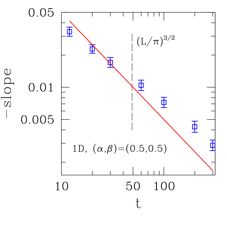
Figure 2: Linear chain with $N=41$ sites ($L=N+1$), $\alpha=\beta=1/2$. Double-logarithmic plot of (negative) initial slopes ($S$) of short-time density profiles against time $t$ (points). Continuous line is the mean-field prediction $S=1/(2t)$, see Eq. (50). The vertical dashed line indicates the approximate limit of validity of the short-time regime (see text).

Next we checked the late-time behavior, both for 1D systems and for nanotubes. Fig. 3 shows a fit of Eq. (21) to the ensemble-averaged density profile for a 1D system, starting from an empty lattice at $t=0$. While the quality of fit is good, with $\chi^{2}$ per degree of freedom ($\chi^{2}_{\rm dof}$) equal to $1.35$, one sees that small systematic deviations still remain near the left (injection) edge. Going over to later times in order to evince the suppression of such deviations would necessitate much narrower error bars (since one would be analyzing profiles much closer to the asymptotic regime), and consequently much longer simulations, than in our current setup.

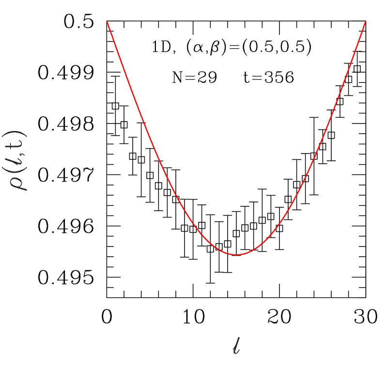
Figure 3: Linear chain with $N=29$ sites, $\alpha=\beta=1/2$. Plot of late-time density profile, starting with an empty lattice at $t=0$. Continuous line is the fit to a sine form, see Eq. (21) and text.

Nevertheless, we now show that it is possible to extract rather accurate estimates of the dynamic exponent $z$ from our data in present form, by once again referring to the ideas sketched in the last two paragraphs of Sec. II.1. Specifically we rewrite Eq. (21) as

$$\rho(\ell,t)=\frac{1}{2}-a^{\,\prime}(L)\sin\left(\frac{\pi\ell}{L}\right)\exp\left\{-c\,\frac{t}{L^{z}}\right\}\ ,$$ (51)

i.e., while assuming factorization of the $\ell$ and $t$ dependences, we allow $z$ to be a variable parameter. For fixed $L$ and a set of suitable $t$ values, fitting numerically-generated profiles to the sine dependence in Eq. (51) produces a sequence of estimates of

$$a^{\ast}(L,t)\equiv a^{\,\prime}(L)\,\exp\left\{-c\,\frac{t}{L^{z}}\right\}\ ;$$ (52)

the latter set is then fitted to

$$a^{\ast}(L,t)=a_{0}(L)\exp\{-c{\,{}^{\prime}}(L)\,t\}\ ,$$ (53)

with $a_{0}(L)$, $c{\,{}^{\prime}}(L)$ as fitting parameters. Finally, varying $L$ one fits the corresponding sequence of $c^{\,\prime}(L)$ to a power-law in $L$, thus extracting $z$.

We proceeded as just outlined for: (i) 1D systems, starting with an empty lattice; (ii) 1D systems, starting with a "sine-like" profile, i.e.,

$$n_{\ell}(0)=\begin{cases}{1\quad\ell\leq\frac{N}{4}\ {\rm or}\ \ell\geq\frac{3N}{4}}\cr{0\quad\frac{N}{4}<\ell<\frac{3N}{4}}\end{cases}\ ,$$ (54)

in order to check how sensitive the small late-time systematic deviations, referred to above, were to the choice of initial condition; (iii) nanotubes with $N_{w}=14$ elementary cells across and varying length $N_{r}$; and finally (iv) nanotubes with $N_{w}=N_{r}$ cells, i.e. aspect ratio equal to unity. In the latter two cases, sine-like initial profiles were used.

For (i)–(iii) we took $N=29$, $41$, $53$, and $69$ (corresponding, for nanotubes, to $N_{r}=7$, $10$, $13$, and $17$) and, for each of these, five $N$- (or $L$)-dependent values of $t$ in the late-time approach to steady state. We found that using a sine-like profile as initial condition does slightly improve the quality of profile fits to Eq.( 21). For example, in the corresponding case to that illustrated in Fig. 3, we found $\chi^{2}_{\rm dof}=0.91$, about a third less than for an empty-lattice start.

By following the fitting procedures delineated above our final results were  $z=1.51(1)$ in case (i), $z=1.54(1)$ in case (ii). The main diagram in Fig. 4 illustrates how well the numerically-evaluated coefficients $a^{\ast}(L,t)$ follow an exponential decay in time. That, as well as the smooth power-law fit of $c^{\,\prime}(L)$ against $L$ shown in the inset, gives strong support to the ansatz described in Eqs. (51)– (53).

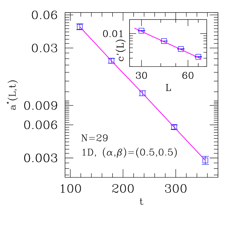
Figure 4: Main diagram: log-linear plot of $a^{\ast}(L,t)$ of Eq. (52) against $t$ for linear chain with $N=29$ sites. The continuous line connects numerically-obtained points. Initial condition: sine-like. Inset: double-logarithmic plot of $c^{\,\prime}(L)$ of Eq. (53) against $L\equiv N+1$. The continuous line is a fit of data to $c^{\,\prime}(L)\sim L^{-z}$, with $z=1.51$. Initial condition: empty lattice.

Analysis of case (iii) for the nanotube produced a less clear-cut picture concerning the final estimate of $z$. Although the exponential decay in time of the $a^{\ast}(L,t)$ still holds to excellent accuracy, resulting in the coefficients $c^{\,\prime}(L)$ listed under the heading $(a)\ N_{w}=14$ in Table 1, a single power-law fit of the latter against $L$ gives $z=1.76(2)$. By drawing on ideas for successively iterating sequences of finite-size approximants of quantities of interest bn , we produced a set of two-point fits of data for pairs $(L_{1},L_{2})=(30,42)$, $(42,54)$, and $(54,70)$. Plotting such set against $2/(L_{1}+L_{2})$, we arrived at the following extrapolated values for $2/(L_{1}+L_{2})\to 0$: $z=1.58(1)$ for a linear fit, $z=1.51(2)$ for a parabolic fit, see Fig. 5.

In case (iv) we took $N_{r}=N_{w}=8$, $12$, $16$, and $22$. The sequence of coefficients $c^{\,\prime}(L)$, obtained along the same lines already described, is given in Table 1, under $(b)$ Aspect Ratio$=1$. As shown in Fig. 5, by iterating two-point fits for pairs of successive lengths ones gets an increasing sequence of estimates of $z$ against increasing $L$. A straight-line fit gives an extrapolated $z=2.04(4)$. So this indicates that, while keeping $N_{w}>1$ fixed one gets essentially one-dimensional (critical) behavior, allowing for a constant aspect ratio of order unity one picks (asymptotically) the true two-dimensional dynamics. Furthermore, numerics indicate that the latter is characterized by the mean field exponent $z=2$.

Table 1: For nanotubes with $p=2q=1$, $(\alpha,\beta)=(1/2,1/2)$, late-time coefficients $c^{\,\prime}(L)$ of Eq. (53), obtained by the fitting procedure described in the text, for varying system lengths $L$. $(a)$: fixed width $N_{w}=14$ hexagons; $(b)$ aspect ratio $=1$.

$\ \ \ L$		$c^{\,\prime}(L)$
	$\ (a)\ N_{w}=14$
$\ \ \ 30$		$\,0.00859(12)$
$\ \ \ 42$		$0.00458(2)$
$\ \ \ 54$		$0.00291(3)$
$\ \ \ 70$		$0.00185(2)$
	$\ (b)\ \ {\rm Aspect\ Ratio}=1$
$\ \ \ 34$		$0.00670(2)$
$\ \ \ 50$		$0.00340(3)$
$\ \ \ 66$		$0.00203(1)$
$\ \ \ 90$		$0.00113(1)$

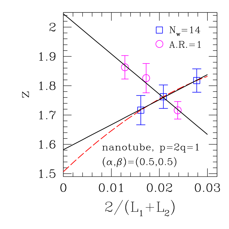
Figure 5: Nanotube with $p=2q=1$ at critical point $(\alpha,\beta)=(1/2,1/2)$. Points are estimates of dynamical exponent $z$ resulting from two-point fits of $c^{\,\prime}(L)$ in Table 1 for pairs of successive lengths $(L_{1},L_{2})$, against $2/(L_{1}+L_{2})$. Squares: fixed width $N_{w}=14$. Circles: fixed aspect ratio (A. R.)$=1$. Full lines: linear fits. Dashed line: parabolic fit [ for $N_{w}=14$ only ] (see text). Initial condition: sine-like in all cases.

Going back to the data for fixed $N_{w}$, for the nanotube with $p=2q=1$, $(\alpha,\beta)=(1/2,1/2)$ there appears to be a slow crossover towards $z=3/2$ behavior against increasing system size, which does not have a parallel in strictly 1D systems.

We have checked this scenario by investigating a steady-state quantity which is well-known to display signatures of anomalous scaling, namely the cumulants of the integrated current kvo10 ; dq12 . Denoting by $J$ the steady-state average current through a specified bond, say the one linking sites $\ell$ and $\ell+1$, and $J_{\ell\,\ell+1}(t^{\prime})$ its instantaneous value, the associated integrated charge is ${\widetilde{Q}}_{\ell\,\ell+1}(t)\equiv\int_{0}^{t}J_{\ell\,\ell+1}(t^{\prime})\,dt^{\prime}$. Usually one removes the linear term, and considers

$$Q(t)\equiv{\widetilde{Q}}(t)-Jt\ ,$$ (55)

so $\langle Q(t)\rangle\equiv 0$. For 1D TASEP at ($\alpha,\beta)=(1/2,1/2)$ the second-order cumulant $\langle\langle Q^{2}\rangle\rangle$ of the integrated current has been shown kvo10 ; dq12 to exhibit anomalous scaling, i.e., $\langle\langle Q^{2}(t)\rangle\rangle\sim t^{1/z}$ with $z=3/2$ along a time "window" of width determined by system size ("normal" scaling would correspond to $\langle\langle Q^{n}(t)\rangle\rangle\sim t$ for all $n$). In Fig. 6 we show data for both 1D systems, and for a nanotube with $N_{w}=12$, $N_{r}=10$ ($N=41$). The apparent behavior $\propto t^{0.57}$ exhibited for $200\lesssim t\lesssim 5\times 10^{4}$ by the latter is consistent with $\langle\langle Q^{2}(t)\rangle\rangle\sim t^{1/z}$, using the effective exponent $z=1.76(2)$ found from a global analysis of the $c^{\,\prime}(L)$ for fixed $N_{w}$ of Table 1.

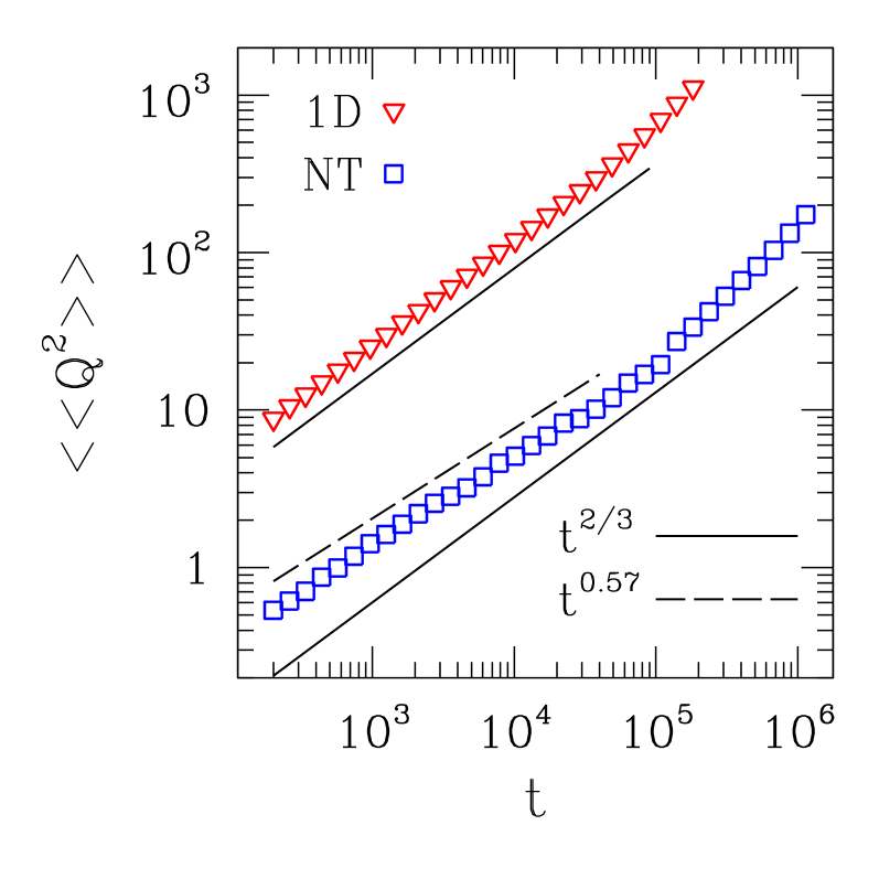
Figure 6: Points represent numerically-evaluated second cumulant $\langle\langle Q^{2}(t)\rangle\rangle$ of integrated steady-state current versus time $t$, for $(\alpha,\beta)=(1/2,1/2)$. 1D: linear chain, $N=600$ (adapted from Ref. dq12, ). NT: nanotube of width $N_{w}=12$ hexagons, $N=41$, with bond rates $p=2q=1$. Lines indicate power-law dependence with exponents as shown (see text).

Still for the nanotube, one can see behavior compatible with $\langle\langle Q^{2}(t)\rangle\rangle\sim t^{2/3}$ for $5\times 10^{4}\lesssim t\lesssim 2\times 10^{5}$, until it crosses over to "normal" scaling $\langle\langle Q^{2}(t)\rangle\rangle\sim t$ (of course the latter also takes place for 1D systems, see the corresponding data in Fig. 6). The narrowness of the $t^{2/3}$ "window" is most likely related to the relatively small (longitudinal) system size $N$ kvo10 ; dq12 .

So in the quasi-one dimensional limit for the $p=2q$ nanotube at criticality, the evidence provided both by dynamics (from the scaling of the $c^{\,\prime}(L)$ of Eq. (53) against $L$) and steady-state (from the scaling of $\langle\langle Q^{2}(t)\rangle\rangle$ against $t$) consistently points to an apparent $z\simeq 1.76$ for relatively short systems, and/or short times (the latter, after full onset of the steady-state regime), followed by a crossover towards $z=3/2$ in this case.

III.2 $p=2q$, $\alpha+\beta=1$

For $\alpha+\beta=1$, away from the critical point which was the subject of Sec. III.1, we took a point in the low current phase of 1D TASEP, namely $\alpha=0.3$, $\beta=0.7$.

Considering 1D systems, starting from an empty lattice, we adapted Eq. (25) for very late times such that only the $n=1$ term in that Equation still survives. In order to investigate density profiles in this regime we write:

$$\rho(\ell,t)=0.3-a(L,t)\,\sin\left(\frac{\pi\ell}{L}\right)\,e^{b\ell}\ ,$$ (56)

where $a(L,t)$ incorporates the exponential time dependence in Eq. (25), and the factor $b$ in Eq. (56) is predicted to be $b=\lambda=0.4$. In Fig. 7, for 1D TASEP with $N=29$, curve (I) [ full red line ] shows the best fit of Eq. (56) to the simulational results given there, corresponding to $a=35(4)\times 10^{-5}$, $b=0.144(6)$, with $\chi^{2}_{\rm dof}=1.8$.

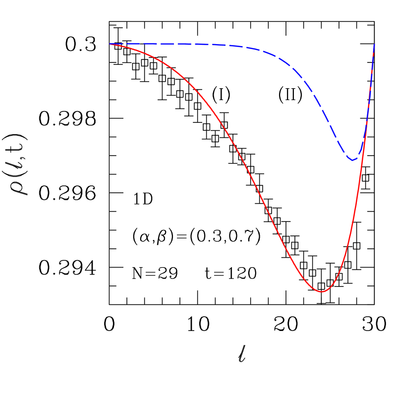
Figure 7: Linear chain with $N=29$ sites, $\alpha=0.3$, $\beta=0.7$, $p=2q=1$. Plot of late-time density profile, starting with an empty lattice at $t=0$. Curve (I) is a fit to a sine plus exponential form, with $a$ and $b$ of Eq. (56) as adjustable parameters; curve (II) is the prediction from Eq. (25), adjusted to the empty-lattice initial condition, and using only $n=1$; see text.

Curve (II) [ dashed blue line] is the prediction of Eq. (25) with $\lambda=0.4$, with the $\{a_{\zeta_{n}}\}$ adjusted to an empty-lattice initial condition and using only the $n=1$ term.

Although their overall shape is similar, curves (I) and (II) significantly differ in (a) the depth and, to a lesser extent, location, of the minimum on the right-hand side, and (b) the nearly-horizontal segment stretching almost midway through the system, exhibited by curve (II), which has no counterpart in curve (I). While making $t\approx 110$ in Eq. (25), instead of "simulation time" $t=120$ reproduces the minimum value shown by numerical data (its location, however, remaining unchanged within one lattice spacing), point (b) is a permanent feature of the theoretical prediction which reflects the large value of $\lambda=0.4$ in the profile’s exponential $\ell-$dependence in Eq. (25).

The discrepancy between the optimally adjusted value of the exponential prefactor $b$ of Eq. (56), on the one hand, and the theoretical prediction of $\lambda=1-2\alpha$ on the other, is undoubtedly significant. This indicates that, although simple adaptations enable it to give an accurate description of the critical systems of Sec. III.1, the mean-field theory given above does not quantitatively account for the effects of a characteristic inverse length $\lambda\neq 0$ in a similarly straightforward way. We have found unpub that a formulation including the effects of stochastic domain-wall hopping ksks98 ; ps99 ; ds00 on early- and late-time profiles can account for most of the quantitative mismatches between mean-field theory predictions and simulational results for non-critical cases.

However, in the present work we limit ourselves to analysing the extent to which the mean field theory of Sec. II can provide useful clues to the actual behavior of numerically-generated samples. Thus, here we attempt a procedure similar to that described in Sec. III.1 for extraction of the dynamical exponent.

In addition to 1D systems, and similarly to Sec. III.1, we considered nanotubes both (1) with $N_{w}=14$ elementary cells across and varying length $N_{r}$, and (2) with unit aspect ratio ($N_{w}=N_{r}$ cells). The time dependences predicted respectively in Eqs. (21), related to the critical ("gapless") phase and (25) for the "massive" or "gapped" phase, differ in that the decay rate in the latter has an $L-$independent term, the gap [ equal to $\lambda^{2}/2\,$], related to the characteristic inverse length $\lambda$.

In an attempt to give similar relative importance, when compared to the gap contribution, to the finite-size dependence to the exponential time decay we used $N_{r}=2$, $3$, $4$, and $5$, corresponding to $N=9$, $13$, $17$, and $21$ sites.

Again, we generated each $a(L,t)$ from adjusting late-time profiles to Eq. (56), by allowing both $a$ and $b$ there to vary. We saw that the fitted value of $b$ generally stayed between $0.15$ and $0.28$.

We then fitted sequences of varying-$L$ data for $a(L,t)$ to the $n=1$ term of Eq. (25), i.e., $a(L,t)=a_{0}\,\exp(-c_{0}(L)\,t)$, with $c_{0}(L)=c+d/L^{z}$.

Allowing $z$ to vary freely gave a large amount of scatter ($0.5\lesssim z\lesssim 3.5$) among fits of four-$L$ data for the three different geometries [ chains, and nanotubes with either $N_{w}=14$ or unit aspect ratio ]. We then recalled that, for 1D systems in the low-current phase $\alpha<1/2$ or $\beta<1/2$ (except on the coexistence line $\alpha=\beta<1/2$) the effective exponent governing the approach to steady state is $z^{\prime}=1$ dqrbs08 . This is in contrast to the result from a rigorous Bethe ansatz calculation ess05 , namely $z=0$, and can be explained by a mean-field continuum formulation related to kinematic-wave propagation dqrbs08 . Thus we plotted our data for $c_{0}(L)$ against $1/L$, i.e. keeping $z^{\prime}=1$ fixed. The results are shown in Fig. 8.

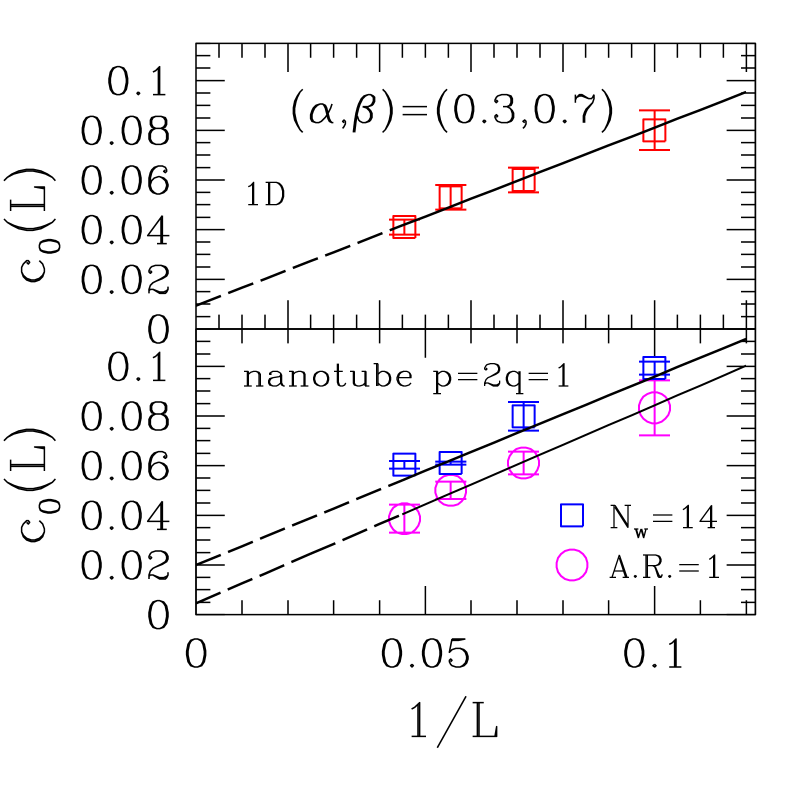
Figure 8: For systems with $\alpha=0.3$, $\beta=0.7$, plots of $c_{0}(L)$ against $1/L$, with $c_{0}(L)$ defined via $a(L,t)=a_{0}\,\exp(-c_{0}(L)\,t)$, the $a(L,t)$ being given by fitting Eq. (56) to late-time profiles. Upper diagram: 1D systems. Lower diagram: nanotubes with $p=2q=1$; squares: fixed width $N_{w}=14$; circles: fixed aspect ratio (A. R.)=1.

It is seen that the numerical data for the sequences of $c_{0}(L)$ fall reasonably well onto a straight line consistent with $z=1$, for all three geometries considered. From the vertical axis intercepts one gets respectively $c=0.009(5)$ (1D), $c=0.02(1)$ (nanotube with $N_{w}=14$), and $c=0.0046(44)$ (nanotube with unit aspect ratio). These are all definitely much lower than the mean-field prediction $\lambda^{2}/2=0.08$. It seems plausible from these data that the gap will vanish for very large nanotubes with finite aspect ratio (remaining finite in the quasi- and strictly 1D cases). However, the relatively poor quality of the fits [$\,\chi^{2}_{\rm dof}=0.36$, $10$ and $0.14$, listed for each geometry in the same order as the $c$ values ] indicates that a statement of this sort would have to be tested more extensively.

III.3 $p\neq 2q$

Initially we investigate the nanotube with $p=q=1$ at $\alpha_{c}=2(\sqrt{2}-1)$, $\beta_{c}=2-\sqrt{2}$. These rates satisfy the conditions specified in Eqs. (26)– (28), for which the Mobius mapping predicts uniform steady state densities on each sublattice, though in general they remain distinct; namely, in this case they are $x^{\ast}=2-\sqrt{2}$, $y^{\ast}=\sqrt{2}-1$.

For comparison, we consider also the chain with alternating bond rates $p$, $2q$ with $p=q=1/2$. The mean-field Mobius mapping for this case coincides with that for the $p=q=1$ nanotube, provided the injection/ejection rates are suitably renormalised, i.e. $\alpha=\sqrt{2}-1$, $\beta=1-\sqrt{2}/2$. The respective steady state sublattice densities are then predicted to coincide, though of course the rate of approach to steady state on the alternate-bond chain is half that for the nanotube.

We took $N_{w}=14$, $N_{r}=10$ for the nanotube, and $N=41$ sites for the chain so both have the same number of sites along the flow direction. For the remainder of this Section, in both cases we always started with an empty lattice.

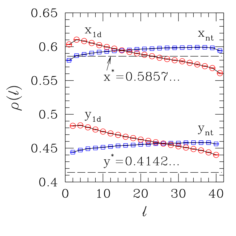
Figure 9: Steady state sublattice densities against position along flow direction for nanotube $p=q=1$ (squares: $x_{nt}$, $y_{nt}$) at $\alpha=2(\sqrt{2}-1)$, $\beta=2-\sqrt{2}$, and for chain with alternating bond rates $p$, $2q$ with $p=q=1/2$ (circles: $x_{1d}$, $y_{1d}$) at $\alpha=\sqrt{2}-1$, $\beta=1-\sqrt{2}/2$ (see text). Horizontal dashed lines show mean field predictions applying for both cases: $x^{\ast}=2-\sqrt{2}$, $y^{\ast}=\sqrt{2}-1$.

Fig. 9 shows that the mean field prediction of flat sublattice density profiles in steady state is not fulfilled in numerical simulations. Also, the sublattice profiles for the nanotube and the alternating-bond chain do not coincide, at variance with the fact that they share the same description via mean-field mapping. However, the mean field mapping predicts the steady-state sublattice densities to within at most $4\%$ (for $x^{\ast}$) or $16\%$ (for $y^{\ast}$) of numerical results. Since the predicted densities are themselves separated by just over $40\%$, one can unequivocally ascribe each predicted sublattice profile to the correct numerically-generated subset of results.

We defer further discussion of such discrepancies, and others which also pertain to steady-state aspects, to Sec. III.4 below. For the moment we investigate, for nanotubes with $p=q=1$, the very late time behavior of the density profiles. Allowing for the observed non-uniformity of their limiting steady-state shapes, Eqs. (47) and (48) for a system at criticality should translate into:

$$x_{\ell}(t)=x_{\ell}^{\ast}+G^{\prime}\sin\frac{\pi\ell}{L}\,e^{-\lambda_{-}(\pi/L)\,t}$$ (57)

$$y_{\ell}(t)=y_{\ell}^{\ast}+H^{\prime}\sin\frac{\pi\ell}{L}\,e^{-\lambda_{-}(\pi/L)\,t}$$ (58)

where now the position-dependent $x_{\ell}^{\ast}$, $y_{\ell}^{\ast}$ are to be numerically obtained from steady-state simulation data.

Results for the difference profiles, $\delta x_{\ell}(t)\equiv x_{\ell}(t)-x_{\ell}^{\ast}$ and the similarly defined $\delta y_{\ell}(t)$, for the nanotube with $p=q=1$, $\alpha=2(\sqrt{2}-1)$, $\beta=2-\sqrt{2}$ are exhibited in Fig. 10. Late-time data were taken at $t=500$ (for comparison, the corresponding steady-state densities shown in Fig. 9 were taken at $t=2500$).

It is seen that the spatial dependence of $\delta x_{\ell}(t)$ and $\delta y_{\ell}(t)$ is indeed very close to that anticipated in Eqs. (57), (58), although the numerical results show a slight skew. The fit to a sine form shown as a dashed line in Fig. 10 corresponds to $\chi^{2}_{\rm dof}=49$, which is unsatisfactory. We then allowed for a nonzero gap, by returning to the more general expressions Eqs. (37) and (38). Fitting to the $n=1$ term of Eq. (37), i.e.,

$$\delta x_{\ell}(t)=-a(t)\,e^{\phi\ell}\,\sin\left(\frac{\pi\ell}{L}\right)\ ,$$ (59)

we found the full-line curve depicted in Fig. 10, with $\phi=-0.022(1)$, $\chi^{2}_{\rm dof}=3.2$. The small, but definitely non-zero, estimate of $\phi$ is in line with the steady-state results shown in Fig. 9 in that both indicate the approximate, rather than exact, character of the mean-field description for $p\neq 2q$.

Furthermore, the difference profiles are almost entirely sublattice-independent, a feature which is not obviously forthcoming from the theory of Sec. II.2. It can be shown (see Appendix A) that this results from the existence of two distinct relaxation rates: one which is very fast, size-independent [ which brings the sublattice profiles to shapes rather close to their steady-state ones ] and a slower one, with characteristic times of the usual $L^{z}$ form. In the (not very short)-time regime for which the latter applies the sublattice distinction disappears for difference profiles, and the dynamics can be described in an effective continuum approximation through linear equations resulting from a Cole-Hopf transformation. For example, difference profiles taken at $t=250$ for the system considered in Fig. 10 already exhibit a degree of sublattice-independence very similar to that shown in the Figure. Using Eqs. (57), (58) for simplicity, defining $G^{\prime\prime}(t)\equiv G^{\prime}\,e^{-\lambda_{-}(\pi/L)t}$ one finds by fitting numerical data $G^{\prime\prime}(250)/G^{\prime\prime}(500)\approx 4.4$, which corresponds to $\lambda_{-}(\pi/L)\approx 6\times 10^{-3}$. Direct evaluation via the theoretical prediction Eq. (49), using the mean field values for $x^{\ast}$, $y^{\ast}$, $r$ from Eqs. (28) and (32) gives $\lambda_{-}(\pi/L)=1.0\times 10^{-3}$.

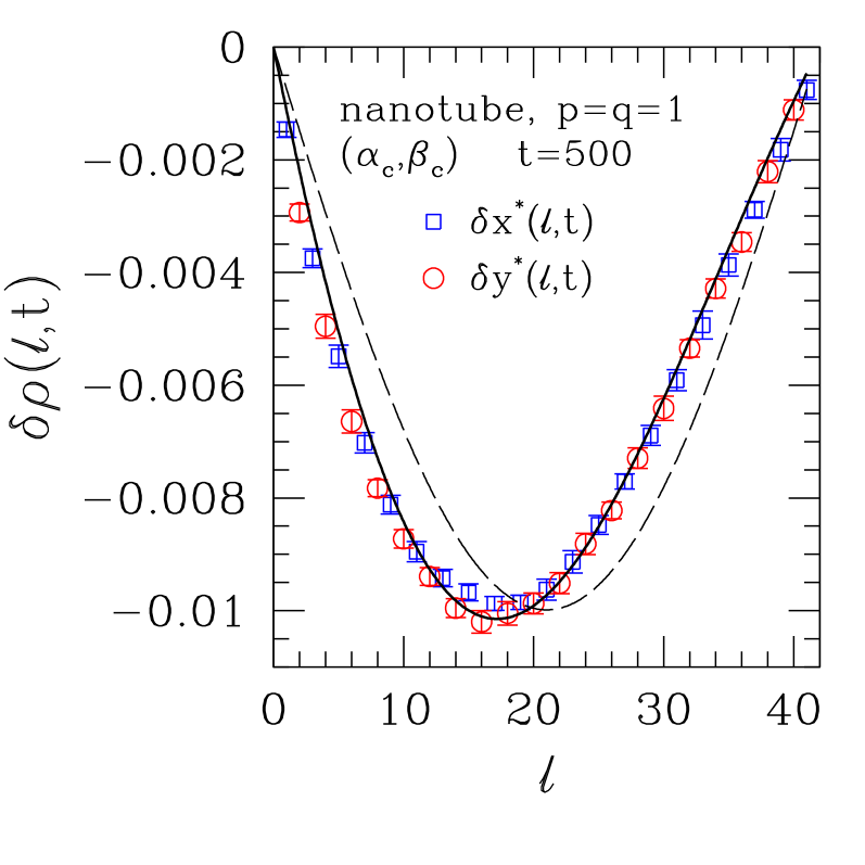
Figure 10: Late-time difference profiles, $\delta x_{\ell}(t)\equiv x_{\ell}(t)-x_{\ell}^{\ast}$, and similarly for $\delta y_{\ell}(t)$, against position along flow direction for nanotube $p=q=1$ at $\alpha_{c}=2(\sqrt{2}-1)$, $\beta_{c}=2-\sqrt{2}$, for $t=500$. The dashed line is the fit of $\delta x_{\ell}(t)$ to a sine form, see Eqs. (57), (58). The full line is a fit of $\delta x_{\ell}(t)$ to a sine-plus-exponential form, see Eq. (59) and text.

Turning now to non-critical systems, proceeding along the lines followed above one can again adapt Eqs. (37), (38) to make allowance for the position dependence of steady state profiles, for systems away from criticality but with $\alpha$ and $\beta$ obeying Eq. (26).

For $\alpha=0.4$, $\beta=0.8$ the numerically-obtained steady state profiles turned out to be nearly flat down to $3-4$ parts in $1000$, with $x_{\ell}\approx 0.324$, $y_{\ell}\approx 0.209$, except very near the system’s ends. These values are rather close to the mean field ones predicted via Eq. (28), namely $x_{\ell}=1/3$, $y_{\ell}=1/5$ . The late-time difference profiles obtained in the way described above, at $t=100$, are displayed in Fig. 11. Fitting to Eq. (59) gives a fairly good account of the behavior of $\delta x_{\ell}(t)$ against $\ell$; also, the sublattice independence of difference profiles is obeyed to a good extent, though some slight discrepancies remain near the ejection end. From Eqs. (28), (37)–(41), theory predicts that the coefficient $\phi$ in the position dependence of late-time density profiles should be $\phi=(\ln 8)/2=1.04\dots$, and that for the time dependence the slowest decay rate should be $\lambda_{1}^{T}=0.166\dots$.

The fitting curve shown in Fig. 11 corresponds to $\phi=0.34(1)$. A measure of self-consistency of the latter can be gained by pointing out that, if $\phi L\gtrsim 5-6$ the minimum of Eq. (59) is located at $\ell\approx L-(1/\phi)$. Visual inspection of Fig. 11 confirms that numerical data indeed behave in this way. On the other hand, the mismatch between predicted and observed values of $\phi$ is a rather extreme illustration of the limitations of mean field mapping predictions for $p\neq 2q$, already evident e.g. in the density profiles of Fig. 9.

We checked the theoretical prediction for $\lambda_{1}$ by comparing difference profiles at $t=80$ with those for $t=100$. Referring to Eq. (59), one gets $a(100)/a(80)=0.08\pm 0.05$, broadly compatible with $e^{-20\,\lambda_{1}^{T}}=0.03615\dots$.

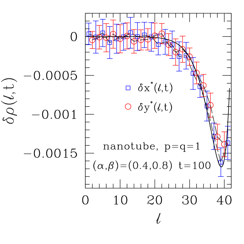
Figure 11: Late-time difference profiles, $\delta x_{\ell}(t)\equiv x_{\ell}(t)-x_{\ell}^{\ast}$, and similarly for $\delta y_{\ell}(t)$, against position along flow direction for nanotube $p=q=1$ at $\alpha=0.4$, $\beta=0.8$, for $t=100$. The full line is the fit of $\delta x_{\ell}(t)$ to a sine plus exponential form, using only the $n=1$ term of Eq. (37) [ in an adapted form to allow for the position dependence of steady state profiles, see text ].

III.4 Factorization in steady state

It was seen in Sec. III.3 that numerical results for steady state density profiles on nanotubes and alternating-bond chains with $p\neq 2q$ are at variance with the predictions of mean field Mobius mapping. Mismatches of similar order have been found between mean-field results and numerical work regarding steady-state currents in graphene-like structures with $p\neq 2q$ hex13 .

In the following, we expand on comments made in Ref. hex13, , regarding the issue of factorization in steady state.

It is known for the strictly one-dimensional TASEP that, along $\alpha+\beta=1$ the correlations vanish, i.e., the probabilities for occupation variables on different sites factorize derr93 . As a consequence of this, along that line the mean field mapping produces exact results. For nanotubes one can then check for factorization (or its absence), in order to test the extent to which the predictions given via Mobius mappings are accurate.

A direct test can be implemented by considering the (connected) correlation function,

$$C_{ij}\equiv\langle J_{ij}\rangle-p_{ij}\,\langle\tau_{i}\rangle\,\left(1-\langle\tau_{j}\rangle\right)\ ,$$ (60)

where $\langle J_{ij}\rangle$ is the average current across a chosen bond $ij$ with rate $p_{ij}$, connecting sites $i$, $j$ with respective mean occupations $\langle\tau_{i}\rangle$, $\langle\tau_{j}\rangle$. Factorization then corresponds to $C_{ij}\equiv 0$ for all bonds $ij$.

We have found that for the nanotube with $p=1$, $q=1/2$ $C_{ij}$ vanishes to the accuracy of simulation (typically $1$ part in $10^{5}$) on (and only on) the line $\alpha+\beta=1$, the same as in the strictly one-dimensional case. This is a non-trivial higher-dimensional generalization of a well known result for the linear chain. On the other hand, with $p=1=q=1$, we followed the predicted factorization line, Eq. (26), and found that in simulations of similar accuracy, the factorization is no better than $1$ part in $10^{2}$. This is illustrated in Fig. 12, where data taken at the respective predicted critical points, namely $\alpha=\beta=1/2$ [$\,p=2q=1\,$] and $\alpha=2(\sqrt{2}-1)$, $\beta=2-\sqrt{2}$ [$\,p=q=1\,$] are shown. For $p=q=1$, data are shown also for $(\alpha,\beta)=(0.4,0.8)$, i.e., further along the predicted factorization line Eq. (26).

Still with $p=q=1$ we thoroughly scanned the $(\alpha,\beta)$ parameter space, and found no evidence either of uniform sublattice profiles or of vanishing of $C_{ij}$.

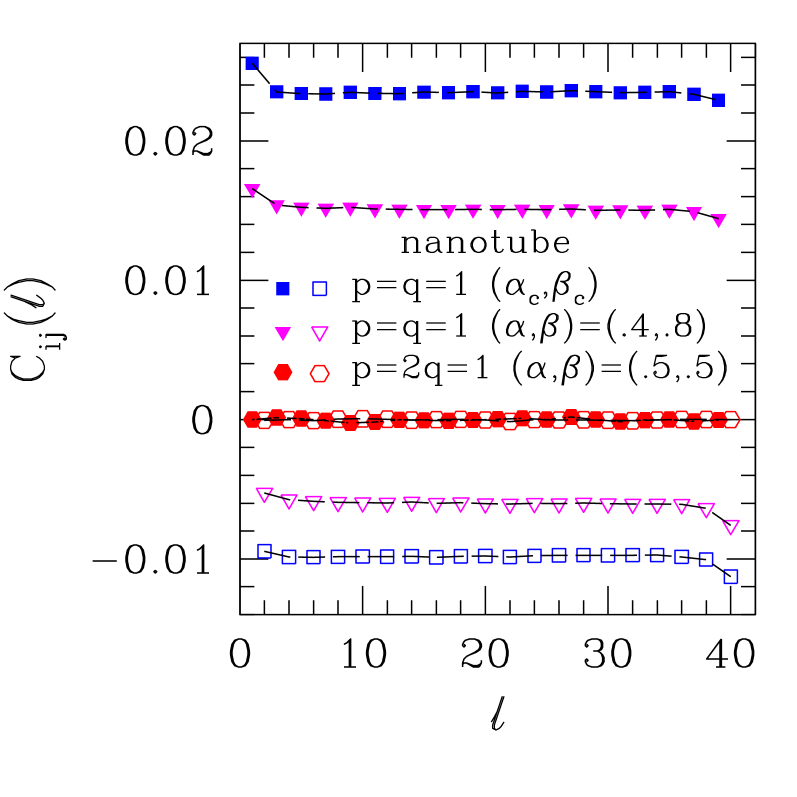
Figure 12: Nanotube with $N_{w}=14$, $N_{r}=10$: $C_{ij}$ of eq. (60), averaged over transverse coordinate, against position along flow direction. Full symbols: $x-$ sublattice. Empty symbols: $y-$ sublattice. For $p=q=1$, $(\alpha_{c},\beta_{c})=(2(\sqrt{2}-1),2-\sqrt{2})$.

IV Discussion and Conclusions

We have presented a mean-field theory for the dynamics of driven flow with exclusion in graphene-like structures, and numerically checked its predictions.

For the special combination of bond rates $p=2q$ in the nanotube geometry, Eqs. (2)–(5) show that the sublattice distinction goes away in mean field. So a continuum picture can apply, giving Eq. (11) for which a time-dependent solution is found by using the Cole-Hopf transformation.

For the special boundary rates $\alpha=\beta=1/2$ which corresponds to criticality in the 1D chain with uniform rates, predictions for the early– and late-time behavior of density profiles are made respectively in Eqs. (22) and (21). These are borne out by numerics to very good accuracy, see Figs. 2 and 3. We focused on late-time behavior, for both 1D and nanotube geometries, and showed that by systematically analyzing the results of density profile fits to Eq. (21) it was possible [ see Eqs. (51)– (53) ] to extract rather accurate estimates of the dynamic exponent $z$. For strictly 1D systems, we find $z=1.51(1)$, in excellent agreement with the anomalous value $z=3/2$ which is known derr98 ; sch00 ; rbs01 to apply in that case. For nanotubes, we found strong indications (see Fig. 5) that the limiting behavior for very long length depends on whether one considers (quasi-1D) systems of fixed width, or square-like ones with constant aspect ratio; while the former exhibit $z$ again close to $3/2$, the latter are characterized by $z$ consistent with the mean-field value of $2$ (within error bars). In the standard language of critical phenomena, this would mean that the upper critical dimensionality for TASEP dynamics is certainly $D_{c}\leq 2$.

On the factorization line $\alpha+\beta=1$ where steady-state profiles are uniform both for uniform-rate chains and nanotubes with $p=2q$ hex13 , we took $\alpha=0.3$, away from criticality. The main distinguishing feature here, relative to the critical case, is the opening of a gap of amplitude $\lambda^{2}/2=(1-2\alpha)^{2}/2$, associated with the characteristic length $\lambda^{-1}$. The predicted effects of this on late-time profile shapes are spelt out in Eq. (25), which is qualitatively supported by numerical data (see Fig. 7).

However, the quantitative effects, on the density profiles, of having $\lambda\neq 0$ are not accurately described by the present mean-field theory. Partly because of this, attempts to extract the dynamical exponent $z$, by procedures similar to those followed in the gapless case, met with the difficulties described in Sec. III.2.

We then resorted to an overall consistency check, based on keeping fixed the effective exponent value $z^{\prime}=1$ which holds for the low-current phase in 1D systems dqrbs08 . The resulting fits of numerical estimates of the coefficients appearing in the exponential time decay factor of Eq. (25), shown in Fig. 8, produce a reasonably self-consistent picture.

For nanotubes with $p\neq 2q$ (and chains with alternating bonds), Fig. 9 illustrates that predictions for steady state profiles from mean field mapping are not as accurate as for $p=2q$, or for uniform chains. In particular, numerically-generated profiles display a distinctive degree of nonuniformity along the predicted factorization line.

Since dynamics concerns the evolution from initial to steady state, rather than the detailed (time-independent) properties of the latter, we adapted our original formulation to allow for the observed non-uniformity of the sublattice-dependent limiting profile shapes, see Eqs. (57), (58) for critical systems, and Eq. (59) for the off-critical case. We found that for late times the difference profiles thus defined behave in a very close way to that predicted by the theory of Sec. II.2, see respectively Figs. 10 and 11.

This latter remark deserves to be qualified, inasmuch as it refers strictly to the functional forms displayed in Eqs. (57), (58), or Eq.( 59) [ respectively sine, or sine plus exponential ] rather than to numerical values of the associated parameters [ respectively $G^{\prime}$, $H^{\prime}$, or $a(t)$, $\phi\,$] which we estimate via best-fitting procedures. Although this is not as stringent a test of mean field theory as would be the case if the theory-predicted parameter values were used, working this way allows one to separate possible shortcomings of the mean field approximation in functional forms versus those in parameters. Furthermore, one can have a quantitative estimate (through $\chi^{2}$ values) of discrepancies in mean field functional forms, rather than the qualitative impressions from the comparisons with full predictions coming from theory; one can also get quantitative estimates of parameters affected by fluctuation effects absent from mean field theory, with the hope that modest generalizations (like domain wall theory) might more accurately provide such parameters.

An additional feature of the late-time difference profiles is that they are almost entirely sublattice-independent. This property has been shown (see Appendix A) to result from the coexistence of two distinct relaxation rates: a very fast, size-independent one, and a slower one with characteristic times of the usual $L^{z}$ form. The latter applies, within an effective continuum picture, to the Goldstone modes resulting from particle number conservation. If one accepts that an accurate description of TASEP via mean field mapping goes together with full applicability of a continuum approximation, this would then explain why the late-time density differences generally fall in line with mean-field, continuum-like, predictions.

Detailed comparison of theoretical predictions from Sec. II.2 to numerical results beyond overall profile shapes turns out to not be as accurate as for $p=2q$. For the system considered in Fig. 10 theory gives for the exponential time-decay coefficient of Eq. (49) $\lambda_{-}(\pi/L)=1\times 10^{-3}$, while adjusting to numerical data gives $\lambda_{-}(\pi/L)\approx 6\times 10^{-3}$. Similarly, for the non-critical system corresponding to Fig. 11, using the theoretical prediction for $\lambda_{1}$ of Eqs. (37), (38) would give a ratio of difference-profile coefficients at $t=100$ and $t=80$ equal to $0.03615\dots$, while this same ratio is estimated from numerical data as $0.08\pm 0.05$.

Finally, in Sec. III.4 we showed that a direct test of factorization of correlation functions in steady state produces a clear correspondence between uniformity of observed steady state profiles, on the one hand, and numerical evidence of vanishing of correlations, on the other.

Appendix A Fast transient equalization of sublattices

For our purposes here, it is convenient to adopt the following notation: sites on the $x-$ sublattice have even site label, with mean occupation $x_{2\ell}$; for the $y-$ sublattice, with odd labels one has the mean occupation $y_{2\ell+1}$. Bond rates are $p$ and $p^{\prime}\equiv 2q$.

Thus the mean field defining equations for currents and occupations, and their evolution, Eqs. (2)–(5), become

$$J_{2\ell\,2\ell+1}=p\,x_{2\ell}\,(1-y_{2\ell+1})\ \ \,$$ (61)

$$K_{2\ell-1\,2\ell}=p^{\prime}\,y_{2\ell-1}\,(1-x_{2\ell})\ .$$ (62)

$${\dot{x}}_{2\ell}=K_{2\ell-1\,2\ell}-J_{2\ell\,2\ell+1}\ \ \,$$ (63)

$${\dot{y}}_{2\ell+1}=J_{2\ell\,2\ell+1}-K_{2\ell+1\,2\ell+2}\ .$$ (64)

Eqs. (63) and (64) give:

$$\frac{\partial}{\partial t}\,\left(x_{2\ell}+y_{2\ell+1}\right)=K_{2\ell-1\,2\ell}-K_{2\ell+1\,2\ell+2}\ .$$ (65)

When a continuum picture applies, the right-hand side of Eq. (65) becomes like a space derivative of $K$ and is then small, so $x_{2\ell}+y_{2\ell+1}$ becomes a slow variable; similarly for $y_{2\ell-1}+x_{2\ell}$.

On the other hand, any linear combination $a\,x_{2\ell}+b\,y_{2\ell+1}$ with $a\neq b$ decays rapidly towards zero. This implies that the rapid decay is towards "adiabatic" values of $x_{2\ell}$, $y_{2\ell+1}$ such that all $K_{2\ell-1\,2\ell}-J_{2\ell\,2\ell+1}$ and $J_{2\ell\,2\ell+1}-K_{2\ell+1\,2\ell+2}$ are zero. That is,

$$K_{2\ell-1\,2\ell}=J_{2\ell\,2\ell+1}=J_{2\ell\,2\ell+1}=K_{2\ell+1\,2\ell+2}=\cdots=C(t)\ .$$ (66)

The function $C(t)$ is the adiabatically evolving "conserved current" related to the particle conservation represented by the set of equations Eq. (65) for all $\ell$. Those equations determine the adiabatic evolution of the conserved densities.

After the very fast transients have died out the profiles on the two sublattices still differ from their steady-state values $\bar{x}_{2\ell}$, $\bar{y}_{2\ell+1}$ by amounts $\delta x_{2\ell}(t)$, $\delta y_{2\ell+1}(t)$; as shown in the following, such differences are essentially the same for either sublattice, as their approach to zero is governed by a single continuum-like evolution equation.

The fast time scales for the evolution of $a\,x_{2\ell}+b\,y_{2\ell+1}$ with $a\neq b$, coming from equations without nearly cancelling currents, and so without conserved or spatial derivative aspects, have rates set just by $p$ and $p^{\prime}$, and not by wave vectors or system size $L$. So they are of order one, rather than a power of $L$ or wavelength.

In the subsequent evolution (after the initial transient regime) (i) we can interpolate the density variables between the sites of their sublattice, making very little error; and (ii) use the resulting "continuumization" of sites to find the conserved current differences in terms of spatial derivatives: e.g., $\widetilde{y}_{2\ell}$ is the interpolation of the odd sublattice variables $y_{2\ell-1}$, $y_{2\ell+1}$; similarly for $\widetilde{x}_{2\ell+1}$. So,

$$K_{2\ell-1\,2\ell}-K_{2\ell+1\,2\ell+2}=\qquad\qquad$$

$$=p^{\prime}\,\left[\,y_{2\ell-1}(1-x_{2\ell})-y_{2\ell+1}(1-x_{2\ell+2})\right]\approx\qquad\qquad$$

$$\approx p^{\prime}\,\left(-2\frac{\partial}{\partial\ell}\right)\,\left[\,\widetilde{y}_{2\ell}(1-\widetilde{x}_{2\ell+1})\right]\ ,\qquad\qquad$$ (67)

and similarly for differences of adjacent $J^{\prime}$s.

Combining Eqs. (65) and (67) [ and their counterparts for $y_{2\ell-1}+x_{2\ell}$ and $J_{2\ell-2\,2\ell-1}-J_{2\ell\,2\ell+1}$, respectively ], omitting the subscripts and tilde signs, redefining $\ell$ as an "average" coordinate shared by a pair of adjacent $x-$ and $y-$ subllattice sites, and defining $\rho(\ell)=\frac{1}{2}(x_{\ell}+y_{\ell})$, one gets:

$$\frac{\partial\rho}{\partial t}=-\left(\frac{p+p^{\prime}}{2}\right)\,\frac{\partial}{\partial\ell}\left[\rho(1-\rho)-\frac{1}{2}\frac{\partial\rho}{\partial\ell}\right]\ .$$ (68)

This is now the form which the Cole-Hopf transformation linearizes.

References

- (1) R. B. Stinchcombe, S. L. A. de Queiroz, M. A. G. Cunha, and Belita Koiller, Phys. Rev. E88, 042133 (2013).
- (2) B. Derrida, Phys. Rep. 301, 65 (1998).
- (3) G. M. Schütz, in Phase Transitions and Critical Phenomena, edited by C. Domb and J. L. Lebowitz (Academic, New York, 2000), Vol. 19.
- (4) B. Derrida, E. Domany, and D. Mukamel, J. Stat. Phys. 69, 667 (1992).
- (5) B. Derrida, M. Evans, V. Hakim, and V. Pasquier, J. Phys. A 26, 1493 (1993).
- (6) R. B. Stinchcombe, Adv. Phys. 50, 431 (2001).
- (7) R. A. Blythe and M. R. Evans, J. Phys. A 40, R333 (2007).
- (8) T. Chou, K. Mallick, and R. K. P. Zia, Rep. Prog. Phys. 74, 116601 (2011).
- (9) B. Schmittmann and R. K. P. Zia, in Phase Transitions and Critical Phenomena, edited by C. Domb and J. L. Lebowitz (Academic, New York, 1995), Vol. 17.
- (10) R. Bundschuh, Phys. Rev. E65, 031911 (2002).
- (11) T. Karzig and F. von Oppen, Phys. Rev. B81, 045317 (2010).
- (12) N. Rajewsky, L. Santen, A. Schadschneider, and M. Schreckenberg, J. Stat. Phys. 92, 151 (1998).
- (13) S. L. A. de Queiroz and R. B. Stinchcombe, Phys. Rev. E78, 031106 (2008).
- (14) J-C. Charlier, X. Blase, and S. Roche, Rev. Mod. Phys. 79, 677 (2007); A. H. Castro Neto, F. Guinea, N. M. R. Peres, K. S. Novoselov, and A. K. Geim, ibid. 81, 109 (2009).
- (15) E. Hopf, Commun. Pure Appl. Math. 3, 201 (1950).
- (16) J. D. Cole, Q. Appl. Math. 9, 225 (1951).
- (17) M. P. Nightingale and H. W. J. Blöte, J. Phys. A 15, L33 (1982); H. W. J. Blöte and M. P. Nightingale, Physica A 112, 405 (1982); ibid, 134, 274 (1985).
- (18) S. L. A. de Queiroz, Phys. Rev. E86, 041127 (2012).
- (19) R. B. Stinchcombe and S. L. A. de Queiroz, unpublished.
- (20) A. B. Kolomeisky, G. M. Schütz, E. B. Kolomeisky, and J. P. Straley, J. Phys. A 31, 6911 (1998).
- (21) V. Popkov and G. M. Schütz, Europhys. Lett. 48, 257 (1999).
- (22) M. Dudzinsky and G. M. Schütz, J. Phys. A 33, 8351 (2000).
- (23) J. de Gier and F. H. L. Essler, Phys. Rev. Lett. 95, 240601 (2005); J. Stat. Mech.: Theory Exp. (2006) P12011.