Localising fast radio bursts and other transients using interferometric arrays

A new population of sources emitting fast and bright transient radio bursts, called FRBs, has recently been identified. The observed large dispersion measure values of FRBs suggests an extragalactic origin and an accurate determination of their positions and distances will provide an unique opportunity to study the magneto-ionic properties of the intergalactic medium. So far, FRBs have all been found using large dishes equipped with multi-pixel arrays. While large single dishes are well-suited for the discovery of transient sources they are poor at providing accurate localisations. A two-dimensional snapshot image of the sky, made with a correlation interferometer array, can provide an accurate localisation of many compact radio sources simultaneously. However, the required time resolution to detect FRBs and a desire to detect them in real time, makes this currently impractical. In a beamforming approach to interferometry, where many narrow tied-array beams (TABs) are produced, the advantages of single dishes and interferometers can be combined. We present a proof-of-concept analysis of a new non-imaging method that utilises the additional spectral and comparative spatial information obtained from multiple overlapping TABs to estimate a transient source location with up to arcsecond accuracy in almost real time. We show that this method can work for a variety of interferometric configurations, including for LOFAR and MeerKAT, and that the estimated angular position may be sufficient to identify a host galaxy, or other related object, without reference to other simultaneous or follow-up observations. With this method, many transient sources can be localised to small fractions of a half-power-beamwidth (HPBW) of a TAB, in the case of MeerKAT, sufficient to localise a source to arcsecond accuracy. In cases where the position is less accurately determined we can still significantly reduce the area that need be searched for associated emission at other wavelengths and potential host galaxies.

1 Introduction

In the past few years, a possible new population of sources emitting fast and bright transient radio bursts has been discovered. In August 2001 an isolated pulse of radio emission was recorded but was only discovered during the analysis of the archival survey data of the Magellanic clouds (Manchester et al., 2006). The discovery was published in 2007 (Lorimer et al., 2007) and has since been called the Lorimer Burst. Another similar transient was found 5 years later during reanalysis of the Parkes Multi-beam Pulsar Survey (PMPS) data (Keane et al., 2012). Four more, so-called fast radio bursts (FRBs), were found during analysis of the High Time Resolution Universe (HTRU) survey also conducted with the Parkes telescope (Thornton et al., 2013), which confirmed this class of sources. Recently, a new FRB has been discovered in the 1.4-GHz Pulsar ALFA survey conducted with the Arecibo Telescope (Spitler et al., 2014). It is the first FRB observed at a different geographical location than the Parkes telescope, which further confirms them as a class of sources and distinguishes them from the perytons (Burke-Spolaor et al., 2011). Recently three more FRBs were found (Petroff et al., 2014; Ravi et al., 2014; Burke-Spolaor & Bannister, 2014).

So far all detected FRBs have been found with single dish telescopes and where they occurred within the beam of these telescopes is unconstrained. Not only does this limit the ability to localise them it also limits our ability to know their intrinsic luminosity, polarisation and spectral index which in turn affects our understanding of their origin, emission mechanism and their use as cosmological probes. So far the limited evidence available suggests that the spectra of FRBs are flat (Thornton et al., 2013; Hassall et al., 2013), but due to the frequency-dependent gain pattern of a radio telescope, a source detected off-axis can have its spectral index distorted substantially. For example, Spitler et al. (2014) reported a spectral index of $+7\pm 1$ for FRB 121102 discovered with Arecibo. They created a map of the apparent instrumental spectral index for the ALFA receiver using the gain variation in units of $\text{K\;Jy}^{-1}$ and were able to show that an observed spectral index (if not intrinsic) could only occur if the source was detected on the rising edge of the first sidelobe.

The observed large dispersion measure (DM) values of the FRBs along the line of sight implies large integrated electron density values that greatly exceed the modelled predictions for the contribution from our Galaxy (Cordes & Lazio, 2002). This suggests an extragalactic origin for FRBs. Follow up radio observations have failed to find further bursts at the same location and it is therefore believed FRBs are one-off events that occasionally ”light-up” the radio sky. The estimated event rate is thousands per day (Thornton et al., 2013; Lorimer et al., 2013). As FRBs might represent a new class of highly compact and extreme events in the Universe, it is vital to pin down the source location to the arcsecond level in order to identify a potential host galaxy at high redshift. This is especially true if there is no afterglow, or other associated emission, at any other wavelength that might help to reveal the location sufficiently precisely.

As well as identifying a new class of source, an exact determination of FRB positions and distances (via the redshift of the presumed host galaxy) will provide an unique opportunity to study the magneto-ionic properties of the intergalactic medium (IGM) (Macquart & Koay, 2013). It is thought that a substantial fraction of the $60\%$ of the missing baryons in the Universe resides in intergalactic gas (Cen & Ostriker, 1999). The characteristics of the missing baryons are difficult to constrain if they occur at densities and temperatures that do not show significant absorption or emission. One possibility is if there is an association between FRBs and Gamma-ray bursts (GRB) a new window on cosmology will open. From such an association two precise measurements can be made, namely the DM from the FRB and the redshift of the system from the GRB (Deng & Zhang, 2014). Together these will allow us to directly measure the IGM portion of the baryon mass fraction, which in turn will constrain the re-ionisation of He and H in the Universe. Other methods of obtaining the redshift, such as associated multi-wavelength emission or host galaxy identification, would also enable these measurements. Thus far, the association between FRBs and GRBs has not been found despite dedicated searches (Bannister et al., 2012; Palaniswamy et al., 2014).

When larger FRBs samples (¿100) are available with arcminute positional precision at redshifts greater than 0.5, a stacking analysis technique might be able to be used to study the baryonic mass profile surrounding different galaxy types (McQuinn, 2014). Even larger samples can be used to constrain the dark energy equation of state (Gao et al., 2014; Zhou et al., 2014).

None of these exciting opportunities can be grasped without much bigger and better localised samples of FRBs than now exist. Localising while discovering is key as the events are not repeatable in nature. A new observing strategy will have to be developed to conduct surveys capable of locating large numbers of FRBs. Describing such a strategy is the purpose of this paper.

2 Approaches to the problem

High time resolution radio astronomy has been, for a long time, dominated by large filled-aperture dishes. The dish size dictates an area of sky seen in a single pointing and while a large dish increases the sensitivity at the same time it reduces the instantaneous field-of-view (FoV). To discover large numbers of FRBs a wide FoV is desirable. Again, the accuracy of a source location is approximately limited to an area covered by the HPBW and so narrower beams are necessary for localisation. Even the biggest single dish, the Five-hundred-meter Aperture Spherical radio Telescope (FAST) (Nan et al., 2011), currently being built in China, will achieve a positional accuracy of only 3.4 arcminute at 1.4 GHz. This is insufficient to identify a transient in the absence of further information.

To compensate for the small instantaneous FoV, a multi-pixel array of antennas can be placed at the focal plane of a dish. The last two decades have seen advances in the use of feed horn cluster receivers (Manchester et al., 2001; Cordes et al., 2006) which increase the survey speed while maintaining the angular resolution dictated by the dish size. The independent and static beams formed by the horns, while increasing the FoV, are spaced further apart on the sky than the Nyquist theorem dictates for uniform sampling. This can be improved with phased array feeds (e.g. Oosterloo et al. (2010); Chippendale et al. (2010)) of densely packed small antenna elements coupled with beamforming networks that can synthesise multiple simultaneous and, if needed, overlapping beams. It is therefore clear that large single dishes are well-suited for the discovery of transient sources but are poor at localising them.

To achieve even better sensitivity, to preserve the FoV and yet have high angular resolution, the next generation radio telescopes are typically interferometers made up of many relatively small elements, where the signals are combined across the array to emulate a much larger dish. A two-dimensional snapshot image of the sky, made with a correlation interferometer array, can provide a large FoV and an accurate localisation of many compact radio sources simultaneously. However since hundreds of measurements (baselines) may be acquired for the image the data are often integrated over times of a few seconds; the information about the sub-second variability in the sky is therefore lost. Fast imaging methods that integrate the data on time scales of less than one second have been shown (Law et al., 2011), or more recently, Law et al. (2014) demonstrated an interferometric imaging campaign tailored to searching for FRBs with 5 ms time resolution using the VLA. Still, the problem of data management and the high computational load remain. We note that the computational and data rates for different transient search methods are discussed in detail in papers such as Bannister & Cornwell (2011) and Law & Bower (2014). This limitation can be, to some extent, overcome with a transient buffer a storage facility allowing only data with a possible transient detection to be preserved for non-real-time analysis. However, to explore the transient phase space, it is necessary to search out to very high DMs, which places a demand on memory capacity to capture the fully dispersed transient event. As the dispersion grows with $\nu^{-2}$ and the real DM is unknown, the transient buffer capacity requirements can be large, especially at low frequencies. There is also a significant delay between the detection and localisation for multi-wavelength identification of a transient source when the data are imaged. In short, the classical correlation approach to interferometry is not well suited to finding FRBs.

For the joint task of discovery and simultaneous localisation, the advantages of single dishes and interferometers are combined in a beamforming approach, where the input signals from antennas are added coherently producing one or more narrow tied-array beams (TABs). This coherent addition of signals maximises instantaneous sensitivity that scales linearly with the number of dishes in the array. The relative localisation capabilities of a single TAB are similar to a single dish, except it is narrower by a factor $B/d$, where B is the maximum baseline and d is the size of the primary element, where primary element is the smallest building block of the telescope; e.g. dish or tile or antenna. The downside is that to achieve a similar FoV to that of a correlation interferometer i.e. that of a primary element, a very large number of TABs may have to be formed. The real-time signal processing of a beamformer can therefore become computationally expensive. The sky coverage may therefore have to be sacrificed and only the elements contained in an inner core region of the array used. This leads to wider TABs with reduced sensitivity. Optimising this combination, including the total of the number of TABs one can form and subsequently process, is an important consideration of time domain radio astronomy using interferometers. But without imaging and with only a single observation, a transient source position can still only be approximated to within the HPBW of a TAB. In a case of a strong source, it might even be detected in a sidelobe (Spitler et al., 2014). To overcome this limitation we present a new method that utilises the additional spectral and comparative spatial information obtained from multiple TABs to estimate a transient source location with up to arcsecond accuracy in almost real time without imaging.

We consider, as examples for simulation, three different parts of new and upcoming telescopes with multibeaming capabilities; (i) the MUST array; (ii) the LOFAR Superterp (van Haarlem et al., 2013) and (iii) the MeerKAT array core (Booth et al., 2009). The configurations of each array are shown in Fig. 1 (left column). Only the inner regions of MeerKAT and LOFAR are considered as they have a suitable sensitivity and FoV combination. Each array operates at a different frequency, has different baseline lengths, numbers of elements and types of antennas. The comparison of the simulated results demonstrates the flexibility of our method and illuminates its capabilities.

This paper is organised as follows. In Section 3 we describe the method for utilising one-dimensional beamformed data to accurately estimate a transient source location. In Section 4, we present the simulation results for the MUST, MeerKAT and LOFAR arrays. Finally in Section 5 we discuss the results and in Section 6 we present our conclusions.

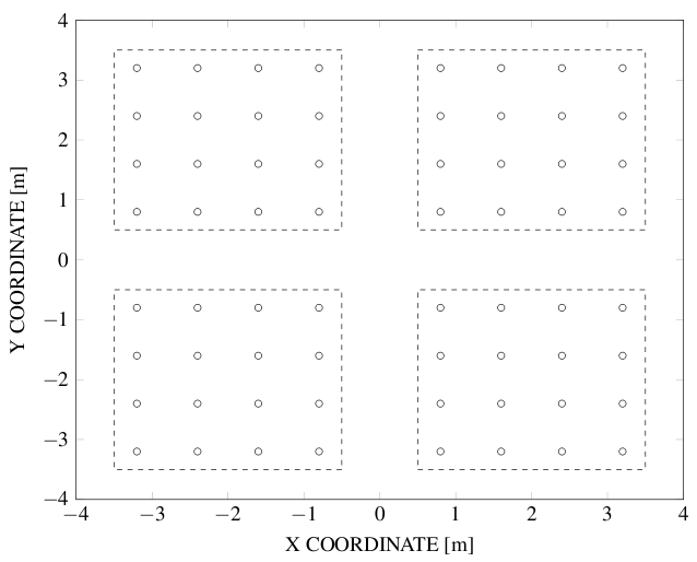
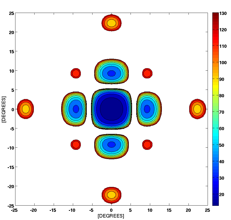
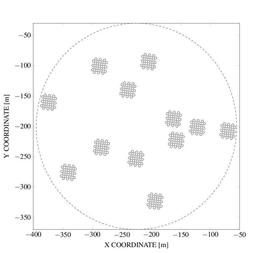
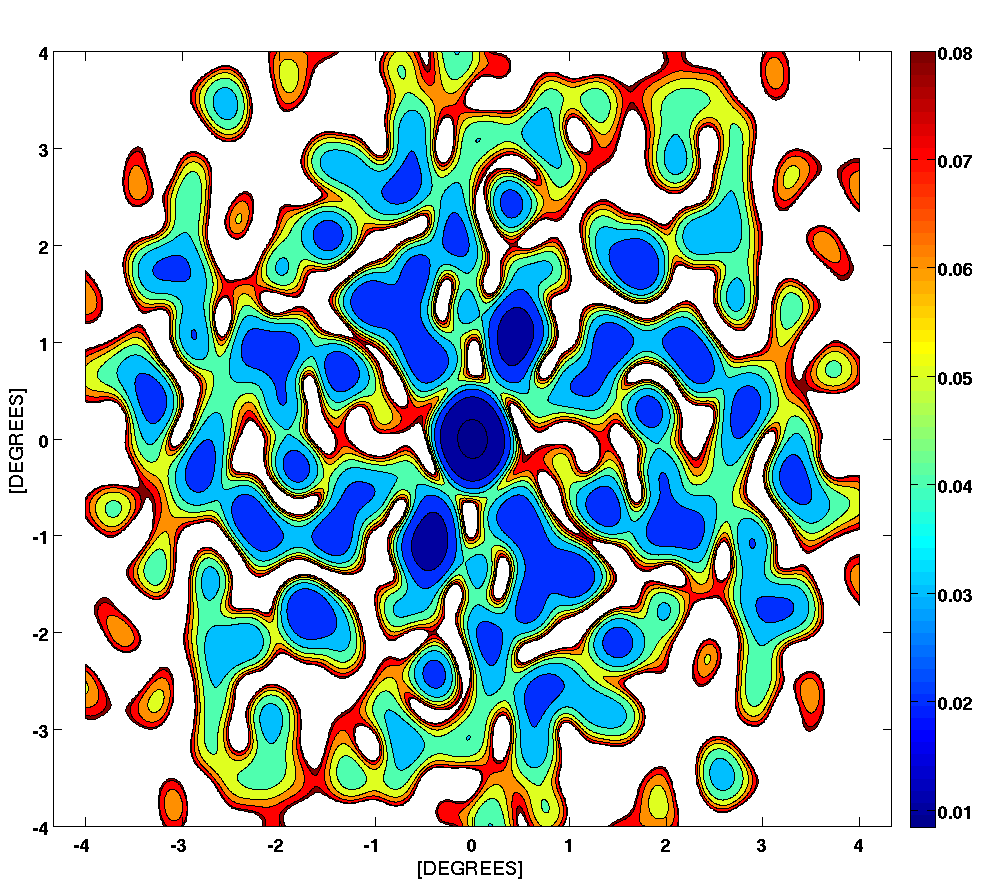
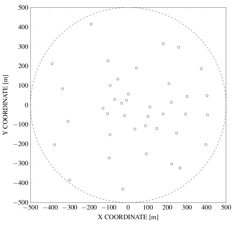
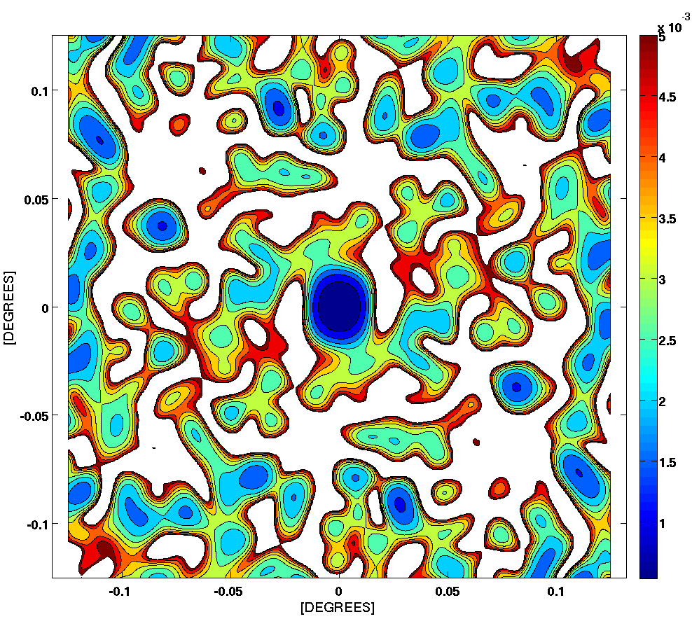
Figure 1: Left column: array configuration and right column sensitivity $\mathscr{S}$ maps, in units of Jy of the MUST, LOFAR and MeerKAT array elements considered here. Top row: the MUST array at 575 MHz; middle row: the LOFAR Superterp at 119 MHz; bottom row: the MeerKAT array core at 1400 MHz. In all cases the antennas are assumed to be pointing at the zenith.

3 Method

The independent TABs of an interferometer can be electronically steered to any direction within the beam of the primary element. They can be arranged into any pattern in the FoV, including Nyquist sampling, in contrast to the fixed beam patterns from horn receivers on single dishes. The TAB gain pattern is, of course, frequency dependent i.e. the beam width gets narrower and sidelobes move closer to the main beam with increasing frequency, as illustrated in Fig. 2. These frequency-dependent variations in a TAB shape can be used to create a sensitivity $\mathscr{S}$ map (a 2-D array in RA and declination) at different frequencies, in particular at the upper $\nu_{H}$ and lower $\nu_{L}$ frequencies in the observing band. To create the sensitivity $\mathscr{S}$ map for each array, the normalised beam patterns, simulated with MATLAB and the more efficient OSKAR-2 package, are scaled to the minimum flux sensitivity $S_{\nu\text{,min}}$ at the phase centre of each TAB. To calculate the minimum flux sensitivity $S_{\nu\text{,min}}$ we used the modified radiometer equation adapted from Lorimer et al. (2006):

$$S_{\nu\text{,min}}=\beta\frac{T\;\left(S/N\right)_{min}}{G\sqrt{n_{p}\tau\Delta\nu}}\>[\text{mJy}]$$ (1)

where G is the effective telescope gain ($\text{K}/\text{Jy}$), $n_{p}$ is the number of polarisations summed, $\Delta\nu$ is the observing bandwidth (MHz), $\tau$ is the integration time (s), T is the system temperature (K), $\left(\text{S}/\text{N}\right)_{min}$ is the minimum signal-to-noise ratio and $\beta$ accounts for digitisation losses and were taken from Kouwenhoven & Voûte (2001). The values used are listed in Table 1.

Sky temperature values vary as a function of Galactic latitude and longitude. To account for that we used the Haslam et al. (1982) 408-MHz all-sky survey. The sky temperature is scaled to the frequencies listed in Table 1 under $\Delta\nu$. The scaling assumes a temperature spectral index of synchrotron radiation of $\alpha$ of -2.6 (Reich & Reich, 1988). The resultant two-dimensional sensitivity maps are plotted in Fig. 1 (right column). We note that we present sensitivities here only as a basis for calculations and that the method actually considers predicted S/Ns and so are simply scaled by any differences in values of the true array from those in Table 1.

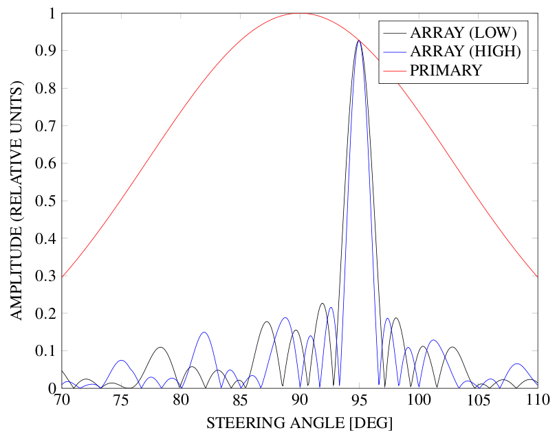
Figure 2: Illustration of the frequency-dependent gain pattern variations for an arbitrary array. The graph depicts a TAB at the lowest frequency (black) and at the highest operational frequency (blue). The fractional bandwidth is $26\%$. The primary beam (red) is plotted only at the lowest frequency for clarity.

Table 1: Values used in Equation 1, where $\beta$ accounts for digitisation losses; $A_{eff}$ is the effective area; $\tau$ is the integration time; $\Delta\nu$ is the observing bandwidth; $n_{p}$ is the number of polarisations summed; $T$ the system temperature given only for the zenith, where the sky temperature $T_{\text{sky}}$ is included in $T$. In addition we list the maximum baseline $B$ and the resulting HPBW at the lowest frequency in the band.

Array	$\beta$	$A_{eff}$	$\tau$	$\Delta\nu$	$n_{p}$	$T$	$B$	HPBWL
		[$m^{2}$]	[s]	[MHz]		[K]	[m]
MUST	0.99	36	$5\times 10^{-3}$	575-625	2	207	5	$5.39^{\circ}$
LOFAR	0.66	8064	$5\times 10^{-3}$	119-150	2	907	300	$0.43^{\circ}$
MeerKAT	0.66	$\sim 5000$	$5\times 10^{-3}$	1400-1700	2	30	1000	$0.52^{\prime}$

The location of a transient source detected with any single-beam radio dish can be constrained only to an area defined by the beam pattern of that dish. In the case of a beam forming interferometer, the source position is most likely to be within the area defined by a HPBW contour of a TAB. This is only a first order assumption as in reality a strong source can be detected anywhere in the beam, including sidelobes. When a source is detected in multiple TABs the resulting detection pattern can be used to approximate the source position to an area smaller than the area of an individual TAB. We will now go on to show that we can use this detection pattern to further constrain the source position even if it was detected in a sidelobe.

The idea is that a pattern of the S/N of the detection of a transient source across the multiple TABs can be generated. From that pattern, corresponding values of the observed (apparent) flux density $S_{\nu}$ can be calculated via Equation 1. The value of the S/N and thus the observed $S_{\nu}$ depends on the source location within a TAB, as the sensitivity decreases away from its phase centre. Fig. 3 illustrates a hypothetical scenario, when three sources are detected in two overlapping TABs at positions marked with A, B and C. Each position is located further away from the phase centre of each TAB. For $\text{TAB}_{1}$, the location C is the most sensitive position and for $\text{TAB}_{2}$ location A is the most sensitive. The resulting ratios of the normalised fluxes from both TABs are then:

$$S_{1A}/S_{2A}=0.24\;\text{,}\;S_{1B}/S_{2B}=0.56\;\;\text{and}\;\;S_{1C}/S_{2C}=0.84,$$

where we have assumed that all fluxes are above the detection threshold. Due to the rapidly changing sensitivity of the TABs away from their phase centres, the flux ratios at each position differ substantially. The ratio of the observed fluxes in the two TABs, $S_{1}/S_{2}$, can be compared with the ratio of the calculated sensitivity across each of TABs, $\mathfrak{s}_{1}/\mathfrak{s}_{2}$, from the beam model and respective sensitivity maps $\mathscr{S}_{1}$ and $\mathscr{S}_{2}$. By identifying the locations where the observed and calculated flux ratios are the same, the source location can be estimated with much higher precision than from a TAB on its own. An example of a flux density ratio $\mathscr{S}_{1}/\mathscr{S}_{2}$ map is shown in Fig. 4 (bottom) for the simple MUST array and the glossary of symbols used is listed in Table 2.

The problem is that the observed $S_{1}/S_{2}$ ratio may not be sufficient to constrain the source location since the calculated $\mathfrak{s}_{1}/\mathfrak{s}_{2}$ ratio can repeat in different areas of the FoV, especially when the inevitable uncertainties are taken into account. Thus another metric is needed.

Table 2: Glossary of symbols used in this paper.

Parameter	Flux density	Spectral index
Observed (1-D)	S	$\alpha$
Map (2-D)	$\mathscr{S}$	$\mathscr{A}$
Map values (1-D)	$\mathfrak{s}$	$\mathfrak{a}$

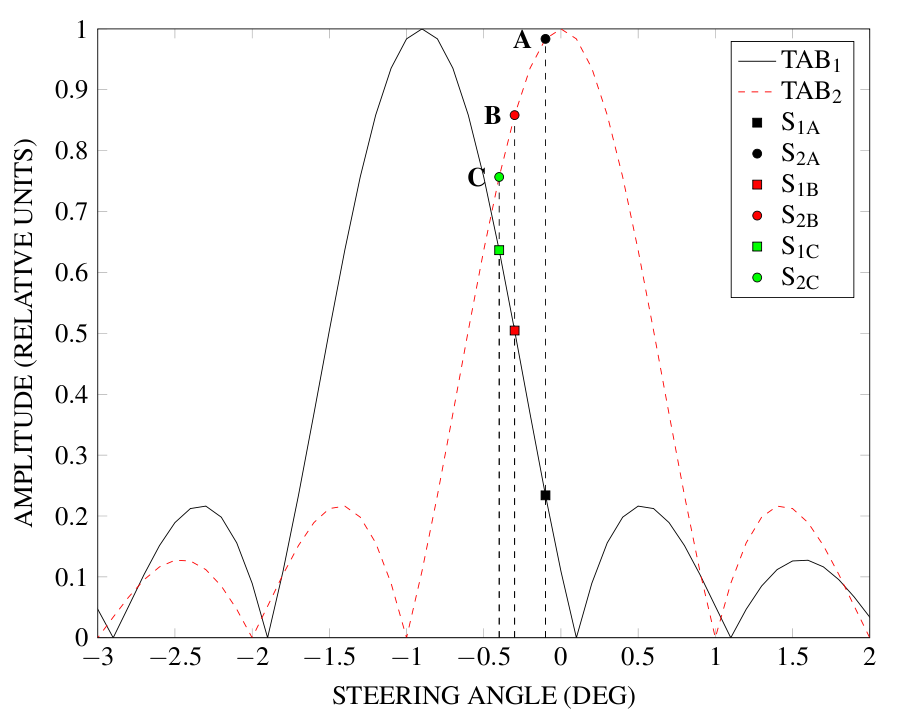
Figure 3: Flux ratios in two overlapping TABs. Three hypothetical strong sources are detected, their positions are marked as A (black), B (red) and C (green). Note that the primary beam shape is not included for clarity. The amplitudes have been normalised to peak at 1.

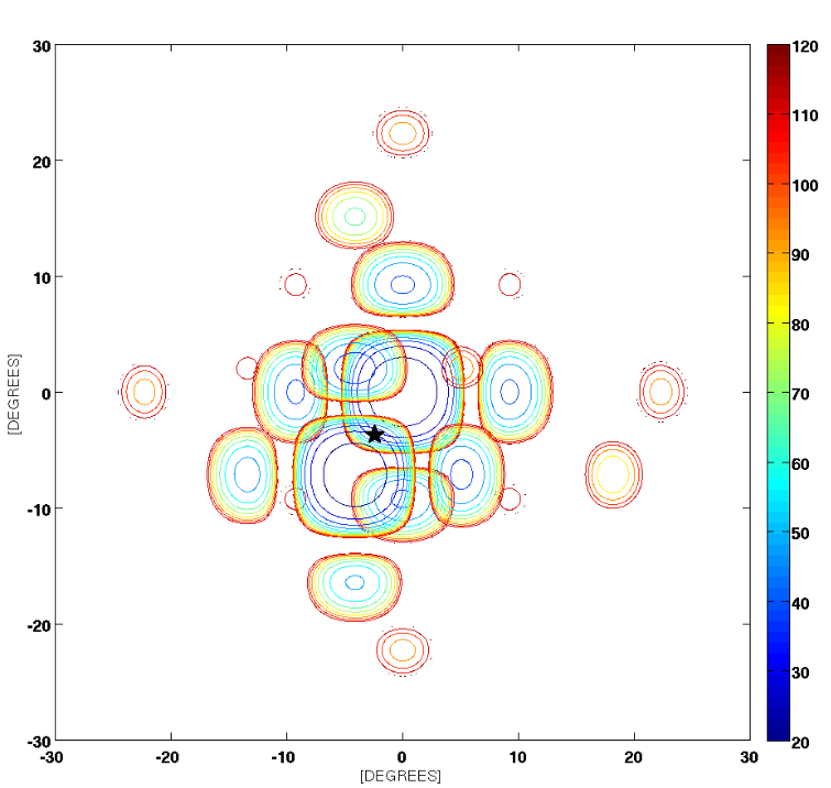
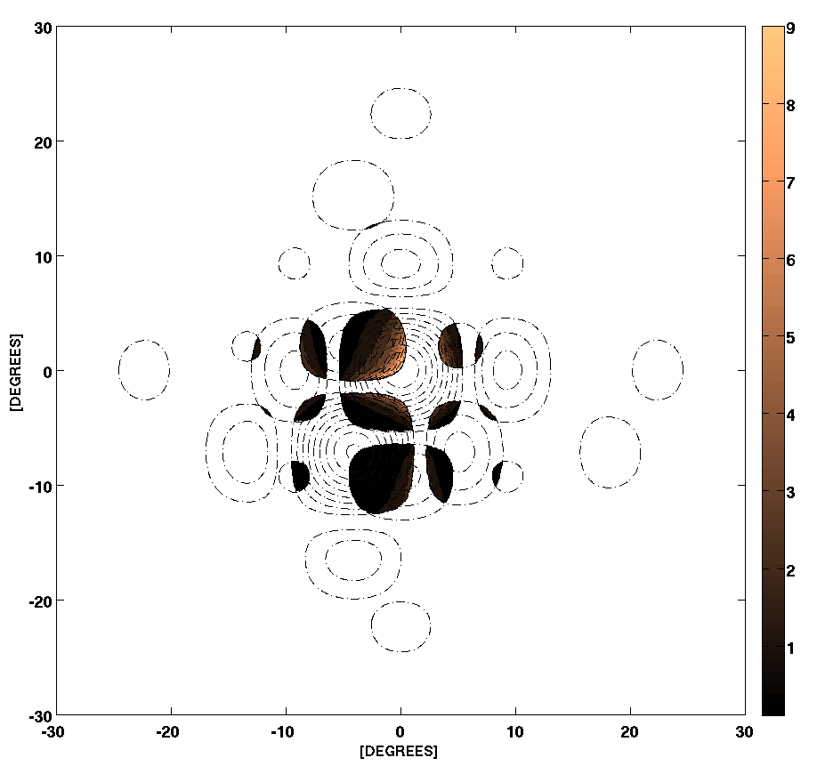
Figure 4: (Top) contour plot of the sensitivity $\mathscr{S}$ maps of two overlapping TABs and their sidelobes of the MUST array in units of Jy. The black star depicts location of a source for a simple example in §3.1. (Bottom) the flux density ratio $\mathscr{S}_{1}/\mathscr{S}_{2}$ map with TAB contours plotted with dashed lines. The flux ratio values are limited to the range $[0.1,10]$ for clarity.

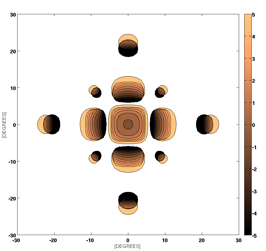
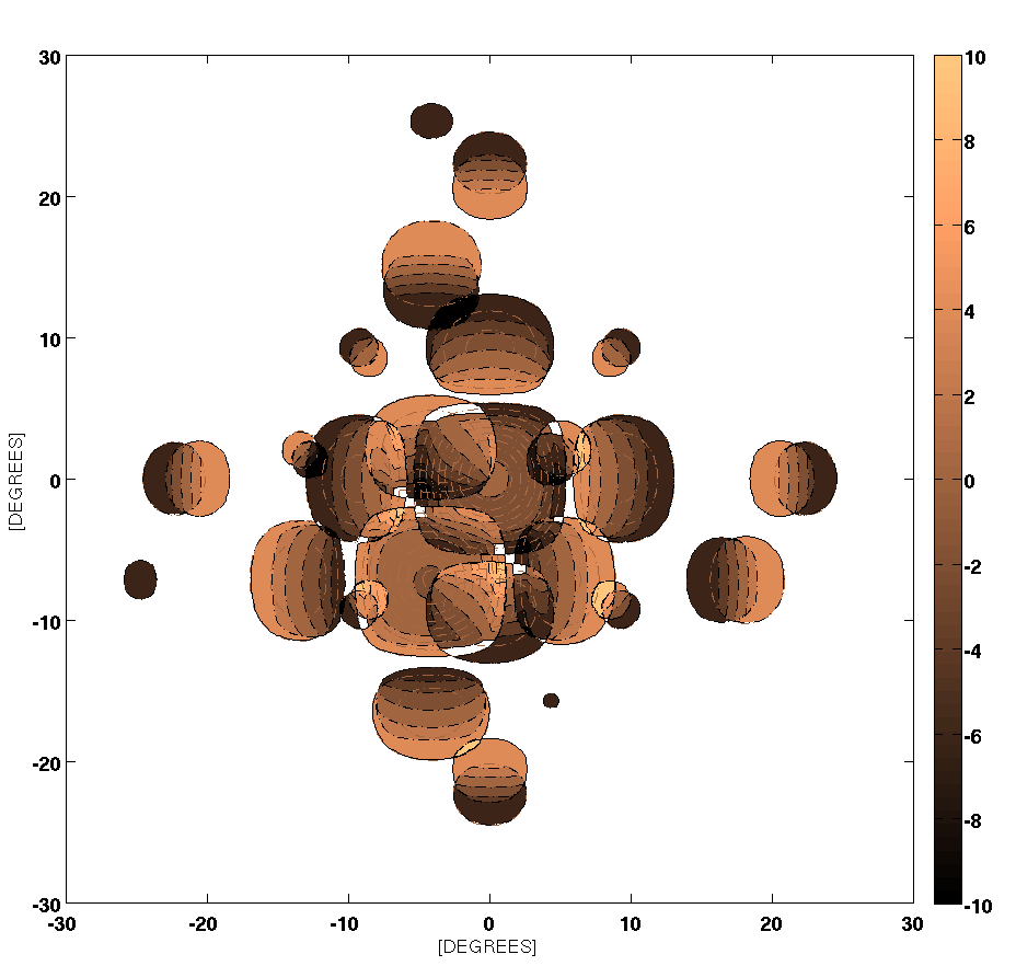
Figure 5: The instrumental spectral index map $\mathscr{A}$ for the MUST array (Top) the values of spectral index are limited to the range $(-5,5)$ and only pixels with sensitivity $10\times S_{\nu\text{,min}}$ are displayed for clarity. (Bottom) the difference spectral index $(\mathscr{A}_{2}-\mathscr{A}_{1})$ map for the MUST array created from the TABs in Fig. 4.

The observed flux density $S_{\nu}$ from many radio sources follows a power law dependency to the first order:

$$S(\nu)\propto\nu^{\alpha},$$ (2)

where $\alpha$ is the spectral index and $\nu$ is the observing frequency. If observations at two distinct frequencies $\nu_{L}$ and $\nu_{H}$ are available, the spectral index $\alpha$ can be calculated using Equation 2 as:

$$\alpha=\frac{\log\left({\frac{S_{L}}{S_{H}}}\right)}{\log\left({\frac{\nu_{L}}{\nu_{H}}}\right)},$$ (3)

where $S_{L}$ and $S_{H}$ are the apparent flux densities from observations at frequencies $\nu_{L}$ and $\nu_{H}$. We note that when calculating these sensitivities, we have assumed the full bandwidth given in Table 1 for each of $\nu_{L}$ and $\nu_{H}$. That is, $\nu_{L}$ and $\nu_{H}$ are the centres of these bands. As discussed in Section 5 a subsequent analysis should include the fact that $S_{L}$ and $S_{H}$ represent average values. As above we note that the accuracy of our values for $S_{L}$ and $S_{H}$ do not affect the efficacy of our method. Due to the frequency-dependent gain pattern of a TAB, sources detected off-axis can have their spectral indices distorted substantially. In our analysis we have assumed that the beam dependent spectral index is also described by a power law. To investigate this effect further, we use Equation 3 and 2-D sensitivity $\mathscr{S}$ maps for frequencies $\nu_{L}$ and $\nu_{H}$, to create a 2-D instrumental spectral index, $\mathscr{A}$, map of a telescope beam pattern, as illustrated in Fig. 5 (top) for the MUST array.

In contrast to Spitler et al. (2014), the instrumental spectral index $\mathscr{A}$ map is created using the sensitivity (Equation 1) of the beam at a given observing frequency rather than its gain. This is in order to include the noise contribution from the sky. The apparent variation of the instrumental spectral index away from the phase centre therefore has the opposite sign to that of Spitler et al. (2014). We assume that the observed spectral index $\alpha_{O}$ of a detected source is a combination of its intrinsic spectral index $\alpha_{I}$ and the calculated instrumental spectral index $\mathfrak{a}$ imposed by the beam patterns. It can thus be described with the simple equation:

$$\alpha_{I}=\alpha_{O}+\mathfrak{a}$$ (4)

Using Fig. 3 as an illustration again, a source observed at position A, with normalised flux density $S_{1A}$ from $\text{TAB}_{1}$ and $S_{2A}$ from $\text{TAB}_{2}$, is also detected at both frequencies, $\nu_{L}$ and $\nu_{H}$, yielding four different values of flux density. $S_{1A,\nu_{L}}$ and $S_{1A,\nu_{H}}$ for $\text{TAB}_{1}$ and $S_{2A,\nu_{L}}$ and $S_{2A,\nu_{H}}$ for $\text{TAB}_{2}$. Using Equation 3 we can calculate the observed spectral index $\alpha_{O_{1}}$ for source A detected in $\text{TAB}_{1}$ and $\alpha_{O_{2}}$ for source A detected in $\text{TAB}_{2}$. As both TABs detected the same source A, Equation 4 can be written as follows (omitting subscript A for clarity):

$$\alpha_{O_{1}}=\alpha_{I}-\mathfrak{a}_{1},$$

$$\alpha_{O_{2}}=\alpha_{I}-\mathfrak{a}_{2}.$$ (5)

These two equalities yield the relationship:

$$\alpha_{O_{1}}-\alpha_{O_{2}}=\mathfrak{a}_{2}-\mathfrak{a}_{1},$$ (6)

and the left side of this equality is known from the detections. To connect the calculated difference $(\mathfrak{a}_{2}-\mathfrak{a}_{1})$ to a position within a TAB we need to subtract the instrumental spectral index $\mathscr{A}_{2}$ map of $\text{TAB}_{2}$ from the instrumental spectral index $\mathscr{A}_{1}$ map of $\text{TAB}_{1}$. An example of such manipulation is illustrated in Fig. 5 (bottom) for the MUST array. At any point the difference of the observed spectral indices $(\alpha_{O_{1}}-\alpha_{O_{2}})$ together with the observed flux density ratio $S_{1}/S_{2}$, can be used to constrain the position of a source within the two TABs with an accuracy significantly better than a beam width. The symbols used in relation to the spectral index manipulations are also summarised in Table 2.

The above two-TAB detection analysis of the observed flux density ratio and spectral index difference produces a single or a set of possible locations for a source. If a transient source was detected in N TABs, this process can be repeated for all $N(N-1)/2$ pair combinations. To identify the pair combinations we will use subscripts $(i,\;j)$. The final step in the process is to compare the estimated locations resulting from all the TAB pairs against each other. Only locations common for all pairs are chosen for the estimated true source position. This is illustrated in Fig. 6, for a source detected in five TABs that Nyquist sample the FoV, where each colour depicts overlapping regions of $(\mathfrak{s}_{1}/\mathfrak{s}_{2})_{(i,\;j)}$ and $(\mathfrak{a}_{2}-\mathfrak{a}_{1})_{(i,\;j)}$ from each TAB pair. For example, orange represents overlapping regions of $(\mathfrak{s}_{1}/\mathfrak{s}_{2})_{(11,\;17)}$ and $(\mathfrak{a}_{2}-\mathfrak{a}_{1})_{(11,\;17)}$ for the $\text{TAB}_{11}$ and $\text{TAB}_{17}$ pair. Crucially, only regions where all ”colours” overlap are treated as a possible source location. A simplified example is also given in §3.1.

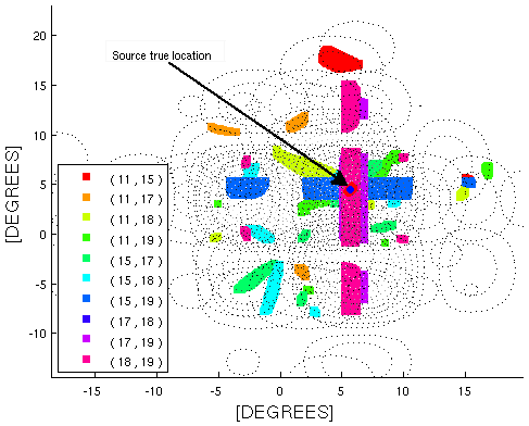
Figure 6: Illustration of a detection made with five TABs that Nyquist sample the FoV resulting in $C_{2}^{5}=10$ pair combinations. Each colour depicts overlapping regions of $(\mathfrak{s}_{1}/\mathfrak{s}_{2})_{(i,\;j)}$ and $(\mathfrak{a}_{2}-\mathfrak{a}_{1})_{(i,\;j)}$ from each $(i,\;j)$ TAB pair.

To summarise, our analysis we only consider sources that were detected:

1. in at least two TABs and

2. at two frequencies, $\nu_{L}$ and $\nu_{H}$ in each TAB.

In reality a source could be detected in just one beam or at one frequency only. Hence, our definition of detection is quite restrictive but is required to provide better positional accuracy. A by-product of an accurate position estimation is the possibility of recovering the intrinsic spectral index $\alpha_{I}$ of a source. Since our main assumption is that a telescope imparts deterministic instrumental spectral index to a detected source, the latter can be corrected for if the position of the source within a TAB is known.

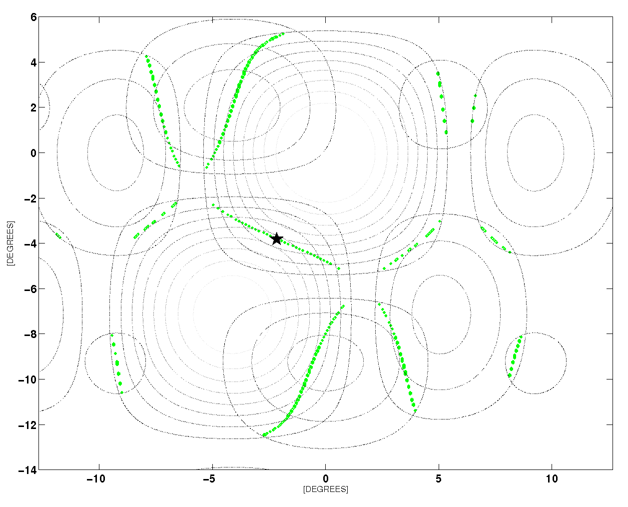
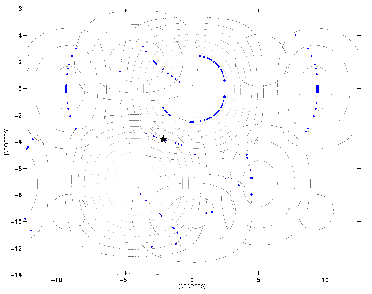
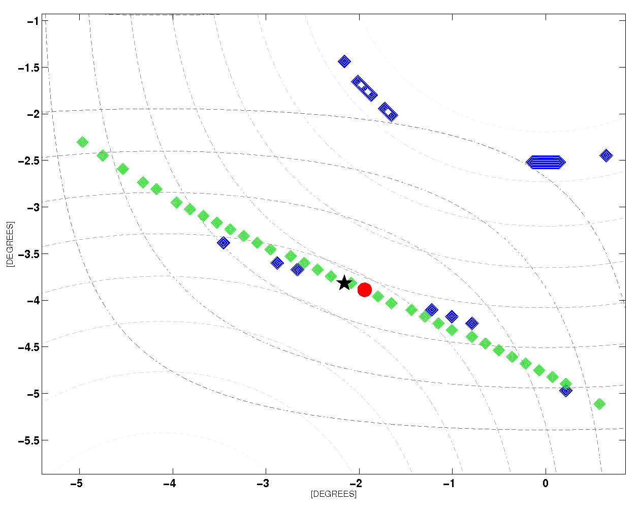
Figure 7: A hypothetical source was detected in two overlapping MUST TABs at a position $[-2.1^{\circ},-3.8^{\circ}]$, depicted as a black star. The top figure shows the values of $\mathfrak{s}_{1}/\mathfrak{s}_{2}=S_{1}/S_{2}\pm 1\%$, plotted on top of the TAB contours. The middle figure shows values of $(\mathfrak{a}_{2}-\mathfrak{a}_{1})=(\alpha_{O_{1}}-\alpha_{O_{2}})\pm 1\%$. The bottom figure shows both $(\mathfrak{a}_{2}-\mathfrak{a}_{1})$ and $\mathfrak{s}_{1}/\mathfrak{s}_{2}$ overlaid. The red dot at a position $[-1.95^{\circ},-3.9^{\circ}]$ indicates the best estimated position.

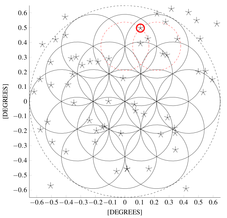
Figure 8: A schematic of Nyquist sampled LOFAR TABs which illustrates the general layout assumed in all simulations. Black circles represent a 3-dB contour of a TAB at the lower frequency $\nu_{L}$ in the observing band. The dashed circle represents the TAB test area and stars depict positions of randomly generated sources. Two red circles represent a 3-dB contour of a TAB at the higher frequency $\nu_{H}$ of the observing band.

3.1 Simple Example

In Fig. 7 we graphically illustrate the methodology of finding a source location using the observed S/N pattern for the MUST array. We simulated a source at the position $[-2.1^{\circ},-3.8^{\circ}]$ from the assumed FoV centre in two overlapping TABs. This is marked with a black star in Fig. 4 (top) and in Fig. 7. The source was detected in two TABs and at $\nu_{H}$ and $\nu_{L}$ fulfilling both requirements of our restrictive definition of detection. As we are demonstrating only a simple two TAB detection the subscripts $(i,\;j)$ are omitted here. The observed S/N pattern yields $\text{S}_{1}/\text{S}_{2}$ = 0.86 and $(\alpha_{O_{1}}-\alpha_{O_{2}})$ = - 0.52, for the observed flux density ratio and the observed spectral index difference respectively. In this first illustration of the technique we consider first only modest errors $(\pm 1\%)$ on the calculated values of $\mathfrak{s}_{1}/\mathfrak{s}_{2}$ and $(\mathfrak{a}_{2}-\mathfrak{a}_{1})$ and do not include any statistical error propagation for ease of presentation. A further error discussion is included below while a detailed analysis will be given in a later paper.

Fig. 7 (top) shows the repeating values of $\mathfrak{s}_{1}/\mathfrak{s}_{2}=S_{1}/S_{2}\pm 1\%$ from the 2-D flux density ratio $\mathscr{S}_{1}/\mathscr{S}_{2}$ map. The repeating regions of $\mathfrak{s}_{1}/\mathfrak{s}_{2}$ from the TAB pairs are indicated by the colour green and the TAB contours are plotted as well to guide orientation. Fig. 7 (middle) shows, plotted in blue, the repeating values of $(\mathfrak{a}_{2}-\mathfrak{a}_{1})=(\alpha_{O_{1}}-\alpha_{O_{2}})\pm 1\%$ obtained from the 2-D instrumental spectral index difference $(\mathscr{A}_{2}-\mathscr{A}_{1})$ map. If we overlay the top and the middle panel, as in Fig. 7 (bottom), we can establish a position where both these allowed regions, $(\mathfrak{a}_{2}-\mathfrak{a}_{1})$ and $\mathfrak{s}_{1}/\mathfrak{s}_{2}$, overlap. Only those values that share the same coordinates are treated as a possible source location. In our example, there is only one common coordinate, for both values of $(\mathfrak{a}_{2}-\mathfrak{a}_{1})$ and $\mathfrak{s}_{1}/\mathfrak{s}_{2}$, which lies at $[-1.95^{\circ},-3.9^{\circ}]$, and thus is marked with a red dot in Fig. 7 (bottom). By this means we were able to estimate the source location to within $0.02$ HPBW_L of a TAB from the true source position marked with a black star in Fig. 7 (bottom). For example, for the LOFAR array an accuracy of $0.02$ HPBW_L signifies 0.5 arcminute distance from the true source position, whereas for MeerKAT the same distance signifies one arcsecond. By increasing the assumed error on the calculated $\mathfrak{s}_{1}/\mathfrak{s}_{2}$ ratios and the $(\mathfrak{a}_{2}-\mathfrak{a}_{1})$ differences with a two TAB detection, the number of estimated positions will increase. For example, a $5\%$ error on both the ratio and the difference results in four additional estimated locations. However, as is shown later in the text, even considerable errors still allow a useful location estimation if a source is detected with several TABs treated in a pairwise fashion.

3.2 Error considerations

In the simplified example just shown we assumed highly significant detections (i.e. S/N of 100) simply to illustrate the method. These do not reflect likely S/Ns in actual observations so here we consider that, to qualify as a detection, a transient source must have S/N $\geqslant 8$ and thus a related flux error of $\delta S\leqslant 12.5\%$. The question of whether the errors between TABs are correlated or independent is non-trivial, being a combination of several factors. For example there may be a degree of non-independent noise, depending on the relative contribution of the sky and receiver temperatures; these will be quite different in the LOFAR and MeerKAT arrays. We will address the issue of sources of errors and their treatment in a later paper. For the present discussion we consider the worst case scenario for all three arrays where the errors taken to be highly correlated and hence combine linearly rather than quadratically. However, for comparison, we also show the results from considering the errors to be independent for the MeerKAT core (Table 5). It has good range of baselines and is dominated by the receiver noise at the assumed frequency of 1.4 GHz.

The error $\delta(S_{1}/S_{2})_{\nu}$ on the observed flux density ratio $(S_{1}/S_{2})$ comes from the S/N of the TAB detections, i.e.:

$$\delta(S_{1}/S_{2})_{\nu}=\left(\frac{\delta S_{1}}{S_{1}}+\frac{\delta S_{2}}{S_{2}}\right)_{\nu}.$$ (7)

The observed $(S_{1}/S_{2})$ and the modelled $\mathfrak{s}_{1}/\mathfrak{s}_{2}$ ratios, obtained from the 2-D flux density ratio $\mathscr{S}_{1}/\mathscr{S}_{2}$ map, can then be compared. We are looking for regions where the modelled $\mathfrak{s}_{1}/\mathfrak{s}_{2}$ falls within the range:

$$S_{1}/S_{2}\pm\delta(S_{1}/S_{2}).$$ (8)

For the sources simulated in this study, the cumulative error on the flux ratio $(S_{1}/S_{2})$ is typically $\pm 20\%$.

The measured flux densities are is also used via Equation 3 to estimate the observed spectral index $\alpha_{O}$. The cumulative error $\delta\alpha_{O}$ is calculated as follows:

$$\delta\alpha_{O}=\frac{0.43}{\log\left({\frac{\nu_{L}}{\nu_{H}}}\right)}\left(\frac{\frac{\delta S_{\nu_{L}}}{S_{\nu_{L}}}+\frac{\delta S_{\nu_{H}}}{S_{\nu_{H}}}}{\frac{S_{\nu_{L}}}{S_{\nu_{H}}}}\right).$$ (9)

The error then propagates further as we are considering the observed spectral index difference from two TABs (Equation 6):

$$\delta(\alpha_{O_{2}}-\alpha_{O_{1}})=\delta\alpha_{O_{2}}+\delta\alpha_{O_{1}}.$$ (10)

The calculated $(\alpha_{O_{2}}-\alpha_{O_{1}})$ and modelled $(\mathfrak{a}_{2}-\mathfrak{a}_{1})$, from the 2-D the spectral index difference $(\mathscr{A}_{2}-\mathscr{A}_{1})$ map, are then compared, we are looking for regions where the modelled $(\mathfrak{a}_{2}-\mathfrak{a}_{1})$ falls within the range:

$$(\alpha_{O_{2}}-\alpha_{O_{1}})\;\pm\;\delta(\alpha_{O_{2}}-\alpha_{O_{1}}).$$ (11)

The cumulative error on the spectral index difference $\delta(\alpha_{O_{2}}-\alpha_{O_{1}})$ is typically large in our simulations. It is at least $60\%$ and for the present purpose we have limited the error to $100\%$. It is important to note that these error refer only to the simulated sources presented in this work and are not generic to the method. These errors can be reduced with large fractional bandwidths but that can make a detection at two frequencies difficult.

3.3 Simulation Parameters

To explore the capabilities of our method, we tested three different spatial sampling methods to determine how important the TAB separation is for the accuracy of determining a source location. We first consider the case where the TABs undersampled the FoV. This means that TABs touch at the $\text{HPBW}_{L}$ contour at the lowest observing frequency $\nu_{L}$. In the second case, the TABs Nyquist sample the FoV i.e. the separation between the phase centres of TABs is equal to $\text{HPBW}_{L}/2$ at the lower edge of the observed frequency band. Of course Nyquist sampling at $\nu_{L}$ means undersampling at $\nu_{H}$. In the third case, the TABs oversample the FoV i.e. the TABs are Nyquist sampled at the highest frequency ($\text{HPBW}_{H}/2$). Oversampling is used as a control to determine if there are any significant benefits from a high surface density of TABs.

Fig. 8 shows an example of the generic test setup used in the analysis. We only show the case of Nyquist-sampled TABs as this layout is similar for all arrays. Fig. 8 also shows a 3-dB contour of a TAB at the higher frequency $\nu_{H}$ in the LOFAR Superterp observing band to illustrate the undersampling at $\nu_{H}$. The independent TABs are simulated to occupy a circle with a diameter equal to $3\times\text{HPBW}_{L}$. The centre of the circle is located at the zenith for each telescope’s geographical location and for a specific MJD. A set of 60 strong point sources, all with $\alpha_{I}$ equal to -2, is randomly distributed in a square of side equal to $3\times\text{HPBW}_{L}$ encompassing the TABs. The predicted detection significance at the TAB centre is taken to be $20\sigma$ for each source at $\nu_{L}$ and scaled by the spectral index to obtain the flux density at $\nu_{H}$. We then calculated the TAB sensitivities using Equation 1.

In our simulations we have assumed a perfectly calibrated array where all the antenna gains are uniform and our beam model is ideal. In a real telescope, each antenna will have uncalibrated errors in gain and phase. This inevitably will affect the performance of our method, but for this proof-of-concept analysis we assume perfect calibration. In Section 5 we identify several other practical issues which will need to be quantified in a real-life application of this method.

4 Results

To present the results of our simulations in a compact form, we divided the data according to how many locations m were estimated per detected source. Location is used to describe a region where the true source position might be. For the purpose of illustration, Fig. 9 is a schematic showing estimated locations for a hypothetical source A with $m=2$ and a source B with $m=3$. Table 3 lists sources for which the number of estimated locations m is between 1 and 5 and also a group containing all detections with more than 5 estimated locations. For the number of sources n in each location group we calculated the mean number of TABs ($\overline{B}$) in which the source was detected to illustrate the benefits of detection with many TABs. Next we list the minimum ($\delta D_{Min}$), maximum ($\delta D_{Max}$) and mean ($\overline{D}$) value of the total area D covered by the overlapping values of $\mathfrak{s}_{1}/\mathfrak{s}_{2}$ and $(\mathfrak{a}_{2}-\mathfrak{a}_{1})$, normalised to the TAB’s solid angle $\Omega_{HPBW_{L}}$ at $\nu_{L}$. The total area D represents the area that would need to be sampled in follow-up, or archival, observations to be sure that the actual position of the source was observed. In our simulations, the smallest D is represented by a single pixel, i.e. the smallest resolution element of the simulated beam pattern. A single pixel covers an area of $0.32$ square arcmin for the MUST array, $0.23$ square arcsec for the LOFAR Superterp and $2.25\times 10^{-4}$ square arcsec for MeerKAT.

In Fig. 9 it is clear that the total area $\delta D_{B}$ for a source B is considerably larger than the total area $\delta D_{A}$ for source A. However, the total area $\delta D_{B}$ is condensed to mostly a single patch. Out of the two, the location estimated for source A has lower uncertainty as there are only two estimated locations and $\overline{D}$ is smaller than for source B.

In Table 3 we also list the minimum ($\delta\phi_{Min}$), maximum ($\delta\phi_{Max}$) and mean ($\overline{\Delta\phi}$) value of the total angular distances $\Delta\phi$ between the true and the estimated source positions, normalised to the HPBW_L. We illustrate the above using an example from column two in Table 3, for the MeerKAT array using the Nyquist sampled method; two patches (m) were estimated for three sources (n) with a mean number of TABs ($\overline{B}$) equal to three. The maximum angular distance $\delta\phi_{max}$ for a detection in this group is 6.3 HPBW_L away from the true position but the mean area $\overline{D}$ to survey for possible host galaxies is only 0.12 of the $\Omega_{HPBW_{L}}$ area. This would suggest a similar scenario to source A (small $\overline{D}$ and large $\delta\phi_{max}$) in Fig. 9.

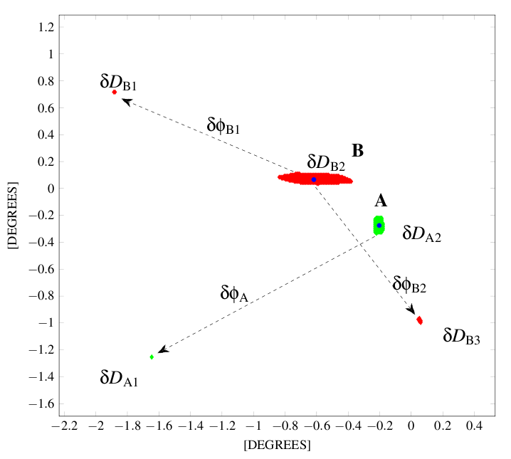
Figure 9: Schematic representation of locations m, the total area D and the angular distance $\delta\phi$ from the true source position, marked with blue dot. The green patches ($m=2$) represent the two estimated locations for source A. Red patches ($m=3$) represent the three estimated locations for source B. While there may be a significant angular distance between the estimated locations, the areas to search at these locations may be quite small.

We now review the overall statistics of the results starting with the detection rates. We then give examples of detections with low and high positional uncertainty, followed by an estimation of the accuracy of recovery of the true source position. We finish by presenting the results of the intrinsic spectral index recovery.

4.1 Detection Rates

The number of detected sources that meet our two criteria for detection, are summarised in Table 4. For the LOFAR and MeerKAT arrays with large fractional bandwidths (23$\%$ and 19$\%$ respectively) the undersampling of the FoV yields the lowest detection rate of two and three sources out of 60 respectively. This is not unexpected as the first condition for detection is difficult to meet without overlapping TABs. For the MUST array, with strong regular sidelobes and small fractional bandwidth of 8$\%$, the undersampling of the FoV yields a detection of 14 out of 60 random sources. Because of our restrictive definition of detection and due to the low detection rates for the LOFAR and the MeerKAT arrays, we will no longer consider the results from the undersampling method.

Sampling of the FoV with the Nyquist-sampled TABs increased the detection rates dramatically for all arrays. The biggest change is observed for the LOFAR array which detected 48 sources. The lowest detection rate is achieved with the MeerKAT array at only 33 sources out of 60 sources. As discussed below this is likely due to the high fractional bandwidth, as illustrated in Fig. 8. This effect is not replicated in LOFAR, with similar fractional bandwidth, due to the presence of strong sidelobes, as illustrated in Fig. 1.

Fig. 10 shows a representation of sources detected using different sampling methods for the LOFAR TABs. All undetected sources ($\Diamond$) lay outside of the TAB test area. But some sources that lie outside of the test area were detected with the oversampling of the FoV. A source marked with a red circle in Fig. 10 and in Fig. 8, illustrates the impact of fractional bandwidth on the detection rates. Fig. 8 shows the Nyquist sampled FoV with the LOFAR TABs at the lower frequency $\nu_{L}$ (black circles), where two contours of TABs at the higher frequency $\nu_{H}$ in the observing band are also shown (red circles). The marked source is not detected when the FoV is Nyquist sampled as the second condition for successful detection is not satisfied. For simplicity our simulations considered only two frequencies, at the extremes of the bandwidth. The detection rate could be improved by considering many sub-bands and in a future paper we plan to discuss how this would, in turn, improve the location accuracy.

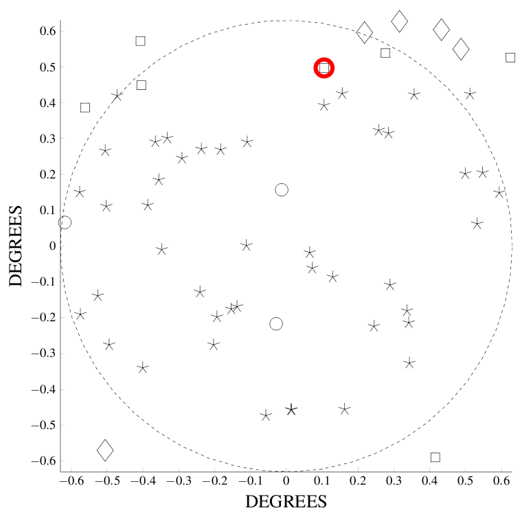
Figure 10: Graphical representation of sources detected using different sampling methods for the LOFAR Superterp TABs. Black circle: sources detected with undersampling, Nyquist sampling and oversampling. Star: sources detected with Nyquist sampling and oversampling. Diamond: no detection with any sampling method. Square: sources detected with oversampling only.

Table 3: Comparison of the accuracy of the Nyquist sampled and oversampled methods for determining the positions and the intrinsic spectral index. Here m is the number of locations estimated per detected source. n is the number of sources detected at the number of positions shown. $\overline{B}$ is the mean number of TABs per source. Below we list the minimum ($\delta D_{Min}$), maximum ($\delta D_{Max}$) and mean ($\overline{D}$) value of the total area D covered by the overlapping values of $\mathfrak{s}_{1}/\mathfrak{s}_{2}$ and $(\mathfrak{a}_{2}-\mathfrak{a}_{1})$, normalised to the $\Omega_{HPBW_{L}}$ area in deg². The total area D represents the area that would need to be sampled in follow up, or archival, observations to be sure that the actual position of the source was observed. We also list the minimum ($\delta\phi_{Min}$), maximum ($\delta\phi_{Max}$) and mean ($\overline{\Delta\phi}$) value of the total angular distances $\Delta\phi$ between the true and the estimated source position, normalised to the HPBW_L. $\overline{\alpha_{I}}$ is the mean estimated intrinsic spectral index of all sources from group m where $\sigma$ is the standard deviation from that mean.

		MUST
Parameter		Nyquist sampling						Oversampling
m		1	2	3	4	5	¿5		1	2	3	4	5	¿5
n		33	1	3	1	1	1		30	4	1	-	1	4
$\overline{B}$		5	2	2	3	2	8		6	3	3	-	2	6
D
	$\delta D_{Min}$	0.00045	0.084	0.00023	0.00023	0.043	0.00023		0.00023	0.00023	0.00023	-	0.00023	0.00023
	$\delta D_{Max}$	1.4	0.25	1.5	0.062	0.73	0.00023		0.42	1.6	0.03	-	0.6	0.8
	$\overline{D}$	0.08	0.17	0.30	0.02	0.41	0.00023		0.05	0.28	0.01	-	0.20	0.07
$\delta\phi$
	$\delta\phi_{Min}$	0.00062	0.0018	0.0038	0.0052	0.0035	0.052		0.0012	0.0010	0.0018	-	0.0024	0.0017
	$\Delta\phi_{Max}$	0.7	1.6	1.6	0.2	3.5	1.6		0.4	1.7	0.8	-	3.1	2.2
	$\overline{\Delta\phi}$	0.04	0.65	0.25	0.08	1.3	0.72		0.04	0.22	0.05	-	0.70	0.60
$\alpha_{I}$
	$\overline{\alpha_{I}}$	-2.0	-2.3	-1.8	-2.0	-1.5	-0.3		-1.9	-2.1	-2.0	-	-0.9	-0.8
	$\sigma$	0.2	1.0	0.8	0.6	1.7	2.5		0.3	0.5	0.4	-	1.8	1.8
		LOFAR
Parameter		Nyquist sampling						Oversampling
m		1	2	3	4	5	¿5		1	2	3	4	5	¿5
n		7	6	4	3	2	26		24	6	1	3	2	19
$\overline{B}$		4	3	3	3	3	3		5	4	5	3	3	3
D
	$\delta D_{Min}$	0.0004	0.0004	0.0004	0.0004	0.0004	0.0004		0.0004	0.0004	0.0004	0.0004	0.0004	0.0004
	$\delta D_{Max}$	0.6	0.6	1.1	0.3	0.7	2.9		0.4	0.1	0.0004	0.8	0.2	1.6
	$\overline{D}$	0.09	0.08	0.2	0.05	0.09	0.07		0.03	0.03	0.0004	0.14	0.03	0.07
$\delta\phi$
	$\delta\phi_{Min}$	0.006	0.004	0.007	0.003	0.007	0.002		0.002	0.004	0.003	0.004	0.004	0.003
	$\delta\phi_{Max}$	1.3	4.1	3.7	3.8	3.9	8		0.7	2.9	0.04	3.6	3.8	8.1
	$\overline{\Delta\phi}$	0.09	0.6	0.5	0.4	0.6	1.6		0.05	0.4	0.03	0.6	0.6	1.7
$\alpha_{I}$
	$\overline{\alpha_{I}}$	-2	-1.8	-1.5	-1.8	-1.7	-1.1		-2	-2	-2	-1.6	-1.8	-1.3
	$\sigma$	0.12	0.3	0.6	0.3	0.6	1.1		0.07	0.15	0.09	0.7	0.25	0.8
		MeerKAT
Parameter		Nyquist sampling						Oversampling
m		1	2	3	4	5	¿5		1	2	3	4	5	¿5
n		25	3	1	2	-	2		38	2	1	-	1	1
$\overline{B}$		4	3	3	3	-	2		5	3	6	-	2	2
D
	$\delta D_{Min}$	0.0004	0.0004	0.0008	0.0004	-	0.0004		0.0004	0.0015	0.0004	-	0.0008	0.0004
	$\delta D_{Max}$	2.1	0.6	0.07	2.3	-	2.1		1.9	2.5	0.0004	-	1.1	1.1
	$\overline{D}$	0.12	0.12	0.03	0.31	-	0.21		0.11	0.63	0.0004	-	0.23	0.14
$\delta\phi$
	$\delta\phi_{Min}$	0.001	0.002	0.009	0.007	-	0.007		0.001	0.004	0.007	-	0.008	0.002
	$\delta\phi_{Max}$	1.3	6.3	9.9	10	-	11		1.4	6.1	0.04	-	11	11
	$\overline{\Delta\phi}$	0.08	1.3	0.54	0.66	-	1.1		0.06	0.36	0.03	-	0.69	0.86
$\alpha_{I}$
	$\overline{\alpha_{I}}$	-1.9	-1.1	-1.8	-1.5	-	-0.9		-2	-1.7	-2	-	-1.2	-1.1
	$\sigma$	0.1	1.5	0.6	0.8	-	1.2		0.07	0.5	0.05	-	1	1.1

4.2 Example Detection

In Fig. 11 we present examples of the estimated source positions for representative cases with low (one location only) and high (many possible locations) positional uncertainty for the MUST array, the LOFAR array and the MeerKAT array. These also span the range of spatial sampling methods.

Each panel in Fig. 11 is a simplified version of Fig. 6 which showed a detection made with five TABs for illustration only. We use only green squares in Fig. 11 instead to represent overlapping regions from TAB pairs, within the uncertainty calculated as described in §3.2. The red regions show the common intersection between all TAB pairs. The blue circles indicate the true position of a source, noting that in some cases it obscures the red region. The contours of $\mathscr{S}$ for each of the TABs where a detection was made are also plotted.

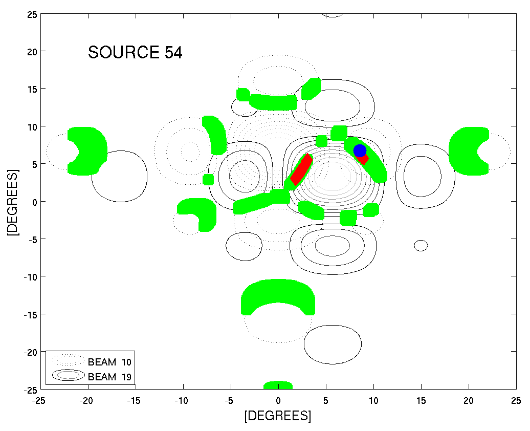
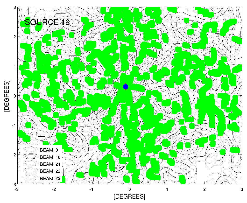
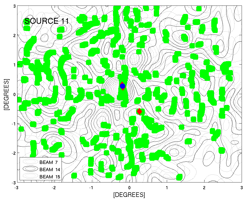
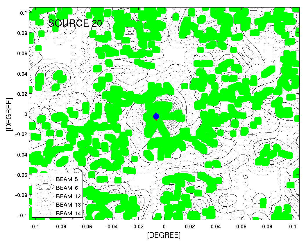
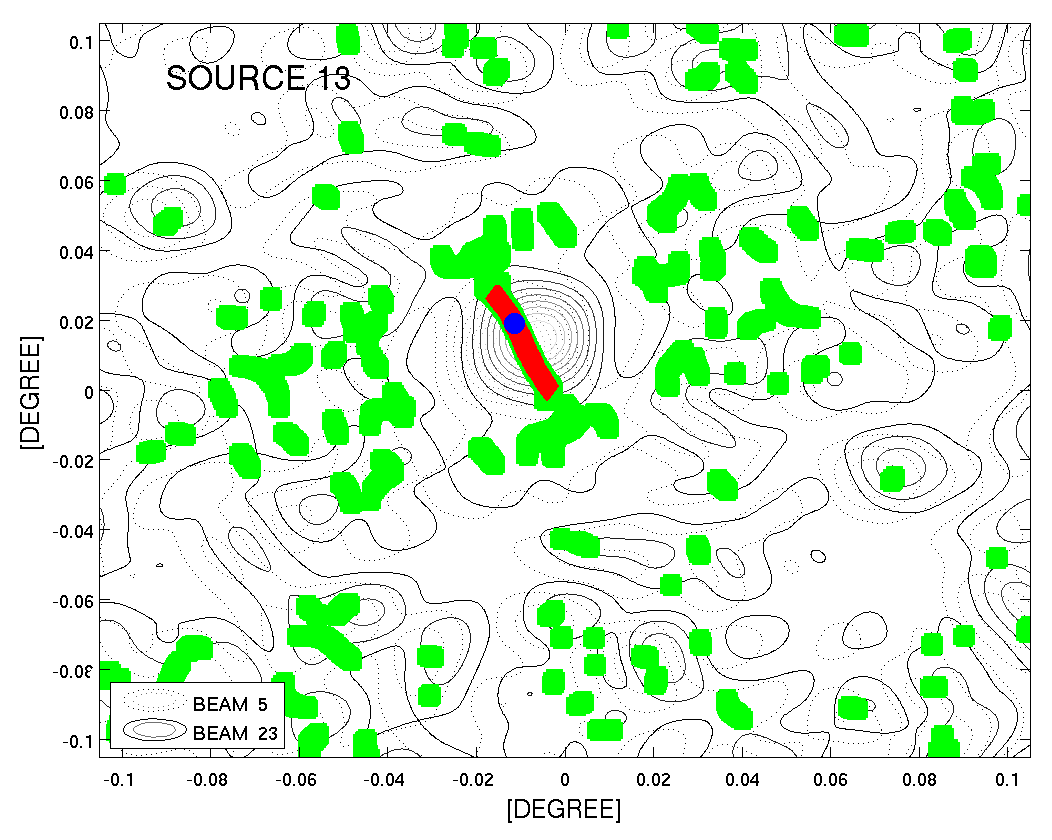
Figure 11: Detection examples, discussed in §4.2, with low and high positional uncertainty (left and right respectively) for the MUST array (top), the LOFAR array (middle) and MeerKAT array (bottom). (Green squares) values of $\mathfrak{s}_{1}/\mathfrak{s}_{2}$ and $(\mathfrak{a}_{2}-\mathfrak{a}_{1})$ from each TAB. The red diamonds regions where $\mathfrak{s}_{1}/\mathfrak{s}_{2}$ and $(\mathfrak{a}_{2}-\mathfrak{a}_{1})$ from all TABs overlap. The blue circles the true position of a source. Red regions in all cases include the true location of the source and so is obscured in the left panels in particular.

4.2.1 Detections with low positional uncertainty

The top left panel of Fig. 11 shows a detection of a source in six MUST TABs which Nyquist sample the FoV. Our estimated location of the source is completely consistent with the simulated position and the total area D to scan for a possible counterpart is only $0.04$ of the $\Omega_{HPBW_{L}}$. The middle right panel shows a detection in five LOFAR Superterp TABs which oversample the FoV. The total area D is $0.001$ of the $\Omega_{HPBW_{L}}$. The bottom right panel shows a detection in five MeerKAT core TABs which Nyquist sample the FoV, where the total area D is $0.003$ of the $\Omega_{HPBW_{L}}$. In all these cases the source was detected in at least five TABs and as a result the number of repeating values of $(\mathfrak{s}_{1}/\mathfrak{s}_{2})_{(i,\;j)}$ and $(\mathfrak{a}_{2}-\mathfrak{a}_{1})_{(i,\;j)}$ from all $(i,\;j)$ pairs of TABs is substantial (as indicated by the large areas of green). However, this illustrates why a detection in several TABs helps to accurately pin down its position as we are looking for values of $(\mathfrak{s}_{1}/\mathfrak{s}_{2})_{(i,\;j)}$ and $(\mathfrak{a}_{2}-\mathfrak{a}_{1})_{(i,\;j)}$ that are common to all TABs.

4.2.2 Detections with high positional uncertainty

The top right panel of Fig. 11 shows a detection of a source in two MUST TABs which oversample the FoV. ’Source 54’ is detected in a sidelobe of TAB 10 and the main beam of TAB 19. Unlike for the detections with low positional uncertainty, only two TABs are contributing $(\mathfrak{s}_{1}/\mathfrak{s}_{2})$ and $(\mathfrak{a}_{2}-\mathfrak{a}_{1})$ values. Thus, two possible locations are produced one of which is the real source position. However, the maximum area $\delta D_{Max}$ to scan for a counterpart is still only $0.01$ of the $\Omega_{HPBW_{L}}$. The middle left panel shows detection in three LOFAR TABs that Nyquist sample the FoV. Due to the complicated LOFAR beam pattern the values of $(\mathfrak{s}_{1}/\mathfrak{s}_{2})_{(i,\;j)}$ and $(\mathfrak{a}_{2}-\mathfrak{a}_{1})_{(i,\;j)}$ can be replicated as a result of low level variations in the beam pattern. However, from that example it is clear that even a three TAB detection can yield useful results as the maximum area $\delta D_{Max}$ to scan for a counterpart is only $0.002$ of the $\Omega_{HPBW_{L}}$. The bottom left panel shows a detection in two MeerKAT TABs which oversample the FoV. A two TAB only detection often produces large D. This is a common trend for all arrays. The area D for this example is equal to $1/2\Omega_{HPBW_{L}}$, but still it offers clues to the true source location and excludes a detection via a sidelobe.

4.3 Positional Accuracy Estimation

The results presented in Table 3 are summarised in Fig. 12. In the top panels we show the mean total area $\overline{D}$ covered by the estimated positions normalised to the TAB’s solid angle area $\Omega_{HPBW_{L}}$, where the error corresponds to one standard deviation from that mean for each m. Points without error bars indicate a single detection ($n=1$) for that m. The middle panels show the mean angular distance $\overline{\Delta\phi}$ between the estimated and the true source positions. The accuracy of our method can be best appreciated when these two sets of panels are examined together. For the MUST and MeerKAT arrays the positions of the majority of sources, 33 and 25 using Nyquist sampling and 30 and 38 using the oversampling method respectively, were estimated with a single position (m = 1). For LOFAR array, only 7 sources were estimated with a single position using Nyquist sampling. For LOFAR, the oversampling method provided higher accuracy, resulting in detection of 24 sources with a single position. As illustrated in the middle panels, a single estimated location on average guarantees a low angular separation $\delta\phi$ from the true source position. For example, for sources in group m = 1, the mean total area $\overline{D}$ for the MeerKAT array for both sampling methods has an area of $10\%$ of $\Omega_{HPBW_{L}}$ and the mean angular distance $\overline{\Delta\phi}$ is $8\%$ and $6\%$ of HPBW_L for the Nyquist sampling and oversampling methods respectively. Looking at the other end of the scale, the mean total area $\overline{D}$ for the sources in group m$\;>\;$5 is comparable to $\overline{D}$ for sources in group m = 1 for both sampling methods. However, the mean angular distance $\overline{\Delta\phi}$ of $66\%$ and the mean total area $\overline{D}$ of $86\%$ of $\Omega_{HPBW_{L}}$ suggests that the estimated locations include sidelobes as well.

The relative results of our method for finding a source location in a TAB, relative to the HPBW_L, favoured the MeerKAT core configuration. This is not unexpected since the MUST array is a small test array and the complicated beam pattern of the LOFAR Superterp would require a further development of this method to get the best out of the data. The oversampling of the FoV for the MeerKAT array gives the best results in terms of small mean total area $\overline{D}$ and the mean angular distance $\overline{\Delta\phi}$. All 43 sources detected in oversampled TABs have $\overline{D}$ less than $0.6$ of a HPBW_L area. For sources in group $m=1$, the locations of 13 sources were estimated within a single pixel. The mean angular distance for single-pixel sources is 0.3 arcsecond (0.006 of the MeerKAT HPBW_L) from the true source position.

4.3.1 Positional uncertainty for the MeerKAT array when the errors are independent

So far all simulations have assumed that the errors between TABs are highly correlated. In Table 5 we show for comparison the results for the MeerKAT array if we consider the errors on $(\mathfrak{s}_{1}/\mathfrak{s}_{2})_{(i,\;j)}$ and $(\mathfrak{a}_{2}-\mathfrak{a}_{1})_{(i,\;j)}$ to be independent. Using again an example for the Nyquist sampled method the $m=2$ group now contains only one source when the errors are independent since they are smaller when added quadratically. The maximum angular distance $\delta\phi_{max}$ for a detection in this group is 1.2 HPBW_L away from the true position. This is a substantial decrease from $\delta\phi_{max}=6.3$ (Table 4). In addition, the lower errors increased the number of source with a single estimated position. For example for the Nyquist sampled method the number of detections increased from 25 to 29 sources.

4.4 Intrinsic Spectral Index Recovery

A by-product of an accurate position estimation is recovery of the intrinsic spectral index $\alpha_{I}$. The last rows in Table 3 list the mean estimated intrinsic spectral index $\overline{\alpha_{I}}$ of a source and the standard deviation $\sigma$ from that mean from all estimated locations. Fig. 12 (bottom) shows the mean estimated intrinsic spectral index $\overline{\alpha_{I}}$ for combined sources in each m. For all arrays where only one small mean area $\overline{D}$ and small $\overline{\Delta\phi}$ were estimated, the recovered $\alpha_{I}$ is close to its assigned value of -2. Not unexpectedly, there is a clear correlation between the small angular offset $\delta\phi$ from the true source position and the accuracy of estimated $\alpha_{I}$. The more accurate the estimated position is the smaller the $\alpha_{I}$ error.

Table 4: Detection rates from a sample of 60 sources.

Array	Undersampling	Nyquist	Oversampling
MUST	14	40	40
LOFAR	3	48	55
MeerKAT	2	33	43

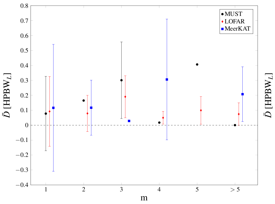
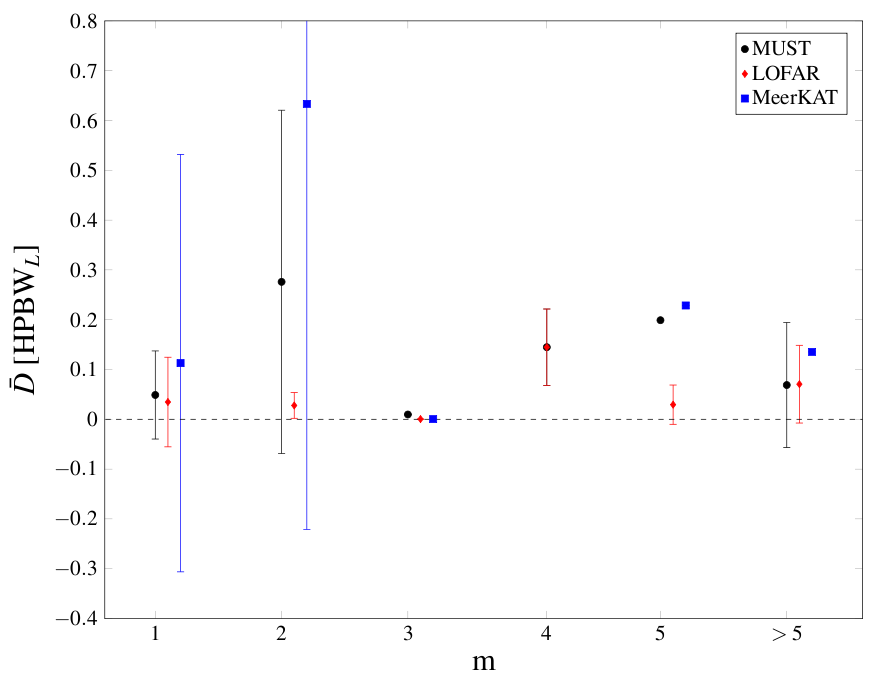
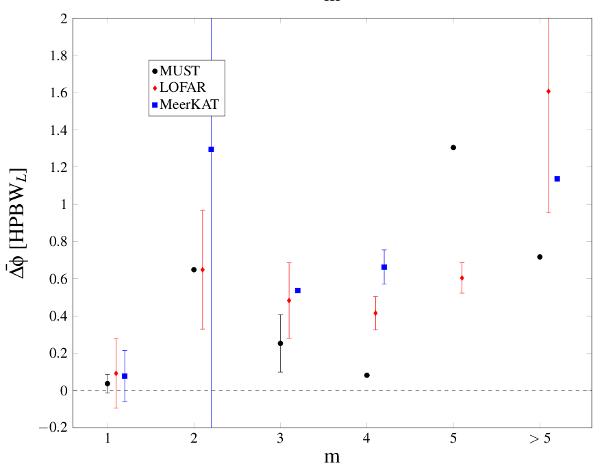
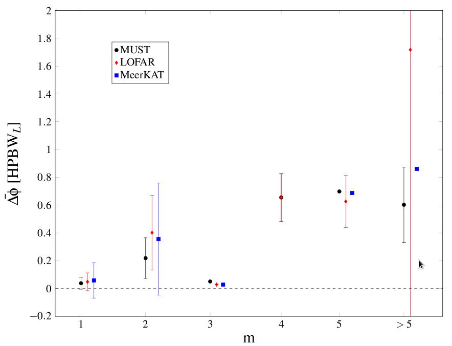
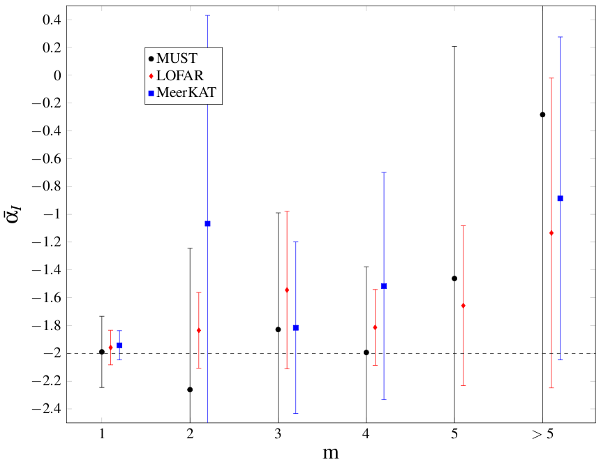
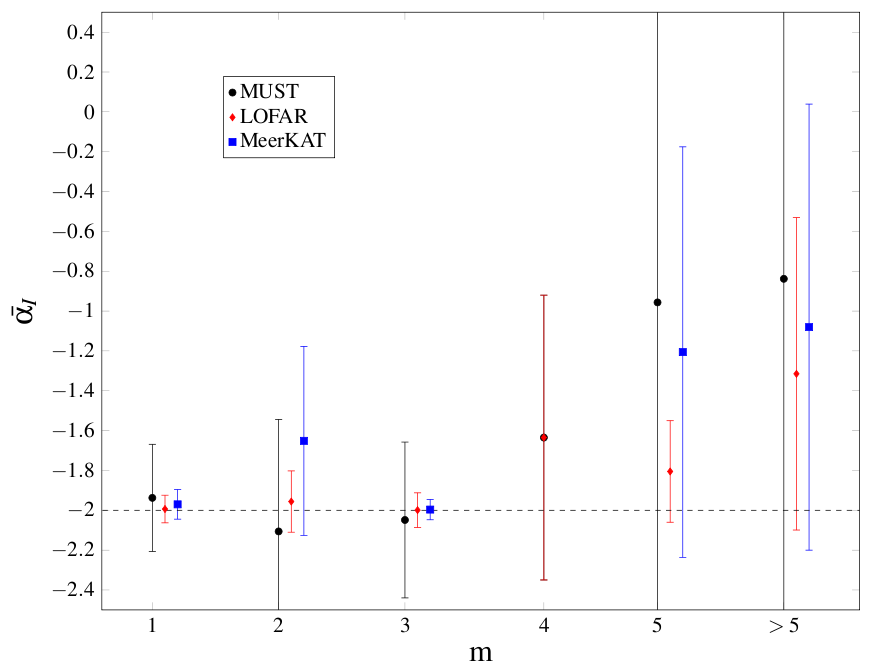
Figure 12: Summary of Table 3 for the Nyquist sampled (left) and oversampled (right) method. (top) The mean total area $\overline{D}$ covered by the estimated positions normalised to HPBW area in deg², where the error corresponds to one standard deviation from that mean for each m. (middle) The mean angular distance $\overline{\Delta\phi}$ between the estimated and the true source position. (bottom) The mean estimated intrinsic spectral index $\overline{\alpha_{I}}$ for combined sources in each m.

5 Discussion

In summary, we can broadly distinguish three basic levels in a hierarchy of positional accuracy within a TAB that can be achieved with the method presented here:

1. $\sim 1\times$HPBW accuracy;

2. $\sim 0.1\times$HPBW accuracy;

3. $\sim 0.01\times$HPBW accuracy or better.

For sources that fall into category (i) a detection can be constrained to a single or small group of TABs. The accuracies of (i) and (ii) may however be more than sufficient if the observations are conducted in parallel with follow-up telescopes with higher positional accuracy or in combination with a transient buffer. On the other hand the angular position of accuracy of (iii), depending on the maximum baseline, may already be sufficient to identify a host galaxy, or other related object without reference to other simultaneous observations.

It is clear that a high fractional bandwidth in the case of Nyquist sampling can prevent one or both of our conditions for detection to be realised. When the TABs Nyquist sample the FoV, the HPBW contours at $\nu_{H}$ are spaced further apart, as illustrated in Fig. 8, making our condition (b) difficult to meet. For such arrays oversampling of the FoV will clearly give higher detection rates. A beam pattern with high number of low level fluctuations, like LOFAR, can contribute to a higher detection rate, via detection in sidelobes, but also to a higher number of ”false positions”. On the other hand, a clean beam pattern, as produced by MeerKAT, results in lower detection rates but good location accuracy. For MeerKAT, the mean $\overline{\Delta\phi}$ for 38 out of 60 simulated sources, detected in the oversampled TABs, is less than $6\%$ of the HPBW_L, or less than 3 arcsecond from the true position. Thus, we were able to accurately estimate the source location for the majority of sources with a single simulated FRB observation.

While the oversampling of the FoV yields superior results for both the LOFAR and MeerKAT arrays there is a limit on how many TABs can be synthesised with a given back end. Some coverage of the FoV may therefore have to be sacrificed if a high location accuracy is desired and this has a trade-off in the survey speed. For example, say that a FoV is undersampled with N TABs, with N being the maximum number of TABs that can be synthesised. If we survey the same FoV with the Nyquist sampled TABs, the survey would take approximately 3.5 times longer. If we were to tile the FoV with the oversampled TABs, the survey would take approximately 4 times longer, for an array with $10\%$ fractional bandwidth. For an array with $20\%$ fractional bandwidth it would take 5 times longer.

For a real-time transient detection and localisation, the spatial information measured with sub-second resolution with a correlator interferometer requires high data rates. The current and the next generation radio telescopes typically provide both the beamforming mode and the correlation mode of observation. In that sense, the method we have described can provide high time resolution and highly useful, sometimes excellent, positional accuracy without increasing the computational burden of creating an image. Additionally, there is no significant delay between the detection and localisation. It is however still of high value to have a transient buffer available on all dishes in an array, because it will allow for greater sensitivity by making use of dishes outside of the core. In addition, the longer baselines will allow even further improvement determination of the source location. Being able to trigger and store the raw data from the dishes, and then use the position determined by our methods we can go back and form a higher sensitivity beamformed data set. This will consist of the raw complex data which can then be used for coherent dedispersion, in non-scattering-limited situations, to obtain the true width of the pulse. The raw complex data can also be used so that the full polarisation calibration, necessary to achieve the scientific goals mentioned in the introduction, can be achieved.

We stress that this paper describes only a proof-of-concept of the new method. There are practical issues still to be tackled before the method is ready for real world observations. In particular a thorough treatment of errors involving the effect of:

• the idealised model of the beam patterns;

• the shapes of the receiver bandpasses;

• the noise contributions of the receivers and sky;

will have to be addressed in future work. We also plan to investigate how other available scientific data, like the DM or polarisation, can be utilised. Furthermore, our simulations assumed a strict two frequency regime i.e. $\nu_{L}$ and $\nu_{H}$, but in practise the bandwidth can be split into many bands increasing the detection rates for high S/N transients and positively contributing to the accuracy of the estimated location. Another area of investigation would be to see whether simultaneously considering many frequency channels across the band is better than applying a known beam model before generating values at a smaller number of frequency channels. These steps, we believe, would also increase the usability of this method for arrays with complicated beam patterns, like the LOFAR Superterp. The implications of radio frequency interference (RFI) on the calculation of source flux density will be addressed in the next paper. However, it is unlikely that RFI will be spatially distinct compared to real sources so this method may provide further capability for discriminating against RFI.

6 Conclusions

We have presented a proof-of-concept analysis of a new non-imaging method for detecting and locating radio transient sources. It utilises the additional spectral and comparative spatial information from multiple TABs formed by an adding interferometer array to estimate a transient source location in almost real time. We have shown that this method can work in variety of interferometers but, not surprisingly, the method is most successful for arrays with good range of baselines, and hence clean array beam patterns. In this case transients with high S/N can be localised to small fractions of a HPBW of a TAB sufficient, in the case of MeerKAT, to localise a source to arcsecond accuracy. Even less certain positions can still be very useful if there is a parallel transient search in the same field at a different wavelength. In a future paper we will address a range of practical issues which will need to be taken into account in an operational implementation of this scheme.

We thank Jayanta Roy for useful discussions and for the help in improving the clarity of this paper. We would like to thank the referee for providing comments which serve to improve and clarify the paper. We want to extend our appreciation for taking the time to comment on our manuscript to the editor.

Table 5: Comparison of the accuracy of the Nyquist sampled and oversampled methods for determining the positions and the intrinsic spectral index for the MeerKAT core for the case when the errors are independent. Here m is the number of locations estimated per detected source. n is the number of sources detected at the number of positions shown. $\overline{B}$ is the mean number of TABs per source. Below we list the minimum ($\delta D_{Min}$), maximum ($\delta D_{Max}$) and mean ($\overline{D}$) value of the total area D covered by the overlapping values of $\mathfrak{s}_{1}/\mathfrak{s}_{2}$ and $(\mathfrak{a}_{2}-\mathfrak{a}_{1})$, normalised to the $\Omega_{HPBW_{L}}$ area in deg². The total area D represents the area that would need to be sampled in follow up, or archival, observations to be sure that the actual position of the source was observed. We also list the minimum ($\delta\phi_{Min}$), maximum ($\delta\phi_{Max}$) and mean ($\overline{\Delta\phi}$) value of the total angular distances $\Delta\phi$ between the true and the estimated source position, normalised to the HPBW_L. $\overline{\alpha_{I}}$ is the mean estimated intrinsic spectral index of all sources from group m where $\sigma$ is the standard deviation from that mean.

		MeerKAT
Parameter		Nyquist sampling						Oversampling
m		1	2	3	4	5	¿5		1	2	3	4	5	¿5
n		29	1	1	-	-	2		39	2	-	-	1	1
$\overline{B}$		4	2	2	-	-	2		5	4	-	-	2	2
D
	$\delta D_{Min}$	0.0004	0.0008	0.006	-	-	0.0004		0.0004	0.0004	-	-	0.0008	0.0004
	$\delta D_{Max}$	2	0.5	2.1	-	-	1.8		1.9	2.3	-	-	0.7	0.8
	$\overline{D}$	0.09	0.27	0.70	-	-	0.19		0.11	0.58	-	-	0.16	0.13
$\delta\phi$
	$\delta\phi_{Min}$	0.001	0.002	0.008	-	-	0.007		0.001	0.006	-	-	0.008	0.002
	$\delta\phi_{Max}$	1.3	1.2	6.2	-	-	11		1.4	6.1	-	-	11	11
	$\overline{\Delta\phi}$	0.06	0.59	0.72	-	-	0.85		0.05	0.30	-	-	0.68	0.88
$\alpha_{I}$
	$\overline{\alpha_{I}}$	-2.1	-1.6	-1.3	-	-	-1.1		-2.1	-1.7	-	-	-1.2	-1.1
	$\sigma$	0.1	0.8	0.8	-	-	1.1		0.1	0.4	-	-	1.1	1.1

References

- Bannister & Cornwell (2011) Bannister K. W., Cornwell T. J., 2011, ApJS, 196, 16
- Bannister et al. (2012) Bannister K. W., Murphy T., Gaensler B. M., Reynolds J. E., 2012, The Astrophysical Journal, 757, 38
- Booth et al. (2009) Booth R. S., de Blok W. J. G., Jonas J. L., Fanaroff B., 2009, ArXiv e-prints
- Burke-Spolaor et al. (2011) Burke-Spolaor S., Bailes M., Ekers R., Macquart J.-P., Crawford F., III, 2011, ApJ, 727, 18
- Burke-Spolaor & Bannister (2014) Burke-Spolaor S., Bannister K. W., 2014, ApJ, 792, 19
- Cen & Ostriker (1999) Cen R., Ostriker J. P., 1999, ApJ, 514, 1
- Chippendale et al. (2010) Chippendale A. P., O’Sullivan J., Reynolds J., Gough R., Hayman D., Hay S., 2010, in Phased Array Systems and Technology (ARRAY), 2010 IEEE International Symposium on, pp.648-652, 12-15 Oct. 2010, p. 648
- Cordes et al. (2006) Cordes J. M. et al., 2006, ApJ, 637, 446
- Cordes & Lazio (2002) Cordes J. M., Lazio T. J. W., 2002, ArXiv Astrophysics e-prints
- Deng & Zhang (2014) Deng W., Zhang B., 2014, ApJ, 783, L35
- Gao et al. (2014) Gao H., Li Z., Zhang B., 2014, ApJ, 788, 189
- Haslam et al. (1982) Haslam C. G. T., Stoffel H., Salter C. J., Wilson W. E., 1982, A&AS, 47, 1
- Hassall et al. (2013) Hassall T. E., Keane E. F., Fender R. P., 2013, MNRAS, 436, 371
- Keane et al. (2012) Keane E. F., Stappers B. W., Kramer M., Lyne A. G., 2012, MNRAS, 425, L71
- Kouwenhoven & Voûte (2001) Kouwenhoven M. L. A., Voûte J. L. L., 2001, A&A, 378, 700
- Law & Bower (2014) Law C. J., Bower G. C., 2014, in Exascale Radio Astronomy, p. 20303
- Law et al. (2014) Law C. J. et al., 2014, ArXiv e-prints
- Law et al. (2011) Law C. J., Jones G., Backer D. C., Barott W. C., Bower G. C., Gutierrez-Kraybill C., Williams P. K. G., Werthimer D., 2011, ApJ, 742, 12
- Lorimer et al. (2007) Lorimer D. R., Bailes M., McLaughlin M. A., Narkevic D. J., Crawford F., 2007, Science, 318, 777
- Lorimer et al. (2006) Lorimer D. R. et al., 2006, MNRAS, 372, 777
- Lorimer et al. (2013) Lorimer D. R., Karastergiou A., McLaughlin M. A., Johnston S., 2013, ArXiv e-prints
- Macquart & Koay (2013) Macquart J.-P., Koay J. Y., 2013, ApJ, 776, 125
- Manchester et al. (2006) Manchester R. N., Fan G., Lyne A. G., Kaspi V. M., Crawford F., 2006, ApJ, 649, 235
- Manchester et al. (2001) Manchester R. N. et al., 2001, MNRAS, 328, 17
- McQuinn (2014) McQuinn M., 2014, ApJ, 780, L33
- Nan et al. (2011) Nan R. et al., 2011, International Journal of Modern Physics D, 20, 989
- Oosterloo et al. (2010) Oosterloo T., Verheijen M., van Cappellen W., 2010, in ISKAF2010 Science Meeting
- Palaniswamy et al. (2014) Palaniswamy D., Wayth R. B., Trott C. M., McCallum J. N., Tingay S. J., Reynolds C., 2014, The Astrophysical Journal, 790, 63
- Petroff et al. (2014) Petroff E. et al., 2014, ArXiv e-prints
- Ravi et al. (2014) Ravi V., Shannon R. M., Jameson A., 2014, ArXiv e-prints
- Reich & Reich (1988) Reich P., Reich W., 1988, A&A, 196, 211
- Spitler et al. (2014) Spitler L. G. et al., 2014, ArXiv e-prints
- Thornton et al. (2013) Thornton D. et al., 2013, Science, 341, 53
- van Haarlem et al. (2013) van Haarlem M. P. et al., 2013, A&A, 556, A2
- Zhou et al. (2014) Zhou B., Li X., Wang T., Fan Y.-Z., Wei D.-M., 2014, Phys. Rev. D, 89, 107303