Abstract

We study the process $e^{-}e^{+}\to\gamma H$, where $H$ represents $H_{SM}$, $h^{0}$ or $H^{0}$. This process occurs at the one loop level in the standard model (SM) or in the minimal supersymmetric standard model (MSSM). We establish supersimple (sim) high energy expressions for all helicity amplitudes of this process, and we identify their level of accuracy for describing the various polarized and unpolarized observables, and for distinguishing SM from MSSM or another beyond the standard model (BSM). We pay a special attention to transverse $e^{\mp}$ polarization and azimuthal dependencies induced by the imaginary parts of the amplitudes, which are relatively important in this process.

PACS numbers: 12.15.-y, 12.60.-i, 13.66.Fg

1 Introduction

After the discovery [1] of the Higgs boson [2], detailed experimental and theoretical studies are necessary for checking its properties and dynamics [3, 4]. Within this aim, we have recently studied the process $e^{-}e^{+}\to ZH$ [5], where $H$ represents $(H_{SM},h^{0},H^{0})$. This process occurs at the one loop level in the standard model (SM) or the minimal supersymmetric standard model (MSSM), and is observable at future linear colliders [6, 7], and also at future circular colliders; see [8]. We have analyzed the contents of its amplitudes in SM and MSSM, their consequences for the various observables, and we have established simple expressions which approximate them at high energy.

In the present paper we consider the process $e^{-}e^{+}\to\gamma H$ which, contrarily to $e^{-}e^{+}\to ZH$, has no Born term and should be relatively more affected by anomalous effects. The basic amplitudes are arising at electroweak one loop order [9, 10]. These contributions contain specific SM or MSSM parts that we discuss. Due to the absence of real Born terms, the imaginary parts of the one loop amplitudes play here an important role and we look for the consequences of this feature.

We start from the complete computation of these one loop amplitudes in SM and MSSM, in order to dispose of the exact expressions in terms of Passarino-Veltman (PV) functions [11]. From their expansions at high energy [12], we then establish simple approximate expressions called supersimple (sim), as in the other similar recent studies on $(gg\to\gamma\gamma,~{}\gamma Z,~{}ZZ,W^{-}W^{+})$, $ug\to dW^{+}$ and $(e^{-}e^{+}\to t\bar{t},~{}W^{-}W^{+},~{}ZH)$, [13, 14, 15, 5]. As before, we expect that these simple expressions will be useful for making quick estimates of the amplitudes and meaningful comparisons with experimental results.

In addition, during the analysis of $e^{-}e^{+}\to ZH$ [5], we have found that some observables are especially sensitive to the underlying dynamics; i.e. SM, MSSM or another BSM. Our aim is therefore to check whether this is also the case for $e^{-}e^{+}\to\gamma H$. Particularly because $e^{-}e^{+}\to\gamma H$ is determined by the helicity violating (HV) amplitudes at high energies, in contrast to the processes aforementioned in the preceding paragraph, which are dominated by their helicity conserving (HC) amplitudes [16, 17]. As we show in the Appendix, one consequence of this is that the augmented Sudakov-type quadratic logarithms in $e^{-}e^{+}\to\gamma H$ do not retain the universal structure observed in $(gg\to\gamma\gamma,~{}\gamma Z,~{}ZZ,W^{-}W^{+})$, $ug\to dW^{+}$, $(e^{-}e^{+}\to t\bar{t},~{}W^{-}W^{+},~{}ZH)$, [13, 14, 15, 5].

This way, we have calculated various polarized and unpolarized cross sections and asymmetries, and studied their sensitivity to the underlying dynamics. In addition, we also consider the possibility of transversally polarized $e^{-}e^{+}$ beams, where the presence of imaginary parts in the $e^{-}e^{+}\to\gamma H$ amplitudes leads to a particular azimuthal $\sin 2\phi$ dependence, supplying further dynamical tests.

The contents of the paper are the following: In Sect.2 we give the notation for the kinematics and the helicity amplitudes. In Sect.3 we present the electroweak (EW) one loop contributions and establish their supersimple expressions, explicitly written in the Appendix. Sect.4 is devoted to the description of other BSM effects in terms of effective couplings. The various observables are defined in Sect.5. The numerical analysis is presented in Sect.6 with many illustrations, while the conclusions are given in Sect.7.

2 Kinematics and helicity amplitudes

The kinematics of the process

$$e^{-}_{\lambda}(l)~{}e^{+}_{\lambda^{\prime}}(l^{\prime})\to\gamma_{\tau}(p)~{}H(p^{\prime})~{}~{},$$ (1)

is defined in terms of the helicities $(\lambda,\lambda^{\prime})$ of the incoming $(e^{-},e^{+})$ beams, and the helicity $\tau$ of the outgoing $\gamma$, whose polarization vector is $\epsilon$. The momenta of the various incoming and outgoing particles are $(l,l^{\prime},p,p^{\prime})$, and we also use

$$s=(l+l^{\prime})^{2}=(p+p^{\prime})^{2}~{}~{},~{}~{}t=(l-p)^{2}=(l^{\prime}-p^{\prime})^{2},~{}~{}u=(l-p^{\prime})^{2}=(l^{\prime}-p)^{2}~{}~{},~{}~{}$$

$$p_{\gamma}=E_{\gamma}={s-m^{2}_{H}\over 2\sqrt{s}}=\beta_{\gamma}{s\over 2}~{}~{},$$ (2)

where $p_{\gamma}=E_{\gamma}=p$ denote the equal values of the three-momentum and energy of the outgoing photon, and $\theta$ is the angle between the direction of the incoming $e^{-}$ and the outgoing $\gamma$.

The general invariant amplitude is written as

$$A=\sum_{i}N_{i=1,3,4}(s,t)I_{i}+N^{\prime}_{1}(s,t)J_{1}$$ (3)

using the forms

$$I_{1}=\bar{v}(e^{+}_{\lambda^{\prime}})~{}\hbox to0.0pt{/\hss}\epsilon~{}u(e^{-}_{\lambda})~{}~{},~{}~{}I_{3}=\bar{v}(e^{+}_{\lambda^{\prime}})~{}\epsilon\cdot l^{\prime}\hbox to0.0pt{/\hss}p~{}~{}u(e^{-}_{\lambda})~{}~{},~{}~{}I_{4}=\bar{v}(e^{+}_{\lambda^{\prime}})~{}\epsilon\cdot l\hbox to0.0pt{/\hss}p~{}u(e^{-}_{\lambda})~{}~{},$$ (4)

$$J_{1}=-i\bar{v}(e^{+}_{\lambda^{\prime}})\epsilon^{\mu\nu\rho\sigma}\gamma_{\mu}\epsilon_{\nu}p^{\prime}_{\rho}p_{\sigma}u(e^{-}_{\lambda})~{}~{},$$ (5)

already used in [5]. Note that the $J_{1}$ form only appears in the case of CP-violating couplings; see Sect.4.

The scalar functions $N_{i=1,3,4}(s,t),N^{\prime}_{1}(s,t)$ are obtained by computation of specific diagrams. One then gets the corresponding helicity amplitudes $F_{\lambda,\tau}(s,\theta)$ by usual expansion of the Dirac spinors appearing in the forms (4, 5), using the standard Jacob-Wick conventions [18]; note that $\tau=\pm 1$ and that

$$\lambda=-\lambda^{\prime}=\mp{1\over 2}~{}~{}~{},$$ (6)

when one neglects the electron mass. The notation $(\lambda=L,R)$ for these two cases of $e^{\mp}$ helicity is also used. This way one then gets

$$I_{1}\to\delta_{\lambda,L}\sqrt{s\over 2}(\tau\cos\theta-1)-\delta_{\lambda,R}\sqrt{s\over 2}(\tau\cos\theta+1))~{},~{}$$

$$I_{3}=-I_{4}\to(\delta_{\lambda,R}-\delta_{\lambda,L}){ps\over 2\sqrt{2}}\tau\sin^{2}\theta~{},~{}$$

$$J_{1}\to 2\lambda{ps\over\sqrt{2}}(\cos\theta+2\lambda\tau)~{}.$$ (7)

Due to (6), the helicity amplitudes $F_{\lambda,\tau}(s,\theta)$ violate the high energy Helicity Conservation (HCns) rule [16, 17] which requires

$$\lambda+\lambda^{\prime}=\tau~{}~{}.$$ (8)

They are thus called helicity violating (HV) amplitudes, and they are indeed vanishing at high energy in MSSM or SM.

When CP is conserved, the additional constraint

$$F_{\lambda,\tau}(s,\theta)=F_{\lambda,-\tau}(s,\pi-\theta)~{}~{},$$ (9)

also holds, reducing the independent amplitudes to only two.

3 The one loop EW corrections and their supersimple (sim) expressions in SM and MSSM.

The one-loop amplitudes of the process $e^{-}e^{+}\to\gamma H$ consist of a reduced set of the diagrams appearing in the $ZH$ case (replacing of course the $Z$ couplings by the $\gamma$ ones). Having no Born terms, there is no self-energy corrections nor renormalization counter terms. There are also no $s$-channel initial triangles, because of the absence of any $H\gamma\gamma,HZ\gamma$ couplings.

Thus, the one loop diagrams in the SM case consist only of final triangles in $s$-channel, up and down triangles in $t$ and $u$ channels, direct, crossed and twisted boxes, and specific diagrams involving 4-leg bosonic couplings; see [9, 10, 19]. In the MSSM case we also have corresponding diagrams involving supersymmetric partners like sleptons, squarks, charginos, neutralinos and additional Higgses. As in [5], we always restrict to CP-conserving SM or MSSM couplings, so that (9) is satisfied.

We have computed all these contributions in terms of PV functions [11]. This gives the exact basic contributions. We then compute their high energy expansions using the forms in [12]. The results thus obtained, called sim results, are given in the Appendix. As already mentioned in Sect.2, the $e^{-}e^{+}\to\gamma H$ amplitudes are of helicity violating (HV) type [16, 17]. Because of this, for SM or MSSM, they are suppressed at high energies like $M/\sqrt{s}$, tempered by terms involving single and double logarithms.

4 Other BSM effects

Apart from MSSM, another possibility of BSM physics is by inserting anomalous couplings to the SM gauge and Higgs bosons. There are various types of such models. One consequence of them for the process $e^{-}e^{+}\to\gamma H$ is the appearance of Born terms with intermediate $\gamma,Z$ exchanges and final $\gamma\gamma H$ and $\gamma ZH$ couplings. Our aim is just to see how the generated amplitudes and observables can differ from the one loop SM or MSSM predictions, and at what level of accuracy the sim expressions are adequate for that purpose.

As an example of such a BSM model we consider the description [20] of the anomalous couplings of the gauge and SM Higgs field given by the 2 CP-conserving operators $O_{UW}$, $O_{UB}$ and the 2 CP-violating ones $\bar{O}_{UW}$, $\bar{O}_{UB}$,

$${\cal O}_{UW}=\frac{1}{v^{2}}\left(\Phi^{\dagger}\Phi-\frac{v^{2}}{2}\right)\overrightarrow{W}^{\mu\nu}\overrightarrow{W}_{\mu\nu}~{}~{},~{}~{}{\cal O}_{UB}=\frac{4}{v^{2}}\left(\Phi^{\dagger}\Phi-\frac{v^{2}}{2}\right)B^{\mu\nu}B_{\mu\nu}~{}~{},$$

$${\bar{\cal O}}_{UW}=\frac{1}{v^{2}}(\Phi^{\dagger}\Phi)\overrightarrow{W}^{\mu\nu}\widetilde{\overrightarrow{W}}_{\mu\nu}~{}~{},~{}~{}{\bar{\cal O}}_{UB}=\frac{4}{v^{2}}(\Phi^{\dagger}\Phi)B^{\mu\nu}\widetilde{B}_{\mu\nu}~{}~{},$$ (10)

where $\Phi$ is the SM Higgs doublet field, with the vacuum expectation value of its neutral component satisfying $<\phi^{0}>\sqrt{2}\equiv v=(G_{F}\sqrt{2})^{-1}$ at tree level. Inserting the operators (10) in the SM lagrangian induces a BSM term given by

$$\delta{\cal L}_{BSM}=d_{UW}{\cal O}_{UW}+d_{UB}{\cal O}_{UB}+\bar{d}_{UW}{\bar{\cal O}}_{UW}+\bar{d}_{UB}{\bar{\cal O}}_{UB}~{}~{},$$ (11)

which in turn creates the anomalous $\gamma\gamma H_{SM}$ and $\gamma ZH_{SM}$ couplings

$$d_{\gamma Z}=s_{W}c_{W}(d_{UW}-d_{UB}) d_{\gamma\gamma}=(d_{UB}s^{2}_{W}+d_{UW})c^{2}_{B}~{}~{},$$ ,

$$\bar{d}_{\gamma Z}=s_{W}c_{W}(\bar{d}_{UW}-\bar{d}_{UB}) \bar{d}_{\gamma\gamma}=(\bar{d}_{UB}s^{2}_{W}+\bar{d}_{UW})c^{2}_{B}~{}~{}.$$ , (12)

Denoting $V=\gamma,Z$ and using

$$g^{\gamma}_{eL}=g^{\gamma}_{eR}=q_{e}=-1~{}~{},~{}~{}g^{Z}_{eL}={-1+2s^{2}_{W}\over 2s_{W}c_{W}}~{}~{},~{}~{}g^{Z}_{eR}={s_{W}\over c_{W}},~{}~{}$$ (13)

the induced (Born type with $V$ exchange) anomalous contribution to the invariant amplitude becomes

$$A=-~{}\sum_{V}{e^{2}\over(s-m^{2}_{V})}~{}[g^{V}_{1}~{}I_{1}+g^{\prime V}_{1}~{}J_{1}]~{}[g^{V}_{eL}P_{L}+g^{V}_{eR}P_{R}]~{}~{},$$ (14)

where the CP-conserving part appears with the $I_{1}$ form defined in (4) and the couplings

$$g^{\gamma}_{1}={2E_{\gamma}\sqrt{s}\over m_{Z}s_{W}c_{W}}d_{\gamma\gamma} g^{Z}_{1}=~{}{2E_{\gamma}\sqrt{s}\over m_{Z}s_{W}c_{W}}d_{\gamma Z}~{}~{},$$ , (15)

while the CP violating part is given by $J_{1}$ of (5) and the couplings

$$g^{\prime\gamma}_{1}={2\over m_{Z}s_{W}c_{W}}\bar{d}_{\gamma\gamma} g^{\prime Z}_{1}=~{}{2\over m_{Z}s_{W}c_{W}}\bar{d}_{\gamma Z}~{}~{}.$$ , (16)

In the illustrations presented in Sect. 6, we choose the CP conserving and the CP-violating BSM couplings in (11), so that the BSM amplitudes are comparable to the 1 loop SM results, in the high energy domain ($\lesssim 5$ TeV) considered here. More explicitly, we then show separately two cases with non-vanishing couplings, respectively called

$$(d_{UW}=0.00017~{},~{}\bar{d}_{UW}=0.0001) \Rightarrow {\rm W~{}eff}~{}~{},$$ (17)

$$(d_{UB}=0.00017~{},~{}\bar{d}_{UB}=0.0001) \Rightarrow {\rm B~{}eff}~{}~{}.$$ (18)

Note that the (HCns) rule [16, 17] does not apply to such anomalous non renormalizable contributions. Because of this, such BSM amplitudes are not suppressed at high energy.

5 Observables and amplitude analysis

Contrary to the $ZH$ case, where real amplitude contributions coming from the Born terms dominate, in the $\gamma H$ case the four independent helicity amplitudes are complex and one would need 8 independent observables in order to make a complete analysis. This would require longitudinal and transverse initial $e^{\mp}$, as well as final $\gamma$ polarizations; these last ones being probably very difficult to measure.

When CP is conserved, only two independent complex helicity amplitudes occur, and one would need only 4 observables (at a given energy and all angles) in order to make the amplitude analysis.

In presenting these observables we use the same notation as in [5]. A lower index like $L$ or $R$ refers to the initial $e^{-}$ polarization and corresponds to $\lambda=-{1\over 2}$ or $\lambda=+{1\over 2}$ respectively. The final photon polarization is denoted by an index $\gamma_{\tau}$ for $\tau=\pm 1$. Quantities like $\sigma(\lambda,\tau)$ can then be also denoted as $\sigma^{\gamma_{\tau}}_{L,R}$; see also immediately after (6).

The differential unpolarized cross sections and the corresponding integrated ones over all $\theta$ angles are respectively given by

$${d\sigma\over d\cos\theta}={\beta_{\gamma}\over 128\pi s}\sum_{\lambda\tau}|F_{\lambda\tau}(\theta)|^{2}~{}~{},$$ (19)

and

$$\sigma=\int^{1}_{-1}d\cos\theta{d\sigma\over d\cos\theta}~{}~{},$$ (20)

where $\beta_{\gamma}$ is defined in (2) and the summations apply over $\lambda=\pm{1\over 2}$ and $\tau=\pm 1$.

Correspondingly, unpolarized (or polarized with the adequate index) cross sections integrated over the forward (with respect to the $e^{-}$-beam) or the backward region, are respectively denoted as $\sigma_{F}$ and $\sigma_{B}$.

Polarization asymmetries
These contain initial $e^{-}_{L}$-$e^{-}_{R}$ asymmetries, with the $\gamma$ helicity being either not observed, or chosen to have specific value $\tau=\pm 1$

$$A_{LR}={\sigma_{L}-\sigma_{R}\over\sigma_{L}+\sigma_{R}}~{}~{},$$ (21)

$$A_{LR}(\tau)={\sigma_{L}(\tau)-\sigma_{R}(\tau)\over\sigma_{L}(\tau)+\sigma_{R}(\tau)}~{}~{};~{}~{}$$ (22)

or asymmetries defined with respect the final $\gamma$ polarization, with the $e^{\mp}$ beams selected to be either unpolarized, or the electrons being either purely $e^{-}_{L}$ or purely $e^{-}_{R}$

$$A^{{\rm pol}~{}\gamma}={\sigma(\tau=-)-\sigma(\tau=+)\over\sigma(\tau=-)+\sigma^{(}\tau=+)}\equiv{\sigma^{\gamma_{-}}-\sigma^{\gamma_{+}}\over\sigma^{\gamma_{-}}+\sigma^{\gamma_{+}}}~{}~{},$$ (23)

$$A^{{\rm pol}~{}\gamma}(\lambda)={\sigma(\lambda,\tau=-)-\sigma(\lambda,\tau=+)\over\sigma(\lambda,\tau=-)+\sigma(\lambda,\tau=+)}\equiv{\sigma^{\gamma_{-}}_{\lambda}-\sigma^{\gamma_{+}}_{\lambda}\over\sigma^{\gamma_{-}}_{\lambda}+\sigma^{\gamma_{+}}_{\lambda}}~{}~{}.$$ (24)

Forward-backward asymmetries
In the unpolarized beam case, when the final photon polarization is not looked at, these are defined as

$$A_{FB}={\sigma_{F}-\sigma_{B}\over\sigma_{F}+\sigma_{B}}~{}~{};$$ (25)

while for any definite $e^{-}$ and photon helicity they are defined as

$$A_{FB}(\lambda,\tau)={\sigma_{F}(\lambda,\tau)-\sigma_{B}(\lambda,\tau)\over\sigma_{F}(\lambda,\tau)+\sigma_{B}(\lambda,\tau)}~{}~{}.$$ (26)

Combining (24, 26), one obtains a peculiar forward-backward asymmetry of the above $\gamma$ transverse polarization asymmetry,

$$A^{{\rm pol}~{}\gamma}_{FB}={(\sigma^{\gamma_{-}}-\sigma^{\gamma_{+}})_{F}-(\sigma^{\gamma_{-}}-\sigma^{\gamma_{+}})_{B}\over(\sigma^{\gamma_{-}}+\sigma^{\gamma_{+}})_{F}+(\sigma^{\gamma_{-}}+\sigma^{\gamma_{+}})_{B}}~{}~{},$$ (27)

which may be defined for unpolarized $e^{\mp}$ beams, as well as separately for $L$ or $R$ electron beams. It turns out to be non vanishing in all these three cases.

CP conservation
When CP is conserved, one gets from (9)

$$A_{FB}(\lambda,-\tau)=-A_{FB}(\lambda,\tau)~{}~{},$$ (28)

which remains true also for unpolarized $e^{\mp}$-beams, where one sums over $\lambda=L,R$ obtaining

$$A_{FB}(-\tau)=-A_{FB}(\tau)~{}~{}\Rightarrow~{}~{}A_{FB}(\gamma_{+})=-A_{FB}(\gamma_{-})~{}~{}.$$ (29)

If one sums over all final $\gamma$ polarization in (29), then one obtains $A_{FB}=0$.

Another consequence of CP conservation concerns the Left-Right asymmetries in the forward and backward directions

$$A^{F}_{LR}(\tau)=A^{B}_{LR}(-\tau)\Rightarrow A^{F}_{LR}(\gamma_{-})=A^{B}_{LR}(\gamma_{+})~{}~{};$$ (30)

compare (22).

We also note that CP conservation implies

$$A_{F}^{{\rm pol}~{}\gamma}(\lambda)=-A_{B}^{{\rm pol}~{}\gamma}(\lambda)~{}~{},$$ (31)

for both $\lambda=L,R$ cases, such that the totally integrated $A^{{\rm pol}~{}\gamma}(\lambda)$ vanishes; compare (27).

In the next section we illustrate the above properties for CP conserving one loop corrections to SM or MSSM models; as well as for the effective, possibly CP violating Higgs couplings in the BSM case (11). It turns out that some of the above asymmetries are particularly sensitive to the dynamical details, and may be very useful for disentangling SM from MSSM or BSM corrections.

Transverse $e^{\pm}$ polarization
We next turn to the possibility of $e^{-}e^{+}$ collisions with transversally polarized beams. It has been known since a long time, that this can reveal in a clear way the presence of various types of BSM effects; see e.g. [21, 22, 23]. In our case, this is particularly motivated by the presence of a relatively important imaginary part in the $e^{-}e^{+}\to\gamma H$ amplitudes, which may produce an important $\sin 2\phi$ azimuthal dependence in the transition probability. Restricting to (6), we then obtain

$$R=R_{0}+2P_{T}P^{\prime}_{T}[\cos 2\phi R_{\cos 2\phi}+\sin 2\phi R_{\sin 2\phi}]~{}~{},$$ (32)

with the unpolarized part being

$$R_{0}=|F_{--}|^{2}+|F_{-+}|^{2}+|F_{+-}|^{2}+|F_{++}|^{2}~{}~{},$$ (33)

$(P_{T},P^{\prime}_{T}$) being the $e^{\mp}$ degrees of transverse polarization, and the two azimuthal dependent terms being

$$R_{\sin 2\phi} = {\rm Im}F_{--}{\rm Re}F_{+-}-{\rm Re}F_{--}{\rm Im}F_{+-}+{\rm Im}F_{-+}{\rm Re}F_{++}-{\rm Re}F_{-+}{\rm Im}F_{++}~{},$$ (34)

$$R_{\cos 2\phi} = {\rm Re}F_{--}{\rm Re}F_{+-}+{\rm Im}F_{--}{\rm Im}F_{+-}+{\rm Re}F_{-+}{\rm Re}F_{++}+{\rm Im}F_{-+}{\rm Im}F_{++}~{}.$$ (35)

Note that only the $\sin 2\phi$-term is proportional to the imaginary parts of the amplitudes, while the $\cos 2\phi$ term is non vanishing even when all amplitudes are purely real.

These $R_{0}$, $R_{\sin 2\phi}$, $R_{\cos 2\phi}$ terms can be extracted from the observed $R$-form in (32) by integrating the complete azimuthal distribution over the angular domains

$$\Big{[}0,2\pi\Big{]}~{},~{}$$

$${1\over 4}\Big{[}\Big{(}0,{\pi\over 2}\Big{)}-\Big{(}{\pi\over 2},\pi\Big{)}+\Big{(}\pi,{3\pi\over 2}\Big{)}-\Big{(}{3\pi\over 2},\pi\Big{)}\Big{]}~{},~{}$$

$${1\over 2}\Big{[}\Big{(}0,{\pi\over 4}\Big{)}-\Big{(}0,{3\pi\over 4}\Big{)}+\Big{(}\pi,{5\pi\over 4}\Big{)}-\Big{(}\pi,{7\pi\over 4}\Big{)}\Big{]}~{}.$$ (36)

Note that in case of CP conservation, the validity of (9) makes the three forms $R_{0}$, $R_{\sin 2\phi}$, $R_{\cos 2\phi}$, Forward-Backward symmetric.

In the illustrations of these transverse terms, we present the ratios of the polarized terms to the unpolarized one:

$$T_{\sin 2\phi}={2R_{\sin 2\phi}\over R_{0}}~{}~{},~{}~{}T_{\cos 2\phi}={2R_{\cos 2\phi}\over R_{0}}~{}~{}.$$ (37)

6 Numerical analysis

For the MSSM illustrations, we use the S1 benchmark of [24], where the EW scale values of the various parameters (with masses in TeV) are

$$\mu=0.4~{},~{}m_{A^{0}}=0.5~{},~{}M_{1}=0.25~{},~{}M_{2}=0.5~{},~{}M_{3}=2~{},$$

$$\tan\beta=20~{},~{}m_{\tilde{q}}=2~{},~{}m_{\tilde{l}}=A_{\tau}=0.5~{},~{}A_{t}=A_{b}=2.3~{}.~{}$$ (38)

Such a benchmark is consistent with all present LHC constraints [24].

6.1 Comparison of basic amplitudes

In Fig.1-4, we give the energy dependencies of the 4 $e^{-}e^{+}\to\gamma H$ amplitudes at a fixed angle $\theta=60^{\circ}$, and the angular dependencies at fixed energies of 1 and 5 TeV, successively for $(H_{SM}$ and $h^{0}$, in SM and the S1 MSSM benchmark mentioned above [24]. In order to not increase the number of figures we do not show the $H^{0}$ amplitudes. They are an order of magnitude smaller than the $h^{0}$ ones because of the benchmark choice [24], where the $\alpha,\beta$ parameters lead to small $H^{0}$ couplings. Consequently the $H^{0}$ cross section is probably not observable.

Because of the HCns theorem [16, 17], all these HV amplitudes are suppressed at high energy, albeit somewhat slowly, because of logarithmic enhancements partially canceling the naively expected $M/\sqrt{s}$ suppression.

The left-handed $F_{-\mp}$ amplitudes are (at least 10 times) larger than the right-handed $F_{+\mp}$; this is due to the left-handed charged W contribution in triangles and boxes.

The imaginary parts are often non negligible, and in fact comparable to that of the real parts. They arise from the possibility of on shell intermediate states in various diagrams.

The real parts of the $h^{0}$ amplitudes are close to the $H_{SM}$ ones, but the imaginary parts differ because of contributions from virtual spartner exchanges leading to typical threshold effects.

We observe that globally the sim approximation is quickly good for $H_{SM}$ and $h^{0}$. In the $H^{0}$ case it would require higher energies.

Note that, the one loop SM and MSSM amplitudes satisfy (9), since SM and the MSSM benchmark we are considering, respects CP conservation [24].

In the SM Figs.1,2 we also include the possibility of an effective BSM involving anomalous couplings between $H_{SM}$ and the gauge bosons. Since in this example, determined by (17, 18), CP is also violated, the BSM contributions violate the restriction (9).

6.2 Unpolarized differential cross sections

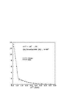
Figure 5: Cross sections for SM (left panels) and for $h^{0}$ in S1 MSSM (right panels). BSM and MSSM parameters as in previous figures.

In the left panels of Fig.5 we give the unpolarized differential cross sections for $H_{SM}$ in SM. Correspondingly in the right panels of Fig.5 we present the $h^{0}$ production in S1 MSSM [24]. In the various panels we show the energy and angular dependencies, as in Figs.1-4.

Note that the angular peaks in the forward and backward directions (coming from $t,u$ channel triangles and boxes) and the CP invariance of the one loop contributions lead to forward-backward symmetries, possibly violated by anomalous couplings.

6.3 $A_{LR}$ Asymmetries

We first discuss $A_{LR}$ defined in (21) for the case where the polarization of the final photon is not measured. In Fig.6 we give $A_{LR}$ for $H_{SM}$ (left panels) and the MSSM $h^{0}$ results (right panels). The one loop contributions $A_{LR}$ get large values. The weak energy and angle dependencies come from the dominance of the L amplitudes as seen above. The $H_{SM}$ and $h^{0}$ cases are rather similar.

The BSM contributions from W eff and B eff (17, 18), are also large and rather flat.

We next turn $A_{LR}(\tau)$ defined in (22) for the cases the polarization of the final photon is chosen to have specific values $\tau=\pm 1$. Fig.7 show $A_{LR}$ for $\tau=+1$, and Fig.8 for $\tau=-1$.

The angular dependencies are particularly interesting. For the one loop amplitudes which respect CP-invariance, they reflect the helicity properties of (30). Consequently, the two $\tau$-helicity one-loop $A_{LR}(\tau)$ satisfy an F/B interchange rule. But this is strongly violated by the chosen BSM anomalous couplings, which do not respect CP invariance.

6.4 $A^{{\rm pol}~{}\gamma}$ Asymmetries

For unpolarized $e^{\pm}$ beams, these are defined in (23) and shown in Figs.9 for $H_{SM}$ (left panels) and $h^{0}$ (right panels).

As seen there, the energy dependence is not negligible and the angular dependencies reflect also the photon helicity properties of the one loop terms. CP invariance imposes the F/B antisymmetry, again possibly perturbed by anomalous coupling contributions.

The corresponding results for $e^{-}_{L}$ and $e^{-}_{R}$-beams, defined in (24), are shown in Fig.10 for $H_{SM}$ (left panels) and $h^{0}$ (right panels).

These 2 cases of electron polarization lead to very different results; they can even differ by a sign. As the L amplitudes are larger than the R ones, this explains why this case leads to results closer to the unpolarized ones.

The CP forward-backward symmetry relations of (31) are well illustrated and again easily violated by anomalous couplings.

6.5 Azimuthal dependence

As described in Sect.5, when transversely polarized beams are available, the azimuthal dependence of the differential cross section is controlled by the coefficients $T_{\cos 2\phi}$, $T_{\sin 2\phi}$ in (37), of the $\cos 2\phi$, $\sin 2\phi$ terms in (32). Fig.11 then shows the energy and angular dependencies for $H_{SM}$ (left panels) and $h^{0}$ (right panels).

These coefficients get non negligible values which means that there is a significant azimuthal dependence. As already mentioned $T_{\sin 2\phi}$ is particularly interesting because it is governed by the imaginary parts of the amplitudes which are important in the process under consideration. This should constitute an additional source of tests of the underlying dynamics and of the Higgs couplings. With CP invariance the angular dependence of these coefficients is forward-backward symmetric.

In the left panels of Fig.11, we also show the contributions of the anomalous couplings of W and B types (17, 18).

7 Conclusions

We have analyzed the specificity of the process $e^{-}e^{+}\to\gamma H$ as compared to $e^{-}e^{+}\to ZH$. The new feature is that this process has no Born term and is therefore immediately sensitive to one loop effects and the underlying Higgs dynamics. This arises in particular through the contributions of the imaginary parts of the amplitudes.

Our aim in doing this, is to see the differences between SM, MSSM and another (possibly CP violating) BSM, and to check especially whether this is observable when using the supersimple approximation.

We have insisted on two important aspects of the supersimple description. Its ability to allow the immediate reading of the dynamical contents of the various standard and non standard contributions. And in addition, the fact that these supersimple expressions quite accurately reproduce the exact one loop effects at high energies.

For achieving this, we have computed the exact one loop amplitudes and cross sections, as well as their sim approximations, and compared them numerically. The sim and exact one loop amplitudes agree at high energy, but differ at low energies due to neglected terms behaving like $m^{2}/s$, possibly modified by logarithmic corrections, and also due to threshold effects caused by virtual contributions particularly visible in the SUSY cases.

At 1 TeV, the agreement between sim and the exact one loop results, is already good in the $H_{SM}$ case, but there are still some non negligible differences in the $h^{0}$ case, which disappear at higher energies. The $H^{0}$ case would need even higher energies for achieving such an accuracy; but $H^{0}$ production is probably unobservable with the considered benchmark parameters [24].

In addition to the unpolarized differential cross section (angular distribution and forward-backward asymmetry) we have also considered several other observables with initial and final polarization asymmetries: $A_{LR}$, $A_{LR}(\tau=\mp 1)$, $A^{{\rm pol}~{}\gamma}$, $A^{{\rm pol}~{}\gamma}_{L}$ , $A^{{\rm pol}~{}\gamma}_{R}$; as well as the coefficients of the $\cos 2\phi$ and $\sin 2\phi$ azimuthal dependencies (37), when the $e^{\pm}$ beams are transversally polarized.

We have illustrated how sensitive all these observables are to the underlying dynamics by comparing the SM predictions to the MSSM ones, and a simple type of BSM physics involving anomalous Higgs couplings to gauge bosons, possibly containing also CP violation.

We hope that this work will motivate further studies studies of the $e^{-}e^{+}\to\gamma H$ process, using in particular polarized beams and containing also measurements of the final $\gamma$ polarization.

Appendix: Sim expressions for the $e^{-}e^{+}\to\gamma H$ amplitudes in SM and MSSM

From the decomposition of the invariant amplitude over the CP-conserving invariant forms defined in (4) and leading to (9), we write the four HV amplitudes in the form

$$F_{--} = {\alpha^{2}m_{W}\over\beta_{\gamma}}\left[{u\sqrt{2}\over\sqrt{s}}N^{L}_{1}+{ut\over\sqrt{2s}}(N^{L}_{3}-N^{L}_{4})\right]~{}~{},$$

$$F_{+-} = {\alpha^{2}m_{W}\over\beta_{\gamma}}\left[{t\sqrt{2}\over\sqrt{s}}N^{R}_{1}-{ut\over\sqrt{2s}}(N^{R}_{3}-N^{R}_{4})\right]~{}~{},$$

$$F_{-+} = {\alpha^{2}m_{W}\over\beta_{\gamma}}\left[{t\sqrt{2}\over\sqrt{s}}N^{L}_{1}-{ut\over\sqrt{2s}}(N^{L}_{3}-N^{L}_{4})\right]~{}~{},$$

$$F_{++} = {\alpha^{2}m_{W}\over\beta_{\gamma}}\left[{u\sqrt{2}\over\sqrt{s}}N^{R}_{1}+{ut\over\sqrt{2s}}(N^{R}_{3}-N^{R}_{4})\right]~{}~{},$$ (A.1)

where $H=H_{SM},h^{0},H^{0}$ and the kinematics are defined in (2).

The $N^{L,R}_{i}$ contributions in (A.1) are obtained from the exact 1 loop computation in terms of PV functions [11]. These are then expanded using the high energy forms given in [12]. We thus obtain the so called supersimple (sim) results written below in SM and MSSM.

We next turn to the forms entering the sim expressions. These consist of the linear log augmented Sudakov form and the forms involving ratios of Mandelstam variables, as in [5, 13, 15]. These are

$$\overline{\ln s_{ij}(a)}\equiv\ln{-s-i\epsilon\over m_{i}m_{j}}+b_{0}^{ij}(m^{2}_{a})-2~{}~{},$$ (A.2)

where $b_{0}^{ij}(m^{2}_{a})$ is given in e.g. Eqs.(A.6) of [15], with (i,j) denoting internal exchanges and $a$ an on-shell particle, such that the $aij$ tree level coupling is non vanishing. And the forms

$$\overline{\ln^{2}r_{xy}}=\ln^{2}r_{xy}+\pi^{2}~{}~{}~{},~{}~{}~{}\ln r_{xy}~{}~{}~{}.~{}~{}$$ (A.3)

where

$$r_{xy}\equiv\frac{-x-i\epsilon}{-y-i\epsilon}~{}~{},$$ (A.4)

with $x,y$ standing for the Mandelstam-variables $s,t,u$.

For $e^{-}e^{+}\to\gamma H$ though, the additional augmented quadratic Sudakov logarithms though, are different from those in [5, 13, 15]. The forms we meet here are

$$\overline{\ln^{2}x_{WW}}=\ln^{2}{-x-i\epsilon\over m^{2}_{W}}+2L_{\gamma WW}+2L_{HWW}~{}~{},$$

$$\overline{\ln^{2}x_{W}}=\ln^{2}{-x-i\epsilon\over m^{2}_{W}}+2L_{eW\nu}+L_{\gamma WW}+L_{HWW}~{}~{},$$

$$\overline{\ln^{2}x_{Z}}=\ln^{2}{-x-i\epsilon\over m^{2}_{Z}}+2L_{eZe}+L_{HZZ}~{}~{},$$

$$\overline{\ln^{2}x_{t}}=\ln^{2}{-x-i\epsilon\over m^{2}_{t}}+2L_{\gamma tt}+2L_{Htt}~{}~{},$$

$$\overline{\ln^{2}x_{b}}=\ln^{2}{-x-i\epsilon\over m^{2}_{b}}+2L_{\gamma tt}+2L_{Hbb}~{}~{},$$ (A.5)

and the forms involving charginos or neutralinos described by the indices $(i,j,k)$ and given by

$$\overline{\ln^{2}x_{j}}=\ln^{2}{-x-i\epsilon\over M^{2}_{j}}+2L_{Hji}+2L_{ej\tilde{l}_{L}}~{}~{}{\rm~{}with}~{}~{}~{}\tilde{l}_{L}=\tilde{\nu}_{L}~{},~{}\tilde{e}_{L}~{},$$

$$\overline{\ln^{2}s_{ii}}=\ln^{2}{s\over M^{2}_{i}}+2L_{\gamma ii}+2L_{Hii}~{}~{},~{}~{}\overline{\ln^{2}s_{ji}}=\ln^{2}{s\over M^{2}_{j}}+2L_{\gamma jj}+2L_{Hji}~{},$$ (A.6)

where $L_{aij}$ in (A.5, A.6) are given in Eqs.(22) of [12]. Again (i,j) denote internal exchanges and $a$ an on-shell external particle, such that the $aij$ tree level coupling is non vanishing.

To describe the sim expressions, we also need the constants of Table A.1, the $(t,b)$ and sfermion couplings respectively given by

$$C^{L}_{t}={-3-2s^{2}_{W}\over 3s^{2}_{W}c^{2}_{W}}~{},~{}C^{L}_{b}={-3+2s^{2}_{W}\over 6s^{2}_{W}c^{2}_{W}}~{},~{}C^{R}_{t}={-10\over 3c^{2}_{W}}~{},~{}C^{R}_{b}={-1\over 3c^{2}_{W}}~{}~{},$$ (A.7)

$$f_{Z\tilde{f}}=-{(I^{3}_{\tilde{f}}-s^{2}_{W}Q_{\tilde{f}})\over s_{W}c_{W}}~{},~{}f_{H\tilde{f}}={m_{W}(I^{3}_{\tilde{f}}-s^{2}_{W}Q_{\tilde{f}})\over s_{W}c^{2}_{W}}C^{+}_{H}-{m^{2}_{f}\over s_{W}m_{W}}f_{fH}~{},$$ (A.8)

as well as the chargino and neutralino couplings

$$A^{L}_{i}(\tilde{e}_{L})=-~{}{e\over s_{W}}Z^{-}_{1i}~{}~{},~{}~{}A^{L}_{i}(\tilde{\nu}_{L})=-~{}{e\over s_{W}}Z^{+}_{1i}$$

$$A^{0L}_{i}(\tilde{e}_{L})={e\over\sqrt{2}s_{W}c_{W}}(Z^{N}_{1i}s_{W}+Z^{N}_{2i}c_{W})~{}~{},~{}~{}A^{0R}_{i}(\tilde{e}_{R})=-{e\sqrt{2}\over c_{W}}Z^{N*}_{1i}$$

$$O^{L}_{Zij}=-{1\over 2s_{W}c_{W}}(Z^{+*}_{1i}Z^{+}_{1j}+\delta_{ij}(c^{2}_{W}-s^{2}_{W}))~{},$$

$$O^{R}_{Zij}=-{1\over 2s_{W}c_{W}}(Z^{-}_{1i}Z^{-*}_{1j}+\delta_{ij}(c^{2}_{W}-s^{2}_{W}))~{},$$

$$c^{L}_{h^{0}ij}=-{1\over\sqrt{2}s_{W}}(-\sin\alpha Z^{-}_{2i}Z^{+}_{1j}+\cos\alpha Z^{-}_{1i}Z^{+}_{2j})~{}~{},~{}~{}c^{R}_{h^{0}ij}=c^{L*}_{h^{0}ji}~{},$$

$$O^{0L}_{Zij}={1\over 2s_{W}c_{W}}(Z^{N*}_{4i}Z^{N}_{4j}-Z^{N*}_{3i}Z^{N}_{3j})~{}~{},~{}~{}O^{R}_{Zij}={1\over 2s_{W}c_{W}}(Z^{N}_{3i}Z^{N*}_{3j}-Z^{N}_{4i}Z^{N*}_{4j})~{},$$

$$c^{0L}_{h^{0}ij}={1\over 2s_{W}c_{W}}[(-\sin\alpha Z^{N}_{3i}-\cos\alpha Z^{N}_{4j})(Z^{N}_{1i}s_{W}-Z^{N}_{2i}c_{W}))+(i\to j)]~{},~{}$$

$$c^{0R}_{h^{0}ij}=c^{0L*}_{h^{0}ji},$$ (A.9)

given in terms of the usual mixing matrices [25].

Table A.1: Parameters for the HV amplitudes in SM and MSSM

	$H_{SM}$	$h^{0}$	$H^{0}$
$C^{-}_{H}$	1	$\sin(\beta-\alpha)$	$\cos(\beta-\alpha)$
$C^{+}_{H}$	0	$\sin(\beta+\alpha)$	$-\cos(\beta+\alpha)$
$f_{GGH}$	$-{m^{2}_{H}\over 2s_{W}m_{W}}$	${m_{W}\over 2s_{W}c^{2}_{W}}\cos(2\beta)\sin(\beta+\alpha)$	- ${m_{W}\over 2s_{W}c^{2}_{W}}\cos(2\beta)\cos(\beta+\alpha)]$
$f_{HHH}$	0	$-{m_{W}\over s_{W}}\left[{\cos(2\beta)\sin(\beta+\alpha)\over 2c^{2}_{W}}+\sin(\beta-\alpha)\right]$	${m_{W}\over s_{W}}\left[{\cos(2\beta)\cos(\beta+\alpha)\over 2c^{2}_{W}}-\cos(\beta-\alpha)\right]$
$f_{tH}$	1	${\cos\alpha\over\sin\beta}$	${\sin\alpha\over\sin\beta}$
$f_{bH}$	1	$-{\sin\alpha\over\cos\beta}$	${\cos\alpha\over\cos\beta}$

The $H^{0}$-case is subsequently obtained from the above $h^{0}$-one through the replacement

$$(~{}h^{0}\Rightarrow H^{0}~{})\mapsto(\sin\alpha\Rightarrow-\cos\alpha~{}~{}~{},~{}~{}~{}\cos\alpha\Rightarrow\sin\alpha)~{}~{}.$$ (A.10)

Using the above forms and couplings, we give below the sim results for the $N^{L,R}_{i}$ contributions to the HV amplitudes in (A.1). These include an SM part which is easily identified, and the MSSM SUSY contributions to the $h^{0}$ case, arising from sfermion and chargino-neutralino exchanges.

In the expressions below, the SM and sfermion contributions are always included explicitly in the $N^{L,R}_{i}$-forms, while the chargino-neutralino contributions are collected in $T$ and $B$ forms entering them. We thus have

$$sN^{L}_{1}=C^{-}_{H}\left\{{\overline{\ln^{2}s_{WW}}\over 2c^{2}_{W}s^{3}_{W}}-{1+4c^{2}_{W}\over 4s^{3}_{W}c^{2}_{W}}[\overline{\ln s_{WW}(H)}+\overline{\ln s_{WW}(\gamma)}]+{1\over 2s^{3}_{W}c^{2}_{W}}\right\}$$

$$-{(f_{GGH}+f_{HHH})\over 2c^{2}_{W}s^{2}_{W}m_{W}}\Big{[}1-{1\over 2}[\overline{\ln s_{WW}(H)}+\overline{\ln s_{WW}(\gamma)}]\Big{]}$$

$$+{m^{2}_{t}\over s_{W}m^{2}_{W}}C^{L}_{t}f_{tH}\left[{\overline{\ln^{2}s_{t}}\over 4}-{1\over 2}\Big{(}\overline{\ln s_{tt}(H)}+\overline{\ln s_{tt}(\gamma)}\Big{)}+1\right]$$

$$+{m^{2}_{b}\over s_{W}m^{2}_{W}}C^{L}_{b}f_{bH}\left[{\overline{\ln^{2}s_{b}}\over 4}-{1\over 2}\Big{(}\overline{\ln s_{bb}(H)}+\overline{\ln s_{bb}(\gamma)}\Big{)}+1\right]$$

$$-\frac{sC^{-}_{H}}{s^{3}_{W}}\left\{{\overline{\ln t_{WW}(H)}\over t}+{\overline{\ln u_{WW}(H)}\over u}+{(2s^{2}_{W}-1)^{2}\over 2c^{3}_{W}}\left[{\overline{\ln t_{ZZ}(H)}\over t}+{\overline{\ln u_{ZZ}(H)}\over u}\right]\right\}$$

$$-{2\over m_{W}}\Sigma_{\tilde{f}}Q_{\tilde{f}}f_{H\tilde{f}}\left[Q_{\tilde{f}}+{(2s^{2}_{W}-1)\over 2s_{W}c_{W}}f_{Z\tilde{f}}\right]\left[1-{1\over 2}\left(\overline{\ln s_{\tilde{f}\tilde{f}}}(H)+\overline{\ln s_{\tilde{f}\tilde{f}}}(\gamma)\right)\right]$$

$$+{sC^{+}_{H}\over 2c^{2}_{W}s_{W}^{3}}\left\{{\overline{\ln t_{\tilde{\nu}\tilde{\nu}}}(H)\over t}+{\overline{\ln u_{\tilde{\nu}\tilde{\nu}}}(H)\over u}+{(2s^{2}_{W}-1)\over 2c^{2}_{W}}\left[{\overline{\ln t_{\tilde{e_{L}}\tilde{e_{L}}}}(H)\over t}+{\overline{\ln u_{\tilde{e_{L}}\tilde{e_{L}}}}(H)\over u}\right]\right\}$$

$$+\frac{C^{-}_{H}}{2s^{3}_{W}}\Bigg{\{}{s\over t}(\overline{\ln^{2}t_{W}}-\overline{\ln^{2}r_{us}})+{s\over u}(\overline{\ln^{2}u_{W}}-\overline{\ln^{2}r_{ts}})$$

$$+{(1-2s^{2}_{W})^{2}\over 2c^{4}_{W}}\Big{[}{s\over u}\overline{\ln^{2}u_{Z}}+{s\over t}\overline{\ln^{2}t_{Z}}+2\overline{\ln^{2}r_{tu}}\Big{]}\Bigg{\}}$$

$$-{(1-2s^{2}_{W})C^{+}_{H}\over 8s^{3}_{W}c^{4}_{W}}\left[{s\over u}\overline{\ln^{2}r_{ts}}+{s\over t}\overline{\ln^{2}r_{us}}\right]+T^{L1}_{\chi\chi}+T^{L1}_{\chi\chi\chi}+B^{L1}_{\chi\chi}+B^{L1}_{\chi\chi\chi}~{},$$ (A.11)

with the chargino-neutralino contributions being

$$T^{L1}_{\chi\chi}=\sum_{\chi^{+}_{i}\chi^{+}_{j}}A^{L*}_{j}(\tilde{\nu}_{L})A^{L}_{i}(\tilde{\nu}_{L})\Big{[}{M_{j}\over m_{W}}c^{R}_{Hji}{s\over 2t}(\overline{\ln^{2}t_{j}}-2\overline{\ln t_{ji}(H)})-{M_{i}\over m_{W}}c^{L}_{Hji}{s\over t}(\overline{\ln t_{ji}(H)})$$

$$+{M_{j}\over m_{W}}c^{L}_{Hij}{s\over 2u}(\overline{\ln^{2}u_{j}}-2\overline{\ln u_{ji}(H)})-{M_{i}\over m_{W}}c^{R}_{Hij}{s\over u}(\overline{\ln u_{ji}(H)})\Big{]}$$

$$+\sum_{\chi^{0}_{i}\chi^{0}_{j}}A^{0L*}_{j}(\tilde{e}_{L})A^{0L}_{i}(\tilde{e}_{L})\Big{[}{M_{j}\over m_{W}}c^{0R}_{Hji}{s\over 2t}(\overline{\ln^{2}t_{j}}-2\overline{\ln t_{ji}(H)})-{M_{i}\over m_{W}}c^{0L}_{Hji}{s\over t}(\overline{\ln t_{ji}(H)})$$

$$+{M_{j}\over m_{W}}c^{0L}_{Hij}{s\over 2u}(\overline{\ln^{2}u_{j}}-2\overline{\ln u_{ij}(H)})-{M_{i}\over m_{W}}c^{0R}_{Hij}{s\over u}(\overline{\ln u_{ij}(H)})\Big{]}~{},$$

$$T^{L1}_{\chi\chi\chi}=-\sum_{\chi^{+}_{i}\chi^{+}_{j}}{4\over m_{W}}\Bigg{\{}2Q_{e}c^{L}_{Hii}M_{i}\left[{1\over 4}\overline{\ln^{2}s_{ii}}-\overline{\ln s_{ii}(H)}+1\right]$$

$$+g^{L}_{Ze}(O^{R}_{Zij}+O^{L}_{Zij})c^{L}_{Hji}M_{i}\left[{1\over 4}\overline{\ln^{2}s_{ji}}-\overline{\ln s_{ij}(H)}+1\right]\Bigg{\}}~{},$$

$$B^{L1}_{\chi\chi}=\sum_{\chi^{0}_{i}\chi^{0}_{j}}A^{L0*}_{j}(\tilde{e}_{L})A^{L0}_{i}(\tilde{e}_{L})\left[{M_{i}\over 2m_{W}}c^{0L}_{Hji}+{M_{j}\over 2m_{W}}c^{0R}_{Hji}\right]\overline{\ln^{2}r_{tu}}~{},$$

$$B^{L1}_{\chi\chi\chi}=\sum_{\chi^{+}_{i}\chi^{+}_{k}}{M_{k}\over m_{W}}c^{R}_{Hki}A^{L*}_{k}(\tilde{\nu}_{L})A^{L}_{i}(\tilde{\nu}_{L})\left[\overline{\ln^{2}s_{ki}}+{s\over u}\overline{\ln^{2}r_{ts}}+{s\over t}\overline{\ln^{2}r_{us}}\right]~{},$$ (A.12)

and

$$N^{L}_{3}-N^{L}_{4}=-C^{-}_{H}\Bigg{\{}{2\over s^{3}_{W}}\Big{[}{(t-u)\over 2tu}\overline{\ln^{2}s_{WW}}+{\overline{\ln^{2}t_{W}}\over 4t}-{\overline{\ln^{2}u_{W}}\over 4u}$$

$$+{s\overline{\ln r_{tu}}\over ut}+{(2u^{2}-2t^{2}+ut)\over 4tu^{2}}\overline{\ln^{2}r_{ts}}+{(2u^{2}-2t^{2}-ut)\over 4ut^{2}}\overline{\ln^{2}r_{us}}\Big{]}$$

$$+{1\over 2s^{3}_{W}}\Big{[}{\overline{\ln^{2}u_{W}}\over u}-{\overline{\ln^{2}t_{W}}\over t}+{\overline{\ln^{2}r_{us}}\over t}-{\overline{\ln^{2}r_{ts}}\over u}\Big{]}$$

$$+{(2s_{W}^{2}-1)^{2}\over 2c^{4}_{W}s^{3}_{W}}\Big{[}{s\over ut}(\overline{\ln^{2}t_{Z}}-\overline{\ln^{2}u_{Z}})+{2s\over ut}(\overline{\ln u_{ZZ}(H)}-\overline{\ln t_{ZZ}(H)})$$

$$+{\overline{\ln^{2}r_{tu}}\over u}-{\overline{\ln^{2}r_{tu}}\over t}\Big{]}\Bigg{\}}+{{(2s^{2}_{W}-1)\over 4s^{3}_{W}c^{4}_{W}}}C^{+}_{H}\Big{[}{s\overline{\ln^{2}r_{ts}}\over u^{2}}-{s\overline{\ln^{2}r_{us}}\over t^{2}}+2s{\overline{\ln r_{ts}}-\overline{\ln r_{us}}\over ut}\Big{]}$$

$$+{1\over s^{3}_{W}c^{2}_{W}}C^{+}_{H}{s\overline{\ln r_{tu}}\over tu}+B^{L34}_{\chi\chi}+B^{L34}_{\chi\chi\chi}~{}~{},$$ (A.13)

with

$$B^{L34}_{\chi\chi}=\sum_{\chi^{0}_{i}\chi^{0}_{j}}A^{L0*}_{j}(\tilde{e}_{L})A^{L0}_{i}(\tilde{e}_{L})\Bigg{\{}{M_{i}\over m_{W}}c^{0L}_{Hji}\Big{[}-{s\overline{\ln^{2}u_{i}}\over ut}-2s{\overline{\ln r_{tu}}\over ut}-{\overline{\ln^{2}r_{tu}}\over t}\Big{]}$$

$$+{M_{j}\over m_{W}}c^{0R}_{Hji}\Big{[}{s\overline{\ln^{2}t_{j}}\over ut}-2s{\overline{\ln r_{tu}}\over ut}+{\overline{\ln^{2}r_{tu}}\over u}\Big{]}\Bigg{\}}~{},$$

$$B^{L34}_{\chi\chi\chi}=\sum_{\chi^{+}_{i}\chi^{+}_{k}}{M_{k}\over m_{W}}c^{R}_{Hki}A^{L*}_{k}(\tilde{\nu}_{L})A^{L}_{i}(\tilde{\nu}_{L})\Bigg{[}{\overline{\ln^{2}s_{ik}}\over t}-{\overline{\ln^{2}s_{ki}}\over u}+{4s\overline{\ln r_{ut}}\over ut}$$

$$+{(2t^{2}-u^{2}+tu)\over tu^{2}}\overline{\ln^{2}r_{ts}}-~{}{(2u^{2}-t^{2}+tu)\over ut^{2}}\overline{\ln^{2}r_{us}}\Bigg{]}~{},$$ (A.14)

and

$$sN^{R}_{1}=C^{-}_{H}\Big{[}{\overline{\ln^{2}s_{WW}}+1-{1\over 2}(\overline{\ln s_{WW}(H)}+\overline{\ln s_{WW}(\gamma)})\over s_{W}c^{2}_{W}}\Big{]}$$

$$-{(f_{GGH}+f_{HHH})\over c^{2}_{W}m_{W}}\Big{[}1-{1\over 2}(\overline{\ln s_{WW}(H)}+\overline{\ln s_{WW}(\gamma)})\Big{]}$$

$$+{m^{2}_{t}\over s_{W}m^{2}_{W}}C^{R}_{t}f_{tH}\Big{[}{\overline{\ln^{2}s_{t}}\over 4}-{1\over 2}(\overline{\ln s_{tt}(H)}+\overline{\ln s_{tt}(\gamma)})+1\Big{]}$$

$$+{m^{2}_{b}\over s_{W}m^{2}_{W}}C^{R}_{b}f_{bH}\Big{[}{\overline{\ln^{2}s_{b}}\over 4}-{1\over 2}(\overline{\ln s_{bb}(H)}+\overline{\ln s_{bb}(\gamma)})+1\Big{]}$$

$$+C^{-}_{H}\Big{\{}{-2s_{W}\over c^{4}_{W}}\Big{[}{s\overline{\ln t_{ZZ}(H)}\over t}+{s\overline{\ln u_{ZZ}(H)}\over u}\Big{]}+{s_{W}\over c^{4}_{W}}\Big{[}{s\overline{\ln^{2}t_{W}}\over t}+{s\overline{\ln^{2}u_{W}}\over u}+2\overline{\ln^{2}r_{tu}}\Big{]}\Big{\}}$$

$$-{2s_{W}\over c^{4}_{W}}C^{+}_{H}\Big{[}{s\overline{\ln t_{\tilde{e_{R}}\tilde{e_{R}}}}(H)\over t}+{s\overline{\ln u_{\tilde{e_{R}}\tilde{e_{R}}}}(H)\over u}\Big{]}$$

$$-{2\over m_{W}}\Sigma_{\tilde{f}}Q_{\tilde{f}}f_{H\tilde{f}}\Big{[}Q_{\tilde{f}}+{s_{W}\over c_{W}}f_{Z\tilde{f}}\Big{]}\Big{[}1-{1\over 2}(\overline{\ln s_{\tilde{f}\tilde{f}}}(H)+\overline{\ln s_{\tilde{f}\tilde{f}}}(\gamma))\Big{]}$$

$$-{s_{W}\over c^{4}_{W}}C^{+}_{H}\Big{[}{s\over u}\overline{\ln^{2}r_{ts}}+{s\over t}\overline{\ln^{2}r_{us}}\Big{]}+T^{R1}_{\chi\chi}+T^{R1}_{\chi\chi\chi}+B^{R1}_{\chi\chi}~{}~{},$$ (A.15)

with

$$T^{R1}_{\chi\chi}=\sum_{\chi^{0}_{i}\chi^{0}_{j}}A^{0R*}_{j}(\tilde{e}_{R})A^{0R}_{i}(\tilde{e}_{R})\Bigg{[}{M_{j}\over m_{W}}c^{0L}_{Hji}{s\over 2t}(\overline{\ln^{2}t_{j}}-2\overline{lnt_{ji}(H)})-{M_{i}\over m_{W}}c^{0R}_{Hji}{s\over t}(\overline{\ln t_{ji}(H)})$$

$$+{M_{j}\over m_{W}}c^{0R}_{Hij}{s\over 2u}(\overline{\ln^{2}u_{j}}-2\overline{\ln u_{ij}(H)})-{M_{i}\over m_{W}}g^{L}_{Hij}{s\over u}(\overline{\ln u_{ij}(H)})\Bigg{]}~{},$$

$$T^{R1}_{\chi\chi\chi}=-\sum_{\chi^{+}_{i}\chi^{+}_{j}}{4\over m_{W}}\Bigg{\{}2Q_{e}c^{L}_{Hii}M_{i}\Big{[}{1\over 4}\overline{\ln^{2}s_{ii}}-\overline{\ln s_{ii}(H)}+1\Big{]}$$

$$+g^{R}_{Ze}(O^{R}_{Zij}+O^{L}_{Zij})c^{L}_{Hji}M_{i}\Big{[}{1\over 4}\overline{\ln^{2}s_{ji}}-\overline{\ln s_{ij}(H)}+1\Big{]}\Bigg{\}}~{},$$

$$B^{R1}_{\chi\chi}=\sum_{\chi^{0}_{i}\chi^{0}_{j}}A^{0R*}_{j}(\tilde{e}_{R})A^{0R}_{i}(\tilde{e}_{R})\Big{[}{M_{i}\over 2m_{W}}c^{0R}_{Hji}+{M_{j}\over 2m_{W}}c^{0L}_{Hji}\Big{]}\overline{\ln^{2}r_{tu}}~{},$$ (A.16)

and

$$N^{R}_{3}-N^{R}_{4}={2s_{W}\over c^{4}_{W}}C^{-}_{H}\Bigg{[}{s(\overline{\ln^{2}t_{Z}}-\overline{\ln^{2}u_{Z}})\over ut}+2s\Big{[}{\overline{\ln u_{ZZ}(H)}-\overline{\ln t_{ZZ}(H)}\over ut}\Big{]}$$

$$+{\overline{\ln^{2}r_{tu}}\over u}-{\overline{\ln^{2}r_{tu}}\over t}\Bigg{]}-{2s_{W}\over c^{4}_{W}}C^{+}_{H}\Big{[}{s\overline{\ln^{2}r_{ts}}\over u^{2}}-{s\overline{\ln^{2}r_{us}}\over t^{2}}+2s{\overline{\ln r_{ts}}-\overline{\ln r_{us}}\over ut}\Big{]}$$

$$+B^{R34}_{\chi\chi}~{}~{},$$ (A.17)

with

$$B^{R34}_{\chi\chi}=\sum_{\chi^{0}_{i}\chi^{0}_{j}}A^{0R*}_{j}(\tilde{e}_{R})A^{0R}_{i}(\tilde{e}_{R})\Bigg{\{}{M_{i}\over m_{W}}c^{0R}_{Hji}\Big{[}-{s\overline{\ln^{2}u_{i}}\over ut}-2s{\overline{\ln r_{tu}}\over ut}-{\overline{\ln^{2}r_{tu}}\over t}]$$

$$+{M_{j}\over m_{W}}c^{0L}_{Hji}[{s\overline{\ln^{2}t_{j}}\over ut}-2s{\overline{\ln r_{tu}}\over ut}+{\overline{\ln^{2}r_{tu}}\over u}\Big{]}\Bigg{\}}~{}~{}.$$ (A.18)

A rough approximation for the chargino and neutralino contributions in (A.12, A.14, A.16, A.18) is respectively given by neglecting the various mass differences in the summations over virtual states, using common ”average” masses. From the unitarity of the mixing matrices one then obtains the results

$$T^{L1}_{\chi\chi} \simeq \Big{\{}-{<M^{+}_{12}>\sin\alpha\over\sqrt{2}s^{3}_{W}m_{W}}+{(1-2s^{2}_{W})\over 4s^{3}_{W}c^{3}_{W}}{<M^{0}_{L+}>\over m_{W}}\Big{\}}\Big{[}{s\overline{\ln^{2}t}\over 2t}$$

$$-2{s\overline{\ln t}\over t}+{s\overline{\ln^{2}u}\over 2u}-2{s\overline{\ln u}\over u}\Big{]}~{},$$

$$T^{L1}_{\chi\chi\chi} \simeq -{4\over m_{W}}\Big{[}{1\over 4}\overline{\ln^{2}s}-\overline{\ln s}+1\Big{]}\Big{\{}{\sqrt{2}\over s_{W}}+{(2s^{2}_{W}-1)(1-4c^{2}_{W})\over 4\sqrt{2}s^{3}_{W}c^{2}_{W}}\Big{\}}$$

$$\cdot\Big{(}<M^{+}_{21}>\cos\alpha-<M^{+}_{12}>\sin\alpha\Big{)}~{},$$

$$B^{L1}_{\chi\chi} \simeq {(1-2s^{2}_{W})\over 4s^{3}_{W}c^{3}_{W}}{<M^{0}_{L+}>\over m_{W}}\overline{\ln^{2}r_{tu}}~{},$$

$$B^{L1}_{\chi\chi\chi} \simeq {<M^{+}_{12}>\sin\alpha\over\sqrt{2}s^{3}_{W}m_{W}}\left[\overline{\ln^{2}s}+{s\over u}\overline{\ln^{2}r_{ts}}+{s\over t}\overline{\ln^{2}r_{us}}\right]~{}~{},$$

$$B^{L34}_{\chi\chi} \simeq {(1-2s^{2}_{W})\over 4s^{3}_{W}c^{3}_{W}}{<M^{0}_{L+}>\over m_{W}}\left[{s\overline{\ln^{2}t}\over ut}-{s\overline{\ln^{2}u}\over ut}-4s{\overline{\ln r_{tu}}\over ut}+{\overline{\ln^{2}r_{tu}}\over u}-{\overline{\ln^{2}r_{tu}}\over t}\right]~{},$$

$$B^{L34}_{\chi\chi\chi} \simeq -{<M^{+}_{12}>\sin\alpha\over\sqrt{2}s^{3}_{W}m_{W}}\Big{[}{\overline{\ln^{2}s}\over t}-{\overline{\ln^{2}s}\over u}+{4s\overline{\ln r_{ut}}\over ut}+{2t^{2}-u^{2}+tu\over tu^{2}}\overline{\ln^{2}r_{ts}}$$

$$-~{}{2u^{2}-t^{2}+tu\over ut^{2}}\overline{\ln^{2}r_{us}}\Big{]}~{},$$

$$T^{R1}_{\chi\chi} \simeq -~{}{1\over c^{3}_{W}}{<M^{0}_{R-}>\over m_{W}}\Big{[}{s\overline{\ln^{2}t}\over 2t}-2{s\overline{\ln t}\over t}+{s\overline{\ln^{2}u}\over 2u}-2{s\overline{\ln u}\over u}\Big{]}~{},$$

$$T^{R1}_{\chi\chi\chi} \simeq -{4\over m_{W}}\Big{\{}{\sqrt{2}\over s_{W}}+{1-4c^{2}_{W}\over 2\sqrt{2}s_{W}c^{2}_{W}}\Big{\}}\Big{[}{1\over 4}\overline{\ln^{2}s}-\overline{\ln s}+1\Big{]}(<M^{+}_{21}>\cos\alpha$$

$$-<M^{+}_{12}>\sin\alpha)~{},$$

$$B^{R1}_{\chi\chi} \simeq -~{}{<M^{0}_{R+}>\over c^{3}_{W}m_{W}}\overline{\ln^{2}r_{tu}}~{},$$

$$B^{R34}_{\chi\chi} \simeq -{<M^{0}_{R+}>\over c^{3}_{W}m_{W}}\left[{s\overline{\ln^{2}t}\over ut}-{s\overline{\ln^{2}u}\over ut}-4s{\overline{\ln r_{tu}}\over ut}+{\overline{\ln^{2}r_{tu}}\over u}-{\overline{\ln^{2}r_{tu}}\over t}\right]~{}~{}$$ (A.19)

with

$$<M^{+}_{12}>={m_{W}\sqrt{2}\over\sqrt{1+\tan^{2}\beta}}~{}~{},~{}~{}<M^{+}_{21}>={m_{W}\sqrt{2}\tan\beta\over\sqrt{1+\tan^{2}\beta}}~{}~{},$$

$$<M^{0}_{L+}>=\sin\alpha(s_{W}<M^{N}_{13}>+c_{W}<M^{N}_{23}>)+\cos\alpha(s_{W}<M^{N}_{14}>+c_{W}<M^{N}_{24}>)~{}~{},$$

$$<M^{0}_{L-}>=-\sin\alpha(s_{W}<M^{N}_{13}>+c_{W}<M^{N}_{23}>)+\cos\alpha(s_{W}<M^{N}_{14}>+c_{W}<M^{N}_{24}>)~{}~{},$$

$$<M^{0}_{R-}>=\sin\alpha<M^{N}_{13}>-\cos\alpha<M^{N}_{14}>~{}~{},$$

$$<M^{0}_{R+}>=\sin\alpha<M^{N}_{13}>+\cos\alpha<M^{N}_{14}>~{}~{},$$

$$<M^{{}^{\prime}0+}_{L-}>=\sin\alpha(s_{W}<M^{N}_{13}>-c_{W}<M^{N}_{23}>)+\cos\alpha(s_{W}<M^{N}_{14}>-c_{W}<M^{N}_{24}>)~{}~{},$$

$$<M^{N}_{13}>={-m_{W}s_{W}\over c_{W}\sqrt{1+\tan^{2}\beta}}~{}~{},~{}~{}<M^{N}_{23}>={m_{W}\over\sqrt{1+\tan^{2}\beta}}~{}~{},$$

$$<M^{N}_{14}>={m_{W}s_{W}\tan\beta\over c_{W}\sqrt{1+\tan^{2}\beta}}~{}~{},~{}~{}<M^{N}_{24}>={-m_{W}\tan\beta\over\sqrt{1+\tan^{2}\beta}}~{}~{},$$ (A.20)

where $M^{+\top}$ denotes the $\tilde{\chi}^{+}$ mass matrix, and $M^{N}$ the neutralino one.

The quantities $\overline{\ln^{2}x}$ and $\overline{\ln x}$ in (A.19) are approximated by their pure logarithmic contents $\ln^{2}(x/M^{2})$ and $\ln(x/M^{2})$, where $M$ are adequate average sparticle masses. Correspondingly, the average $<M>$-quantities in (A.20) denote common (chargino or neutralino) mass matrix elements. The values of these average masses could be determined by fitting each B and T contribution in (A.12, A.14, A.16, A.18), to its corresponding (A.19, A.20) simplified expression.

However the numerical results are not very accurate at low energies, because they do not reproduce the various threshold structures. In addition the values of the average masses should be adapted to each specific benchmark choice. In fact the use of the simplified expressions (A.19, A.20) is only to show in a direct way the nature of the $B$ and $T$ contributions. In the numerical calculations it is best to use the expressions in (A.12, A.14, A.16, A.18).

Global approximation for the helicity amplitudes:
Finally we give a global fit of the four helicity amplitudes, which reproduces at intermediate energies (in the domain 0.6-5. TeV), their angular and energy dependencies. The fit is rather accurate, being valid at a few percent level. It consists in fitting the one loop contributions, to the forms

$$F_{--} = {\alpha^{2}m_{W}\over\beta_{g}}\left[{u\sqrt{2}\over s\sqrt{s}}(C^{L}_{1}+C^{\prime L}_{1}\cot^{2}\theta)+{(u-t)\over s\sqrt{2s}}C^{L}_{34}\right]~{}~{}$$

$$F_{+-} = {\alpha^{2}m_{W}\over\beta_{g}}\left[{t\sqrt{2}\over s\sqrt{s}}(C^{R}_{1}+C^{\prime R}_{1}\cot^{2}\theta)-{(u-t)\over s\sqrt{2s}}C^{R}_{34}\right]~{}~{}$$

$$F_{-+} = {\alpha^{2}m_{W}\over\beta_{g}}\left[{t\sqrt{2}\over s\sqrt{s}}(C^{L}_{1}+C^{\prime L}_{1}\cot^{2}\theta)-{(u-t)\over s\sqrt{2s}}C^{L}_{34}\right]~{}~{}$$

$$F_{++} = {\alpha^{2}m_{W}\over\beta_{g}}\left[{u\sqrt{2}\over s\sqrt{s}}(C^{R}_{1}+C^{\prime R}_{1}\cot^{2}\theta)+{(u-t)\over s\sqrt{2s}}C^{R}_{34}\right]~{}~{},$$ (A.21)

with

$$C^{L,R}_{1,34} = a^{L,R}_{1,34}\ln^{2}{s\over m^{2}_{W}}+b^{L,R}_{1,34}\ln{s\over m^{2}_{W}}+c^{L,R}_{1,34}$$

$$C^{\prime L,R}_{1,34} = a^{\prime L,R}_{1,34}\ln^{2}{s\over m^{2}_{W}}+b^{\prime L,R}_{1,34}\ln{s\over m^{2}_{W}}+c^{\prime L,R}_{1,34}~{}~{}.$$ (A.22)

Note the factors $(u-t)$, in front of the $C_{34}$ coefficients in (A.21), which reproduce the fact that these terms, arising only from boxes, vanish at $\theta=\pi/2$, due to crossing relations.

Note also that the terms $C^{\prime L,R}_{1}\cot^{2}\theta$ reproduce the angular dependencies coming from t,u channel triangles and boxes.

The effective constants in (A.21, A.22) are given in Table A.2. Note the similarity of the real parts in the $H_{SM}$ and the $h^{0}$ cases, and the large differences in the imaginary parts, due to the averaging of the threshold effects in the virtual contributions of the spartners.

Table A.2: Constants fitting the amplitudes (A.21, A.22), for SM and S1 MSSM,

in the intermediate anergy domain 0.6-5 TeV [24]

$H_{SM}$
$a^{L}_{1}=-31.4+i5.7$	$b^{L}_{1}=150.3-i21.6$	$c^{L}_{1}=-319.1-i22.4$
$a^{L}_{34}=13.0-i1.8$	$b^{L}_{34}=-54.5-i29.9$	$c^{L}_{34}=47.4+i82.6$
$a^{R}_{1}=-10.9+i3.1$	$b^{R}_{1}=79.6+i3.5$	$c^{R}_{1}=-143.4-i47.4$
$a^{R}_{34}=0.57$	$b^{R}_{34}=-1.26$	$c^{R}_{34}=-0.90$
$a^{\prime L}_{1}=17.7-i1.2$	$b^{\prime L}_{1}=-88.8+i19.2$	$c^{\prime L}_{1}=149.6-i57.9$
$a^{\prime R}_{1}=2.7$	$b^{\prime R}_{1}=-15.3$	$c^{\prime R}_{1}=24.2$
$h^{0}$ S1 MSSM
$a^{L}_{1}=-46.1+i55.2$	$b^{L}_{1}=336.9-i596.4$	$c^{L}_{1}=-832.0+i1482.3$
$a^{L}_{34}=14.2-i1.6$	$b^{L}_{34}=-65.9-i32.2$	$c^{L}_{34}=74.0+i88.4$
$a^{R}_{1}=-12.9+i7.82$	$b^{R}_{1}=114.6-i43.6$	$c^{R}_{1}=-249.2+i61.8$
$a^{R}_{34}=0.40+i0.42$	$b^{R}_{34}=0.42-i3.80$	$c^{R}_{34}=-4.86+i8.52$
$a^{\prime L}_{1}=17.69-i1.60$	$b^{\prime L}_{1}=-88.1+i23.1$	$c^{\prime L}_{1}=146.6-i67.8$
$a^{\prime R}_{1}=2.22+i0.16$	$b^{\prime R}_{1}=-11.2-i1.5$	$c^{\prime R}_{1}=15.3+i3.3$
$H^{0}$ S1 MSSM
$a^{L}_{1}=8.5+i32.2$	$b^{L}_{1}=-61.4-i421.7$	$c^{L}_{1}=102.6+i1176.1$
$a^{L}_{34}=-5.0+i2.7$	$b^{L}_{34}=47.4-i23.0$	$c^{L}_{34}=-109.7+i49.1$
$a^{R}_{1}=-2.1+i1.8$	$b^{R}_{1}=28.9-i27.7$	$c^{R}_{1}=-83.7+i82.0$
$a^{R}_{34}=0.16-i0.043$	$b^{R}_{34}=-1.46+i0.39$	$c^{R}_{34}=3.20-i0.88$
$a^{\prime L}_{1}=0.18+i0.10$	$b^{\prime L}_{1}=-3.36-i2.28$	$c^{\prime L}_{1}=10.7+i7.5$
$a^{\prime R}_{1}=0.24-i0.0064$	$b^{\prime R}_{1}=-2.26+i0.0070$	$c^{\prime R}_{1}=5.13+i0.073$

         

         

         

Figure 1: The $F_{--}$ (left panels) and $F_{++}$ (right panels) amplitudes in SM. Upper row gives the energy dependence at $60^{\circ}$, while the middle (lower) row gives the angular dependence at 1 (5) TeV. The W eff and B eff couplings of the BSM model are defined in (17 , 18).

         

         

         

Figure 2: The $F_{-+}$ (left panels) and $F_{+-}$ (right panels) amplitudes in SM. Panels and BSM couplings as in Fig.1.

         

         

         

Figure 3: The $F_{--}$ (left panels) and $F_{++}$ (right panels) amplitudes for $h^{0}$ in S1 MSSM; see (38). Panels as in Fig.1.

         

         

         

Figure 4: The $F_{-+}$ (left panels) and $F_{+-}$ (right panels) amplitudes for $h^{0}$ in S1 MSSM; see (38). Panels as in Fig.1.

         

         

         

         

         

         

Figure 6: $A_{LR}$ without looking at photon polarization, for SM (left panels) and for $h^{0}$ in S1 MSSM (right panels). BSM and MSSM parameters as in previous figures.

         

         

         

Figure 7: $A_{LR}$ for a photon with helicity $\tau=+1$, for SM (left panels) and for $h^{0}$ in S1 MSSM (right panels). BSM and MSSM parameters as in previous figures.

         

         

         

Figure 8: $A_{LR}$ for a photon with helicity $\tau=-1$, for SM (left panels) and for $h^{0}$ in S1 MSSM (right panels). BSM and MSSM parameters as in previous figures.

         

         

         

Figure 9: $A^{{\rm pol}~{}\gamma}$ defined in (23) for unpolarized $e^{\mp}$, for SM (left panels) and for $h^{0}$ in S1 MSSM (right panels). BSM and MSSM parameters as in previous figures.

         

         

         

Figure 10: $A^{{\rm pol}~{}\gamma}$ defined in (24) for $e_{L}$ and $e_{R}$ beams, in SM (left panels) and in S1 MSSM for $h^{0}$ (right panels). BSM and MSSM parameters as in previous figures.

         

         

         

Figure 11: The coefficients $T_{\cos 2\phi}$, $T_{\sin 2\phi}$ defined in (37) for SM (left panels) and for $h^{0}$ in S1 MSSM (right panels). BSM and MSSM parameters as in previous figures.