Accurate determination of the free–free Gaunt factor
II – relativistic Gaunt factors

Abstract

When modelling an ionised plasma, all spectral synthesis codes need the thermally averaged free–free Gaunt factor defined over a very wide range of parameter space in order to produce an accurate prediction for the spectrum. Until now no data set exists that would meet these needs completely. We have therefore produced a table of relativistic Gaunt factors over a much wider range of parameter space than has ever been produced before. We present tables of the thermally averaged Gaunt factor covering the range ${}^{10}\log\gamma^{2}=-6$ to $10$ and ${}^{10}\log u=-16$ to $13$ for all atomic numbers $Z=1$ through $36$. The data were calculated using the relativistic Bethe-Heitler-Elwert (BHE) approximation and were subsequently merged with accurate non-relativistic results in those parts of the parameter space where the BHE approximation is not valid. These data will be incorporated in the next major release of the spectral synthesis code cloudy. We also produced tables of the frequency integrated Gaunt factor covering the parameter space ${}^{10}\log\gamma^{2}=-6$ to $+10$ for all values of $Z$ between 1 and 36. All the data presented in this paper are available online.

1 Introduction

In the past many authors discussed the problem of calculating the line and continuous spectrum of hydrogenic ions. In this paper we will revisit the problem of calculating the free–free emission and absorption of such an ion. The problem is normally described by using the free–free Gaunt factor (Gaunt, 1930), which is a multiplicative factor describing the deviation from classical theory. For brevity we will sometimes refer to the free–free Gaunt factor simply as the Gaunt factor below.

Any modern spectral synthesis code, such as cloudy (Ferland et al., 2013), needs accurate values for the Gaunt factor over a wide range of parameter space. Unfortunately none of the existing data sets fulfils all the necessary requirements that cloudy imposes. We have therefore undertaken to calculate a new set of Gaunt factors covering a very wide parameter range. This range is more than enough to avoid any need for extrapolating the data (even taking certain possible future extensions of the code into account). This makes the new tables eminently suitable for cloudy, but the data are presented in such a form that they can also be easily used by other codes that model the free–free absorption or emission process. In van Hoof et al. (2014, hereafter paper I) we described our calculations of non-relativistic Gaunt factors using exact quantum-mechanical theory. In this paper we will extend these calculations into the relativistic regime. This is necessary since cloudy is designed to handle electron temperatures up to 10 GK. Relativistic effects are important at these temperatures. However, since cloudy avoids the temperature regime above 10 GK where electron-positron pair creation would be important, we do not include this effect in our calculations.

In Sect. 2 we will describe the calculation of the relativistic thermally averaged Gaunt factors. In Sect. 3 we will calculate frequency-integrated free–free Gaunt factors and use these to determine the magnitude of the relativistic effects as a function of temperature. Finally, in Sect. 4 we will present a summary of our results. All the data presented in this paper are available in electronic form from MNRAS as well as the cloudy web site at http://data.nublado.org/gauntff/.

2 The free–free Gaunt factor

In this paper we will consider the process where an unbound electron is moving through the Coulomb field of a positively charged nucleus, emitting a photon of energy $\hbar\omega$ in the process. We will assume that the nucleus is a point-like charge, which implies that the theory is only strictly valid for fully stripped ions. It is routinely used as an approximation for other ions as well though. Unlike paper I, we will not use exact theory, but will calculate the Gaunt factors in the Born approximation. The relativistic theory has been described in Bethe & Heitler (1934) and will be corrected by a relativistic version of the Elwert (1939) factor. The combined theory is hereafter referred to as the BHE approximation. This approximation is described in detail in Itoh et al. (1985), Nozawa et al. (1998, hereafter N98), Itoh et al. (2000) and references therein. Work by Elwert & Haug (1969) and Pratt & Tseng (1975) has shown that the BHE approximation is an excellent approximation for low values of the atomic number $Z$. However, this approximation is not valid for low temperatures and low photon energies because the Coulomb distortion of the wave functions becomes too large and the Born approximation breaks down. In this regime we will replace the relativistic data with exact non-relativistic Gaunt factors (hereafter referred to as NR data). These data were described in Paper I. Exactly how we merge the two data sets will be described in more detail in Sect. 2.2.

2.1 The Bethe-Heitler-Elwert approximation

Here we describe the theory needed to calculate the thermally averaged Gaunt factor in the BHE approximation. We will closely follow the notation shown in Itoh et al. (1985) and N98. We will only repeat the most important definitions needed for our work.

First we need to define the distribution function for the electron energies. This is done in its most general form using Fermi-Dirac statistics. This results in the following normalisation of the distribution function

$$G^{-}_{0}(\lambda,\nu)=\lambda^{3}\int_{\lambda^{-1}}^{\infty}\frac{e(e^{2}-\lambda^{-2})^{1/2}}{\exp(e-\nu)+1}{\rm d}e.$$ (1)

Here $e=E/(kT_{\rm e})$ is a scaled version of the electron energy $E$ (including the rest mass of the electron), $k$ is the Boltzmann constant, and $T_{\rm e}$ is the electron temperature, which is related to the parameter $\lambda$ by $\lambda\equiv kT_{\rm e}/(m_{\rm e}c^{2})$ where $m_{\rm e}$ is the electron mass and $c$ the speed of light. We can define a parameter $\eta$ which is a measure for the degeneracy of the electron gas. See Eq. 13 in N98 for a formal definition of this parameter. Throughout this work we will assume $\eta=-70$ (as was done by N98), which is equivalent to assuming that the gas is fully non-degenerate and in the low-density limit. This is entirely appropriate for the conditions that cloudy is modelling. See N98 for a further discussion where they showed that their results were indistinguishable for $-70\leq\eta\leq-10$. Using $\eta$, we can define the parameter $\nu$ (which is a scaled version of the electron chemical potential $\mu$ including the rest mass of the electron) as

$$\nu=\frac{\mu}{kT_{\rm e}}=\lambda^{-1}+\eta=\lambda^{-1}-70.$$

Next we need to define the integral of the relativistic cross section weighted by the electron distribution function. In order to avoid numerical overflow when multiplying with the factor e^u needed below, we modify the first term in the integrand given by N98 as follows

$${\rm e}^{u}\,J^{-}(\lambda,\nu,u,Z)=\int^{\infty}_{\lambda^{-1}+u}\frac{\pi_{\rm i}^{2}\,e_{\rm f}}{[\exp(e_{\rm i}-u-\nu)+\exp(-u)]\,e_{\rm i}}\left(1-\frac{1}{\exp(e_{\rm i}-u-\nu)+1}\right)\frac{1-\exp(-2\pi\alpha Ze_{\rm i}\pi_{\rm i}^{-1})}{1-\exp(-2\pi\alpha Ze_{\rm f}\pi_{\rm f}^{-1})}$$

$$\phantom{{\rm e}^{u}\,J^{-}(\lambda,\nu,u,Z)=}\times\left[\frac{4}{3}-2e_{\rm f}e_{\rm i}\frac{\pi_{\rm f}^{2}+\pi_{\rm i}^{2}}{\pi_{\rm f}^{2}\pi_{\rm i}^{2}}+\lambda^{-2}\left(\frac{\beta_{\rm f}e_{\rm i}}{\pi_{\rm f}^{3}}+\frac{\beta_{\rm i}e_{\rm f}}{\pi_{\rm i}^{3}}-\frac{\beta_{\rm f}\beta_{\rm i}}{\pi_{\rm f}\pi_{\rm i}}\right)+2\ln\frac{e_{\rm f}e_{\rm i}+\pi_{\rm f}\pi_{\rm i}-\lambda^{-2}}{\lambda^{-1}u}\right.$$

$$\phantom{{\rm e}^{u}\,J^{-}(\lambda,\nu,u,Z)=}\left.\times\left(\frac{8e_{\rm f}e_{\rm i}}{3\pi_{\rm f}\pi_{\rm i}}+\frac{u^{2}}{\pi_{\rm f}^{3}\pi_{\rm i}^{3}}\{e_{\rm f}^{2}e_{\rm i}^{2}+\pi_{\rm f}^{2}\pi_{\rm i}^{2}\}+\frac{\lambda^{-2}u}{2\pi_{\rm f}\pi_{\rm i}}\left\{\frac{e_{\rm f}e_{\rm i}+\pi_{\rm i}^{2}}{\pi_{\rm i}^{3}}\beta_{\rm i}-\frac{e_{\rm f}e_{\rm i}+\pi_{\rm f}^{2}}{\pi_{\rm f}^{3}}\beta_{\rm f}+\frac{2\,u\,e_{\rm f}e_{\rm i}}{\pi_{\rm f}^{2}\pi_{\rm i}^{2}}\right\}\right)\right]{\rm d}e_{\rm i},$$ (2)

with

$$u=\frac{\hbar\omega}{kT_{\rm e}},\hskip 7.11317pte_{\rm f}=e_{\rm i}-u,\hskip 7.11317pt\pi_{\rm i}=(e_{\rm i}^{2}-\lambda^{-2})^{1/2},\hskip 7.11317pt\pi_{\rm f}=(e_{\rm f}^{2}-\lambda^{-2})^{1/2},\hskip 7.11317pt\beta_{\rm i}=2\ln\frac{e_{\rm i}+\pi_{\rm i}}{\lambda^{-1}},\hskip 7.11317pt\beta_{\rm f}=2\ln\frac{e_{\rm f}+\pi_{\rm f}}{\lambda^{-1}},$$

where $\alpha$ is the fine-structure constant, and i and f denote the initial and final state of the electron, respectively.

Using these definitions, we can finally define the thermally averaged Gaunt factor as

$$\langle g_{\rm ff}(\gamma^{2},u,Z)\rangle=\frac{3\sqrt{6}}{32\sqrt{\pi}}\,\lambda^{7/2}\,\frac{{\rm e}^{u}\,J^{-}(\lambda,\nu,u,Z)}{G^{-}_{0}(\lambda,\nu)}\hskip 8.53581pt{\rm with}\hskip 8.53581pt\gamma^{2}=\frac{Z^{2}\,{\rm Ry}}{kT_{\rm e}}=\frac{Z^{2}\,{\rm Ry}}{m_{\rm e}c^{2}\lambda}=\frac{(\alpha Z)^{2}}{2\lambda}\approx 2.66257\times 10^{-5}\frac{Z^{2}}{\lambda}.$$ (3)

where Ry is the infinite-mass Rydberg unit of energy given by

$$1~{}{\rm Ry}=\alpha^{2}m_{\rm e}c^{2}/2\approx 2.17987\times 10^{-18}~{}\rm{J}.$$

The numerical implementation of equations (1) and (2) uses similar techniques to what is described in paper I. We used the same arbitrary precision math libraries discussed in that paper, and all calculations were done with the size of the mantissa fixed to 256 bits. This value was chosen because 128 bits were found to be marginally insufficient near $\gamma^{2}=10^{10}$ and $u=10^{-16}$. The integrals were evaluated using the adaptive stepsize algorithm described in Sect. 3 of paper I, which includes an estimate for the error in the result. We assured that these estimates were correct by comparing integrals computed with different values for the tolerance. This way we assured that the relative numerical error of the result is always better than $3.6\times 10^{-5}$ in all tables, but typically the relative error will be around $10^{-6}$. The tables were calculated using the same range of parameters as in paper I. This is ${}^{10}\log\gamma^{2}=-6(0.2)10$ and ${}^{10}\log u=-16(0.2)13$. The notation $-6(0.2)10$ indicates that the Gaunt factor was tabulated for all values of ${}^{10}\log\gamma^{2}$ ranging from $-6$ to $10$ in increments of $0.2$ dex, and similarly for ${}^{10}\log u$. Since the relativistic effects break the degeneracy in atomic number $Z$, we calculated separate tables for all atomic numbers between $Z=1$ and $Z=36$. These tables of pure BHE results are shown in Table 1 and are also available in electronic form online. However, they will generally not be directly usable, as is discussed in Sect. 2.2.

We compared our calculations to the data presented in Tables 1 through 4 of N98 and found them to be in good agreement. The largest discrepancy was less than 0.42% for $\log\gamma^{2}=-1.5$, $\log u=0$, and $Z=1$ where N98 found a Gaunt factor of $1.054$ and we found $1.05838$. The median discrepancy is 0.111% for Tables 1 and 2 of N98 and 0.260% for Tables 3 and 4. Hence the deviations are generally in good agreement with the relative error of 0.2% (for $Z\leq 8$) and 0.4% (for heavier elements) claimed by N98.

Table 1: $\langle g_{\rm ff}(\gamma^{2},u,Z=1)\rangle$. This table shows an excerpt of the relativistic thermally averaged Gaunt factors that we calculated for $Z=1$. The full electronic version of this table, as well as tables for other values of $Z$, are available online. Over the parameter range shown in this table, the results are identical for the pure BHE and merged calculations. So only one table will be shown here, but both pure BHE and merged data sets are available online. Entries 1.50359115$+2$ mean $1.50359115\times 10^{+2}$.

	${}^{10}\log\gamma^{2}$
${}^{10}\log u$	$-6.00$	$-5.80$	$-5.60$	$-5.40$	$-5.20$	$-5.00$
$-16.00$	1.50359115$+2$	1.18173936$+2$	9.29240645$+1$	7.31723286$+1$	5.78208822$+1$	4.60494480$+1$
$-15.80$	1.48716575$+2$	1.16868580$+2$	9.18858822$+1$	7.23452413$+1$	5.71594368$+1$	4.55161151$+1$
$-15.60$	1.47074038$+2$	1.15563191$+2$	9.08477193$+1$	7.15181690$+1$	5.64979904$+1$	4.49827813$+1$
$-15.40$	1.45431516$+2$	1.14257820$+2$	8.98095399$+1$	7.06910870$+1$	5.58365349$+1$	4.44494486$+1$
$-15.20$	1.43788950$+2$	1.12952445$+2$	8.87713637$+1$	6.98640156$+1$	5.51750929$+1$	4.39161154$+1$
$-15.00$	1.42146437$+2$	1.11647069$+2$	8.77331844$+1$	6.90369343$+1$	5.45136379$+1$	4.33827811$+1$

2.2 Merging relativistic and non-relativistic results

Figure 1: These figures show the BHE data for $Z=1$ (left-most solid curve) through 36 (right-most solid curve) in increments of 5, for $u=1$ (left panel) and $u=10^{-4}$ (right panel). The exact non-relativistic results are indicated by the dotted line.

Figure 2: These figures show the BHE data for $Z=1$ (right-most solid curve) through 36 (left-most solid curve) in increments of 5, for $\gamma^{2}=100$ (left panel) and $\gamma^{2}=10^{-2}$ (right panel). The exact non-relativistic results are indicated by the dotted line.

The results of the calculations discussed in the previous section can be seen in Figs. 1 and 2. In Fig. 1 we can see that for low as well as high $\gamma^{2}$ values the NR and BHE calculations disagree. For low $\gamma^{2}$ values (high temperatures) this is because the assumptions in the non-relativistic calculation break down and the BHE results should be used. For high $\gamma^{2}$ values (low temperatures) on the other hand the Coulomb distortion of the wave functions becomes very large and the Born approximation used by Bethe & Heitler (1934) breaks down. In this regime the BHE approximation cannot be used and the NR results should be adopted. In Fig. 2 we see that both for low and high $u$ values the NR and BHE calculations disagree. For sufficiently large photon energies (larger than roughly 100 – 10 000 Ry) this is again because the assumptions in the non-relativistic calculation break down and the relativistic results should be used. For lower photon energies the situation is more complex however. For low temperatures (as shown in the left panel of Fig. 2) the non-relativistic results will be more accurate and they should be used. For high temperatures (as shown in the right panel of Fig. 2) on the other hand the relativistic results should be used for all values of $u$.

From this discussion it is clear that neither the NR nor the BHE results can be used unchanged over the entire parameter range. We need to merge the relativistic and non-relativistic results to obtain a data set that is accurate for all values of $\gamma^{2}$, $u$, and $Z$. For this we use the following algorithm. For every possible value of $u$ and $Z$ we compare both data sets as a function of increasing values of $\gamma^{2}$. For every value of $\gamma^{2}$ we compute the distance between the relativistic and non-relativistic curve. When we view these results as a function of $\gamma^{2}$ one of the following three things can happen.

1. The curves never intersect, but the distance reaches a minimum value for a given $\gamma^{2}$. This case is shown in the left panel of Fig. 3. In this case we choose the change-over point as the $\gamma^{2}$ value where the distance is minimal. This happens for low $u$ values (${}^{10}\log u<0.6$ for $Z=1$).

2. The curves intersect in multiple places. This case is shown in the right panel of Fig. 3. In this case we choose the change-over point as the tabulated $\gamma^{2}$ value closest to the left-most intersect point. This happens for higher $u$ values ($0.6\leq{}^{10}\log u\leq 12$ for $Z=1$).

3. Neither of these two things happen and the distance is monotonically decreasing without reaching either a minimum or intersect point. In this case no change-over point is chosen and the relativistic data are used for all values of $\gamma^{2}$. This happens for the highest $u$ values (${}^{10}\log u>12$ for $Z=1$).

If a change-over point was found, then the relativistic data will be used below the change-over point and the non-relativistic data above. Immediately around the change-over point a smooth transition from one curve to the other will be created. The transition region will be between 3 and 9 tabulation points wide, depending on how large the minimum distance is between the NR and BHE curve. At the change-over point we will adopt the geometric mean of the NR and BHE result: $(g_{\rm NR}^{\phantom{3}}g_{\rm BHE}^{\phantom{3}})^{1/2}$. At the adjacent points we will use $(g_{\rm NR}^{3}g_{\rm BHE}^{\phantom{3}})^{1/4}$ and $(g_{\rm NR}^{\phantom{3}}g_{\rm BHE}^{3})^{1/4}$, etc. The full details of the algorithm can be found in the program merge.cc which is included in the source tarball available on the cloudy web site.

The results of this algorithm can be seen in Fig. 3. It should be noted that the case shown for $Z=36$ has the worst match between the relativistic and non-relativistic results. For lower $Z$ values the match will be better. The regions of the parameter space where either the BHE or NR data are used are depicted graphically in Fig. 4. The resulting merged data sets are available online, and are also shown in Table 1 and Figs. 5 and 6. These tables should be used for plasma simulations.

Figure 3: These figures show the result of merging the BHE data for $Z=36$ with the exact non-relativistic data from paper I. The left panel is for $u=0.01$ and the right panel for $u=100$.

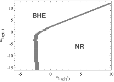
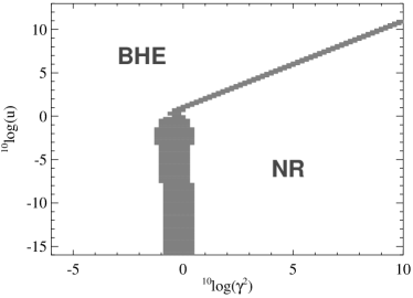
Figure 4: These figures show the source of the Gaunt factor as a function of $\log\gamma^{2}$ and $\log u$ for $Z=1$ (left panel) and $Z=36$ (right panel). The shaded area is where the smooth transition between the BHE and NR data is created.

Figure 5: These figures show the merged free–free Gaunt data for Z=1 as a function of $u$ (left panel) and $\gamma^{2}$ (right panel). Thick curves are labelled with the values of ${}^{10}\log\gamma^{2}$ (left panel) and ${}^{10}\log u$ (right panel) in increments of 5 dex. The thin curves have a spacing of 1 dex.

Figure 6: Same as Fig. 5, but for $Z=36$.

2.3 Spectral simulations with Cloudy

We have incorporated this improved theory into the development version of the spectral simulation code cloudy, which can simulate both photoionised and collisionally ionised gas. The largest differences are expected at high temperatures and photon energies. As an example of the effects of the improved Gaunt factor we show the spectrum of a solar-abundance low-density gas with a temperature of 100 MK in coronal equilibrium in Fig. 7. We compare the old Gaunt data in cloudy version c13.03 (a combination of NR data with various extrapolations) and the new data presented in this paper. The upper panel shows the spectrum while the lower panel shows the ratio of new to old treatments. Significant enhancements in the continuous emission occur at high energies. The new data presented in this paper will be incorporated in the next major release of cloudy.

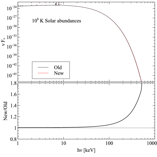
Figure 7: The upper panel shows the spectrum of a 10⁸ K gas with solar abundances in coronal equilibrium, computed both with the old and new treatments. The lower panel shows the ratio. Significant enhancements in the continuous emission are present at high energies.

3 The total free–free Gaunt factor

Similar to paper I, we will include a calculation of the total free–free Gaunt factor which is integrated over frequency. Analytic fits to this quantity were presented in Itoh et al. (2002) for $6.0\leq T_{\rm e}\leq 8.5$ and $1\leq Z\leq 28$. The data presented here extend these results in $T_{\rm e}$ as well as $Z$. The formula for the frequency integrated Gaunt factor is given by Karzas & Latter (1961)

$$\langle g_{\rm ff}(\gamma^{2},Z)\rangle\;=\int_{0}^{\infty}{\rm e}^{-u}\langle g_{\rm ff}(\gamma^{2},u,Z)\rangle{\rm d}u.$$ (4)

The resulting data are shown in Table 2. This quantity is useful for comparing the relativistic and non-relativistic Gaunt factors and assess the magnitude of the relativistic effects as a function of temperature. This comparison is shown in Fig. 8. By inspecting these plots we can see that for $Z=1$ the relativistic effects only become important above $T_{\rm e}=100$ MK. At 100 MK the relativistic effects increase the cooling by slightly more than 0.75% while the magnitude of the effect quickly rises for higher temperatures. At 1 GK the relativistic effects raise the cooling by more than 15%, and at 10 GK by more than 317%. For higher $Z$ species the relativistic effects only become important at higher temperatures than for lower $Z$ species. At $T_{\rm e}=325$ MK the effect is still less than 1% for $Z=36$.

We calculated the total free–free Gaunt factor for all values of $Z$ between 1 and 36. These tables are available in electronic form on the cloudy website. We also provide simple fortran and c programs to interpolate these tables.

Table 2: This table shows an excerpt of the total free-free Gaunt factor as a function of $\gamma^{2}$ for $Z=1$. The full electronic version of this table, as well as tables for other values of $Z$ are available online. Entries 3.92023$+1$ mean $3.92023\times 10^{+1}$

${}^{10}\log\gamma^{2}$	$\langle g_{\rm ff}(\gamma^{2},Z=1)\rangle$
$-6.00$	3.92023$+1$
$-5.90$	3.33120$+1$
$-5.80$	2.82268$+1$
$-5.70$	2.38583$+1$
$-5.60$	2.01184$+1$
$-5.50$	1.69078$+1$
$-5.40$	1.41710$+1$
$-5.30$	1.18333$+1$
$-5.20$	9.85344$+0$
$-5.10$	8.17565$+0$
$-5.00$	6.76918$+0$

Figure 8: The total free–free Gaunt factor as a function of $\gamma^{2}$ and $T_{\rm e}$. The left panel shows a comparison of the merged relativistic data for $Z=1$ (solid line) with the non-relativistic data taken from paper I (dotted line). The right-hand panel shows the same, but for $Z=36$.

4 Summary

In this paper we presented calculations of the relativistic thermally averaged Gaunt factor using the Bethe-Heitler-Elwert approximation. These data are not valid for low temperatures and low photon energies because the Born approximation used by Bethe & Heitler (1934) breaks down in that regime. We have therefore merged our data set with the non-relativistic data we presented in paper I. The BHE approximation is only valid for low values of $Z$, which is why we have restricted our calculations to all values of $Z$ between 1 and 36. A comparison of our calculations with the data presented by N98 showed that they are in good agreement.

We also calculated the frequency integrated Gaunt factor for all values of $Z$ between 1 and 36. We compared these calculations with the non-relativistic total Gaunt factor presented in paper I. From this comparison we concluded that relativistic effects only become important for electron temperatures in excess of 100 MK and that relativistic effects are less pronounced for higher $Z$ species at the same temperature.

All data presented in this paper are available in electronic form from MNRAS as well as the cloudy website at http://data.nublado.org/gauntff/. In addition to these data tables, we also present simple interpolation routines written in fortran and c on the cloudy website. They use a 3rd-order Lagrange scheme to interpolate the logarithm of the thermally averaged Gaunt data. This reaches a relative error better than $3\times 10^{-3}$ everywhere. The next release of cloudy will contain a vectorised version of the interpolation routine which is faster, while maintaining the same precision. It is based on the Newton interpolation technique. The program used to calculate all data is also available from the cloudy website.

References

- Bethe & Heitler (1934) Bethe H., Heitler W., 1934, Royal Society of London Proceedings Series A, 146, 83
- Elwert (1939) Elwert G., 1939, Annalen der Physik, 426, 178
- Elwert & Haug (1969) Elwert G., Haug E., 1969, Physical Review, 183, 90
- Ferland et al. (2013) Ferland G. J., Porter R. L., van Hoof P. A. M., Williams R. J. R., Abel N. P., Lykins M. L., Shaw G., Henney W. J., Stancil P. C., 2013, Rev. Mex. Astron. Astrofis., 49, 137
- Gaunt (1930) Gaunt J. A., 1930, Phil. Trans. R. Soc. A, 229, 163
- Itoh et al. (1985) Itoh N., Nakagawa M., Kohyama Y., 1985, ApJ, 294, 17
- Itoh et al. (2002) Itoh N., Sakamoto T., Kusano S., Kawana Y., Nozawa S., 2002, A&A, 382, 722
- Itoh et al. (2000) Itoh N., Sakamoto T., Kusano S., Nozawa S., Kohyama Y., 2000, ApJS, 128, 125
- Karzas & Latter (1961) Karzas W. J., Latter R., 1961, ApJS, 6, 167
- Nozawa et al. (1998) Nozawa S., Itoh N., Kohyama Y., 1998, ApJ, 507, 530 (N98)
- Pratt & Tseng (1975) Pratt R. H., Tseng H. K., 1975, Phys. Rev. A, 11, 1797
- van Hoof et al. (2014) van Hoof P. A. M., Williams R. J. R., Volk K., Chatzikos M., Ferland G. J., Lykins M., Porter R. L., Wang Y., 2014, MNRAS, 444, 420 (paper I)