Single pulse and profile variability study of PSR J1022+1001

Abstract

Millisecond pulsars (MSPs) are known as highly stable celestial clocks. Nevertheless, recent studies have revealed the unstable nature of their integrated pulse profiles, which may limit the achievable pulsar timing precision. In this paper, we present a case study on the pulse profile variability of PSR J1022+1001. We have detected approximately 14,000 sub-pulses (components of single pulses) in 35-hr long observations, mostly located at the trailing component of the integrated profile. Their flux densities and fractional polarisation suggest that they represent the bright end of the energy distribution in ordinary emission mode and are not giant pulses. The occurrence of sub-pulses from the leading and trailing components of the integrated profile is shown to be correlated. For sub-pulses from the latter, a preferred pulse width of approximately 0.25 ms has been found. Using simultaneous observations from the Effelsberg 100-m telescope and the Westerbork Synthesis Radio Telescope, we have found that the integrated profile varies on a timescale of a few tens of minutes. We show that improper polarisation calibration and diffractive scintillation cannot be the sole reason for the observed instability. In addition, we demonstrate that timing residuals generated from averages of the detected sub-pulses are dominated by phase jitter, and place an upper limit of $\sim 700$ ns for jitter noise based on continuous 1-min integrations.

1 Introduction

Rotation-powered pulsars have been shown to be stable celestial clocks (e.g. Verbiest et al., 2009) and thus excellent tools in the ongoing endeavours of high precision gravity tests (Kramer et al., 2006), neutron star equations of state (Demorest et al., 2010; Özel et al., 2010), and gravitational wave detection (van Haasteren et al., 2011; Yardley et al., 2011; Demorest et al., 2013; Shannon et al., 2013). These experiments utilise the high precision timing of millisecond pulsars (MSPs), which are known for their rotational stability and the stability of their integrated pulse profiles (which do not change over many years). However, recent studies have shown that the profiles of MSPs can exhibit low-level instabilities that may limit the achievable timing precision. In general, these instabilities can be categorized into two types: temporally uncorrelated variabilities caused by the instability of single pulses (e.g. Jenet et al., 1998; Liu et al., 2012; Shannon & Cordes, 2012), and temporally correlated variations induced by other phenomena (e.g. Kramer et al., 1999; Edwards & Stappers, 2003a). The contribution of jitter to the pulsar timing noise could be mitigated by simply increasing the exposure time or by correcting the biased integrated profiles with suitable algorithms (Cordes & Shannon, 2010; Osłowski et al., 2013). Comprehensive studies of profile instabilities would give new insights into the fundamental timing limits and thereby potentially improving the timing precision, which is essential for the aforementioned astrophysical experiments.

PSR J1022+1001 is a MSP with a rotation period of approximately 16 ms. It exhibits a regular rotational behaviour and is included in the current pulsar timing array observations for the purpose of gravitational wave detection (e.g. Manchester, 2013). The pulsar is in a binary with a 7.8-day orbital period with a white dwarf companion, and is thus a potential laboratory for testing the Strong Equivalence Principle (e.g. Freire et al., 2012; Antoniadis et al., 2013). The integrated pulsed profile of the pulsar consists of a double-peaked structure at L-band frequencies with a highly linearly polarised trailing component. The amplitude ratio of the two components has been shown to change significantly as a function of frequency (Ramachandran & Kramer, 2003). There is also evidence that the ratio is unstable across time and may even evolve on short timescales of tens of minutes (Kramer et al., 1999; Purver, 2010). Meanwhile, as the trailing component of the pulse profile is highly polarised, profile instability could also arise from improper polarisation calibration due to an imperfect receiver model (Hotan et al., 2004). A better understanding of the profile variation in this system is therefore essential in order to further improve the timing precision of PSR J1022+1001. This may be used to assess and perhaps correct for profile variations in other MSPs.

Examining single pulses has not been common in MSPs owing to their typically lower flux densities compared to normal pulsars. Exceptions are the so-called giant pulses which have been detected only in a few bright MSPs (e.g. Cognard et al., 1996; Romani & Johnston, 2001; Joshi et al., 2004; Knight et al., 2005). Analysis of the weak single pulses has been only carried out in the few brightest MSPs (Jenet et al., 1998; Jenet et al., 2001; Edwards & Stappers, 2003a; Shannon & Cordes, 2012; Osłowski et al., 2014). Based on an autocorrelation analysis, Edwards & Stappers (2003a) have shown evidence for pulse intensity modulation at the phase of the trailing component in PSR J1022+1001. However, no detailed investigation into the single pulses has been undertaken so far, due to either limited system sensitivity or the lack of high-resolution instrumentation.

The rest of this paper is structured as follows: In Section 2 we describe the details of observations and data processing. Results of the detected single pulses, integrated profile stability, and timing analysis are presented in Section 3. We conclude and discuss the results in Section 4.

2 Observation

Simultaneous observations of 7 to 9 hours in duration of PSR J1022+1001 were conducted with the Westerbork Synthesis Radio Telescope (WSRT) and the Effelsberg 100-m Radio Telescope, at four epochs. A summary of the observations can be found in Table 1. The two telescopes were chosen as they provide similar sensitivities at L-band so that profile instability could be verified from both sites at the same time. In addition, Effelsberg is an alt-azimuth telescope, meaning that it tracks a source across the sky, the changing parallactic angle (PA) results in varied Stokes parameters which need to be properly calibrated. On the other hand, the WSRT is equatorially mounted with no PA variation and thus in principle not influenced by this effect. Therefore, using data from these two telescopes allows us to cross-check the result of polarisation calibration which was claimed to be the main cause of profile instability (Hotan et al., 2004; van Straten, 2013).

Table 1: Parameters of the simultaneous observations of PSR J1022+1001 with the WSRT and the Effelsberg 100-m Radio Telescope. The symbols $T$, $f_{\rm o}$, and $\Delta t_{\rm s}$ represent the duration of observation, overlapping observing frequency range, and the single pulse time resolution at the WSRT.

MJD	$T$ (hr)	$f_{\rm o}$ (MHz)	$\Delta t_{\rm s}$ ($\mu$s)
55909	7.0	1300-1440	4.0
55974⋆	8.4	1300-1440	4.0
56158	8.5	1300-1440	2.0
56257	9.0	1300-1365∗	2.0

^⋆At this epoch the Effelsberg data were corrupted due to a problem with the signal attenuators (see Appendix A for more details).
^∗At this epoch three 25 MHz sub-bands of Effelsberg data were lost due to hard drive failure.

At the WSRT we used the PuMa-II system to record 8-bit baseband data (Karuppusamy et al., 2008), which were later processed offline in two stages. In the first stages the 8$\times$20 MHz bands were combined to form a multi-band data stream corresponding to a 160 MHz contiguous band centered at 1380 MHz, at the original time resolution of 25 ns. The DSPSR software (for details see van Straten & Bailes, 2011) was used to coherently dedisperse the data over the entire bandwidth using a 64-channel synthetic software filterbank at the DM of 10.246 cm^-3pc and folded to form 10-s averages in the second stage. Additionally, we searched for significant single pulses at this stage. This was done after summing up the total intensities of all frequencies, and averaging by the number of frequency channels. Any pulse period that contained a peak greater than five times the root-mean-square (rms) of the off-pulse noise was written out as a single pulse candidate. In the post-processing stage, these were then confirmed to be true pulses by comparing the phase to that of the integrated pulse profile.

At Effelsberg, the new PSRIX pulsar backend (Karuppusamy et al., in prep) was used in baseband mode. These data were reduced in the same way as the WSRT data, except that here, 8$\times$25 MHz bands were produced with a central frequency of 1347.5 MHz. In addition, at regular intervals of 40 min, the telescope was pointed $0.5^{\circ}$ off-source for 90 s, when a pulsed noise signal was injected at $45^{\circ}$ into the feed probes as a calibrator for polarimetry.

The 10-s integrations and single pulses were then processed with the psrchive software package (Hotan et al., 2004). For the 10-s integrations from Effelsberg we performed polarisation calibration with the single-axis receiver model which corrects for the differential gains between the two feeds. Next we used pazi (psrchive’s interactive RFI zapper) to clean the radio frequency interference (RFI) by visual examination of the averaged pulse profiles and single pulse candidates. Finally, we selected all 10-s integrations that overlapped in time between the two telescopes, and then removed the non-overlapping frequency channels, leading to an overlapping observing frequency range of $1300-1440$ MHz.

Example polarisation profiles of PSR J1022+1001 from both the WSRT and the Effelsberg observation at MJD 56257 centred at 1320 MHz, can be found in Fig. 1. The integrated profile shows a double-peaked structure, with the trailing component consisting of highly linearly polarised emission. The polarisation properties are in agreement between the two sites, with a correlation coefficient of 0.999 (as defined in Liu et al., 2012). Given the profile instability of this pulsar, especially in observations separated by several years (Purver, 2010), the polarisation components qualitatively agree with the previous observations (Kramer et al., 1999; Ramachandran & Kramer, 2003; van Straten, 2013).

Figure 1: Polarisation profiles of PSR J1022+1001 obtained at MJD 56257 from the Effelsberg (middle) and the WSRT (bottom) observation at 1.3 GHz. The P.A. in the top panel stands for the polarisation position angle of the linear component. The Effelsberg and the WSRT data show consistent P.A. curves and here we plot the one from the Effelsberg data as a demonstration. The solid, dashed and dotted lines represent the Stokes parameters $I$, $L$ and $V$, respectively. There is a “negative” dip, i.e., an underestimation of system temperature, on the WSRT total intensity profile (at phase 0.52) which corresponds to the low-bit sampling artefact discussed in Jenet & Anderson (1998). This is due to the fact that the signal was originally quantized using 2 bits per sample at each individual dish of the WSRT. Further investigation shows that the dip is mostly from high frequency channels within each 20 MHz band. The total intensity profile is slightly lowered by this underestimation, which makes the valley region between the two components appear over polarised. Further investigations can be found in Appendix A.

3 Results

3.1 Sub-pulse properties

In a total of 35 hours of observations, we have approximately 14,400 single pulse detections above our 5-$\sigma$ threshold, which corresponds to about 700 sub-pulses located at the leading component of the integrated profile and about 13,700 at the trailing component. The detections were all made from the observations at MJD 55909 and 56257 as the pulsar was significantly weaker due to interstellar scintillation at MJD 55974 and 56158. The highest peak signal-to-noise ratio of detection is close to 10. Fig. 2 shows the sub-pulse detections achieved at MJD 56257 at their occurrence epochs and peak signal-to-noise ratios (S/N_s) relative to the local average S/N of all single pulses observed during the 5-min interval centred at the epoch of the single pulse ($\langle{\rm S/N}_{\rm s}\rangle_{\rm 5min}$). We can see that there is an evolution in the ratio which is due to the pulsar flux decreasing because of interstellar scintillation. With our sensitivity, useful detections are feasible only when integrating 5-min observations results in a profile of peak S/N (S/N_5min) above 30. The detection rate is highest between MJD 56257.055 and 56257.060, corresponding to 4.5% of all rotations. We have calculated time separations between neighbouring sub-pulses at the trailing component within this period of time, and over 95% of them are less than 1 s, indicating that pulse nulling with duration longer than 1 s ($\simeq 60$ rotations) is not detected.

Figure 2: Sub-pulses detected at MJD 56257 as a function of time and their peak signal-to-noise ratios (S/N_s) divided by the local average S/N of all single pulses observed during the 5-min interval centred on the epoch of the single pulse ($\langle{\rm S/N}_{\rm s}\rangle_{\rm 5min}$). The location of peak bin was selected based on a 16-$\mu$s time resolution. The top panel shows detections at the phase of the leading component in the averaged profile, and the bottom shows those at the phase of the trailing one.

Fig. 3 shows the distribution of the peak amplitude phases for the detected sub-pulses, compared with the integrated profile. All detections were obtained within the on-pulse phase and most of them are clustered within the range defined by the trailing component in the average profile. The two maxima correspond to the two peaks in the phase-resolved modulation index of Edwards & Stappers (2003b). In Fig. 4 we plot the distribution of the flux densities of the sub-pulses divided by the averaged flux densities of a single pulse in 5-min integrations. The plot demonstrates that none of the detections has a flux density that is above 3.8 times the average, and there is therefore no evidence for giant pulses.

Figure 3: Distribution of peak amplitude phase for all detected sub-pulses (lower panel), in comparison with the integrated profile (upper panel). Again, the peak bins were chosen based on a 16-$\mu$s time resolution. The integrated profile is from the WSRT observation at MJD 56257.

Figure 4: Distributions of relative flux densities to averaged single pulse flux densities in 5-min integrations, for sub-pulses detected at the leading and trailing components, respectively. No pulse with flux above 3.8 times the average has been seen.

Fig. 5 presents example polarisation profiles of sub-pulses at the phase of the leading and trailing components. It can be seen that pulses from the leading component do not show significant polarisation, while those from the trailing component are highly linearly polarised. The polarisation fractions of both components are consistent with the integrated pulse profile, suggesting that the detected sub-pulses represent the bright end of the energy distribution of all pulses. The bottom plot in Fig. 5 shows the averages of the leading and trailing component pulses, respectively, whose polarisation characteristics are in agreement with the corresponding individual detections. It is interesting to note that in both averages, the components that do not include detected sub-pulses are consistent with the average of all periods in total intensity. This means that during the occurrence of bright emission in one component, there still exists emission at an average level at the location of the other component.

Figure 5: Example polarisation profiles of sub-pulses detected at MJD 56257, at the phase of the leading (top) and trailing (middle) component in the average profile. The bottom plot shows the integrations of detected sub-pulses from the leading (upper panel) and trailing (lower panel) components, respectively. The solid, dashed and dotted lines stand for the Stokes $I$, $L$ and $V$, respectively. The dashed-dotted line represents the averaged total intensity of all periods.

Meanwhile, sub-pulses can be detected from the leading and trailing components within the same pulse period. In total, about 280 such events have been detected. In all events, the two phases of peak amplitude are well separated from the phase bound 0.485 (used to group the detections), excluding detections of a single pulse with broad width spreading over the region of both components. We will later refer to such an event as a ‘bi-pulse’, and their corresponding integrated profile is shown in Fig. 6. The valley region between the two components is significantly steeper in this profile than the ordinary average in Fig. 1, while the polarisation properties of the two components are consistent. To investigate the correlation of occurrence between the leading and trailing component pulses, we carried out a further statistical study. Pulses were selected at both epochs, from the period of time when the leading component pulses could be detected. A summary of the selections can be found in Table 2. We formed the statistical test problem in the following statement:

$$\left\{\begin{array}[]{l l}H_{0}&\textrm{Leading and trailing pulses are uncorrelated.}\\ H_{1}&\textrm{Leading and trailing pulses are correlated.}\end{array}\right.$$

The bi-pulse phenomenon is defined as: both the leading and trailing component pulses are detected within a single period. Thus, under the null-hypothesis $H_{0}$, in each pulse period the probability of observing bi-pulses is

$$P_{\rm b}=P_{\rm l}P_{\rm t}\,,$$ (1)

where $P_{\rm b},P_{\rm l}$ and $P_{\rm t}$ are the probabilities of observing bi, leading, and trailing component pulses, respectively. By combining the statistics from these two epochs, we have calculated the observed $P_{\rm l}$ and $P_{\rm t}$ which gives an expected value of $P_{\rm b}$ as $3.80\pm 0.16\times 10^{-5}$ under the null-hypothesis $H_{0}$. Meanwhile, the observed bi-pulse occurrence probability was calculated to be $6.32\pm 0.39\times 10^{-4}$, about 17 times larger. For a more quantitative study, over $N$ pulse periods the statistical distribution function $f$ of the total number of bi-pulses, leading and trailing component pulses are

$$f(N_{\rm b}|P_{\rm b},N)=C_{N}^{N_{\rm b}}P_{\rm b}^{N_{\rm b}}(1-P_{\rm b})^{N-N_{\rm b}}\,,$$ (2)

$$f(N_{\rm l}|P_{\rm l},N)=C_{N}^{N_{\rm l}}P_{\rm l}^{N_{\rm l}}(1-P_{\rm l})^{N-N_{\rm l}}\,,$$ (3)

$$f(N_{\rm t}|P_{\rm t},N)=C_{N}^{N_{\rm t}}P_{\rm t}^{N_{\rm t}}(1-P_{\rm t})^{N-N_{\rm t}}\,,$$ (4)

where $C_{b}^{a}$ is the binomial coefficient defined as $C_{b}^{a}=(b!)/(a!(b-a)!)$. Using the Bayesian theorem with a flat prior for the distributions of probability of each type of pulses, we have

$$f(P_{\rm l}|N_{\rm l},N)=f(N_{\rm l}|P_{\rm l},N)(N+1)\,,$$ (5)

$$f(P_{\rm t}|N_{\rm t},N)=f(N_{\rm t}|P_{\rm t},N)(N+1)\,,$$ (6)

where $f(P_{\rm l}|N_{\rm l},N)$ and $f(P_{\rm t}|N_{\rm t},N)$ are the posterior for $P_{\rm l}$ and $P_{\rm t}$. Thus the probability distribution of $N_{\rm b}$ given $N_{\rm l}$ and $N_{\rm t}$ is

$$f(N_{\rm b}|N_{\rm l},N_{\rm t},N) = \int_{0}^{1}\int_{0}^{1}dP_{\rm l}dP_{\rm t}C_{N}^{N_{\rm b}}(P_{\rm l}P_{\rm t})^{N_{\rm b}}$$ (7)

$$(1-P_{\rm l}P_{\rm t})^{N-N_{\rm b}}$$

$$f(P_{\rm l}|N_{\rm l},N)f(P_{\rm t}|N_{\rm t},N)\,.$$

Under the null hypothesis $H_{0}$, we have

$$P(N_{\rm b}>N_{\rm B}\textrm{ or }N_{\rm b}<N_{\rm A})=1-\sum_{N_{\rm A}}^{N_{\rm B}}f(N_{\rm b}|N_{\rm l},N_{\rm t},N)\,,$$ (8)

where $P(N_{\rm b}>N_{\rm B}~{}\textrm{or}~{}N_{\rm b}<N_{\rm A})$ is the probability of finding that the occurrence of bi-pulses $N_{\rm b}$ is greater than the threshold $N_{\rm B}$ or less than the threshold $N_{\rm A}$, under the assumption that the leading and trailing component pulses are uncorrelated. This provides a good statistic for testing whether the observations agree with the null hypothesis $H_{0}$. Accordingly, we have estimated the probability to detect more than $N_{\rm b}$ bi-pulses ($P(n>=N_{b})$) based on the statistics in Table 2, which appears to be very close to zero at both epochs. We therefore conclude that the leading and trailing component pulses are correlated in their occurrence, otherwise it would be extremely rare to observe such a high value of $N_{\rm b}$ with the null-hypothesis $H_{0}$. In young pulsars, correlated emission modulation at different rotational phases has been found in a few cases (Weltevrede et al., 2012, Karuppusamy et al. in prep.).

Figure 6: Polarisation profile averaged over all detected bi-pulses, where sub-pulses were detected at both components within a single period.

Table 2: Summary of selected pulses used to investigate the occurrence correlation between the leading and trailing component pulses. Here N, N_l, N_t and N_b denote the number of periods within the time range the pulses were chosen from, number of leading and trailing component pulses, and number of bi-pulses, respectively. The probability of detecting more than $N_{\rm b}$ bi-pulses is denoted by $P(n\geqslant N_{b})$

. Phase MJD 55909 MJD 56257 N $2.1\times 10^{5}$ $2.0\times 10^{5}$ N_l 72 525 N_t 2737 7929 N_b 25 234 $P(n>=N_{b})^{\ast}$ $10^{-252}$ $10^{-881}$
^∗ Due to the difficulties in the numerical evaluation of the integral, we used asymptotic values for the error function. This could result in one order of magnitude error, but will not change the conclusion.

Jenet et al. (1998) showed an inverse correlation between pulse width and peak amplitude for the sub-pulses of PSR J0437$-$4715. In Fig. 7 we perform the same investigation by showing the distribution of detected pulses from the trailing component on a width$-$relative S/N_s plane. Here, to avoid bias caused by a variable detection threshold, we only selected detections between MJD 56257.042 and 56257.066 and with $({\rm S/N}_{\rm s})/(\langle{\rm S/N}_{\rm s}\rangle_{\rm 5min})>7$. It is interesting to note that, instead of an anti-correlation, there exists a favoured pulse width value of about 0.25 ms which is consistent for pulses of different relative S/N_s values. The probability of occurrence also does not favour pulses with narrow width and high peak amplitude. Fig. 8 gives the distribution of the same pulses with respect to their phases and relative S/N_s. The plot demonstrates that the occurrence phases of the sub-pulses are strongly clustered, especially for those of peak 10 times above average. The phenomenon that brighter pulses show up earlier in phase, found for PSR J1713+0747 in Shannon & Cordes (2012), is not seen. The property of regular shape and phase could possibly be translated into precise pulse time-of-arrival (TOA) measurements, which will be further investigated in Section 3.3.

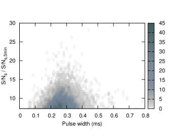
Figure 7: Distribution of pulses from the trailing component by their relative S/N_s and width. To avoid bias caused by the time-variant detection threshold, only pulses with epoch between MJD 56257.042 and 56257.066, and $({\rm S/N}_{\rm p})/(\langle{\rm S/N}_{\rm s}\rangle_{\rm 5min})>7$, were selected. Again, the peak bins were selected based on a 16-$\mu$s time resolution.

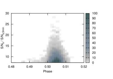
Figure 8: Distribution of the same pulses as in Fig. 7 on a phase$-$relative S/N_s plane.

3.2 Variation of integrated profiles and sub-pulse occurrence

As mentioned in Section 1, it has not been conclusively shown whether the average profiles of PSR J1022+1001 exhibit intrinsic shape variation. Here, following the idea of previous analyses (e.g. Kramer et al., 1999), we calculate the amplitude ratio of the leading and trailing components of total intensity profiles for 10-min integrations, and plot them against time. For each component, the amplitudes were defined as the total intensity within a fixed phase range (1.7% of a period), after subtracting the baseline. Their errors were calculated from the rms of the off-pulse bins. We used a 40 MHz sub-band ranging from 1300 to 1340 MHz, where for most of our observing time, the flux density is the highest within the entire overlapping band. The results from data at MJD 55909 and 56257 are shown in Fig. 9, where at both epochs the measurements show a clear evolution with time and are consistent between the two sites. The variation trend is similar to what has been indicated in Fig. 3.6 of Purver (2010). We also calculated the weighted correlation coefficients ( $\rho_{\rm w}$s) between trends from the two sites, which is defined as

$$\rho_{\rm w}=\frac{{\rm cov}_{\rm w}(\mathcal{E}_{i},\mathcal{W}_{i},\sigma_{\mathcal{E},i},\sigma_{\mathcal{W},i})}{\sqrt{{\rm cov}_{\rm w}(\mathcal{E}_{i},\mathcal{E}_{i},\sigma_{\mathcal{E},i},\sigma_{\mathcal{E},i}){\rm cov}_{\rm w}(\mathcal{W}_{i},\mathcal{W}_{i},\sigma_{\mathcal{W},i},\sigma_{\mathcal{W},i})}}.$$ (9)

Here $\mathcal{E}_{i}$, $\mathcal{W}_{i}$ are the ratio measurements from Effelsberg and WSRT, respectively, $\sigma_{\mathcal{E},i}$, $\sigma_{\mathcal{W},i}$ are their measurement errors, and ${\rm cov}_{\rm w}$ is the weighted covariance defined by

$${\rm cov}_{\rm w}(x_{i},y_{i},\sigma_{x,i},\sigma_{y,i})=\frac{\displaystyle\sum_{i}(x_{i}-\overline{x})(y_{i}-\overline{y})/(\sigma^{2}_{x,i}\sigma^{2}_{y,i})}{\displaystyle\sum_{i}1/(\sigma^{2}_{x,i}\sigma^{2}_{y,i})},$$ (10)

where the overline stands for weighted mean. The calculated $\rho_{\rm w}$ is 0.60 at MJD 55909 and 0.91 at MJD 56257, respectively, confirming that measurements from the two sites exhibit the same evolution trend. Note that at the beginning of MJD 56257 the pulsar was significantly brighter and the profile was showing a steeper variation trend than at MJD 55909, which thus corresponds to a value of $\rho_{\rm w}$ closer to unity. To understand the estimation error of $\rho_{\rm w}$, we performed a Monte Carlo simulation. In each iteration, we randomly altered the measured component amplitudes based on Gaussian distributions with the standard deviation equal to the measurement errors, and thus calculated a new amplitude ratio and $\rho_{\rm w}$. Fig. 10 shows the histogram of $\rho_{\rm w}$ with 10,000 iterations obtained from measurements at MJD 56257, where $\rho_{\rm w}$ is larger than 0.78 and 0.64, with 68% and 95% confidence level, respectively. The same investigation has also been performed for the measurements at MJD 55909 and the corresponding thresholds are 0.40 and 0.20, respectively. These mostly rule out the possibility of a non-correlation between the two sites. A brief summary of the results can be found in Table 3.

Figure 9: Amplitude ratio measurements of the two components in the PSR J1022+1001 total intensity profiles from two epochs. The measurements were made using 10-min integrations of a 40 MHz band centred at 1320 MHz. Note that measurements of fractional error larger than 10% were discarded, which leads to the gap within the results at MJD 56257.

Figure 10: Distribution of $10^{4}$ simulated values of $\rho_{\rm w}$ based on amplitude ratio measurements from data obtained at MJD 56257.

Table 3: Weighted correlation coefficient ($\rho_{\rm w}$) between the amplitude ratio measurements from the WSRT and Effelsberg data at two epochs, as well as their lower limits with 68% ($\mathcal{L}_{68}$) and 95% ($\mathcal{L}_{95}$) confidence level.

MJD	$\rho_{\rm w}$	$\mathcal{L}_{68}$	$\mathcal{L}_{95}$
55909	0.60	0.40	0.20
56257	0.91	0.78	0.64

To investigate the effect of polarisation calibration on our results, we also applied the template-matching calibration technique to the Effelsberg data at MJD 55909 and 56257 (van Straten, 2006, Lee et al. in prep.), based on the template polarisation profile from European Pulsar Network Pulse Profile Database (Stairs et al., 1999) showing consistent polarimetry with previous published results. For this calibration scheme, we used both the single-axis and the reception description of the receiver properties, the latter of which models both the differential gain and cross-coupling of the two feeds (Ord et al., 2004; van Straten, 2004). The calibrated data were then processed by following the same procedure as described above. Both receiver models led to a fit with reduced $\chi^{2}$ close to unity. Still, the effect of feed cross-coupling was estimated to influence the total intensity profile by less than 1%, and the true value could not be measured due to limited sensitivity. As a demonstration, in Fig. 11 we show the obtained polarisation profiles from MJD 56257 data with the calibration result based on calibrators and the single-axis model shown in Fig. 1. It can be seen that the three profiles from different calibration schemes or models exhibit consistent polarisation properties, especially the two achieved with the single-axis model. Using the reception model results in a slightly lower linear polarisation percentage (middle panel), mostly due to absorption of power into the feed leakage terms. In addition, the calculated $\rho_{\rm w}$s between the new amplitude ratio measurement trend and the WSRT result, is 0.89 when using the reception model and 0.91 when single-axis calibration was applied. These are almost the same as the value obtained above. The same analysis at MJD 55909 data led to $\rho_{\rm w}=0.55$ when using the reception model and $\rho_{\rm w}=0.60$ when applying single-axis calibration, also consistent with the result based on calibrators. Further investigation based on independent Effelsberg data for the Large European Array for Pulsars project (Kramer & Stappers, 2010), shows that the circular receiver does not suffer from strong cross-coupling between the two feeds (Lee et al. in prep.), which validates the use of the single-axis model in this case. Therefore, it is highly unlikely that our detected profile variation is due in large part to improper polarisation calibration.

Figure 11: Comparison of Effelsberg polarisation profiles obtained from data at MJD 56257, based on calibrator+single-axis model (left), template+reception model (middle), and template+single-axis model (right). The solid, dashed and dotted lines stand for the Stokes parameter $I$, $L$ and $V$, respectively.

Figure 12: Measured amplitude ratios as a function of frequency, from the profile models obtained at MJD 55909. The measurements from the Effelsberg and WSRT data are based on profiles of bandwidth 6.25 and 5 MHz, respectively. The edges of the 20 MHz sub-bands (starting from 1300 MHz) in the WSRT data have been marked by dashed lines. Note that for the WSRT data there is an additional increase of the measurement values within a sub-band, associated with the low-bit digitisation artefact shown in Fig. 1. More details of this effect are shown in Appendix A.

Note that the profile shape has a clear frequency dependence (e.g. Ramachandran & Kramer, 2003). If the flux density distribution within the observing band changes significantly in time due to ISM diffractive scintillation, the averaged profiles (after frequency summation) may therefore also exhibit time-variant behaviour (e.g. Liu et al., 2011). To understand its contribution to our results, here we simulate the varying trends by this effect and compare them with the real measurements. At each epoch, we first used an integrated profile for the entire duration of the observation to establish a profile model with frequency dependent shape. As an example, Fig. 12 shows the measured amplitude ratios as a function of frequency from the profile models for the MJD 55909 data. We then applied the measured frequency-dependent flux densities from each 10-min integration to the model to create a simulated profile, and computed the resulting amplitude ratio after frequency summation. For this purpose, we kept the frequency resolution of 6.25 MHz for the Effelsberg data and 10 MHz for the WSRT data, so as to have enough signal within each frequency channel. The channel width is significantly smaller than the estimated scintillation bandwidth of this pulsar (Cordes & Lazio, 2002; You et al., 2007). The uncertainties in the amplitude ratios of the simulated profiles were calculated from the measurement errors of the flux densities estimated from each frequency channel of each 10-min integration. The flux densities as well as their errors were measured by using pdv (psrchive’s archive data displayer), where the flux density is defined as the total intensity within a pulse period after subtracting the baseline, and their errors were calculated from the rms of off-pulse phase bins defined by 3-$\sigma$ threshold. By following this procedure, the observed variation trend would be reproduced if the profile instability is mostly dominated by the scintillation effect. In Fig. 13 we present the results at MJD 55909 and 56257 from both sites, based on both the selected 40 MHz sub-band and the entire bandwidth. Clearly, in most cases the simulation resulted in a flat trend and did not reproduce the actual measurements. The reduced $\chi^{2}$s of the measurement series with respects to their corresponding simulated trend fell in between 2.0 and 22, all significantly above unity. We therefore conclude that our detected profile instability shown in Fig. 9 is not significantly affected by the scintillation effect.

Figure 13: Simulated peak amplitude ratios based on flux densities measured from 10-min integrations, compared with the actual ratio measurements. The simulations were carried out on both the WSRT (left) and Effelsberg (right) data at MJD 55909 (top) and 56257 (bottom), using both the 40 MHz sub-band and the entire available bandwidth. The uncertainties of the simulated ratios are typically of order $\lesssim 10^{-3}$, and thus not visible from plots. Note that for MJD 56257, the analysis was carried out only for the first half of the data, as in the second half the flux densities within individual frequency channels were not measurable on many occasions due to low S/Ns. The effective observing bandwidth of Effelsberg at MJD 55909 is 160 MHz due to a receiver cutoff below 1280 MHz.

We do not detect profile variation at the other two epochs, MJD 55974 and 56158, mostly because the source was comparatively dim due to scintillation. At these two epochs, with the WSRT 160 MHz observations the S/N_5min values are all below 30, while the maxima at MJD 55909 and 56257 reach 75 and 110, respectively. This may explain the contradictory conclusions from previous studies on profile stability on short timescales. In addition, it can be seen from Fig. 9 that the amplitude ratio variation may not be significant enough for detection within 0.1 day, which is the longest observation used in previous work. Therefore, detection of profile instability is achievable only when the pulsar is bright and the variation is large.

We note that our analysis draws seemingly different conclusions on the profile stability of PSR J1022+1001 compared to Liu et al. (2012), due to a few reasons. Firstly, our new observations detected the pulsar when it was significantly brighter than in the previous ones. For instance, at the beginning of the MJD 56257 observation an integration time of 1800 s led to a profile with signal-to-noise ratio over 800, while integrating the entire observation (approximately 1,900 s) in Liu et al. (2012) only resulted in a value of about 480. Secondly, the work in Liu et al. (2012) was based on 1-min integrations and thus focused more on searching for random variations in profile shapes on short timescales. Finally, the duration of the previous observation does not provide the sensitivity to profile variations on a timescale of several tens of minutes detected in this paper.

In principle, the profile variation can be fully attributed to the detected bright sub-pulses, if either their shape or occurrence rate varies by a sufficiently large amount in time. Such a possibility has been investigated in Fig. 14. To balance between potential shape bias introduced by a variable detection threshold and time span allowing us to see profile variation, here we selected sub-pulses detected with $({\rm S/N}_{\rm s})/(\langle{\rm S/N}_{\rm s}\rangle_{\rm 5min})>9$ and MJD between 56257.042 and 56257.074. It can be seen that while the amplitude ratios from 5-min integrations is gradually increased in time ($\approx 6$% from MJD 56257.04 to 56257.07), no similar variation trend is witnessed from the averages of the sub-pulses. This indicates that the profile variation is not caused by the selected bright sub-pulses. In fact, the number of detected sub-pulses is approximately $200-300$ per 5-min window ($1-1.5\%$ of all periods). Therefore, the amplitude ratios of the sub-pulse averages would need to change by a factor of 4 or more if variability in the $1-1.5\%$ of detected sub-pulses were the cause of the profile variation in 5-min integrations. Note that the number of detected sub-pulses remain consistent in time, though it is proportional to the S/N of 5-min integrations, which is expected due to variability in detection sensitivity. This suggests that the profile variation is not induced by the occurrence rate variation of bright sub-pulses. In fact, assuming profile variation mainly occurs at the trailing component, the increase of amplitude ratio from 5-min integrations corresponds to 6% decrease of the flux density at the trailing component. Given the average amplitude ratio of 0.18 observed in the detected sub-pulses and an amplitude ratio of 1 for ordinary integrations, the selected sub-pulses contribute 6-9% of the flux density at the trailing component. Therefore, if the change of occurrence rate of the selected sub-pulses were fully responsible for the amplitude ratio variation, the number of detections around MJD 56257.07 would have dropped by 70-100%, which is clearly not the case. Therefore, it is unlikely that our selected sub-pulses cause the detected profile variation, which suggests that sub-pulse variability and integrated profile variation are two different effects. Nevertheless, the analysis is still restricted to roughly the brightest 1% of all single pulses, and will be significantly improved by increasing system sensitivity.

Figure 14: Top to bottom: amplitude ratio measurements from 5-min integrations and from sub-pulse averages, numbers of sub-pulses in 5-min, S/Ns of 5-min integrations. Here the sub-pulses were selected with $({\rm S/N}_{\rm s})/(\langle{\rm S/N}_{\rm s}\rangle_{\rm 5min})>9$ and MJD between 56257.042 and 56257.074. The 5-min integrations were formed from WSRT data.

3.3 Timing of sub-pulses

To investigate the impact of sub-pulses on pulsar timing, we used the sub-pulses selected in Fig. 7 (3.4% of all periods, from the trailing component, in total approximately 4,500 pulses) and compared their timing with ordinary integrations based on all rotations. The TOAs are measured by following the classic template-matching method described in Taylor (1992). The template profile for timing based on sub-pulses is formed by summing all detected sub-pulses and performing a Gaussian component smoothing as in e.g. Kramer (1994). The timing residuals were calculated with the TEMPO2 software package (Hobbs et al., 2006). Here we used the timing solution obtained from the European Pulsar Timing Array collaboration (Desvignes et al. in prep.), without fitting for any parameters.

In Fig. 15 we present the timing residuals calculated with averages of 30 pulses (not contiguous in time), equivalent to an integration time of 0.5 s. The timing solution has an rms of 4.3 $\mu$s which is greater than the average of the errors owing to white noise (1.6 $\mu$s). This suggests the existence of phase jitter. To better understand the timing noise, a standard Kolmogorov-Smirnov (K-S) test has been performed on the TOAs as done in Liu et al. (2012). The measured p-value ($\simeq 0.98$) is close to 1, indicating no significant deviation of the residuals from a Gaussian distribution (e.g. Press et al., 1986). In Fig. 16 we divide the entire band into two sub-bands, and present a correlation plot of TOAs from them, as in Osłowski et al. (2011) and Shannon & Cordes (2012). The TOA pairs are shown to be highly correlated and the rms of each individual group is also estimated to be roughly equal (4.6 $\mu$s), meaning that the noise is correlated and dominated by phase jitter.

Figure 15: Timing residuals based on 151 averages of 30 sub-pulses. The rms is 4.3 $\mu$s while the white noise rms indicated from the TOA errors is 1.6 $\mu$s.

Figure 16: Correlation plot of TOA pairs calculated based on sub-pulse averages from two individual 80 MHz sub-bands. The data used here are the same as in Fig. 15.

In contrast, we did not detect any significant impact of pulse phase jitter on timing with ordinary integrations. Data obtained between MJD 56257.044 and 56257.080, when the observing S/N was maximal, have been examined based on 1-min averages. The resulting timing rms is 1.3 $\mu$s, close to the estimated white noise level (1.1 $\mu$s) from the TOA errors. Subtraction of the white noise contribution from the timing residuals leads to an upper limit of $\sim 700$ ns for jitter noise based on a 1-min integration time.

In Fig. 17 we present the timing rms values when altering the number of integrated sub-pulses and compare them with timing rms yielded by ordinary integrations. It is shown that the jitter noise decreases following the $\sigma_{\rm J}\propto t_{\rm int}$ law as expected (Cordes & Shannon, 2010), where $t_{\rm int}$ is the integration length of each average. Averaging 30 sub-pulses leads to 151 TOAs of rms 4.3 $\mu$s. Considering that during the same period of time ordinary 1-min integrations lead to 34 TOAs of rms 1.3 $\mu$s, timing the averages of sub-pulses is almost as effective as timing the ordinary integrations ($4.3/\sqrt{151/34}\simeq 2.0$ $\mu$s, close to 1.3 $\mu$s). Note that only 3.4% of the single rotations were picked up, an improved system sensitivity would enable significantly more sub-pulse detections. Including those sub-pulses in timing may significantly decrease the jitter noise and make the timing based on sub-pulses more efficient (achieving more measurements of the same rms in the same observing time, or equal number of measurements with lower rms) than using all-period integrations. However, this extrapolation is based on the assumption that the sub-pulses to be included exhibit the same phase jittering as the currently selected ones, which requires further investigations with improved sensitivity to validate.

Figure 17: Timing rms of averages based on different numbers of bright sub-pulses, compared with rms from integrations of all periods. The dashed line shows a power-law modelling with a fitted index of $-0.49\pm 0.02$. Note that an integration of 10 s corresponds to roughly 600 pulses.

4 Conclusion and discussion

In this paper, we have performed a detailed investigation into the profile variation of PSR J1022+1001. Within our 35-hr observations, approximately 14,400 sub-pulses were detected above a 5-$\sigma$ threshold from the WSRT baseband data, and most of them are coincident with the trailing component of the integrated profile. The flux densities and polarisation properties suggest that they are the bright end of the pulse energy distribution and not a separate population. No giant pulse has been detected. Pulses from the leading and trailing components can happen within the same rotation and their occurrences are shown to be correlated. For pulses from the trailing components, a preferred pulse width of approximately 0.25 ms has been found. Using simultaneous observations at the Effelsberg telescope and the WSRT, we have tracked the variation of integrated profiles on a timescale of several tens of minutes. Profile instability due to improper polarisation calibration and diffractive scintillation was excluded. We have not yet discovered an association between integrated profile instability and sub-pulse occurrence, possibly owing to the present sensitivity limit. In addition, we have demonstrated the dominance of phase jitter in timing residuals with the sub-pulse averages from the trailing component, and obtained an upper limit of $\sim 700$ ns for jitter noise based on continuous 1-min integrations. Further investigation with better sensitivity is still required to find out if timing the averages of sub-pulses is more efficient than using continuous integrations.

The spin-down power ($\dot{E}$) of PSR J1022+1001 is estimated to be $3.8\times 10^{32}$ $\rm ergs~{}s^{-1}$ (obtained from ATNF Pulsar Catalog, for details see Manchester et al., 2005), significantly less than those of the current few MSPs with giant pulse discoveries (Cognard et al., 1996; Romani & Johnston, 2001; Joshi et al., 2004; Knight et al., 2005). Thus, our non-detection of giant pulses from PSR J1022+1001 tends to coincide with the correlation between giant pulse emissivity and spin-down luminosity in MSPs (e.g. Knight et al., 2005). Still, the detected sub-pulses satisfy the criterion of the so-called “giant micropulses”, which requires the peak flux densitiy much greater than 10 times that of the average profile, but the integrated flux density not exceeding 10 times the average (Cairns, 2004). Our detection, together with the discovery in PSR J0437$-$4715 (Jenet et al., 1998), suggests that emissivity of giant micropulses in MSPs is not necessarily related to spin-down luminosity. This suggests the possibility that giant micropulses may have a different origin from giant pulses.

The two components of PSR J1022+1001 are separated by only 5% of the period, but have dramatically different emission behaviours. It could be that the two components actually originate from well-separated regions in height, due to the strong winding of the magnetosphere (e.g. Pétri, 2011). A fit of the aberration & retardation field-line model to the integrated profile which estimates the emission latitude, may shed more light on this issue (Dyks et al., 2004).

Admittedly, single pulse studies of MSPs are still mostly limited by detection sensitivity. With the next generation of radio telescopes, such as the Five-hundred-metre Aperture Spherical Radio Telescope and the Square Kilometre Array, the system sensitivity for pulsar observations will be increased by 1-2 orders of magnitude from the current level (e.g. Liu et al., 2011). This will enable more comprehensive investigations into MSP single pulses, by increasing the number of detections, improving the detection qualities, and enabling more case studies. Such efforts would be greatly helpful in understanding the behaviour of single pulse emission as well as its impact on pulsar timing stability, and thus developing potential approaches to improve timing precision.

Appendix A Example of corrupted data due to faulty power level setting

The data from the failed observing session at MJD 55974 at the Effelsberg telescope provide insights into the effect of 2-bit sampling on profile evolution. In this observing run, the signal level attenuator was inadvertently set too high, resulting in voltages that were too small as input to the 8-bit analog-to-digital converter (ADC) and reducing it to a low-bit (2-bit or even smaller) system. This data allow us to assess the effect of low-bit sampling on PSR J1022+1001 profile shape variation, thus highlighting an extreme case of signal clipping.

Fig. 18 shows a gray-scale image of the profile as a function of frequency before dedispersion. Within each 25 MHz sub-band, there is negative power distributed in a similar fashion as shown by Fig. 4 of Jenet & Anderson (1998), which is a consequence of low-bit sampling. As the pulsar signal is dedispersed, the negative dip which would suppress the power of the signal, leads the profile at lower frequencies and trails at higher ones. This will result in additional peak amplitude ratio variation across the sub-band which can be witnessed in Fig. 19. Here, the profile from the lower side of a sub-band exhibits a significantly suppressed first component, while that from the upper side is affected mostly at the phase of the trailing component.

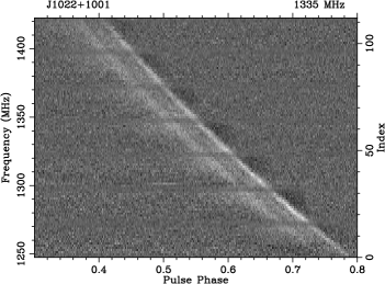
Figure 18: Gray-scale image of the profile against frequency obtained from the Effelsberg at MJD 55974 with 4-hr integration time.

Figure 19: Pulse profiles formed with a bandwidth of 3 MHz at the lower (left) and upper (right) side of the 1285 MHz sub-band, respectively, from the data shown in Fig. 18. The central frequencies are 1277 and 1293 MHz, respectively.

Fig. 20 shows the polarisation profile of data in Fig. 18. It can be seen that the linear and circular components in general retain their original shape, while the total intensity profile is greatly suppressed and lower than the linear component at most of the on-pulse phases including the valley region between the two main peaks. This explains why the WSRT profile shown in Fig. 1 is slightly over-polarised.

Figure 20: Polarisation profile of the data in Fig. 18, averaging over all frequencies.

References

- Antoniadis et al. (2013) Antoniadis J. et al., 2013, Science, 340, 448
- Cairns (2004) Cairns I. H., 2004, ApJ, 610, 948
- Cognard et al. (1996) Cognard I., Shrauner J. A., Taylor J. H., Thorsett S. E., 1996, ApJ, 457, 81
- Cordes & Lazio (2002) Cordes J. M., Lazio T. J. W., 2002, astro-ph/0207156
- Cordes & Shannon (2010) Cordes J. M., Shannon R. M., 2010, astro-ph/1107.3086
- Demorest et al. (2013) Demorest P. B. et al., 2013, ApJ, 762, 94
- Demorest et al. (2010) Demorest P. B., Pennucci T., Ransom S. M., Roberts M. S. E., Hessels J. W. T., 2010, Nature, 467, 1081
- Dyks et al. (2004) Dyks J., Rudak B., Harding A. K., 2004, ApJ, 607, 939
- Edwards & Stappers (2003a) Edwards R. T., Stappers B. W., 2003a, A&A, 407, 273
- Edwards & Stappers (2003b) Edwards R. T., Stappers B. W., 2003b, A&A, 407, 273
- Freire et al. (2012) Freire P. C. C. et al., 2012, MNRAS, 423, 3328
- Hobbs et al. (2006) Hobbs G. B., Edwards R. T., Manchester R. N., 2006, MNRAS, 369, 655
- Hotan et al. (2004) Hotan A. W., Bailes M., Ord S. M., 2004, MNRAS, 355, 941
- Hotan et al. (2004) Hotan A. W., van Straten W., Manchester R. N., 2004, Proc. Astr. Soc. Aust., 21, 302
- Jenet et al. (1998) Jenet F., Anderson S., Kaspi V., Prince T., Unwin S., 1998, ApJ, 498, 365
- Jenet & Anderson (1998) Jenet F. A., Anderson S. B., 1998, PASP, 110, 1467
- Jenet et al. (2001) Jenet F. A., Anderson S. B., Prince T. A., 2001, ApJ, 546, 394
- Joshi et al. (2004) Joshi B. C., Kramer M., Lyne A. G., McLaughlin M. A., Stairs I. H., 2004, in Camilo F., Gaensler B. M., ed, IAU Symposium, p. 319
- Karuppusamy et al. (2008) Karuppusamy R., Stappers B., van Straten W., 2008, PASP, 120, 191
- Knight et al. (2005) Knight H. S., Bailes M., Manchester R. N., Ord S. M., 2005, ApJ, 625, 951
- Kramer (1994) Kramer M., 1994, A&AS, 107, 527
- Kramer et al. (2006) Kramer M. et al., 2006, Science, 314, 97
- Kramer & Stappers (2010) Kramer M., Stappers B., 2010, in ISKAF2010 Science Meeting
- Kramer et al. (1999) Kramer M., Xilouris K. M., Camilo F., Nice D., Lange C., Backer D. C., Doroshenko O., 1999, ApJ, 520, 324
- Liu et al. (2012) Liu K., Keane E. F., Lee K. J., Kramer M., Cordes J. M., Purver M. B., 2012, MNRAS, 420, 361
- Liu et al. (2011) Liu K., Verbiest J. P. W., Kramer M., Stappers B. W., van Straten W., Cordes J. M., 2011, MNRAS, 417, 2916
- Manchester (2013) Manchester R. N., 2013, Class. Quant Grav. in press, astro-ph/1309.7392
- Manchester et al. (2005) Manchester R. N., Hobbs G. B., Teoh A., Hobbs M., 2005, AJ, 129, 1993
- Ord et al. (2004) Ord S. M., van Straten W., Hotan A. W., Bailes M., 2004, MNRAS, 352, 804
- Osłowski et al. (2014) Osłowski S., van Straten W., Bailes M., Jameson A., Hobbs G., 2014, MNRAS, 441, 3148
- Osłowski et al. (2013) Osłowski S., van Straten W., Demorest P., Bailes M., 2013, MNRAS, 430, 416
- Osłowski et al. (2011) Osłowski S., van Straten W., Hobbs G. B., Bailes M., Demorest P., 2011, MNRAS, 418, 1258
- Özel et al. (2010) Özel F., Psaltis D., Ransom S., Demorest P., Alford M., 2010, ApJ, 724, L199
- Pétri (2011) Pétri J., 2011, MNRAS, 412, 1870
- Press et al. (1986) Press W. H., Flannery B. P., Teukolsky S. A., Vetterling W. T., 1986, Numerical Recipes: The Art of Scientific Computing. Cambridge University Press, Cambridge
- Purver (2010) Purver M. B., 2010, Ph.D. thesis, University of Manchester
- Ramachandran & Kramer (2003) Ramachandran R., Kramer M., 2003, A&A, 407, 1085
- Romani & Johnston (2001) Romani R., Johnston S., 2001, ApJ, 557, L93
- Shannon & Cordes (2012) Shannon R. M., Cordes J. M., 2012, ApJ, 761, 64
- Shannon et al. (2013) Shannon R. M. et al., 2013, Science, 342, 334
- Stairs et al. (1999) Stairs I. H., Thorsett S. E., Camilo F., 1999, ApJS, 123, 627
- Taylor (1992) Taylor J. H., 1992, Phil. Trans. Roy. Soc. A, 341, 117
- van Haasteren et al. (2011) van Haasteren R. et al., 2011, MNRAS, 414, 3117
- van Straten (2004) van Straten W., 2004, ApJ, 152, 129
- van Straten (2006) van Straten W., 2006, ApJ, 642, 1004
- van Straten (2013) van Straten W., 2013, ApJS, 204, 13
- van Straten & Bailes (2011) van Straten W., Bailes M., 2011, Proc. Astr. Soc. Aust., 28, 1
- Verbiest et al. (2009) Verbiest J. P. W. et al., 2009, MNRAS, 400, 951
- Weltevrede et al. (2012) Weltevrede P., Wright G., Johnston S., 2012, MNRAS, 424, 843
- Yardley et al. (2011) Yardley D. R. B. et al., 2011, MNRAS, 414, 1777
- You et al. (2007) You X.-P. et al., 2007, MNRAS, 378, 493