Information Geometry Formalism for the Spatially Homogeneous Boltzmann Equation

Abstract.

Information Geometry generalizes to infinite dimension by modeling the tangent space of the relevant manifold of probability densities with exponential Orlicz spaces. We review here several properties of the exponential manifold on a suitable set $\mathcal{E}$ of mutually absolutely continuous densities. We study in particular the fine properties of the Kullback-Liebler divergence in this context. We also show that this setting is well-suited for the study of the spatially homogeneous Boltzmann equation if $\mathcal{E}$ is a set of positive densities with finite relative entropy with respect to the Maxwell density. More precisely, we analyse the Boltzmann operator in the geometric setting from the point of its Maxwell’s weak form as a composition of elementary operations in the exponential manifold, namely tensor product, conditioning, marginalization and we prove in a geometric way the basic facts i.e., the H-theorem. We also illustrate the robustness of our method by discussing, besides the Kullback-Leibler divergence, also the property of Hyvärinen divergence. This requires to generalise our approach to Orlicz-Sobolev spaces to include derivatives.

1. Introduction

Information geometry (IG) has been essentially developed by S.-I. Amari, see the monograph by Amari and Nagaoka [4]. In his work, all previous geometric—essentially metric—descriptions of probabilistic and statistics concepts are extended in the direction of affine differential geometry, including the fundamental treatment of connections. A corresponding concept for abstract manifold, called statistical manifold, has been worked out by S. L. Lauritzen in [3]. Amari’s framework is today considered a case of Hessian geometry as it is described in the monograph by H. Shima [38].

Other versions of IG have been studied to deal with a non-parametric settings such as the Boltzmann equation as it is described in [14] and [41]. A very general set-up for information geometry is the following. Consider a one-dimensional family of positive densities with respect to a measure $\mu$, $\theta\mapsto p_{\theta}$, and a random variable $U$. A classical statistical computation, possibly due to Ronald Fisher, is

$$\frac{d}{d\theta}\int U(x)p(x;\theta)\ \mu(dx)=\int U(x)\left(\frac{d}{d\theta}p(x;\theta)\right)\ \mu(dx)=\\ \int U(x)\left(\frac{d}{d\theta}\log p(x;\theta)\right)\ p(x;\theta)\ \mu(dx)={\operatorname{\mathbb{E}}}_{\theta}\left[\left(U-{\operatorname{\mathbb{E}}}_{\theta}\left[U\right]\right)\frac{d}{d\theta}\log p_{\theta}\right]\ .$$

The previous computation suggests the following geometric construction which is rigorous if the sample space is finite and can be forced to work in general under suitable assumptions. We use the differential geometry language e.g., [17]. If $\Delta$ is the probability simplex on a given sample space $(\Omega,\mathcal{F})$, we define the statistical bundle of $\Delta$ to be

$$T\Delta=\left\{(\pi,u)\middle|\pi\in\Delta,u\in\mathcal{L}^{2}(\pi),{\operatorname{\mathbb{E}}}_{\pi}\left[u\right]=0\right\}.$$

Given a one dimensional curve in $\Delta$, $\theta\mapsto\pi_{\theta}$ we can define its velocity to be the curve

$$\theta\mapsto\left(\pi_{\theta},\frac{D}{d\theta}\pi_{\theta}\right)\in T\Delta\ ,$$

where we define

$$\frac{D}{d\theta}\pi_{\theta}=\frac{d}{d\theta}\log\left(\pi_{\theta}\right)=\dfrac{\frac{d}{d\theta}\pi_{\theta}}{\pi_{\theta}}\ .$$

Each fiber $T_{\pi}\Delta=\mathcal{L}_{0}^{2}(\mu)$ has a scalar product and we have a parallel transport

$$\mathbb{U}_{\pi}^{\nu}\colon T_{\pi}\Delta\ni V\mapsto V-{\operatorname{\mathbb{E}}}_{\nu}\left[V\right]\in T_{\nu}\Delta\ .$$

This structure provides an interesting framework to interpret the Fisher computation cited above. The basic case of a finite state space has been extended by Amari and coworkers to the case of a parametric set of strictly positive probability densities on a generic sample space. Following a suggestion by A. P. Dawid in [18, 16], a particular nonparametric version of that theory was developed in a series of papers [36, 20, 35, 19, 12, 13, 22, 31, 32, 34, 33], where the set $\mathcal{P}_{>}$ of all strictly positive probability densities of a measure space is shown to be a Banach manifold (as it is defined in [8, 1, 24]) modeled on an Orlicz Banach space, see e.g., [28, Chapter II].

In the present paper, Sec. 2 recalls the theory and our notation about the model Orlicz spaces. This material is included for convenience only and this part should be skipped by any reader aware of any of the papers [36, 20, 35, 19, 12, 13, 22, 31, 32, 34, 33] quoted above. The following Sec. 3 is mostly based on the same references and it is intended to introduce that manifold structure and to give a first example of application to the study of Kullback-Liebler divergence. The special features of statistical manifolds that contain the Maxwell density are discussed in Sec. 4. In this case we can define the Boltzmann-Gibbs entropy and study its gradient flow. The setting for the Boltzmann equation is discussed in Sec. 5 where we show that the equation can be derived from probabilistic operations performed on the statistical manifold. Our application to the study of the Kullback-Liebler divergence is generalised in Sec. 6 to the more delicate case of the Hyvarïnen divergence. This requires in particular a generalisation of the manifold structure to include differential operators and leads naturally to the introduction of Orlicz-Sobolev spaces.

We are aware that there are other approaches to non-parametric information geometry that are not based on the notion of the exponential family and that we do not consider here. We mention in particular [29] and [7].

2. Model Spaces

Given a $\sigma$-finite measure space, $(\Omega,\mathcal{F},\mu)$, we denote by $\mathcal{P}_{>}$ the set of all densities that are positive $\mu$-a.s, by $\mathcal{P}_{\geqslant}$ the set of all densities, by $\mathcal{P}_{1}$ the set of measurable functions $f$ with $\int f\ d\mu=1$.

We introduce here the Orlicz spaces we shall mainly investigate in the sequel. We refer to [13] and [28, Chapter II] for more details on the matter. We consider the Young function

$$\Phi\colon\mathbb{R}\ni x\mapsto\Phi(x)=\cosh x-1$$

and, for any $p\in\mathcal{P}_{>}$, the Orlicz space $L^{\Phi}(p)=L^{\cosh-1}\left(p\right)$ is defined as follows: a real random variable $U$ belongs to $L^{\Phi}(p)$ if

$${\operatorname{\mathbb{E}}}_{p}\left[\Phi(\alpha U)\right]<+\infty\qquad\text{ for some }\quad\alpha>0\ .$$

The Orlicz space $L^{\Phi}(p)$ is a Banach space when endowed with the Luxemburg norm defined as

$$\|U\|_{\Phi,p}=\inf\left\{\lambda>0\middle|\,{\operatorname{\mathbb{E}}}_{p}\left[\Phi(U/\lambda)\right]\leqslant 1\right\}\ .$$

The conjugate function of $\Phi=\cosh-1$ is

$$\Phi_{*}(y)=(\cosh-1)_{*}(y)=\int_{0}^{y}\operatorname{arsinh}u\ du=y\operatorname{arsinh}y+1-\sqrt{1+y^{2}},\qquad y\in\mathbb{R}$$

which satisfies the so-called $\Delta_{2}$-condition as

$$\Phi_{*}(\alpha\,y)=\int_{0}^{\left|\alpha y\right|}\left(\left|\alpha y\right|-u\right)\Phi_{*}^{\prime\prime}(u)du=\int_{0}^{\left|\alpha y\right|}\frac{\left|\alpha\right|\left|y\right|-u}{1+u^{2}}\ du\leqslant\max(1,\alpha^{2})\Phi_{*}(y)\ .$$

Since $\Phi_{*}$ is a Young function, for any $p\in\mathcal{P}_{>}$, one can define as above the associated Orlicz space $L^{\Phi_{*}}(p)=L^{(\cosh-1)_{*}}\left(p\right)$ and its corresponding Luxemburg norm $\|\cdot\|_{\Phi_{*},p}.$ Because the functions $\Phi$ and $\Phi_{*}$ form a Young pair, for each $U\in L^{\cosh-1}(p)$ and $V\in L^{(\cosh-1)_{*}}(p)$ we can deduce from Young’s inequality

$$xy\leqslant\Phi(x)+\Phi_{*}(y)\qquad\forall x,y\in\mathbb{R}^{2},$$

that the following Holder’s inequality holds:

$$\left|{\operatorname{\mathbb{E}}}_{p}\left[UV\right]\right|\leqslant 2\left\|U\right\|_{\cosh-1,p}\,\left\|V\right\|_{(\cosh-1)_{*},p}<\infty\ .$$

Moreover, it is a classical result that the space $L^{(\cosh-1)_{*}}(p)$ is separable and its dual space is $L^{\cosh-1}(p)$, the duality pairing being

$$(V,U)\in L^{(\cosh-1)_{*}}(p)\times L^{\cosh-1}(p)\longmapsto\left\langle U,V\right\rangle_{p}:={\operatorname{\mathbb{E}}}_{p}\left[UV\right]\ .$$

We recall the following continuous embedding result that we shall use repeatedly in the paper:

Theorem 1.

Given $p\in\mathcal{P}_{>}$, for any $1<r<\infty$, the following embeddings

$$L^{\infty}(p)\hookrightarrow L^{\cosh-1}\left(p\right)\hookrightarrow L^{r}(p)\hookrightarrow L^{(\cosh-1)_{*}}\left(p\right)\hookrightarrow L^{1}(p)$$

are continuous.

From this result, we deduce easily the following useful Lemma

Lemma 2.

Given $p\in\mathcal{P}_{>}$ and $k\geqslant 1.$ For any $u_{1},\ldots,u_{k}\in L^{\cosh-1}\left(p\right)$ one has

$$\prod_{i=1}^{k}u_{i}\in\bigcap_{1<r<\infty}L^{r}(p)\ .$$

Proof.

According to Theorem 1, $u_{i}\in L^{r}(p)$ for any $1<r<\infty$ and any $i=1,\ldots,k$. The proof follows then simply from the repeated use of Holder inequality. ∎

From now on we also define, for any $p\in\mathcal{P}_{>}$

$$B_{p}=L^{\Phi}_{0}(p):=\left\{u\in L^{\cosh-1}\left(p\right)\middle|{\operatorname{\mathbb{E}}}_{p}\left[u\right]=0\right\}\ .$$

In the same way, we set ${}^{*}B_{p}=L^{\Phi_{*}}_{0}(p):=\left\{u\in L^{(\cosh-1)_{*}}\left(p\right)\middle|{\operatorname{\mathbb{E}}}_{p}\left[u\right]=0\right\}.$

2.1. Cumulant Generating Functional

Let $p\in\mathcal{\mathcal{P}_{>}}$ be given. With the above notations one can define:

Definition 3.

The cumulant generating functional is the mapping

$$K_{p}\colon u\in B_{p}\longmapsto\log{\operatorname{\mathbb{E}}}_{p}\left[\mathrm{e}^{u}\right]\in[0,+\infty]\ .$$

The following result [12, 13] shows the properties of the exponential function as a superposition mapping [6].

Proposition 4.

Let $a\geqslant 1$ and $p\in\mathcal{P}_{>}$ be given.

1. For any $n=0,1,\dots$ and $u\in L^{\Phi}(p)$:

   $$\lambda_{a,n}(u)\colon\left(w_{1},\dots,w_{n}\right)\mapsto\dfrac{w_{1}}{a}\cdots\dfrac{w_{n}}{a}\ \mathrm{e}^{\frac{u}{a}}$$

   is a continuous, symmetric, $n$-multi-linear map from $\left(L^{\Phi}(p)\right)^{n}$ to $L^{a}\left(p\right)$.

2. $v\mapsto\sum_{n=0}^{\infty}\frac{1}{n!}\left(\dfrac{v}{a}\right)^{n}$ is a power series from $L^{\Phi}(p)$ to $L^{a}(p)$, with radius of convergence larger than $1$.

3. The superposition mapping, $v\mapsto\mathrm{e}^{v/a}$, is an analytic function from the open unit ball of $L^{\Phi}(p)$ to $L^{a}(p)$.

The cumulant generating functional enjoys the following properties (see [36, 12, 13]):

Proposition 5.

1. $K_{p}(0)=0$; otherwise, for each $u\neq 0$, $K_{p}(u)>0$.

2. $K_{p}$ is convex and lower semi-continuous, and its proper domain

   $$\mathrm{dom}(K_{p})=\left\{u\in B_{p}\middle|K_{p}(u)<\infty\right\}$$

   is a convex set that contains the open unit ball of $B_{p}$.

3. $K_{p}$ is infinitely Gâteaux-differentiable in the interior of its proper domain.

4. $K_{p}$ is bounded, infinitely Fréchet-differentiable and analytic on the open unit ball of $B_{p}$.

Remark 1.

One sees from the above property 2 that the interior of the proper domain of $K_{p}$ is a non-empty open convex set. From now on we shall adopt the notation

$$\mathcal{S}_{p}=\mathrm{Int}\left(\mathrm{dom}(K_{p})\right)\ .$$

Other properties of the functional $K_{p}$ are described below, as they relate directly to the exponential manifold.

3. Exponential manifold

The set of positive densities, $\mathcal{P}_{>}$, locally around a given $p\in\mathcal{P}_{>}$, is modeled by the subspace of centered random variables in the Orlicz space, $L^{\cosh-1}(p)$. Hence, it is crucial to discuss the isomorphism of the model spaces for different $p$’s in order to show the existence of an atlas defining a Banach manifold.

Definition 6 (Statistical exponential manifold [13, Def. 20]).

For $p\in\mathcal{P}_{>}$, the statistical exponential manifold at $p$ is

$${\mathcal{E}}\left(p\right)=\left\{\mathrm{e}^{u-K_{p}(u)}p\middle|u\in\mathcal{S}_{p}\right\}\ .$$

We also need the following definition of connection

Definition 7 (Connected densities).

Densities $p,q\in\mathcal{P}_{>}$ are connected by an open exponential arc if there exists an open exponential family containing both, i.e., if for a neighborhood $I$ of $[0,1]$

$$\int_{\Omega}p^{1-t}q^{t}\ d\mu={\operatorname{\mathbb{E}}}_{p}\left[\left(\frac{q}{p}\right)^{t}\right]={\operatorname{\mathbb{E}}}_{q}\left[\left(\frac{p}{q}\right)^{1-t}\right]<+\infty,\quad t\in I$$

In such a case, one simply writes $p\smile q.$

Theorem 8 (Portmanteau theorem [13, Th 19 and 21],[37, Theorem 4.7]).

Let $p,q\in\mathcal{P}_{>}.$ The following statements are equivalent:

1. $p\smile q$ (i.e. $p$ and $q$ are connected by an open exponential arc);

2. $q\in{\mathcal{E}}\left(p\right)$;

3. ${\mathcal{E}}\left(p\right)={\mathcal{E}}\left(q\right)$;

4. $\log\frac{q}{p}\in L^{\Phi}(p)\cap L^{\Phi}(q)$;

5. $L^{\Phi}(p)=L^{\Phi}(q)$ (i.e. they both coincide as vector spaces and their norms are equivalent);

6. There exists $\varepsilon>0$ such that

   $$\frac{q}{p}\in L^{1+\varepsilon}(p)\quad\text{ and }\quad\frac{p}{q}\in L^{1+\varepsilon}(q)\$$

We can now define the charts and atlas of the exponential manifold as follows:

Definition 9 (Exponential manifold [36, 35, 12, 13]).

For each $p\in\mathcal{P}_{>}$, define the charts at $p$ as:

$$s_{p}\>\colon\>q\in{\mathcal{E}}\left(p\right)\longmapsto\log\left(\frac{q}{p}\right)-{\operatorname{\mathbb{E}}}_{p}\left[\log\left(\frac{q}{p}\right)\right]\in\mathcal{S}_{p}\subset B_{p},$$

with inverse

$$s_{p}^{-1}=e_{p}\>\colon\>u\in\mathcal{S}_{p}\mapsto\mathrm{e}^{u-K_{p}(u)}p\in{\mathcal{E}}\left(p\right)\subset\mathcal{P}_{>}$$

The atlas, $\left\{s_{p}\colon\mathcal{S}_{p}\middle|p\in\mathcal{P}_{>}\right\}$ is affine and defines the exponential (statistical) manifold $\mathcal{P}_{>}$.

We collect here various results from [36, 35, 12, 13] about additional properties of $K_{p}$.

Proposition 10.

Let $q=\mathrm{e}^{u-K_{p}(u)}p\in{\mathcal{E}}\left(p\right)$ with $u\in\mathcal{S}_{p}$.

1. The first three derivatives of $K_{p}$ on $\mathcal{S}_{p}$ are:

   $$dK_{p}(u)[v] ={\operatorname{\mathbb{E}}}_{q}\left[v\right]\ ,$$

   $$d^{2}K_{p}(u)[v_{1},v_{2}] =\operatorname{Cov}_{q}\left(v_{1},v_{2}\right)\ ,$$

   $$d^{3}K_{p}(u)[v_{1},v_{2},v_{3}] =\operatorname{Cov}_{q}(v_{1},v_{2},v_{3})\ .$$

2. The random variable, $\dfrac{q}{p}-1$, belongs to $\prescript{*}{}{B}_{p}$ and:

   $$d{K_{p}(u)}[v]={\operatorname{\mathbb{E}}}_{p}\left[\left(\frac{q}{p}-1\right)v\right]\ .$$

   In other words, the gradient of $K_{p}$ at $u$ is identified with an element of the predual space of $B_{p}$, viz. $\prescript{*}{}{B}_{p}$, denoted by $\nabla K_{p}(u)=e^{u-K_{p}(u)}-1=\dfrac{q}{p}-1$.

3. The weak derivative of the map, $\mathcal{S}_{p}\ni u\mapsto\nabla K_{p}(u)\in\prescript{*}{}{B}_{p}$, at $u$ applied to $w\in B_{p}$ is given by:

   $$d(\nabla K_{p}(u)){[w]}=\frac{q}{p}\left(w-{\operatorname{\mathbb{E}}}_{q}\left[w\right]\right)$$

   and it is one-to-one at each point.

4. $q/p\in L^{(\cosh-1)_{*}}(p)$.

5. $B_{q}$ is defined by an orthogonality property:

   $$B_{q}=L_{0}^{\cosh-1}(q)=\left\{u\in L^{\cosh-1}(p)\middle|{\operatorname{\mathbb{E}}}_{p}\left[u\frac{q}{p}\right]=0\right\}\ .$$

On the basis of the above result, it appears natural to define the following parallel transports:

Definition 11.

1. The exponential transport $\prescript{\text{e}}{}{\mathbb{U}}_{p}^{q}\colon B_{p}\to B_{q}$ is computed as

   $$\prescript{\text{e}}{}{\mathbb{U}}_{p}^{q}u=u-{\operatorname{\mathbb{E}}}_{q}\left[u\right]\qquad u\in B_{p}\ .$$

2. The mixture transport $\prescript{\text{m}}{}{\mathbb{U}}_{q}^{p}\colon\prescript{*}{}{B}_{q}\to\prescript{*}{}{B}_{p}$ is computed as

   $$\prescript{\text{m}}{}{\mathbb{U}}_{q}^{p}v=\frac{p}{q}v\qquad v\in\prescript{*}{}{B}_{q}\ .$$

One has the following properties

Proposition 12.

Let $p,q\in\mathcal{P}_{>}$ be given. Then

1. $\prescript{\text{e}}{}{\mathbb{U}}_{p}^{q}$ is an isomorphism of $B_{p}$ onto $B_{q}$.

2. $\prescript{\text{m}}{}{\mathbb{U}}_{q}^{p}$ is an isomorphism of $\prescript{*}{}{B}_{q}$ onto $\prescript{*}{}{B}_{p}$.

3. The mixture transport $\prescript{\text{m}}{}{\mathbb{U}}_{q}^{p}$ and the exponential transport $\prescript{\text{e}}{}{\mathbb{U}}_{p}^{q}$ are dual of each other: if $u\in B_{q}$ and $v\in\prescript{*}{}{B}_{p}$ then

   $$\left\langle u,\prescript{\text{m}}{}{\mathbb{U}}_{p}^{q}v\right\rangle_{q}=\left\langle\prescript{\text{e}}{}{\mathbb{U}}_{q}^{p}u,v\right\rangle_{p}\ .$$

4. $\prescript{\text{m}}{}{\mathbb{U}}_{p}^{q}$ and $\prescript{\text{e}}{}{\mathbb{U}}_{p}^{q}$ together transport the duality pairing: if $u\in B_{p}$ and $v\in\prescript{*}{}{B}_{p}$, then

   $$\left\langle u,v\right\rangle_{p}=\left\langle\prescript{\text{e}}{}{\mathbb{U}}_{p}^{q}u,\prescript{\text{m}}{}{\mathbb{U}}_{p}^{q}v\right\rangle_{q}.$$

We reproduce here a scheme of how the affine manifold works. The domains of the charts centered at $p$ and $q$ respectively are either disjoint or equal if $p\smile q$:

Our discussion of the tangent bundle of the exponential manifold is based on the concept of the velocity of a curve as in [1, §3.3] and it is mainly intended to underline its statistical interpretation, which is obtained by identifying curves with one-parameter statistical models. For a statistical model $p(t)$, $t\in I$, the random variable, $\dot{p}(t)/p(t)$ (which corresponds to the Fisher score), has zero expectation with respect to $p(t)$, and its meaning in the exponential manifold is velocity; see [11] on exponential families. More precisely, let $p(\cdot)\colon I\to{\mathcal{E}}\left(p\right)$, $I$ the open real interval containing zero. In the chart centered at $p$, the curve is $u(\cdot)\colon I\to B_{p}$, where $p(t)=\mathrm{e}^{u(t)-K_{p}(u(t))}p$.

Definition 13 (Velocity field of a curve and tangent bundle).

1. Assume $t\mapsto u(t)=s_{p}(p(t))$ is differentiable with derivative $\dot{u}(t)$. Define:

   (1) $$\frac{D}{dt}p(t)=\prescript{\text{e}}{}{\mathbb{U}}_{p}^{p(t)}\dot{u}(t)=\dot{u}(t)-{\operatorname{\mathbb{E}}}_{p(t)}\left[\dot{u}(t)\right]=\frac{d}{dt}{(u(t)-K_{p}(u(t))}=\frac{d}{dt}{\log\left(\frac{p(t)}{p}\right)}=\frac{\frac{d}{dt}p(t)}{p(t)}\ .$$

   Note that $Dp$ does not depend on the chart $s_{p}$ and that the derivative of $t\mapsto p(t)$ in the last term of the equation is computed in $L^{\Phi_{*}}(p)$. The curve $t\mapsto(p(t),Dp(t))$ is the velocity field of the curve.

2. On the set $\left\{(p,v)\middle|p\in\mathcal{P}_{>},v\in B_{p}\right\}$, the charts:

   (2) $$s_{p}\colon\left\{(q,w)\middle|q\in{\mathcal{E}}\left(p\right),w\in B_{q}\right\}\ni(q,w)\mapsto(s_{p}(q),\prescript{\text{e}}{}{\mathbb{U}}_{q}^{p}w)\in\mathcal{S}_{p}\times B_{p}\subset B_{p}\times B_{p}$$

   define the tangent bundle, $T\mathcal{P}_{>}$.

Remark 2.

Let $E\colon{\mathcal{E}}\left(p\right)\to\mathbb{R}$ be a $C^{1}$ function. Then, $E_{p}=E\circ e_{p}\colon\mathcal{S}_{p}\to\mathbb{R}$ is differentiable and:

$$\frac{d}{dt}E(p(t))=\frac{d}{dt}E_{p}(u(t))=dE_{p}(u(t))\dot{u}(t)=dE_{p}(u(t))\prescript{\text{e}}{}{\mathbb{U}}_{p(t)}^{p}Dp(t)$$

3.1. Pretangent Bundle

Let $M$ be a density and ${\mathcal{E}}\left(M\right)$ its associated exponential manifold. Here $M$ is generic, later it will be the Maxwell distribution. All densities are assumed to be in ${\mathcal{E}}\left(M\right)$.

Definition 14 (Pretangent bundle $\prescript{*}{}{T}{\mathcal{E}}\left(p\right)$).

The set

$$\prescript{*}{}{T}{\mathcal{E}}\left(M\right)=\left\{(q,V)\middle|q\in{\mathcal{E}}\left(M\right),V\in\prescript{*}{}{B}_{q}\right\}$$

together with the charts:

$$\prescript{*}{}{s}_{p}\colon\prescript{*}{}{T}{\mathcal{E}}\left(M\right)\ni(q,V)\mapsto\left(s_{p}(q),\prescript{\text{m}}{}{\mathbb{U}}_{q}^{p}V\right)$$

is the pretangent bundle, $\prescript{*}{}{T}{\mathcal{E}}\left(M\right)$.

Let $F$ be a vector field of the pretangent bundle, $F\colon{\mathcal{E}}\left(M\right)\to\prescript{*}{}{T}{\mathcal{E}}\left(M\right)$. In the chart centered at $p$, the vector field is expressed by

$$F_{p}(u)=\prescript{\text{m}}{}{\mathbb{U}}_{e_{p}(u)}^{p}{F\circ e_{p}(u)}=\frac{e_{p}(u)}{p}F\circ e_{p}(u)\in\prescript{*}{}{B}_{p},\quad u\in\mathcal{S}_{M}$$

If $F_{p}$ is of class $C^{1}$ with derivative $dF_{p}(u)\in L(B_{p},\prescript{*}{}{B}_{p})$, for each differentiable curve $t\mapsto p(t)=\mathrm{e}^{U(t)-K_{p}(U(t))}\cdot p$ we have $Dp(t)=\frac{d}{dt}\log p(t)=\dot{U}(t)-{\operatorname{\mathbb{E}}}_{p(t)}\left[\dot{U}(t)\right]$ and also

$$\frac{d}{dt}F_{p}(U(t))=dF_{p}(U(t))[\dot{u}(t)]=dF_{p}(u(t))[\prescript{\text{e}}{}{\mathbb{U}}_{p(t)}^{p}{Dp(t)}]\in\prescript{*}{}{B}_{p}$$

Definition 15 (Covariant derivative in $\prescript{*}{}{T}{\mathcal{E}}\left(M\right)$).

Let $F$ be a vector field of class $C^{1}$ of the pretangent bundle $\prescript{*}{}{T}{\mathcal{E}}\left(M\right)$, and let $G$ be a continuous vector field in the tangent bundle $T{\mathcal{E}}\left(M\right)$. The covariant derivative is the vector field $D_{G}F$ of $\prescript{*}{}{T}{\mathcal{E}}\left(M\right)$ defined at each $q\in{\mathcal{E}}\left(M\right)$ by

$$(D_{G}F)(q)=\left.dF_{q}(u)\right|_{u=0}[w],\quad w=G(q)$$

In the definition above the covariant derivative is computed in the mobile frame because its value at $q$ is computed using the expression in the chart centered at $q$. In a fixed frame centered at $p$ we write $s_{p}(q)=w$ so that $e_{q}(u)=e_{p}(u-{\operatorname{\mathbb{E}}}_{p}\left[u\right]+w)$, and compare the two expressions of $F$ as follows.

$$F_{q}(u)=\prescript{\text{m}}{}{\mathbb{U}}_{e_{q}(u)}^{q}F\circ e_{q}(u)=\\ \prescript{\text{m}}{}{\mathbb{U}}_{e_{q}(u)}^{q}\prescript{\text{m}}{}{\mathbb{U}}_{p}^{e_{p}(u-{\operatorname{\mathbb{E}}}_{p}\left[u\right]+w)}\prescript{\text{m}}{}{\mathbb{U}}_{e_{p}(u-{\operatorname{\mathbb{E}}}_{p}\left[u\right]+w)}^{p}F\circ e_{p}(u-{\operatorname{\mathbb{E}}}_{p}\left[u\right]+w)=\\ \prescript{\text{m}}{}{\mathbb{U}}_{p}^{q}\prescript{\text{m}}{}{\mathbb{U}}_{e_{p}(u-{\operatorname{\mathbb{E}}}_{p}\left[u\right]+w)}^{p}F\circ e_{p}(u-{\operatorname{\mathbb{E}}}_{p}\left[u\right]+w)=\prescript{\text{m}}{}{\mathbb{U}}_{p}^{q}F_{p}(u-{\operatorname{\mathbb{E}}}_{p}\left[u\right]+w).$$

Derivation in the direction $v\in B_{q}$ gives

$$dF_{q}(u)[v]=\prescript{\text{m}}{}{\mathbb{U}}_{p}^{q}dF_{p}(u-{\operatorname{\mathbb{E}}}_{p}\left[u\right]+w)[v-{\operatorname{\mathbb{E}}}_{p}\left[v\right]],$$

hence $dF_{q}(u)=\prescript{\text{m}}{}{\mathbb{U}}_{p}^{q}dF_{p}(\prescript{\text{e}}{}{\mathbb{U}}_{q}^{p}u+w)\prescript{\text{e}}{}{\mathbb{U}}_{q}^{p}$ and at $u=0$, we have $dF_{q}(0)=\prescript{\text{m}}{}{\mathbb{U}}_{p}^{q}dF_{p}(w)\prescript{\text{e}}{}{\mathbb{U}}_{q}^{p}$. It follows that the covariant derivative in the fixed frame at $p$ is

$$(D_{G}F)(q)=\prescript{\text{m}}{}{\mathbb{U}}_{p}^{q}dF_{p}(s_{p}(q))\prescript{\text{e}}{}{\mathbb{U}}_{q}^{p}G(q).$$

The tangent and pretangent bundle can be coupled to produce the vector bundle of order 2 defined by

$$(\prescript{*}{}{T}\times T){\mathcal{E}}\left(M\right)=\left\{(p,v,w)\middle|p\in{\mathcal{E}}\left(M\right),v\in B_{p},w\in\prescript{*}{}{B}_{p}\right\}$$

with charts

$$(q,v,w)\mapsto(s_{p}(q),\prescript{\text{e}}{}{\mathbb{U}}_{q}^{p}v,\prescript{\text{m}}{}{\mathbb{U}}_{q}^{p}w)$$

and the duality coupling:

$$(q,v,w)\mapsto\left\langle\prescript{\text{e}}{}{\mathbb{U}}_{q}^{p}v,\prescript{\text{m}}{}{\mathbb{U}}_{q}^{p}w\right\rangle_{q}$$

Proposition 16 (Covariant derivative of the duality coupling).

Let $F$ be a vector field of $\prescript{*}{}{T}{\mathcal{E}}\left(M\right)$, and let $G,X$ be vector fields of $T{\mathcal{E}}\left(M\right)$, $F,G$ of class $C^{1}$ and $X$ continuous.

$$D_{X}\left\langle F,G\right\rangle=\left\langle D_{X}F,G\right\rangle+\left\langle F,D_{X}G\right\rangle$$

Proof.

Consider the real function $\mathcal{E}\ni q\mapsto\left\langle F,G\right\rangle(q)={\operatorname{\mathbb{E}}}_{q}\left[F(q)G(q)\right]$ in the chart centered at any $p\in{\mathcal{E}}\left(M\right)$:

$$\mathcal{S}_{p}\ni u\mapsto{\operatorname{\mathbb{E}}}_{e_{p}(u)}\left[F(e_{p}(u))G(e_{p}(u))\right]=\\ {\operatorname{\mathbb{E}}}_{p}\left[\prescript{\text{m}}{}{\mathbb{U}}_{e_{p}(u)}^{p}{F\circ e_{p}(u)}\prescript{\text{e}}{}{\mathbb{U}}_{e_{p}(u)}^{p}{G\circ e_{p}(u)}\right]={\operatorname{\mathbb{E}}}_{p}\left[F_{p}(u)G_{p}(u)\right],$$

and compute its derivative at 0 in the direction $X(p)$. ∎

We refer to [34, 33] for further details on the geometric structure, namely the Hilbert bundle, the tangent mapping of an homeomorphism, the Riemannian Hessian. We now turn to a basic example.

3.2. Kullback-Leibler Divergence

The Kullback-Leibler divergence [23] on the exponential manifold $\mathcal{E}$ is the mapping

$$\mathbf{D}\>\colon\>(q_{1},q_{2})\in\mathcal{E}\times\mathcal{E}\longmapsto\mathbf{D}\left(q_{1}\,\|q_{2}\right)={\operatorname{\mathbb{E}}}_{q_{1}}\left[\log\left(\frac{q_{1}}{q_{2}}\right)\right].$$

Notice that, if $q_{2}=\mathrm{e}^{u-K_{q_{1}}(u)}\cdot q_{1}\in{\mathcal{E}}\left(q_{1}\right)$, $u\in\mathcal{S}_{q_{1}}$, then $K_{q_{1}}(u)={\operatorname{\mathbb{E}}}_{q_{1}}\left[\log\left(q_{1}/q_{2}\right)\right]$ is the expression in the chart centered at $q_{1}$ of the marginal Kullback-Leibler divergence $q_{2}\mapsto\mathbf{D}\left(q_{1}\,\|q_{2}\right)$. Therefore, the Kullback-Leibler divergence is non-negative valued and zero if and only if $q_{2}=q_{1}$ because of Theorem 8, item (4). Its expression in the chart centered at a generic $p\in\mathcal{E}$ is

$$D_{p}\>\colon\>(u_{1},u_{2})\in\mathcal{S}_{p}\times\mathcal{S}_{p}\longmapsto K_{p}(u_{2})-K_{p}(u_{1})-dK_{p}(u_{1})[u_{2}-u_{1}]\ ,$$

which is the Bregman divergence [9] of the convex function $K_{p}\colon\mathcal{S}_{p}\to\mathbb{R}$.

It follows from Proposition 5.(4) that it is $C^{\infty}$ jointly in both variables and, moreover, analytic with

$$D_{p}(u_{1},u_{2})=\sum_{n\geqslant 2}\frac{1}{n!}d^{n}K_{p}(u_{1})[(u_{1}-u_{2})^{\otimes n}],\quad\left\|u_{1}-u_{2}\right\|_{\Phi,p}<1.$$

This regularity result is to be compared with what is available when the restriction, $q_{1}\smile q_{2}$, is removed, i.e., the semi-continuity [5, §9.4].

The partial derivative of $D_{p}$ in the first variable, that is the derivative of $u_{1}\mapsto D_{p}(u_{1},u_{2})$, in the direction $v\in B_{p}$ is

$$d(u_{1}\mapsto D_{p}(u_{1},u_{2}))[v]=-d^{2}K_{p}(u_{1})[u_{2}-u_{1},v]=-\operatorname{Cov}_{q_{1}}\left(\log\frac{q_{2}}{q_{1}},v\right),$$

with $\quad q_{i}=\operatorname{e}_{p}(u_{i})$, $i=1,2$. If $v=\prescript{\text{e}}{}{\mathbb{U}}_{q_{1}}^{p}w$, we have $-\operatorname{Cov}_{q_{1}}\left(\log\frac{q_{2}}{q_{1}},v\right)=\operatorname{Cov}_{q_{1}}\left(\log\frac{q_{1}}{q_{2}},w\right)$, so that we can compute both the covariant derivative of the partial functional $q\mapsto\mathbf{D}\left(q\,\|q_{2}\right)$ and its gradient as

$$D_{w}(q\mapsto\mathbf{D}\left(q\,\|q_{2}\right)) =\operatorname{Cov}_{q}\left(\log\frac{q}{q_{2}},w\right)={\operatorname{\mathbb{E}}}_{q}\left[\left(\log\frac{q}{q_{2}}-\mathbf{D}\left(q\,\|q_{2}\right)\right)w\right],$$

$$\nabla(q\mapsto\mathbf{D}\left(q\,\|q_{2}\right)) =\log\frac{q}{q_{2}}-\mathbf{D}\left(q\,\|q_{2}\right).$$

The negative gradient flow is

$$\frac{d}{dt}\log\frac{q(t)}{q_{2}}=-\log\frac{q(t)}{q_{2}}+\mathbf{D}\left(q(t)\,\|q_{2}\right).$$

As $\frac{d}{dt}\left(\mathrm{e}^{t}\log\frac{q(t)}{q_{2}}\right)=\mathrm{e}^{t}\mathbf{D}\left(q(t)\,\|q_{2}\right)$, for each $t$ the random variable

$$\mathrm{e}^{t}\log\frac{q(t)}{q_{2}}-\log\frac{q(0)}{q_{2}}=\mathrm{e}^{t}\log\left(\frac{q(t)}{q_{2}}\left(\frac{q_{2}}{q(0)}\right)^{\mathrm{e}^{-t}}\right)=\mathrm{e}^{t}\log\left(q(t)\frac{q_{2}^{\mathrm{e}^{-t}-1}}{q(0)^{\mathrm{e}^{-t}}}\right)$$

is constant, so that $q(t)\propto q(0)^{\mathrm{e}^{-t}}q_{2}^{1-\mathrm{e}^{-t}}$. It is the exponential arc of $q(0)\smile q_{2}$ in an exponential time scale.

The partial derivative of $D_{p}$ in the second variable, that is the derivative of $u_{2}\mapsto D_{p}(u_{1},u_{2})$, in the direction $v\in B_{p}$ is

$$d(u_{2}\mapsto D_{p}(u_{1},u_{2}))v=dK_{p}(u_{2})[v]-dK_{p}(u_{1})[v]={\operatorname{\mathbb{E}}}_{q_{2}}\left[v\right]-{\operatorname{\mathbb{E}}}_{q_{1}}\left[v\right]\ ,$$

with $\quad q_{i}=\operatorname{e}_{p}(u_{i})$, $i=1,2$. If $v=\prescript{\text{e}}{}{\mathbb{U}}_{q_{2}}^{p}w$, we have ${\operatorname{\mathbb{E}}}_{q_{2}}\left[v\right]-{\operatorname{\mathbb{E}}}_{q_{1}}\left[v\right]={\operatorname{\mathbb{E}}}_{q_{2}}\left[w\right]-{\operatorname{\mathbb{E}}}_{q_{1}}\left[w\right]$, so that we can compute both the covariant derivative of the partial functional $q\mapsto\mathbf{D}\left(q_{1}\,\|q\right)$ and its gradient as

$$D_{w}(q\mapsto\mathbf{D}\left(q_{1}\,\|q\right)) ={\operatorname{\mathbb{E}}}_{q}\left[w\right]-{\operatorname{\mathbb{E}}}_{q_{1}}\left[w\right]={\operatorname{\mathbb{E}}}_{q}\left[\left(1-\frac{q_{1}}{q}\right)w\right],$$

$$\nabla(q\mapsto\mathbf{D}\left(q_{1}\,\|q\right)) =1-\frac{q_{1}}{q}\ .$$

The negative gradient flow is

$$\frac{\dot{q}(t)}{q(t)}=-\left(1-\frac{q_{1}}{q(t)}\right)=\frac{q_{1}-q(t)}{q(t)}\ ,$$

whose solution starting at $q_{0}$ is $q(t)=q_{1}+(q_{0}-q_{1})\mathrm{e}^{-t}$. It is a mixture model in an exponential time scale.

4. Gaussian space

In this Section the sample space is $\mathbb{R}^{n}$, $M$ denotes the standard $n$-dimensional Gaussian density (we denoted it $M$ because of James Clerk Maxwell (1831 – 1879))

(3) $$M(x)=\dfrac{1}{(2\pi)^{n/2}}\exp\left(-\dfrac{|x|^{2}}{2}\right),\qquad x\in\mathbb{R}^{n}$$

and ${\mathcal{E}}$ is the exponential manifold containing $M$. We recall that the Orlicz space $L^{\cosh-1}\left(M\right)$ is defined with the Young function $\Phi:=x\mapsto\cosh x-1$. The following propositions depend on the specific properties of the Gaussian density $M$. They do not hold in general.

Proposition 17.

1. The Orlicz space $L^{\cosh-1}\left(M\right)$ contains all polynomials with degree up to 2.

2. The Orlicz space $L^{(\cosh-1)_{*}}\left(M\right)$ contains all polynomials.

Proof.

1. If $f$ is a polynomial of degree $d\leqslant 2$ then

$$\int_{\mathbb{R}^{n}}\mathrm{e}^{\alpha f(x)}M(x)\ dx=\dfrac{1}{(2\pi)^{n/2}}\int_{\mathbb{R}^{n}}\mathrm{e}^{\alpha f(x)-\frac{1}{2}\left|x\right|^{2}}\ dx$$

and the latter is finite for all $\alpha$ such that $\alpha\operatorname{Hess}f-I$ is negative definite.

2. The result comes from the fact that all polynomials belong to $L^{2}(M)$ and one has $L^{2}(M)\subset L^{(\cosh-1)_{*}}\left(M\right)$.∎

4.1. Boltzmann-Gibbs Entropy

While the Kullback-Leibler divergence $\mathbf{D}\left(q_{1}\,\|q_{2}\right)$ of Sec. 3.2 is defined and finite if the densities $q_{1}$ and $q_{2}$ belong to the same exponential manifold, the Boltzmann-Gibbs entropy (BG-entropy in the sequel)

$$H(q)=-{\operatorname{\mathbb{E}}}_{q}\left[\log\left(q\right)\right]$$

could be either non defined or infinite, precisely $-\infty$, everywhere on some exponential manifolds, or finite everywhere on other exponential manifolds.

Proposition 18.

Assume $p\smile q$, Then:

1. For each $a\geqslant 1$, $\log p\in L^{a}(p)$ if, and only if, $\log q\in L^{a}(q)$.

2. $\log p\in L^{\cosh-1}\left(p\right)$ if, and only if, $\log q\in L^{\cosh-1}\left(q\right)$.

Proof.

If $p,q$ belong to the same exponential manifold, we can write $q=\mathrm{e}^{u-K_{p}(u)}\cdot p$ and, from Theorem 8.(4), we obtain $\log q-\log p=u-K_{p}(u)\in L^{\cosh-1}\left(p\right)=L^{\cosh-1}\left(q\right)$, so that $\log q\in L^{a}(q)$ if, and only if, $\log p\in L^{a}(p)$, $a\geqslant 1$, and $\log q\in L^{\cosh-1}\left(q\right)$ if, and only if, $\log p\in L^{\cosh-1}\left(p\right)$. ∎

In order to obtain a smooth function, we study the BG-entropy $H(q)$ on all manifolds $\mathcal{E}$, such that for at least one, and, hence for all, $p\in\mathcal{E}$, it holds $\log\left(p\right)\in L^{\cosh-1}\left(p\right)$. In such an exponential manifold we can write

$$\mathbf{D}\left(q\,\|p\right)=-H(q)-{\operatorname{\mathbb{E}}}_{q}\left[\log p\right]\ ,$$

so that $H(q)\leqslant-{\operatorname{\mathbb{E}}}_{q}\left[\log p\right]$.

For example, it is the case when the reference measure is finite and $p$ is constant. Another notable example is the Gaussian case, where the sample space is $\mathbb{R}^{n}$ endowed with the Lebesgue measure and $p(x)\propto\exp{-\frac{|x|^{2}}{2}}$. In such case $\int\cosh(\alpha|x|^{2})\exp\left(-|x|^{2}/2\right)\ dx<+\infty$ if $0<\alpha<1/2$.

We investigate here the main properties of the BG-entropy in this context. First, one has

Proposition 19.

The BG-entropy is a smooth real function on the exponential manifold $\mathcal{E}$. Namely, if $p\in\mathcal{E}$ then

$$H_{p}\>:\>u\in\mathcal{S}_{p}\mapsto H\circ e_{p}(u)$$

is a $C^{\infty}$ real function. Moreover, its derivative in the direction $v$ equals

$$dH_{p}(u)[v]=-\operatorname{Cov}_{q}\left(u+\log p,v\right)\ ,$$

where $q=e_{p}(u)$.

Proof.

As

$$-\log q=-u+K_{p}(u)-\log p=-(u+\log p+H(p))+K_{p}(u)+H(p)\in L^{\cosh-1}\left(p\right),$$

with $-(u+\log p+H(p))\in B_{p}$, the representation of the BG-entropy in the chart centered at $p$ is

$$H_{p}(u) =H\circ e_{p}(u)$$

$$=-{\operatorname{\mathbb{E}}}_{e_{p}(u)}\left[u+\log p+H(p)\right]+K_{p}(u)+H(p)$$

$$=-dK_{p}(u)\left[u+\log p+H(p))\right]+K_{p}(u)+H(p)$$

$$=(K_{p}(u)-d_{u}K_{p}(u))-dK_{p}(u)[\log p+H(p)]+H(p),$$

hence, $u\mapsto H_{p}(u)$ is a $C^{\infty}$ real function. Notice that $K_{p}(u)-d_{u}K_{p}(u)\leqslant 0$, hence $H(q)\leqslant{\operatorname{\mathbb{E}}}_{q}\left[\log p\right]$, as we already know. The derivative of $H_{p}$ in the direction $v$ equals

$$dH_{p}(u)[v]=-d^{2}K_{p}(u)[(u+\log p+H(p)),v]+d_{v}K_{p}(u)=-\operatorname{Cov}_{q}\left(u+\log p,v\right)\ .$$

∎

Notice that, for $u=0$ and $q=e_{p}(u),$ we have ${\operatorname{\mathbb{E}}}_{q}\left[v\right]={\operatorname{\mathbb{E}}}_{p}\left[v\right]=0$, hence

$$dH_{p}(0)[v]=-\operatorname{Cov}_{p}\left(\log p,v\right)=-{\operatorname{\mathbb{E}}}_{p}\left[\log\left(p\right)v\right]\ .$$

Proposition 20.

The gradient field $\nabla H$ over $\mathcal{E}$ can be identified, at each $p$, with random variable $\nabla H(p)\in B_{p}\subset\prescript{*}{}{B}_{q}$,

$$\nabla H(p)=-(\log\left(p\right)+H(p)).$$

Proof.

The covariant derivative $D_{G}H$ at $p\in\mathcal{E}$ with respect to the vector field $G$ defined on $\mathcal{E}$ with $G(p)\in B_{p}$ and $p\in\mathcal{E}$ is

$$D_{G}H(p)=-{\operatorname{\mathbb{E}}}_{p}\left[\log\left(p\right)G(p)\right]=-\left\langle\log\left(p\right)+H(p),G(p)\right\rangle_{p}\ .$$

The gradient field $\nabla H$ over $\mathcal{E}$, is then defined by $D_{G}H(p)=\left\langle\nabla H(p),G(p)\right\rangle_{p}$. This justifies the identification with the random variable $\nabla H(p)=-(\log\left(p\right)+H(p))\in B_{p}\subset\prescript{*}{}{B}_{q}$.∎

Remark 3.

The equation $\nabla H(p)=0$ implies $\log p=-H(p)$, hence $p$ has to be constant and this requires it is the finite reference measure $\mu$.

We refer to [33] for more details on the BG-entropy and in particular on the evolution of $H$ on $C^{1}$ curve in $\mathcal{E}$ of the type $I\ni t\mapsto f_{t}$.

5. Boltzmann equation

We consider a space-homogeneous Boltzmann operator as it is defined, for example, in [41] and [40]. We retell the basic story in order to introduce our notations and the IG background. Orlicz spaces as a setting for Boltzmann’s equation have been recently proposed by [26], while the use of exponential statistical manifolds has been suggested in [34, Example 11] and sketched in [33, Sec 4.4]. We start with an improvement of the latter, a few repetitions being justified by consistency between this presentation and [40, 1.3, 4.5–6], compare also Prop. 21 below.

5.1. Collision kinematics

We review our notations, see our Fig. 1, cf. [40, Fig. 1].

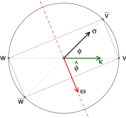
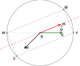
Figure 1. Elastic collision for two opposite $\sigma$’s corresponding to the two labeling of the velocities after collision. Velocities $v$ and $w$ are before collision, $\overline{v}$ and $\overline{w}$, after collision. The unit vectors are $\kappa=\widehat{v-w}$, $\sigma=\widehat{\bar{v}-\overline{w}}$, $\omega=\widehat{v-\overline{v}}=\widehat{\kappa-\sigma}$. The red dotted line represents the space generated by $\pm\omega$.The angles are given by $\cos\phi=\kappa\cdot\omega$, $\phi\in[0,\pi]$. As $\omega\cdot(\sigma+\kappa)=0$, the angles are related by $\hat{\phi}=(\pi-\phi)/2$.

We denote by $v,w\in\mathbb{R}^{3}$ the velocities before collision, while the velocities after collision are denoted by $\overline{v},\overline{w}\in\mathbb{R}^{3}$. The quadruple $(v,w,\overline{v},\overline{w})\in(\mathbb{R}^{3})^{4}$, is assumed to satisfy the conservation laws

(4) $$F_{1}(v,w,\overline{v},\overline{w}) =v+w-(\overline{v}+\overline{w})=0,$$

(5) $$F_{2}(v,w,\overline{v},\overline{w}) =\left|v\right|^{2}+\left|w\right|^{2}-(\left|\overline{v}\right|^{2}+\left|\overline{w}\right|^{2})=0,$$

which define an algebraic variety $\mathcal{M}$ that we expect to have dimension $12-(3+1)=8$. The Jacobian matrix of the four defining Eq.s (4) and (5) is

(6)   $$\kern 376.0751pt\kern-8.75pt\left[\kern-376.0751pt\vbox{\kern-42.03775pt\vbox{\halign{$#$\hfil\kern 2\p@\kern\@tempdima& \thinspace\hfil$#$\hfil&& \quad\hfil$#$\hfil\cr\hfil\crcr\kern-12.0pt\cr$\hfil\kern 2.0pt\kern 8.75pt&v_{1}&v_{2}&v_{3}&w_{1}&w_{2}&w_{3}&\overline{v}_{1}&\overline{v}_{2}&\overline{v}_{3}&\overline{w}_{1}&\overline{w}_{2}&\overline{w}_{3}\crcr\kern 2.0pt\cr\eqref{eq:momentum}_{1}$\hfil\kern 2.0pt\kern 8.75pt&1&0&0&1&0&0&-1&0&0&-1&0&0\cr\eqref{eq:momentum}_{2}$\hfil\kern 2.0pt\kern 8.75pt&0&1&0&0&1&0&0&-1&0&0&-1&0\cr\eqref{eq:momentum}_{3}$\hfil\kern 2.0pt\kern 8.75pt&0&0&1&0&0&1&0&0&-1&0&0&-1\cr\eqref{eq:energy}$\hfil\kern 2.0pt\kern 8.75pt&2v_{1}&2v_{2}&2v_{3}&2w_{1}&2w_{2}&2w_{3}&-2\overline{v}_{1}&-2\overline{v}_{2}&-2\overline{v}_{3}&-2\overline{w}_{1}&-2\overline{w}_{2}&-2\overline{w}_{3}\cr\cr}}\kern-12.0pt}\,\right]$$

The Jacobian matrix in Eq. (6) has in general position full rank, and rank 3 if $v=w=\bar{v}=\bar{w}$. We denote by $\mathcal{M}_{*}$ the 8 dimensional manifold $\mathcal{M}\setminus\left\{v=w=\overline{v}=\overline{w}\right\}$. In the sequel, for $v\neq w$, we set

$$\widehat{v-w}=\dfrac{v-w}{|v-w|}.$$

From (4) and (5) it follows the conservation of both the scalar product, $v\cdot w=\bar{v}\cdot\bar{w}$ and of the norm of the difference, $\left|v-w\right|=\left|\overline{v}-\overline{w}\right|$, so that all the vectors of the quadruple lie on a circle with center $z=(v+w)/2=(\bar{v}+\bar{w})/2$ and are the four vertexes of a rectangle. If $v=w$ then $\overline{v}=\overline{w}$, and also $v=w=\overline{v}=\overline{w}$ as the circle collapse to one point, hence we have $\mathcal{M}_{*}=\mathcal{M}\setminus\left\{v=w\right\}=\mathcal{M}\setminus\left\{\overline{v}=\overline{w}\right\}$.

There are various explicit and interesting parametrizations of $\mathcal{M}_{*}$ available.

An elementary parametrization consists of any algebraic solution of Eq.s (4) and (5) with respect to any of the free 8 coordinates. Other parametrizations are used in the literature, see classical references on the Boltzmann equation, e.g. [41].

A first parametrization is

(7) $$(u,v,\sigma)\in(\mathbb{R}^{3}\times\mathbb{R}^{3})_{*}\times\mathbb{S}^{2}\mapsto\left(u,v,\hat{A}_{\sigma}(u,v)\right)\in\mathcal{M}_{*}\subset(\mathbb{R}^{3})^{4},$$

where $\mathbb{S}^{2}=\left\{\sigma\in\mathbb{R}^{3}\middle|\,\left|\sigma\right|=1\right\}$ and the collision transformation $\hat{A}_{\sigma}\colon(v,w)\mapsto(v,w)=(v_{\sigma},w_{\sigma})$ is:

(8) $$\hat{A}_{\sigma}\colon\left\{\begin{aligned} v_{\sigma}&=\frac{v+w}{2}+\frac{\left|v-w\right|}{2}\sigma\\ w_{\sigma}&=\frac{v+w}{2}-\frac{\left|v-w\right|}{2}\sigma\end{aligned}\right..$$

Viceversa, on $\mathcal{M}_{*}$ the collision transformation depends on the unit vector $\sigma=\widehat{v-w}\in\mathbb{S}^{2}$, while the other terms depend on the collision invariants, as $\left|v-w\right|^{2}=2(\left|v\right|^{2}+\left|w\right|^{2})-\left|v+w\right|^{2}$. In conclusion, the transformation in Eq. (7) is 1-to-1 from $(\mathbb{R}^{3}\times\mathbb{R}^{3})_{*}\times\mathbb{S}^{2}$ to $\mathcal{M}_{*}$, where $(\mathbb{R}^{3}\times\mathbb{R}^{3})_{*}=\left\{(u,v)\in\mathbb{R}^{3}\times\mathbb{R}^{3}\middle|v\neq w\right\}$.

A second parametrization of $\mathcal{M}_{*}$ is obtained using the common space of two parallel sides of the velocity’s rectangle, $\operatorname{Span}\left(v-\overline{v}\right)=\operatorname{Span}\left(\overline{w}-w\right)$, so that $v-\overline{v}=\overline{w}-w=\Pi(v-w)$, where $\Pi$ is the orthogonal projection on the subspace. Viceversa, given any $\Pi$ in the set $\Pi(1)$ of projections of rank 1, the mapping

(9) $$A_{\Pi}=\begin{bmatrix}(I-\Pi)&\Pi\\ \Pi&(I-\Pi)\end{bmatrix},\quad\left\{\begin{aligned} v_{\Pi}&=v-\Pi(v-w)=(I-\Pi)v+\Pi w\\ w_{\Pi}&=w+\Pi(v-w)=\Pi v+(I-\Pi)w\end{aligned}\right..$$

The components in the direction of the image of $\Pi$ are exchanged, $\Pi v_{\Pi}=\Pi w$ and $\Pi w_{\Pi}=\Pi v$, while the orthogonal components are conserved. If $\omega$ is any of the two unit vectors such that $\Pi=\omega\otimes\omega^{\prime}$, the matrix $A_{\Pi}=A_{\omega\otimes\omega^{\prime}}$ does not depend on the direction of $\omega\in\mathbb{S}^{2}$. Notice that $A_{\Pi}^{\prime}=A_{\Pi}$ and $A_{\Pi}A_{\Pi}^{\prime}=I_{6}$, that is $A_{\Pi}$ is an orthogonal symmetric matrix. This parametrization uses the set $\Pi(1)$ of projection matrices of rank 1,

(10) $$(\mathbb{R}^{3}\times\mathbb{R}^{3})_{*}\times\Pi(1)\ni(u,v,\Pi)\mapsto\left(u,v,A_{\Pi}(u,v)\right)\in\mathcal{M}_{*}\in(\mathbb{R}^{3})^{4}\ .$$

The $\sigma$-parametrization (7) and the $\Pi$-parametrization (10) are related as follows. Given the unit vector $\kappa=\widehat{v-w}$, the parameters $\Pi$ and $\sigma$ in Eq.s (9) and (8) are in 1-to-1 relation as

(11) $$\sigma=(I-2\Pi)\kappa,\quad\Pi=\widehat{\kappa-\sigma}\otimes\widehat{\kappa-\sigma}.$$

The transition map from the parametrization (7) to the parametrization (10) is

$$(v,w,\sigma)\mapsto(v,w,(\widehat{\widehat{v-w}-\sigma})\otimes(\widehat{\widehat{v-w}-\sigma}),$$

while the inverse transition is

$$(v,w,\Pi)\mapsto(v,w,(I-2\Pi)\widehat{v-w}).$$

5.2. Uniform probabilities on $\mathbb{S}^{2}$ and on $\Pi(1)$

Let $\mu$ be the uniform probability on $\mathbb{S}^{2}$, computed, for example, in polar coordinates by

(12) $$\int_{\mathbb{S}^{2}}{f(\sigma)}\ {\mu(d\sigma)}=\frac{1}{4\pi}\int_{0}^{\pi}\sin\varphi\ d\varphi\int_{0}^{2\pi}\ f(\sin\varphi\cos\theta\ u_{1}+\sin\varphi\sin\theta\ u_{2}+\cos\varphi\ u_{3})d\theta,$$

where $u_{1},u_{2},u_{3}$ is any orthonormal basis of $\mathbb{R}^{3}$ that is $U=[u_{1}u_{2}u_{3}]\in\operatorname{SO}(3)$. In such a way, $U\colon\mathbb{S}^{2}\mapsto\mathbb{S}^{2}$ and the right hand side of Eq. (12) does not depend on $U$.

As the mapping $\omega\in\mathbb{S}^{2}\mapsto\Pi=\omega\otimes\omega\in\Pi(1)$ is a 2-covering, we define the image $\nu$ of $\mu$ by the equation

(13) $$\int_{\Pi(1)}g(\Pi)\ \nu(d\Pi)=\int_{\mathbb{S}^{2}}g(\omega\otimes\omega)\ \mu(d\omega)=2\int_{\left\{\sigma\in\mathbb{S}^{2}\middle|\kappa\cdot\sigma>0\right\}}g(\omega\otimes\omega)\ \mu(d\omega),$$

where $\kappa\in\mathbb{S}^{2}$ is any unit vector used to split $\mathbb{S}^{2}$ in two parts, $\left\{\sigma\middle|\kappa\cdot\sigma>0\right\}$ and $\left\{\sigma\middle|\kappa\cdot\sigma<0\right\}$. Eq. (13) defines a probability $\nu$ on $\Pi(1)$ such that we have the invariance

$$\int_{\Pi(1)}g(U{\Pi}U^{\prime})\ \nu(d\Pi)=\int_{\Pi(1)}g(\Pi)\ d\nu(\Pi),\quad U\in\operatorname{SO}(3).$$

Let us compute the image $T^{*}_{\kappa}\mu$ of the uniform measure $\mu$ under the action of the transformation $T_{\kappa}\colon\sigma\mapsto\omega=\widehat{\kappa-\sigma}$. If in Eq. (12) we take $u_{3}=\kappa$, that is an orthonormal basis $(u_{1},u_{2},\kappa)$, then, for $\phi,\theta$ such that $\sigma=\sin\phi\cos\theta\ u_{1}+\sin\phi\sin\theta\ u_{2}+\cos\phi\ \kappa$ and $\hat{\phi}=(\pi-\phi)/2$ (see Fig. 1) we have

$$\omega=\widehat{\kappa-\sigma} =\sin\hat{\phi}\cos\theta\ u_{1}+\sin\hat{\phi}\sin\theta\ u_{2}+\cos\hat{\phi}\ \kappa$$

$$=\sin\left(\frac{\pi-\phi}{2}\right)\cos\theta\ u_{1}+\sin\left(\frac{\pi-\phi}{2}\right)\sin\theta\ u_{2}+\cos\left(\frac{\pi-\phi}{2}\right)\ \kappa$$

(14) $$=\cos\left(\frac{\phi}{2}\right)\cos\theta\ u_{1}+\cos\left(\frac{\phi}{2}\right)\sin\theta\ u_{2}+\sin\left(\frac{\phi}{2}\right)\ \kappa$$

and for all integrable $f\colon\mathbb{R}^{3}\to\mathbb{R}$ one has

$$\int_{\mathbb{S}^{2}}{f(\omega)}\ {T^{*}_{\kappa}(d\omega)} =\int_{\mathbb{S}^{2}}{f\left(\widehat{\kappa-\sigma}\right)}\ {\mu(d\sigma)}$$

$$=\frac{1}{4\pi}\int_{0}^{\pi}\sin\phi\ d\phi\int_{0}^{2\pi}d\theta\ f\left(\cos\left(\frac{\phi}{2}\right)\cos\theta\ u_{1}+\cos\left(\frac{\phi}{2}\right)\sin\theta\ u_{2}+\sin\left(\frac{\phi}{2}\right)\ \kappa\right)$$

$$=\frac{1}{4\pi}\int_{0}^{\pi/2}2\sin(2\phi)\ d\phi\int_{0}^{2\pi}d\theta\ f\left(\cos\phi\cos\theta\ u_{1}+\cos\phi\sin\theta\ u_{2}+\sin\phi\ \kappa\right)$$

$$=\frac{1}{4\pi}\int_{0}^{\pi/2}4\cos\phi\sin(\phi)\ d\phi\int_{0}^{2\pi}d\theta\ f\left(\cos\phi\cos\theta\ u_{1}+\cos\phi\sin\theta\ u_{2}+\sin\phi\ \kappa\right)$$

(15) $$=\int_{\left\{\sigma\in\mathbb{S}^{2}\middle|\kappa\cdot\omega\geqslant 0\right\}}{f(\omega)}\ {4(\kappa\cdot\omega)\ \mu(d\omega)},$$

compare [40, 4.5].

In particular, for a symmetric function, $f(\omega)=f(-\omega)$, we have

(16) $$\int_{\mathbb{S}^{2}}{f(\omega)}\ {T^{*}_{\kappa}(d\omega)}=\int_{\mathbb{S}^{2}}{f(\widehat{\kappa-\sigma})}\ {\mu(d\sigma)}=\int_{\mathbb{S}^{2}}{f(\omega)}\ {2\left|\kappa\cdot\omega\right|\mu(d\omega)}.$$

It follows, for each integrable $g\colon\Pi(1)\to\mathbb{R}$, that

(17) $$\int_{\mathbb{S}^{2}}g((\widehat{\kappa-\sigma})\otimes(\widehat{\kappa-\sigma}))\ \mu(d\sigma)=\int_{\mathbb{S}^{2}}g(\omega\otimes\omega)\ 2\left|\kappa\cdot\omega\right|\ \mu(d\omega)$$

Notice that if we integrate Eq. (15) with respect to $\kappa$ we obtain

(18) $$\iint_{\mathbb{S}^{2}\times\mathbb{S}^{2}}f(\widehat{\kappa-\sigma})\ \mu(d\sigma)\mu(d\kappa)=\int_{\mathbb{S}^{2}}{f(\sigma)}\ {\mu(d\sigma)},$$

because

(19) $$\int_{\left\{\kappa\in\mathbb{S}^{2}\middle|\kappa\cdot\sigma\geqslant 0\right\}}{\kappa\cdot\sigma}\ {\mu(d\kappa)}=\frac{1}{4}.$$

5.3. Conditioning on the collision invariants

Given a function $g\colon\mathbb{R}^{3}\times\mathbb{R}^{3}$, Eq. (8) shows that the function

(20) $$\hat{g}\colon(u,v)\mapsto\int_{\mathbb{S}^{2}}{g(v_{\sigma},w_{\sigma})}\ {\mu(d\sigma)}=\int_{\mathbb{S}^{2}}{g\left(\hat{A}_{\sigma}(v,w)\right)}\ {\mu(d\sigma)}$$

depends on the collision invariants only. This, in turn, implies that $\hat{g}$ is the conditional expectation of $g$ with respect of the collision invariants under any probability distribution on $\mathbb{R}^{3}\times\mathbb{R}^{3}$ such that the collision invariants and the unit vector of $\sigma$ are independent, the unit vector $\sigma$ being uniformly distributed. See below a more precise statement in the case of the Gaussian distribution.

On the sample space $(\mathbb{R}^{3},dv)$, let $M$ be the standard normal density defined in (3) (the Maxwell density). As, for all $\Pi\in\Pi(1)$, $A_{\Pi}A^{\prime}_{\Pi}=A_{\Pi}A_{\Pi}=I_{6}$, in particular $\left|\det A_{\Pi}\right|=1$, we have for each $(V,W)\sim M\otimes M$ (i.e. $V,W$ are i.i.d. with distribution $M$) that

(21) $$A_{\Pi}(V,W)=(V_{\omega},W_{\omega})\sim(V,W).$$

Under the same distributions, the random variables $\frac{V+W}{\sqrt{2}}$, $\frac{\left|V-W\right|}{\sqrt{2}}$, $\widehat{V-W}$, are independent, with distributions given by

(22) $$\frac{V+W}{\sqrt{2}}\sim\text{N}\left(0_{3},I_{3}\right),\quad\frac{\left|V-W\right|^{2}}{2}\sim\chi^{2}(3),\quad\widehat{V-W}\sim\mu,$$

respectively. Hence, given any $S\sim\mu$ such that$\frac{V+W}{\sqrt{2}}$, $\frac{\left|V-W\right|}{\sqrt{2}}$, $S$, are independent, we get

(23) $$\hat{A}_{S}(V,W)\sim(V,W)\ .$$

This equality of distribution generalizes the equality of random variables $\hat{A}_{\widehat{V-W}}(V,W)=(V,W)$. We state the results obtained above as follows.

The image distribution of $M\otimes M\otimes U$ induced on $(\mathbb{R}^{3})^{4}$ by the parametrization in Eq. (7) is supported by the manifold $\mathcal{M}_{*}$. Such a distribution has the property that the projections on both the first two and the last two components are $M\otimes M$. The joint distribution is not Gaussian; in fact the support $\mathcal{M}_{*}$ is not a linear subspace. We will call this distribution the normal collision distribution.

The second parametrization in Eq. (9) shows that the variety $\mathcal{M}$ contains the bundle of linear spaces

$$(v,w)\mapsto(v,w,(I-\Pi)v+\Pi w,\Pi v+(I-\Pi)w),\quad\pi\in\Pi(1)\ .$$

The distribution of

(24) $$\mathcal{M}\ni(v,w,\bar{v},\bar{w})\mapsto\Pi=\widehat{v-\bar{v}}\otimes\widehat{v-\bar{v}}\in\Pi(1)$$

under the normal collision distribution is obtained from Eq. (11). In fact $\Pi$ is the projector on the subspace generated by $\kappa-\sigma$ where $(v,w,\sigma)\mapsto\kappa=\widehat{v-w}$ is uniformly distributed and independent from $\sigma$. Hence, Eq. (18) shows that $(v,w,\sigma)\mapsto\widehat{\kappa-\sigma}$ is uniformly distributed on $\mathbb{S}^{2}$ so that the distribution in Eq. (24) is the $\nu$ measure defined in Eq. (13). Conditionally to $\Pi$, the normal collision distribution is Gaussian with covariance

$$\begin{bmatrix}I&0&I-\Pi&\Pi\\ 0&I&\Pi&I-\Pi\\ I-\Pi&\Pi&I&0\\ \Pi&I-\Pi&0&I\end{bmatrix}\ .$$

We can give the previous remarks a more probabilistic form as follows.

Proposition 21 (Conditioning).

Let $M$ be the density of the standard normal N$(0_{3},I_{3})$ and $g\colon\mathbb{R}^{3}\times\mathbb{R}^{3}\to\mathbb{R}$ be an integrable function. It holds the following

1. If $(V,W)\sim M\otimes M$ and $\Pi\in\Pi(1)$, then

   $$\operatorname{\mathbb{E}}\left(g(V,W)\middle|V+W,\left|V\right|^{2}+\left|W\right|^{2}\right)=\operatorname{\mathbb{E}}\left(g\left(A_{\Pi}(V,W)\right)\middle|V+W,\left|V\right|^{2}+\left|W\right|^{2}\right)$$

2. If $(V,W)\sim M\otimes M$, then

   $$\int_{\mathbb{S}^{2}}{g\left(\hat{A}_{\sigma}(V,W)\right)}\ {\mu(d\sigma)}=\operatorname{\mathbb{E}}\left(g(V,W)\middle|V+W,\left|V\right|^{2}+\left|W\right|^{2}\right).$$

3. If $(V,W)\sim M\otimes M$, then

   $$2\int_{\mathbb{S}^{2}}{g\left(A_{\Pi}(V,W)\right)\left|\Pi\left(\widehat{V-W}\right)\right|}\ {\nu(d\Pi)}=\operatorname{\mathbb{E}}\left(g(V,W)\middle|V+W,\left|V\right|^{2}+\left|W\right|^{2}\right).$$

4. Assume $(V,W)\sim F$, $F\in{\mathcal{E}}\left(M\otimes M\right)$, with $F(v,w)=f(v,w)M(v)M(w)$. Then

   $$\left(\int_{\mathbb{S}^{2}}{f\circ\hat{A}_{\sigma}}\ {\mu(d\sigma)}\right)\cdot M\otimes M\in{\mathcal{E}}\left(M\otimes M\right)\ ,$$

   and

   $$\operatorname{\mathbb{E}}_{f\cdot M\otimes M}\left(g(V,W)\middle|V+W,\left|V\right|^{2}+\left|W\right|^{2}\right)=\\ \frac{\int_{\mathbb{S}^{2}}{g\left(\hat{A}_{\sigma}(V,W)\right)f\left(\hat{A}_{\sigma}(V,W)\right)}\ {\mu(d\sigma)}}{\int_{\mathbb{S}^{2}}{f\left(\hat{A}_{\sigma}(V,W)\right)}\ {\mu(d\sigma)}}=\\ \frac{\int_{\mathbb{S}^{2}}{g\left(A_{\Pi}(V,W)\right)f\left(A_{\Pi}(V,W)\right)\left|\Pi\left(\widehat{V-W}\right)\right|}\ {\nu(d\Pi)}}{\int_{\mathbb{S}^{2}}{f\left(A_{\Pi}(V,W)\right)\left|\Pi\left(\widehat{V-W}\right)\right|}\ {\nu(d\Pi)}}\ .$$

Proof.

1. We use $V+W=V_{\Pi}+W_{\Pi}$, $\left|V\right|^{2}+\left|W\right|^{2}=\left|V_{\Pi}\right|^{2}+\left|W_{\Pi}\right|^{2}$, $(V,W)\sim(V_{\Pi},W_{\Pi})$. For all bounded $h_{1}\colon\mathbb{R}^{3}\to\mathbb{R}$ and $h_{2}\colon\mathbb{R}\to\mathbb{R}$, we have

   $$\operatorname{\mathbb{E}}\left(\operatorname{\mathbb{E}}\left(g\left(A_{\Pi}(V,W)\right)\middle|V+W,\left|V\right|^{2}+\left|W\right|^{2}\right)h_{1}(V+W)h_{2}(\left|V\right|^{2}+\left|W\right|^{2})\right)=\\ \operatorname{\mathbb{E}}\left(g(V_{\Pi},W_{\Pi})h_{1}(V+W)h_{2}(\left|V\right|^{2}+\left|W\right|^{2})\right)=\\ \operatorname{\mathbb{E}}\left(g(V_{\omega},W_{\omega})h_{1}(V_{\Pi}+W_{\Pi})h_{2}(\left|V_{\omega}\right|^{2}+\left|W_{\omega}\right|^{2})\right)=\\ \operatorname{\mathbb{E}}\left(g(V,W)h_{1}(V+W)h_{2}(\left|V\right|^{2}+\left|W\right|^{2})\right)=\\ \operatorname{\mathbb{E}}\left(\operatorname{\mathbb{E}}\left(g(V,W)\middle|V+W,\left|V\right|^{2}+\left|W\right|^{2}\right)h_{1}(V+W)h_{2}(\left|V\right|^{2}+\left|W\right|^{2})\right).$$

2. For a generic integrable $h\colon\mathbb{R}^{3}\times\mathbb{R}^{3}\to\mathbb{R}$ we have

   $$\operatorname{\mathbb{E}}\left(h(V,W)\right)=\\ \operatorname{\mathbb{E}}\left(h\left(\frac{V+W}{2}+\frac{\left|V-W\right|}{2}\widehat{V-W},\frac{V+W}{2}-\frac{\left|V-W\right|}{2}\widehat{V-W}\right)\right)=\\ \int_{\mathbb{S}^{2}}\operatorname{\mathbb{E}}\left(h\left(\frac{V+W}{2}+\frac{\left|V-W\right|}{2}\sigma,\frac{V+W}{2}-\frac{\left|V-W\right|}{2}\sigma\right)\right)\ \mu(d\sigma)=\\ \int_{\mathbb{S}^{2}}\operatorname{\mathbb{E}}\left(h(\hat{A}_{\sigma}(V,W))\right)\ \mu(d\sigma)\ ,$$

   because $\widehat{V-W}\sim\mu$, and $(V+W)$, $\left|V-W\right|$, $\widehat{V-W}$ are independent.

   The random variable

   $$\int_{\mathbb{S}^{2}}{g\circ\hat{A}_{\sigma}(V,W)}\ {\mu(d\sigma)}=\int_{\mathbb{S}^{2}}{g\left(\frac{V+W}{2}+\frac{\left|V-W\right|}{2}\sigma,\frac{V+W}{2}-\frac{\left|V-W\right|}{2}\sigma\right)}\ {\mu(d\sigma)}$$

   is a function of the collision invariants i.e., it is of the form $\tilde{g}(V+W,\left|V\right|^{2}+\left|W\right|^{2})$. For all bounded $h_{1}\colon\mathbb{R}^{3}\to\mathbb{R}$ and $h_{2}\colon\mathbb{R}\to\mathbb{R}$, we apply the previous computation to $h=gh_{1}h_{2}$ to get

   $$\operatorname{\mathbb{E}}\left(\left(\int_{\mathbb{S}^{2}}{g\circ\hat{A}_{\sigma}(V,W)}\ {\mu(d\sigma)}\right)h_{1}(V+W)h_{2}(\left|V\right|^{2}+\left|W\right|^{2})\right)=\\ \int_{\mathbb{S}^{2}}{\operatorname{\mathbb{E}}\left(g\circ\hat{A}_{\sigma}(V,W)h_{1}(V+W)h_{2}(\left|V\right|^{2}+\left|W\right|^{2})\right)}\ {\mu(d\sigma)}=\\ \int_{\mathbb{S}^{2}}{\operatorname{\mathbb{E}}\left(g\circ\hat{A}_{\sigma}(V,W)h_{1}(V_{\sigma}+W_{\sigma})h_{2}(\left|V_{\sigma}\right|^{2}+\left|W_{\sigma}\right|^{2})\right)}\ {\mu(d\sigma)}=\\ \operatorname{\mathbb{E}}\left(g(V,W)h_{1}(V+W)h_{2}(\left|V\right|^{2}+\left|W\right|^{2})\right).$$

3. We use Item 2 and the equality $\hat{A}_{\sigma}(v,w)=A_{\Pi}(v,w)$ when $\Pi=\widehat{\kappa-\sigma}\otimes\widehat{\kappa-\sigma}$ and $\kappa=\widehat{v-w}$ to write

   $$\int_{\mathbb{S}^{2}}{g\left(A_{{\widehat{V-W}-\sigma}\widehat{\otimes}{\widehat{V-W}-\sigma}}(V,W)\right)}\ {\mu(d\sigma)}=\operatorname{\mathbb{E}}\left(g(V,W)\middle|V+W,\left|V\right|^{2}+\left|W\right|^{2}\right)$$

   where, for given vectors $u,v\in\mathbb{R}^{3}$, $u,v\neq 0$ we simply denote $u\,\widehat{\otimes}\,v=\widehat{u}\otimes\widehat{v}.$ From Eq. (17), the left-end-side can be rewritten as an integral with respect to $\omega\in\mathbb{S}^{2}$,

   $$\int_{\mathbb{S}^{2}}{g\left(A_{\omega\otimes\omega}(V,W)\right)2\left|\widehat{V-W}\cdot\omega\right|}\ {\mu(d\omega)}=\int_{\mathbb{S}^{2}}{g\left(A_{{\widehat{V-W}-\sigma}\widehat{\otimes}{\widehat{V-W}-\sigma}}(V,W)\right)}\ {\mu(d\sigma)}\ .$$

   If $\Pi=\omega\otimes\omega$, then $\left|\kappa\cdot\omega\right|=\left|\omega\otimes\omega\kappa\right|=\left|\Pi\kappa\right|$. Using that together with the definition of the measure $\nu$ on $\Pi(1)$ in Eq. (13), we have the result:

   $$\int_{\mathbb{S}^{2}}{g\left(A_{\omega\otimes\omega}(V,W)\right)2\left|\widehat{V-W}\cdot\omega\right|}\ {\mu(d\omega)}=\\ \int_{\mathbb{S}^{2}}{g\left(A_{\omega\otimes\omega}(V,W)\right)2\left|(\omega\otimes\omega)\widehat{V-W}\right|}\ {\mu(d\omega)}=\\ 2\int_{\Pi(1)}{g\left(A_{\Pi}(V,W)\right)\left|\Pi(\widehat{V-W})\right|}\ {\nu(d\Pi)}.$$

4. We use Th. 8. If $F\in{\mathcal{E}}\left(M\otimes M\right)$, then

   $$F=\mathrm{e}^{U-K_{M\otimes M}(U)}M\otimes M,\quad U\in\mathcal{S}_{M\otimes M}\ ,$$

   and there exists a neighborhood $I$ of $[0,1]$, where the one dimensional exponential family

   $$F_{t}=\mathrm{e}^{tU-K_{0}(tM)}M\otimes M,\quad t\in I,$$

   exists. The random variable

   (25) $$\hat{f}=\int_{\mathbb{S}^{2}}{f\circ\hat{A}_{\sigma}}\ {\mu(d\sigma)}$$

   is a positive probability density with respect to $M\otimes M$ because it is the conditional expectation in $M\otimes M$ of the positive density $f$.

   In order to show that ${\operatorname{\mathbb{E}}}_{M\otimes M}\left[(\hat{f})^{t}\right]<+\infty$ for $t\in I$, it is enough to consider the convex cases, $t<0$ and $t>1$, because otherwise ${\operatorname{\mathbb{E}}}_{M\otimes M}\left[(\hat{f})^{t}\right]\leqslant 1$. We have

   $$\int_{\mathbb{S}^{2}}{f\circ\hat{A}_{\sigma}}\ {\mu(d\sigma)}=\int_{\mathbb{S}^{2}}{\mathrm{e}^{U\circ\hat{A}_{\sigma}-K_{M\otimes M}(U)}}\ {\mu(d\sigma)}\ ,$$

   so that in the convex cases:

   $${\operatorname{\mathbb{E}}}_{M\otimes M}\left[\left(\int_{\mathbb{S}^{2}}{f\circ\hat{A}_{\sigma}}\ {\mu(d\sigma)}\right)^{t}\right]={\operatorname{\mathbb{E}}}_{M\otimes M}\left[\left(\int_{\mathbb{S}^{2}}{\mathrm{e}^{U\circ\hat{A}_{\sigma}-K_{M\otimes M}(U)}}\ {\mu(d\sigma)}\right)^{t}\right]\leqslant\\ {\operatorname{\mathbb{E}}}_{M\otimes M}\left[\int_{\mathbb{S}^{2}}{\mathrm{e}^{tU\circ\hat{A}_{\sigma}-tK_{M\otimes M}(U)}}\ {\mu(d\sigma)}\right]={\operatorname{\mathbb{E}}}_{M\otimes M}\left[\mathrm{e}^{tU-tK_{M\otimes M}(U)}\right]=\\ \mathrm{e}^{K_{M\otimes M}(tU)-tK_{M\otimes M}(U)}<+\infty,\quad t\in I\setminus[0,1].$$

   To conclude, use Bayes’ formula for conditional expectation,

   $$\operatorname{\mathbb{E}}_{f\cdot M\otimes M}\left(A\middle|\mathcal{B}\right)=\frac{\operatorname{\mathbb{E}}_{M\otimes M}\left(Af\middle|\mathcal{B}\right)}{\operatorname{\mathbb{E}}_{M\otimes M}\left(f\middle|\mathcal{B}\right)}\ .$$

   to the expressions of conditional expectation in Item 2 and Item 3 above.

∎

Remark 4.

In the last Item, we compute a conditional expectation of a density $f$, that is

$$\operatorname{\mathbb{E}}\left(f(V,W)\middle|V+W,\left|V\right|^{2}+\left|W\right|^{2}\right)=\hat{f}(V+W,\left|V\right|^{2}+\left|W\right|^{2}).$$

The random variable $\hat{f}\colon\mathbb{R}^{3}\times\mathbb{R}_{+}\to\mathbb{R}$ is the density of the image of $F\ dvdw$ with respect to the image of $M(v)M(w)\ dvdw$.

5.4. Interactions

We introduce here the crucial role played by microscopic interaction in the definition of the Boltzmann collision operator. In the physics literature, such interaction are referred to as the kinetic collision kernel and takes into account the intermolecular forces suffered by particles during a collision [41]. Before defining formally what we mean by interaction, we first observe that, if $M$ is the Maxwell density on $\mathbb{R}^{3}$ and $f,g\smile M$ then

$$f\otimes g\smile M\otimes M$$

where $M\otimes M$ is the standard normal density on $\mathbb{R}^{6}$ and $f\otimes g$ is a density on $\mathbb{R}^{6}$. Indeed, one has

$$f(v) =\mathrm{e}^{U(v)-K_{M}(U)}M(v),\quad U\in\mathcal{S}_{M}\ ,$$

$$g(w) =\mathrm{e}^{V(w)-K_{M}(V)}M(w),\quad V\in\mathcal{S}_{M}\ .$$

It follows that the product density has the form

$$f(v)g(w)=\mathrm{e}^{U(v)+V(w)-K_{M}(U)-K_{M}(V)}M(v)M(w),\quad U\oplus V\in\mathcal{S}_{M}\otimes\mathcal{S}_{M}\subset\mathcal{S}_{M\otimes M}\ ,$$

which implies $f\otimes g\smile M\otimes M$, with $K_{M\otimes M}(U\oplus V)=K_{M}(U)+K_{M}(V)$.

Definition 22.

With the previous notations, we say that $b\colon\mathbb{R}^{3}\times\mathbb{R}^{3}\to\mathbb{R}^{+}$ is an interaction on ${\mathcal{E}}\left(M\right)\otimes{\mathcal{E}}\left(M\right)$, if ${\operatorname{\mathbb{E}}}_{f\otimes g}\left[b\right]<+\infty$, so that

$$\frac{b}{{\operatorname{\mathbb{E}}}_{f\otimes g}\left[b\right]}f\otimes g\colon(v,w)\in\mathbb{R}^{3}\times\mathbb{R}^{3}\mapsto\frac{b(v,w)}{{\operatorname{\mathbb{E}}}_{f\otimes g}\left[b\right]}f(v)g(w)$$

is a density.

Sometimes, we make the abuse of notation by writing ${\operatorname{\mathbb{E}}}_{b\cdot f\otimes g}\left[\cdot\right]$, where the obvious normalization is not written down. As can been seen, here interactions indicate only a class of suitable weight functions $b$ for which $b(v,w)f(v)g(w)$ is still (up to normalisation) a density. This is in accordance with the usual role played by the kinetic collision kernel (see [41]).

According to the Portmanteau Theorem 8, it holds $\frac{b}{{\operatorname{\mathbb{E}}}_{f\otimes g}\left[b\right]}\cdot f\otimes g\smile M\otimes M$ if and only if $\frac{b}{{\operatorname{\mathbb{E}}}_{f\otimes g}\left[b\right]}\cdot f\otimes g\smile f\otimes g$, which, in turn, is equivalent to ${\operatorname{\mathbb{E}}}_{f\otimes g}\left[b^{1+\epsilon}\right],{\operatorname{\mathbb{E}}}_{b\cdot f\otimes g}\left[b^{-1-\epsilon}\right]<\infty$ for some $\epsilon>0$.

Proposition 23.

Let $b\colon\mathbb{R}^{3}\times\mathbb{R}^{3}\to\mathbb{R}^{+}$ be such that for some real $A\in\mathbb{R}$ and positive $B,C,\lambda\in\mathbb{R}_{>}$, it holds

$$C\left|u-v\right|^{\lambda}\leqslant b(u,v)\leqslant A+B\left|u-v\right|^{2}\ .$$

Then the $b$ is an interaction on ${\mathcal{E}}\left(M\right)\times{\mathcal{E}}\left(M\right)$ and for all $f,g\smile M$ the following holds.

1. $\frac{b}{{\operatorname{\mathbb{E}}}_{f\otimes g}\left[b\right]}\cdot f\otimes g\smile M\otimes M$.

2. Assume moreover that the interaction $b$ is a function of the invariants only

   $$b(v,w)=\hat{b}(v+w,\left|v\right|^{2}+\left|w\right|^{2})\ .$$

   It follows

   $$\operatorname{\mathbb{E}}_{M\otimes M}\left(b\cdot f\otimes g\middle|V+W,\left|V\right|^{2}+\left|W\right|^{2}\right)=b(V,W)\int_{\mathbb{S}^{2}}{f\otimes g\circ\hat{A}_{\sigma}(V,W)}\ {\mu(d\sigma)}\ .$$

   and moreover a sufficiency relation holds i.e., for all integrable $F\colon\mathbb{R}^{3}\times\mathbb{R}^{3}\to\mathbb{R}$, it holds

   $$\operatorname{\mathbb{E}}_{b\cdot f\otimes g}\left(F(V,W)\middle|V+W,\left|V\right|^{2}+\left|W\right|^{2}\right)=\operatorname{\mathbb{E}}_{f\otimes g}\left(F(V,W)\middle|V+W,\left|V\right|^{2}+\left|W\right|^{2}\right)\ .$$

Proof.

1. We can assume ${\operatorname{\mathbb{E}}}_{f\otimes g}\left[b\right]=1$. As $b(u,v)\leqslant A+B\left|u-v\right|^{2}\leqslant A+2B\left|(u,v)\right|^{2}$, we have $b\in L^{\Phi}(M\otimes M)=L^{\Phi}(f\otimes g)$, and hence $b\in L^{1+\epsilon}(f\otimes g)$ for all $\epsilon>0$. For the second inequality we use the Hardy-Littlewood-Sobolev inequality [25, Th. 4.3]. We have

$${\operatorname{\mathbb{E}}}_{b\cdot f\otimes g}\left[b^{-1-\epsilon}\right]=\iint\frac{f(u)g(v)}{b(u,v)^{\epsilon}}\ dudv\leqslant C^{-1}\iint\frac{f(u)g(v)}{\left|u-v\right|^{\epsilon\lambda}}\ dudv.$$

If $\frac{1}{\beta}+\frac{\epsilon\lambda}{3}+\frac{1}{\alpha}=2$, by the H-L-S inequality the last integral is bounded by a constant times $\left\|f\right\|_{\alpha}\left\|g\right\|_{\beta}$. From $f,g\smile M$ we get that $\left\|f\right\|_{\alpha}\left\|g\right\|_{\beta}$ is finite for $\alpha,\beta$ in a right neighborhood of 1. There exists $\epsilon=\frac{3}{\lambda}\left(2-\frac{1}{\alpha}-\frac{1}{\beta}\right)>0$ satisfying all conditions.

2. It is a special case of the Conditioning Theorem 21. ∎

Let us discuss the differentiability of the operations we have just introduced.

Proposition 24.

1. The product mapping ${\mathcal{E}}\left(M\right)\ni f\mapsto f\otimes f$ is a differentiable map into ${\mathcal{E}}\left(M\otimes M\right)$ with tangent mapping given for any vector field $X\in T{\mathcal{E}}\left(M\right)$ by

   $$T_{f}{\mathcal{E}}\left(M\right)\ni X_{f}\mapsto X_{f}\oplus X_{f}\in T_{f\otimes f}{\mathcal{E}}\left(M\otimes M\right)\ .$$

2. Let $b$ be an interaction on ${\mathcal{E}}\left(M\right)\otimes{\mathcal{E}}\left(M\right)$. If the mapping

   $$f\mapsto\frac{b}{{\operatorname{\mathbb{E}}}_{f\otimes f}\left[b\right]}\cdot f\otimes f$$

   is defined on ${\mathcal{E}}\left(M\right)$ with values in ${\mathcal{E}}\left(M\otimes M\right)$, then it is differentiable with tangent mapping given for all vector field $X\in T{\mathcal{E}}\left(M\right)$ by

   $$X_{f}\mapsto X_{f}\oplus X_{f}-{\operatorname{\mathbb{E}}}_{b\cdot f\otimes f}\left[X_{f}\oplus X_{f}\right]\ .$$

Proof.

1. We have already proved that $f\smile M$ implies $f\otimes f\smile M\otimes M$ and that the mapping in the charts centered at $M$ and $M\otimes M$ respectively is represented as $\mathcal{S}_{M}\ni U\mapsto U+U\in\mathcal{S}_{M\otimes M}$. The differential of the linear map is again $T_{M}{\mathcal{E}}\left(M\right)\ni V\mapsto V\oplus V\in T_{M\otimes M}{\mathcal{E}}\left(M\otimes M\right)$. The transport commutes with the $\oplus$ operation,

   $$\mathbb{U}_{M\otimes M}^{f\otimes f}\left(V\oplus V\right)=\left(\mathbb{U}_{M}^{f}V\right)\oplus\left(\mathbb{U}_{M}^{f}V\right)\ ,$$

   and the result follows.

2. Let $U$ be the coordinate of $f$ at $M$. By assumption, we have

   $$\frac{b}{{\operatorname{\mathbb{E}}}_{f\otimes f}\left[b\right]}\cdot f\otimes f\smile\frac{b}{{\operatorname{\mathbb{E}}}_{M\otimes M}\left[b\right]}\cdot M\otimes M$$

   and

   $$\frac{\frac{b}{{\operatorname{\mathbb{E}}}_{f\otimes f}\left[b\right]}\cdot f\otimes f}{\frac{b}{{\operatorname{\mathbb{E}}}_{M\otimes M}\left[b\right]}\cdot M\otimes M}=\frac{{\operatorname{\mathbb{E}}}_{M\otimes M}\left[b\right]}{{\operatorname{\mathbb{E}}}_{f\otimes f}\left[b\right]}\exp\left(U\oplus U-2K_{M}(U)\right)\ ,$$

   so that the coordinate of $\frac{b}{{\operatorname{\mathbb{E}}}_{f\otimes f}\left[b\right]}\cdot f\otimes f$ in the chart centered at $\frac{b}{{\operatorname{\mathbb{E}}}_{M\otimes M}\left[b\right]}\cdot M\otimes M$ is

   $$U\oplus U-{\operatorname{\mathbb{E}}}_{b\cdot M\otimes M}\left[U\oplus U\right]=\mathbb{U}_{M\otimes M}^{b\cdot M\otimes M}(U\oplus U).$$

   The expression if linear and so is the expression of the tangent map

   $$V\mapsto V\oplus V-{\operatorname{\mathbb{E}}}_{b\cdot M\otimes M}\left[V\oplus V\right]\ .$$

   In conclusion, for each vector field $X$ of $T{\mathcal{E}}\left(M\right)$, at $f$ we have $V=\mathbb{U}_{f}^{M}X_{f}$ and $V\oplus V=\mathbb{U}_{f\oplus f}^{M\oplus M}(X_{f}\oplus X_{f})$, hence the action on $T_{f}{\mathcal{E}}\left(M\right)$ is as stated.

∎

Assume $f\smile M$ and let $b$ be an interaction on $f\otimes f$ which depends on the invariants only and such that $b\cdot f\otimes f\smile M\otimes M$. For each random variable $g\in L^{\cosh-1}(M)=L^{\cosh-1}(f)$, define $\overline{g}=\frac{1}{2}\ g\oplus g$, which belongs to $L^{\cosh-1}(M\otimes M)=L^{\cosh-1}(f\otimes f)$. Define the operator

$$A\colon L^{\cosh-1}(M)\to L^{\cosh-1}(M\otimes M)\ ,$$

by

$$Ag(v,w)=\int_{\mathbb{S}^{2}}{\overline{g}\left(\hat{A}_{\sigma}(v,w)\right)}\ {\mu(d\sigma)}-\overline{g}(V,W)\ .$$

As constant random variables are in the kernel of the operator $A$, we assume ${\operatorname{\mathbb{E}}}_{f}\left[g\right]=0$.

5.5. Maxwell-Boltzmann and Boltzmann operator

As explained by C. Villani [41, I.2.3], Maxwell obtained a weak form of Boltzmann operator before Boltzmann himself. We rephrase in geometric-probabilistic language such a Maxwell’s weak form by expanding and rigorously proving what was hinted to in [33].

Let $b\colon\mathbb{R}^{3}\times\mathbb{R}^{3}\to\mathbb{R}^{+}$ be an interaction on ${\mathcal{E}}\left(M\right)\times{\mathcal{E}}\left(M\right)$ which depends on the invariants only and such that $b\cdot f\otimes f\smile M\otimes M$ if $f\smile M$, cf. Prop. 23. We shall call such a $b$ a proper interaction.

For each random variable $g\in L^{\cosh-1}(M)=L^{\cosh-1}(f)$, define $\overline{g}=\frac{1}{2}\ g\oplus g$ by

$$\overline{g}(v,w)=\frac{1}{2}\left(g(v)+g(w)\right)$$

which it is easily shown to belong to $L^{\cosh-1}(M\otimes M)=L^{\cosh-1}(f\otimes f)$. The mapping $g\mapsto\overline{g}$ is a version of the conditional expectation $\operatorname{\mathbb{E}}_{M\otimes M}\left(g\middle|\mathcal{S}\right)$, where $\mathcal{S}$ is the $\sigma$-algebra generated by symmetric random variables.

We define the operator

$$A\colon L^{\cosh-1}(M)\to L^{\cosh-1}(M\otimes M)\ ,$$

by

$$Ag(v,w)=\int_{\mathbb{S}^{2}}{\overline{g}\left(\hat{A}_{\sigma}(v,w)\right)}\ {\mu(d\sigma)}-\overline{g}(V,W)\ ,$$

which is a version of

$$Ag=\operatorname{\mathbb{E}}_{M\otimes M}\left(\operatorname{\mathbb{E}}_{M\otimes M}\left(g\middle|\mathcal{S}\right)\middle|\mathcal{I}\right)-\operatorname{\mathbb{E}}_{M\otimes M}\left(g\middle|\mathcal{S}\right)=\operatorname{\mathbb{E}}_{M\otimes M}\left(g\middle|\mathcal{I}\right)-\operatorname{\mathbb{E}}_{M\otimes M}\left(g\middle|\mathcal{S}\right)\ ,$$

where $\mathcal{I}\subset\mathcal{S}$ is the $\sigma$-algebra generated by the collision invariants $(v,w)\mapsto(v+w,\left|v\right|^{2}+\left|w\right|^{2})$.

As constant random variables are in the kernel of the operator $A$, we assume ${\operatorname{\mathbb{E}}}_{f}\left[g\right]=0$. Analogously, as the kernel of the operator contains all symmetric random variables, we could always assume that $g$ is anti-symmetric.

The nonlinear operator $f\mapsto{\operatorname{\mathbb{E}}}_{b\cdot f\otimes f}\left[Ag\right]$ is the Maxwell’s weak form of the Boltzmann operator, $g$ being a test function.

Proposition 25.

Given a proper interaction $b$ and a density $f\in{\mathcal{E}}\left(M\right)$, the linear map

$$L_{0}^{\cosh-1}(M)\ni g\mapsto{\operatorname{\mathbb{E}}}_{b\cdot f\otimes f}\left[Ag\right]$$

is continuous.

1. It can be represented in the duality $L^{(\cosh-1)_{*}}(f)\times L^{\cosh-1}(f)$ by

   $${\operatorname{\mathbb{E}}}_{b\cdot f\otimes f}\left[Ag\right] ={\operatorname{\mathbb{E}}}_{M\otimes M}\left[b\left(\operatorname{\mathbb{E}}_{M\otimes M}\left(\frac{f}{M}\otimes\frac{f}{M}\middle|\mathcal{I}\right)-\frac{f}{M}\otimes\frac{f}{M}\right)g\right]$$

   $$=\left\langle Q(f)/f,g\right\rangle_{f}\ ,$$

   where $Q$ is the Boltzmann operator with interaction $b$,

   $$Q(f)(v)=\int_{\mathbb{R}^{3}}\int_{\mathbb{S}^{2}}\left(f\otimes f\left(\hat{A}_{\sigma}(v,w)\right)-f(v)f(w)\right)b(v,w)\ \mu(d\sigma)\ dw$$

2. Especially, if $f=\mathrm{e}^{U-K_{M}(U)}M$ and we take $g=\log\left(\frac{f}{M}\right)$, then

   $${\operatorname{\mathbb{E}}}_{b\cdot f\otimes f}\left[A\log\left(\frac{f}{M}\right)\right]=\left\langle Q(f)/f,U\right\rangle_{f}\ .$$

Proof.

The continuity follows from the Portmanteau theorem and the continuity of the conditional expectation. Item 1 follows from the projection properties of the conditional expectation and from general properties of Orlicz spaces. Item 2 is a special case of the previous one. ∎

It follows from the previous theorem and from the discussion in [33, Prop. 10] that $f\mapsto Q(f)/f$ is a vector field in the cotangent bundle $\prescript{*}{}{T}{\mathcal{E}}\left(M\right)$ and its flow

$$\frac{D}{dt}f_{t}=\frac{\dot{f}_{t}}{f_{t}}=\frac{Q(f_{t})}{f_{t}}$$

is equivalent to the standard Boltzmann equation $\dot{f}_{t}=Q(t)$. We do not discuss in this paper the implications of that presentation of the Boltzmann equation to the existence properties. We turn our attention to the comparison of the Boltzmann field to the gradient field of the entropy.

5.6. Entropy generation

If $t\mapsto p(t)$ is a curve in ${\mathcal{E}}\left(M\right)$, the entropy of $p(t)$ is defined for all $t$ and the variation of the entropy along the curve is computed as

$$\frac{d}{dt}H(p_{t})=-\int\frac{d}{dt}\left(p(v;t)\log p(v;t)\right)\ dv=\\ -\int\left(\log p(v;t)-1\right)\frac{d}{dt}p(v;t)\ dv=-\int\log p(v;t)\frac{d}{dt}p(v;t)\ dv\ .$$

In our setup, the computation takes the following form. Let $t\mapsto p_{t}$ be a differentiable curve in ${\mathcal{E}}\left(M\right)$ with velocity $t\mapsto Dp_{t}\in\prescript{*}{}{B}_{p_{t}}$. As the gradient $\nabla H$ is given at $p$ by $(\nabla H)(p)=-(\log p+H(p))\in B_{p}$, we have

$$\frac{d}{dt}H(p(t))=-\left\langle\log p(t)+H(p(t)),Dp(t)\right\rangle_{p(t)}\ .$$

In particular, if $Dp(t)=\dot{p}(v;t)/p(v;t)$ we recover the previous computation:

$$\frac{d}{dt}H(p(t)) =-\int\left(\log p(t)+H(p(t))\right)\frac{\dot{p}(v;t)}{p(v;t)}\ p(v;t)dv$$

$$=-\int\log p(v;t)\frac{d}{dt}p(v;t)\ dv\ .$$

Assume now that $(p,t)\mapsto\gamma(t;p)$ is the flow of a vector field $F\colon{\mathcal{E}}\left(M\right)\to\prescript{*}{}{T}{\mathcal{E}}\left(M\right)$. Then

$$\frac{d}{dt}H(\gamma(t;p)) =-\left\langle\log\gamma(t;p)+H(\gamma(t;p)),D\gamma(t;p)\right\rangle_{\gamma(t;p)}$$

$$=-\left\langle\log\gamma(t;p)+H(\gamma(t;p)),F(\gamma(t;p))\right\rangle_{\gamma(t;p)},$$

that is, for each $p\in{\mathcal{E}}\left(M\right)$, the entropy production at $p$ along the vector field $F$ is

$$(\nabla_{F}H)(p)=-\left\langle\log p+H(p),F(p)\right\rangle_{p}=\\ -\int\left(\log p(v)+H(p)\right)F(v,p)\ p(x)dx=-\int\log p(v)F(v,p)\ p(v)dv\ .$$

In particular, if the vector field $F$ is the Boltzmann vector field, $F(f)=Q(f)/f$, we have that for each $f\in{\mathcal{E}}\left(M\right)$ the Boltzmann’s entropy production is

$$\operatorname{\mathscr{D}}\left(f\right)=(\nabla_{Q(f)/f}H)(f)=-\left\langle\log f+H(f),Q(f)/f\right\rangle_{f}\\ =-{\operatorname{\mathbb{E}}}_{b\cdot f\otimes f}\left[A\log f\right]=-\frac{1}{2}{\operatorname{\mathbb{E}}}_{b\cdot f\otimes f}\left[A\left(\log f\ominus\log f\right)\right]\ ,$$

where

$$\left(\log f\ominus\log f\right)(v,w)=\log f(v)-\log f(w)=\log\frac{f(v)}{f(w)}\ .$$

We recover a well-known formula for the entropy production of the Boltzmann operator [41]. We now proceed to compute the covariant derivative of the entropy production.

Proposition 26.

Let $X$ be a vector field of $T{\mathcal{E}}\left(M\right)$ and let $F$ be a vector field of $\prescript{*}{}{T}{\mathcal{E}}\left(M\right)$.

1. The Hessian of the entropy (in the exponential connection) is

   $$D_{X}\nabla H(f)=-X.$$

2. The covariant derivative of the entropy production along $F$ is

   $$D_{X}\operatorname{\mathscr{D}}=-\left\langle X,F\right\rangle+\left\langle\nabla H,D_{X}F\right\rangle.$$

Proof.

We note that the entropy production along a vector field $F$, $\operatorname{\mathscr{D}}=(\nabla_{F}H)(p)=\left\langle\nabla H,F\right\rangle$, is a function of the duality coupling of $T{\mathcal{E}}\left(M\right)\times\prescript{*}{}{T}{\mathcal{E}}\left(M\right)$, so that we can apply Prop. 16 to compute its covariant derivative along $X$ as

$$D_{X}\operatorname{\mathscr{D}}=\left\langle D_{X}\nabla H,F\right\rangle+\left\langle\nabla H,D_{X}F\right\rangle.$$

The first term at $p$ is

$$\left\langle D_{X}\nabla H,F\right\rangle(p)=\left\langle D_{X}\nabla H(p),F(p)\right\rangle_{p}.$$

Let us compute $D_{X}\nabla H(p)$, which is the Hessian of the entropy in the exponential connection. First, we compute the expression of $\nabla H(q)=-\left(\log q+H(q)\right)\in B_{q}$, $q\in{\mathcal{E}}\left(M\right)$ in the chart centered at $p$. We have

$$-\log q=K_{p}(U)-U-\log p,\quad U\in\mathcal{S}_{p},q=e_{p}(U),$$

and

$$H_{p}(U)=-{\operatorname{\mathbb{E}}}_{q}\left[\log q\right]=K_{p}(U)-dK_{p}(U)[U]+dK_{p}(U)[\nabla H(p)]+H(p)$$

so that

$$(\nabla H)\circ e_{p}(U)=-U+dK_{p}(U)[U]+\nabla H(p)-dK_{p}(U)[\nabla H(p)]$$

and, finally, the expression of $\nabla H$ in the chart centered at $p$ is

$$(\nabla H)_{p}(U)=\prescript{\text{e}}{}{\mathbb{U}}_{e_{p}(U)}^{p}(\nabla H)\circ e_{p}(U)=\nabla H(p)-U.$$

Note that this function is affine, and its derivative in the direction $X(p)$ is $d(\nabla H)_{p}(U)[X(p)]=-X(p)$. It follows that $D_{X}\nabla H=-X$. ∎

The application of this computation to the Boltzmann field i.e. $F(f)=Q(f)/f$ requires the existence of the covariant derivative of the Boltzmann operator. We leave this discussion as a research plan.

6. Weighted Orlicz-Sobolev model space

We show in this section that the Information Geometry formalism described in Sections 2 and 3 is robust enough to allow to take into account differential operators (e.g., the classical Laplacian). This yields naturally to the introduction of weighted Orlicz-Sobolev spaces. While the case “without derivative” studied in Section 3 was well-suited for the study of the fine properties of the Kullback-Leibler divergence, we illustrate in Sec. 6.3 our use of Orlicz-Sobolev spaces with the fine study of the Hyvärinen divergence. This is a special type of divergence between densities that involves an $L^{2}$-distance between gradients of densities [21] which has multiple applications. In particular, it is related with the so called Fisher information as it is defined for example in [40, p. 49], which has deep connections with Boltzmann equation, see [39]. However the name Fisher information should not be used in a statistics context where it rather refers to the expression in coordinates of the metric of statistical models considered as pseudo-Riemannian manifolds e.g., [4].

We introduce the Orlicz-Sobolev spaces with weight $M$, Maxwell density on $\mathbb{R}^{n}$,

(26) $$W_{\cosh-1}^{1}(M)=\left\{f\in L^{\cosh-1}\left(M\right)\middle|\partial_{j}f\in L^{\cosh-1}\left(M\right),j=1,\dots,n\right\},$$

(27) $$W_{(\cosh-1)_{*}}^{1}(M)=\left\{f\in L^{(\cosh-1)_{*}}\left(M\right)\middle|\partial_{j}f\in L^{(\cosh-1)_{*}}\left(M\right),j=1,\dots,n\right\},$$

where $\partial_{j}$ is the derivative in the sense of distributions. They are both Banach spaces, see [28, §10]. (The classical Adams’s treatise [2, Ch 8] has Orlicz-Sobolev spaces, but does not consider the case of a weight. The product functions $(u,x)\mapsto(\cosh-1)(u)M(x)$ and $(u,x)\mapsto(\cosh-1)_{*}(u)M(x)$ are $\phi$-functions according the Musielak’s definition.) The norm on $W_{\cosh-1}^{1}(M)$ is

(28) $$\left\|f\right\|_{W^{1}_{\cosh-1}(M)}=\left\|f\right\|_{L^{\cosh-1}\left(M\right)}+\sum_{j=1}^{n}\left\|\partial_{j}f\right\|_{L^{\cosh-1}\left(M\right)},$$

and similarly for $W^{1}_{(\cosh-1)_{*}}(M)$. One begins with a first technical result in order to relate such spaces with statistical exponential families:

Proposition 27.

Given $u\in\mathcal{S}_{M}\cap W^{1}_{\cosh-1}(M)$ and $f\in W^{1}_{\cosh-1}(M)$, one has

$$f\mathrm{e}^{u-K_{M}(u)}\in W^{1}_{(\cosh-1)_{*}}(M).$$

Proof.

For simplicity, set $G=\mathrm{e}^{u-K_{M}(u)}.$ One knows from the Portmanteau Theorem 8 that $G\,M\in{\mathcal{E}}\left(M\right)$ and therefore, there exists $\varepsilon>0$ such that $G\in L^{1+\varepsilon}(M).$ Let us prove that $fG\in L^{(\cosh-1)_{*}}\left(M\right).$ First of all, since $L^{1+\varepsilon}(M)\subset L^{(\cosh-1)_{*}}\left(M\right)$ and $f\in L^{\cosh-1}\left(M\right)$ one has $fG\in L^{1}(M)$. Moreover, for any $x\in\mathbb{R}^{n}$, according to classical Young’s inequality

$$\ f(x)G(x)\leqslant\frac{1}{p}|f(x)|^{p}+\frac{1}{q}|G(x)|^{q}\qquad\forall p>1,\>\>\frac{1}{p}+\frac{1}{q}=1.$$

Since $\Phi_{*}$ is increasing and convex

$$\Phi_{*}(f(x)G(x))\leqslant\frac{1}{p}\Phi_{*}(\left|f(x)\right|^{p})+\frac{1}{q}\Phi_{*}\left(G(x)^{q}\right)\qquad x\in\mathbb{R}^{n}.$$

Now, since $f\in L^{\Phi}(M)$, one has $|f|^{p}\in L^{(\cosh-1)_{*}}\left(M\right)$ for all $p>1$, i.e. $\Phi_{*}(\left|f\right|^{p})\in L^{1}(M)$ for all $p>1.$ Choosing then $1<q<1+\varepsilon$ one has $G^{q}\in L^{\frac{1+\varepsilon}{q}}(M)\subset L^{(\cosh-1)_{*}}\left(M\right)$ so that $\Phi_{*}(G^{q})\in L^{1}(M)$. This proves that $\Phi_{*}(fG)\in L^{1}(M)$ i.e.

$$fG\in L^{(\cosh-1)_{*}}\left(M\right).$$

In the same way, since $f\in W^{1}_{\cosh-1}(M)$ one also has

$$G\partial_{j}f\in L^{(\cosh-1)_{*}}\left(M\right)\qquad\forall j=1,\ldots,n.$$

Moreover, $u\in W^{1}_{\cosh-1}(M)$ so that, for any $j=1,\ldots,n$, $G\partial_{j}u\in L^{r}(M)$ for any $r>1$ and therefore $\Phi_{*}(\left|G\partial_{j}u\right|^{p})\in L^{1}(M)$ for any $p>1$. Repeating the above argument we get therefore

$$fG\partial_{j}u\in L^{(\cosh-1)_{*}}\left(M\right)\qquad\forall j=1,\ldots,n.$$

Since $\partial_{j}(fG)=G\partial_{j}f+Gf\partial_{j}u$ a.e., one gets $\partial_{j}(fG)\in L^{(\cosh-1)_{*}}\left(M\right)$ for any $j=1,\ldots,n$ which proves the result. ∎

Remark 5.

As a particular case of the above Proposition, if $u\in\mathcal{S}_{M}\cap W^{1}_{\cosh-1}(M)$ then

$$\mathrm{e}^{u-K_{M}(u)}\in W^{1}_{(\cosh-1)_{*}}(M)\qquad\text{ with }\quad{\bm{\nabla}}\mathrm{e}^{u-K_{M}(u)}={\bm{\nabla}}u\,\mathrm{e}^{u-K_{M}(u)}.$$

The Orlicz-Sobolev spaces $W^{1}_{\cosh-1}(M)$ and $W^{1}_{(\cosh-1)_{*}}(M)$, as defined in Eq. (26) and (26) respectively, are instances of Gaussian spaces of random variables and they inherit from the corresponding Orlicz spaces a duality form. In this duality the adjoint of the partial derivative has a special form coming from the form of the weight $M$ see e.g. [27, Ch. V]. We have the following:

Proposition 28.

1. Let $f\in C_{0}^{\infty}(\mathbb{R}^{n})$ and $g\in W_{\cosh-1}^{1}(M)$. Then

   (29) $$\left\langle f,\partial_{j}g\right\rangle_{M}=\left\langle X_{j}f-\partial_{j}f,g\right\rangle_{M}$$

   where $X_{j}$ is the mutliplication operator by the $j$-th coordinate $x_{j}$.

2. If $f\in W_{(\cosh-1)_{*}}^{1}(M)$, then $X_{j}f\in L^{(\cosh-1)_{*}}\left(M\right)$. More precisely, there exists $C>0$ such that

   (30) $$\left\|X_{j}f\right\|_{L^{(\cosh-1)_{*}}\left(M\right)}\leqslant C\left\|f\right\|_{W^{1}_{(\cosh-1)_{*}}(M)}\qquad\forall f\in W^{1}_{(\cosh-1)_{*}(M)}.$$

3. If $f\in W_{(\cosh-1)_{*}}^{1}(M)$ and $g\in W_{\cosh-1}^{1}(M)$, then (29) holds.

Proof.

1. As $fM\in C_{0}^{\infty}(\mathbb{R}^{n})$, we have by definition of distributional derivative,

   $$\left\langle f,\partial_{j}g\right\rangle_{M}=\int_{\mathbb{R}^{n}}f(x)\partial_{j}g(x)M(x)\ dx=-\int_{\mathbb{R}^{n}}g(x)\partial_{j}\left(f(x)M(x)\right)\ dx=\\ \int_{\mathbb{R}^{n}}\left(x_{j}f(x)-\partial_{j}f(x)\right)M(x)\ dx=\left\langle X_{j}f-\partial_{j}f,g\right\rangle_{M}.$$

2. Let us observe first that, according to Holder’s inequality

   $${\operatorname{\mathbb{E}}}_{M}\left[\left|X_{j}f\right|\right]\leqslant 2\left\|X_{j}\right\|_{L^{\cosh-1}\left(M\right)}\left\|f\right\|_{L^{(\cosh-1)_{*}}\left(M\right)}<\infty,$$

   i.e. $X_{j}f\in L^{1}(M)$. Since $\Phi_{*}=(\cosh-1)_{*}$ enjoys the so-called $\Delta_{2}$-condition, to prove the stronger result $X_{j}f\in L^{(\cosh-1)_{*}}\left(M\right)$, it is enough to show that ${\operatorname{\mathbb{E}}}_{M}\left[\Phi_{*}(X_{j}f)\right]<\infty$. First of all, using the tensorization property of the Gaussian measure, i.e. the fact that $M(x)=M_{1}(x_{1})\ldots\,M_{1}(x_{n})$ for any $x=(x_{1},\ldots,x_{n})\in\mathbb{R}^{n}$ where $M_{1}$ stands for the one-dimensional standard Gaussian, we claim that it is enough to prove the result for $n=1$. Indeed, given $f\in W^{1}_{(\cosh-1)_{*}}(M)$ and $x_{j}\in\mathbb{R}$ $(j=1,\ldots,n)$, any $x=(x_{1},\ldots,x_{n})\in\mathbb{R}^{n}$ can be identified with $x=(x_{j},\underline{x})$ with $\underline{x}\in\mathbb{R}^{n-1}$ and $x_{j}f(x)=x_{j}F_{\underline{x}}(x_{j})$ where $F_{\underline{x}}(y)=f(y,\underline{x})$ for any $\underline{x}\in\mathbb{R}^{n-1}$, $y\in\mathbb{R}$. We also set $M_{n-1}(\underline{x})=M(x)/M_{1}(x_{j})$. Then, for a.e. $\underline{x}\in\mathbb{R}^{n-1}$, $F_{\underline{x}}\in W^{1}_{(\cosh-1)_{*}}(M_{1})$ with

   $$\int_{\mathbb{R}^{n-1}}M_{n-1}(\underline{x})d\underline{x}\int_{\mathbb{R}}\Phi_{*}(F_{\underline{x}}(y))M_{1}(y)dy=\int_{\mathbb{R}^{n}}\Phi_{*}(f(x))\,M(x)dx$$

   and

   $$\int_{\mathbb{R}^{n-1}}M(\underline{x})d\underline{x}\int_{\mathbb{R}}M_{1}(y)\Phi_{*}(F^{{}^{\prime}}_{\underline{x}}(y))dy=\int_{\mathbb{R}^{n}}M(x)\Phi_{*}(\partial_{j}f(x))\,dx$$

   where $F^{\prime}$ denotes the distributional derivative of $F=F(y)$. In particular, if there exists $C>0$ such that

   (31) $$\int_{\mathbb{R}}\Phi_{*}(yF(y))M_{1}(y)dy\leqslant C\int_{\mathbb{R}}\left(\Phi_{*}(F(y))+\Phi_{*}(F^{\prime}(y))\right)M_{1}(y)dy\qquad\forall F\in W^{1}_{(\cosh-1)_{*}}(M_{1})$$

   we get the desired result.

   Let us then prove (31) and fix $F\in W^{1}_{(\cosh-1)_{*}}(M_{1})$. From $\Phi_{*}(y)=\displaystyle\int_{0}^{\left|y\right|}\operatorname{arsinh}u\ du$ together with the evenness of $\operatorname{arsinh}$ we obtain

   $$\Phi_{*}(yF(y))=\int_{0}^{\left|F(y)\right|}\left|y\right|\operatorname{arsinh}(\left|y\right|v)\ dv=\int_{0}^{\left|F(y)\right|}y\operatorname{arsinh}(yv)\ dv.$$

   Write for simplicity

   $$G(y):=\int_{0}^{\left|F(y)\right|}\operatorname{arsinh}(yv)\ dv$$

   one has

   $$\begin{split}\int_{\mathbb{R}}\Phi_{*}(yF(y))M_{1}(y)\ dy&=\int_{\mathbb{R}}yM_{1}(y)G(y)\ dy=-\int_{\mathbb{R}}G(y)M^{\prime}_{1}(y)\ dy\\ &=\int_{\mathbb{R}}M_{1}(y)G^{\prime}(y)\ dy.\end{split}$$

   Now, the derivative of $G$ exists because of the assumption $F\in W^{1}_{(\cosh-1)_{*}}(M_{1})$ (that is, $\left|F\right|\in W^{1}_{(\cosh-1)_{*}}(M_{1})$ and its derivative is given by the derivation of a composite function) and it is computed as

   $$G^{\prime}(y)=\operatorname{arsinh}(y\left|F(y)\right|)\dfrac{d}{dy}\left|F(y)\right|+\int_{0}^{\left|F(y)\right|}\frac{v}{\sqrt{1+y^{2}v^{2}}}\ dv.$$

   Using Young’s inequality with $\Phi=\cosh-1$ and $\Phi_{*}=(\cosh-1)_{*}$ we get

   $$G^{\prime}(y)\leqslant\Phi\bigg{(}\operatorname{arsinh}(y\left|F(y)\right|)\bigg{)}+\Phi_{*}\bigg{(}\dfrac{d}{dy}\left|F(y)\right|\bigg{)}+\frac{\sqrt{1+y^{2}\left|F(y)\right|^{2}}-1}{y^{2}}.$$

   All the terms in the right-hand side of the above inequality are integrable with respect to the measure $M_{1}(y)\ dy$ over $\mathbb{R}$. Indeed the first term is bounded as

   $$\Phi\left(\operatorname{arsinh}(y\left|F(y)\right|)\right)=\sqrt{1+y^{2}\left|F(y)\right|^{2}}\leqslant\sqrt{2}\left(1\vee\left|yF(y)\right|\right)$$

   and $y\mapsto yF(y)\in L^{1}(\mathbb{R},M_{1}(y)dy)$. The second term is integrable by assumption. The only concern is then the last term. For any $r>0$,

   $$\int_{|y|>r}M_{1}(y)\frac{\sqrt{1+y^{2}\left|F(y)\right|^{2}}-1}{y^{2}}dy\leqslant\frac{1}{r}\int_{\mathbb{R}}\left|F(y)\right|M_{1}(y)dy\leqslant\frac{1}{r}\int_{\mathbb{R}}\Phi_{*}(F(y))M_{1}(y)dy$$

   while,

   $$\int_{|y|<r}M_{1}(y)\frac{\sqrt{1+y^{2}\left|F(y)\right|^{2}}-1}{y^{2}}dy\leqslant\int_{-r}^{r}M_{1}(y)\,\dfrac{\left|F(y)\right|}{\left|y\right|}dy\leqslant\frac{1}{\sqrt{2\pi}}\int_{-r}^{r}\dfrac{\left|F(y)\right|}{\left|y\right|}\,dy.$$

   Now, splitting the integral into the two integrals $\int_{0}^{r}$ and $\int_{-r}^{0}$, one can use the one-dimensional Hardy inequality in Orlicz-Sobolev space [15] to get that there exists $C>0$ such that

   $$\int_{-r}^{r}\dfrac{\left|F(y)\right|}{\left|y\right|}\,dy\leqslant C\int_{-r}^{r}\Phi_{*}(F^{\prime}(y))\,dy.$$

   This achieves to prove (31).

3. Recall that (29) holds for any $f\in C_{0}^{\infty}(\mathbb{R}^{n})$ and any $g\in L^{\cosh-1}\left(M\right)$. Since $\Phi_{*}=(\cosh-1)_{*}$ enjoys the $\Delta_{2}$-condition, it is a well-known fact that $C_{0}^{\infty}(\mathbb{R}^{n})$ is dense in $W_{(\cosh-1)_{*}}^{1}(M)$ (for the norm $\|\cdot\|_{W^{1}_{(\cosh-1)_{*}(M)}}$). Therefore, approximating any $f\in W^{1}_{(\cosh-1)_{*}}(M)$ by a sequence of $C_{0}^{\infty}(\mathbb{R}^{n})$ functions, we deduce the result from point 1.

∎

Remark 6.

In the second Item of the above Proposition, notice that a priori $X_{j}f$ belongs to $L^{(\cosh-1)_{*}}\left(M\right)$ but not to $W^{1}_{(\cosh-1)_{*}}(M)$, $j=1,\ldots,n$. For this to be true, one would require that $\partial_{k}f\in W^{1}_{(\cosh-1)_{*}}(M)$ for any $k=1,\ldots,n$.

$$\|X_{j}f\|_{L^{(\cosh-1)_{*}}\left(M\right)}\leqslant\delta+C_{\delta}\,\|f\|_{W^{1}_{(\cosh-1)_{*}(M)}}\qquad\forall f\in W^{1}_{(\cosh-1)_{*}}(M).$$

6.1. Stein and Laplace operators.

Following the language of [27, Chapter V], Item 3 of the above Proposition can be reformulated saying that

$$\left\langle f,\partial_{j}g\right\rangle_{M}=\left\langle{\bm{\delta}}_{j}f,g\right\rangle_{M}\qquad\forall j=1,\ldots,n$$

where

$${\bm{\delta}}_{j}f=X_{j}f-\partial_{j}f.$$

This allows to define the Stein operator ${\bm{\delta}}$ on $L^{(\cosh-1)_{*}}\left(M\right)$ as

$${\bm{\delta}}\>:\>f\in\mathrm{Dom}({\bm{\delta}})\subset L^{(\cosh-1)_{*}}\left(M\right)\longmapsto{\bm{\delta}}f=({\bm{\delta}}_{j}f)_{j=1,\ldots,n}\in\left(L^{(\cosh-1)_{*}}\left(M\right)\right)^{n}.$$

where the the domain $\mathrm{Dom}({\bm{\delta}})$ of ${\bm{\delta}}$ is exactly $W_{(\cosh-1)_{*}}^{1}(M)$ according to point 2. of the above Proposition. Notice that, since $\Phi_{*}$ enjoys the $\Delta_{2}$-condition, $\mathrm{Dom}({\bm{\delta}})$ is dense in $L^{(\cosh-1)_{*}}\left(M\right)$. One deduces then easily that ${\bm{\delta}}$ is a closed and densely defined operator in $L^{(\cosh-1)_{*}}\left(M\right)$.

One sees that

(32) $$\left\langle f,\mathrm{div\,}\mathbf{g}\right\rangle_{M}:=\sum_{j=1}^{n}\left\langle f,\partial_{j}g_{j}\right\rangle_{M}=\sum_{j=1}^{n}\left\langle{\bm{\delta}}_{j}f,g_{j}\right\rangle_{M}=:\left\langle{\bm{\delta}}f,\mathbf{g}\right\rangle_{M}\\ \qquad\forall f\in W^{1}_{\cosh-1}(M)\,;\,\mathbf{g}=(g_{j})_{j=1,\ldots,n}\in\left(W^{1}_{(\cosh-1)_{*}}(M)\right)^{n}$$

where $\mathrm{div\,}\mathbf{g}=\sum_{j=1}^{n}\partial_{j}g_{j}$ is the divergence of $\mathbf{g}$. This allows to define the adjoint operator ${\bm{\delta}}^{*}$ as follows, see [10]

$${\bm{\delta}}^{*}\>:\>\mathrm{Dom}({\bm{\delta}}^{*})\subset\left(L^{\cosh-1}\left(M\right)\right)^{n}\to L^{\cosh-1}\left(M\right)$$

with

$$\mathrm{Dom}({\bm{\delta}}^{*})=\\ \left\{\mathbf{g}=(g_{j})_{j=1,\ldots,n}\in\left(L^{\cosh-1}\left(M\right)\right)^{n}\middle|(\exists c>0)(\forall f\in\mathrm{Dom}({\bm{\delta}}))\ \left|\left\langle\mathbf{g},{\bm{\delta}}f\right\rangle_{M}\right|\leqslant c\left\|f\right\|_{L^{(\cosh-1)_{*}}\left(M\right)}\right\}$$

and

$$\left\langle\mathbf{g},{\bm{\delta}}f\right\rangle_{M}=\left\langle{\bm{\delta}}^{*}\mathbf{g},f\right\rangle_{M}\qquad\forall\mathbf{g}\in\mathrm{Dom}({\bm{\delta}}^{*})\;,\;\forall f\in\mathrm{Dom}({\bm{\delta}}).$$

One sees from (32) that

$$\left(W^{1}_{\cosh-1}(M)\right)^{n}\subset\mathrm{Dom}({\bm{\delta}}^{*})\qquad\text{ and }\quad{\bm{\delta}}^{*}\mathbf{g}={\bm{\nabla}}\cdot\mathbf{g}\qquad\forall\mathbf{g}\in\left(W^{1}_{\cosh-1}(M)\right)^{n}.$$

$$\left|\sum_{j=1}^{n}\left\langle g_{j},{\bm{\delta}}_{j}f\right\rangle_{M}\right|\leqslant c\left\|f\right\|_{V_{*}}\qquad\forall f\in W^{1}_{(\cosh-1)_{*}}(M).$$

$$\left|\left\langle g_{j},X_{j}f\right\rangle_{M}\right|\leqslant 2\left\|g_{j}\right\|_{L^{\cosh-1}\left(M\right)}\,\left\|X_{j}f\right\|_{L^{(\cosh-1)_{*}}\left(M\right)}$$

and one sees that there exists $C>0$ such that, for any $j=1,\ldots,n$ and any $f\in W^{1}_{(\cosh-1)_{*}}(M)$, it holds

$$\left|\left\langle g_{j},\partial_{j}f\right\rangle_{M}\right|\leqslant C\left\|f\right\|_{V_{*}}.$$

$$\left|\left\langle\partial_{j}g_{j},f\right\rangle_{M}\right|\leqslant C\left\|f\right\|_{V_{*}}\qquad\forall f\in W^{1}_{(\cosh-1)*}(M)$$

Remark 7.

Notice that, since $\Phi=\cosh-1$ does not satisfies the $\Delta_{2}$-condition, it is not clear whether $\mathrm{Dom}({\bm{\delta}}^{*})$ is dense in $\left(L^{\cosh-1}\left(M\right)\right)^{n}$ or not. However, from the general theory of adjoint operators and since ${\bm{\delta}}$ is a closed densely defined operator in $L^{(\cosh-1)_{*}}\left(M\right)$, the domain $\mathrm{Dom}({\bm{\delta}}^{*})$ is dense in $\left(L^{\cosh-1}\left(M\right)\right)^{n}$ endowed with the weak-$\star$ topology. Moreover, ${\bm{\delta}}^{*}$ is a closed operator from $\left(L^{\cosh-1}\left(M\right)\right)^{n}$ to $L^{\cosh-1}\left(M\right)$ (see [10, Chapter 2] for details).

We also define the gradient operator

$${\bm{\nabla}}\>:\>\mathrm{Dom}({\bm{\nabla}})\subset L^{\cosh-1}\left(M\right)\to\left(L^{\cosh-1}\left(M\right)\right)^{n}$$

by

$$\mathrm{Dom}({\bm{\nabla}})=W^{1}_{\cosh-1}(M)\qquad\text{ and }\qquad{\bm{\nabla}}f=(\partial_{j}f)_{j=1,\ldots,n}\qquad f\in W^{1}_{\cosh-1}(M).$$

One sees that, if $f\in\mathrm{Dom}({\bm{\nabla}}^{2})$, i.e. if $f\in\in W^{1}_{\cosh-1}(M)$ is such that ${\bm{\nabla}}f\in\left(\in W^{1}_{\cosh-1}(M)\right)^{n}$, then ${\bm{\nabla}}f\in\mathrm{Dom}({\bm{\delta}}^{*})$ and

$${\bm{\delta}}^{*}{\bm{\nabla}}f=\sum_{j=1}^{n}\partial_{jj}^{2}f={\bm{\Delta}}f.$$

corresponds to the Laplace operator.

From now, set $W^{-1}_{\cosh-1}(M)$ as the dual space of $W_{(\cosh-1)_{*}}(M)$:

$$W^{-1}_{\cosh-1}(M):=\left(W^{1}_{(\cosh-1)_{*}}(M)\right)^{*}$$

i.e. the set of all continuous linear forms continuous $F\>:\>W^{1}_{(\cosh-1)_{*}}\to\mathbb{R}$ and let $\left\langle\cdot,\cdot\right\rangle_{-1,1}$ denotes the duality pairing:

$$\left\langle F,u\right\rangle_{-1,1}=F(u)\qquad\forall u\in W^{1}_{(\cosh-1)_{*}}(M)\,;\,F\in W^{-1}_{\cosh-1}(M).$$

For any $f\in\mathrm{Dom}({\bm{\nabla}})$, let

$$L_{f}\>:\>g\in W^{1}_{(\cosh-1)_{*}}(M)\longmapsto\left\langle{\bm{\nabla}}f,{\bm{\delta}}g\right\rangle_{M}\in\mathbb{R}.$$

One easily checks that $L_{f}$ is continuous and defines therefore an element of $W^{-1}_{\cosh-1}(M).$ Clearly, the operator $f\in\mathrm{Dom}({\bm{\nabla}})=W^{1}_{\cosh-1}(M)\mapsto L_{f}\in W^{-1}_{\cosh-1}(M)$ is also linear. Using the identification ${\bm{\Delta}}={\bm{\delta}}^{*}{\bm{\nabla}}$, we denote it by

$$\begin{split}\Delta\;:\>W^{1}_{\cosh-1}(M)&\longrightarrow W^{-1}_{\cosh-1}(M)\\ f&\longmapsto\Delta f:=L_{f}\end{split}$$

defined as

$$\left\langle\Delta f,u\right\rangle_{-1,1}=\left\langle{\bm{\nabla}}f,{\bm{\delta}}u\right\rangle_{M},\qquad f\in W^{1}_{\cosh-1}(M)\,,\,u\in W^{1}_{(\cosh-1)_{*}}(M).$$

Notice that, with this definition, $\Delta f$ is an element of $W^{-1}_{\cosh-1}(M)$ whereas, from the above observation, ${\bm{\Delta}}f\in L^{\cosh-1}\left(M\right).$ Also the domains of both operators are different. Of course, if $f\in\mathrm{Dom}({\bm{\nabla}}^{2})$ then $\Delta f$ is actually an element of $L^{\cosh-1}\left(M\right)$ and it coincides with ${\bm{\Delta}}f,$ namely, in such a case

$$\left\langle\Delta f,u\right\rangle_{-1,1}=\left\langle{\bm{\Delta}}f,u\right\rangle_{M}\qquad\forall u\in W^{1}_{(\cosh-1)_{*}}(M).$$

Remark 8.

Given $f\in W^{1}_{\cosh-1}(M)$ and $u\in C_{0}^{\infty}(\mathbb{R}^{n})$ one has

$$\left\langle\Delta f,u\right\rangle_{-1,1}=\left\langle{\bm{\nabla}}f,{\bm{\delta}}u\right\rangle_{M}=\sum_{j=1}^{n}\left\langle\partial_{j}f,\delta_{j}u\right\rangle_{M}$$

but, since $\delta_{j}u\in W^{1}_{(\cosh-1)_{*}}(M)$, one can use (29) again to get

$$\left\langle\Delta f,u\right\rangle_{-1,1}=\sum_{j=1}^{n}\left\langle f,\delta_{j}^{2}u\right\rangle_{M}.$$

One readily computes, for any $j=1,\ldots,n,$ $\delta_{j}^{2}u=(x_{j}^{2}-1)u-2x_{j}\partial_{j}u+\partial_{jj}^{2}u$, so that

$$\left\langle\Delta f,u\right\rangle_{-1,1}=\left\langle f,\left(|{\bm{X}}|^{2}-1\right)u-2{\bm{X}}\cdot{\bm{\nabla}}u+{\bm{\Delta}}u\right\rangle_{M}\qquad\forall u\in C_{0}^{\infty}(\mathbb{R}^{n}).$$

Remark 9.

Since the constant function $1\in W^{1}_{(\cosh-1)_{*}}(M)$ one checks easily that

$$\left\langle\Delta f,1\right\rangle_{-1,1}=\left\langle\bm{X},{\bm{\nabla}}f\right\rangle_{M}={\operatorname{\mathbb{E}}}_{M}\left[{\bm{X}}\cdot{\bm{\nabla}}f\right]\quad\forall f\in W^{1}_{\cosh-1}(M).$$

where we notice that ${\bm{X}}\cdot{\bm{\nabla}}f\in L^{1}(M)$ for any $f\in W^{1}_{\cosh-1}(M).$ Actually, since ${\bm{X}}\in\left(W^{1}_{(\cosh-1)_{*}}(M)\right)^{n}$ one can use (29) again to get

$$\left\langle\bm{X},{\bm{\nabla}}f\right\rangle_{M}=\sum_{j=1}^{n}\left\langle\delta_{j}x_{j},f\right\rangle_{M}=\sum_{j=1}^{n}\left\langle x_{j}^{2}-1,f\right\rangle_{M}$$

i.e.

$$\left\langle\Delta f,1\right\rangle_{-1,1}=\left\langle|{\bm{X}}|^{2}-n,f\right\rangle_{M}=\int_{\mathbb{R}^{n}}f(x){\bm{\Delta}}M(x)dx\quad\forall f\in W^{1}_{\cosh-1}(M).$$

Of course, if $f\in W^{1}_{\cosh-1}(M)$ and ${\bm{\nabla}}f\in\left(W^{1}_{\cosh-1}(M)\right)^{n}$ one actually gets $\Delta f={\bm{\Delta}}f\in L^{\cosh-1}\left(M\right)$ and

$${\operatorname{\mathbb{E}}}_{M}\left[\Delta f\right]={\operatorname{\mathbb{E}}}_{M}\left[{\bm{X}}\cdot{\bm{\nabla}}f\right].$$

For technical purposes, we finally state the following Lemma

Lemma 29.

Given $w_{1},w_{2}\in W^{1}_{\cosh-1}(M)$, $v\in\mathcal{S}_{M}\cap W^{1}_{\cosh-1}(M)$ and $g=\mathrm{e}_{M}(v)$ one has

(33) $$\left\langle\Delta w_{2},w_{1}\mathrm{e}^{v-K_{M}(v)}\right\rangle_{-1,1}=-{\operatorname{\mathbb{E}}}_{g}\left[{\bm{\nabla}}w_{1}\cdot{\bm{\nabla}}w_{2}\right]+{\operatorname{\mathbb{E}}}_{g}\left[w_{1}\left({\bm{X}}-{\bm{\nabla}}v\right)\cdot{\bm{\nabla}}w_{2}\right].$$

Proof.

For simplicity, set $h=w_{1}\mathrm{e}^{v-K_{M}(v)}.$ One knows from Proposition 27 that $h\in W^{1}_{(\cosh-1)_{*}}(M)$ so that, by definition

$$\left\langle\Delta w_{2},h\right\rangle_{-1,1}=\left\langle{\bm{\nabla}}w_{2},{\bm{\delta}}h\right\rangle_{M}.$$

Moreover, one checks easily that

$${\bm{\delta}}h={\bm{X}}h-{\bm{\nabla}}h={\bm{X}}h-{\bm{\nabla}}w_{1}\mathrm{e}^{v-K_{M}(v)}-h{\bm{\nabla}}v$$

so that

$$\left\langle\Delta w_{2},h\right\rangle_{-1,1}=\left\langle{\bm{\nabla}}w_{2},\left({\bm{X}}-{\bm{\nabla}}v\right)h\right\rangle_{M}-\left\langle{\bm{\nabla}}w_{2},{\bm{\nabla}}w_{1}\mathrm{e}^{v-K_{M}(v)}\right\rangle_{M}$$

which gives the result. ∎

6.2. Exponential family based on Orlicz-Sobolev spaces with Gaussian weights

If we restrict the exponential family ${\mathcal{E}}\left(M\right)$ to $M$-centered random variable $W^{1}_{\cosh-1}(M)$, that is in

$$W_{M}=W^{1}_{\cosh-1}(M)\cap B_{M}=\left\{U\in W^{1}_{\cosh-1}(M)\middle|{\operatorname{\mathbb{E}}}_{M}\left[U\right]=0\right\}\ ,$$

we obtain the following non parametric exponential family

$${\mathcal{E}}_{1}\left(M\right)=\left\{\mathrm{e}^{U-K_{M}(U)}\cdot M\middle|U\in W^{1}_{\cosh-1}(M)\cap\mathcal{S}_{M}\right\}\ .$$

Because of the continuous embedding $W^{1}_{\cosh-1}(M)\hookrightarrow L^{\cosh-1}(M)$ the set $W^{1}_{\cosh-1}(M)\cap\mathcal{S}_{M}$ is open in $W_{M}$ and the cumulant functional $K_{M}:W^{1}_{\cosh-1}(M)\cap\mathcal{S}_{M}\to\mathbb{R}$ is convex and differentiable.

In a similar way, we can define

$$\prescript{*}{}{W}_{M}=W^{1}_{(\cosh-1)_{*}}(M)\cap\prescript{*}{}{B}_{M}=\left\{f\in W^{1}_{(\cosh-1)_{*}}(M)\middle|{\operatorname{\mathbb{E}}}_{M}\left[f\right]=0\right\}$$

so that for each $f\in{\mathcal{E}}_{1}\left(M\right)$ we have $\frac{f}{M}-1\in\prescript{*}{}{W}_{M}$, see Remark 5.

Every feature of the exponential manifold carries over to this case. In particular, we can define the spaces

$$W_{f}=W^{1}_{\cosh-1}(M)\cap B_{M}=\left\{U\in W^{1}_{\cosh-1}(M)\middle|{\operatorname{\mathbb{E}}}_{f}\left[U\right]=0\right\},\quad f\in{\mathcal{E}}_{1}\left(M\right)\ ,$$

to be models for the tangent spaces of ${\mathcal{E}}_{1}\left(M\right)$. Note that the transport acts on these spaces

$$\mathbb{U}_{f}^{g}\colon W_{f}\ni U\mapsto U-{\operatorname{\mathbb{E}}}_{g}\left[U\right]\in W_{g}\ ,$$

so that we can define the tangent bundle to be

$$T{\mathcal{E}}_{1}\left(M\right)=\left\{(g,V)\middle|g\in{\mathcal{E}}_{1}\left(M\right),V\in W_{f}\right\}$$

and take as charts the restrictions of the charts defined on $T{\mathcal{E}}\left(M\right)$.

As a first example of application, note that the gradient of the BG-entropy

$$\nabla H(f)=-\log f-H(f)$$

is a vector field on ${\mathcal{E}}_{1}\left(M\right)$, which implies the solvability in ${\mathcal{E}}_{1}\left(M\right)$ of the gradient flow equation. Our concern here is to set up a framework for the study of evolution equation in ${\mathcal{E}}_{1}\left(M\right)$. Following sections are devoted to discuss a special functional and its gradient.

6.3. Hyvärinen divergence

We begin with the following general properties of $W_{M}=\left\{U\in W^{1}_{\cosh-1}(M)\middle|{\operatorname{\mathbb{E}}}_{M}\left[U\right]=0\right\}$

Proposition 30.

Let $f,g\in{\mathcal{E}}_{1}\left(M\right)$, with $f=\mathrm{e}_{M}(u),g=\mathrm{e}_{M}(v)$, $u,v\in W^{1}_{\cosh-1}(M)\cap\mathcal{S}_{M}$. The following hold

1. ${\operatorname{\mathbb{E}}}_{M}\left[{\bm{\nabla}}u\right]=\operatorname{Cov}_{M}\left(u,\bm{X}\right)$.

2. ${\operatorname{\mathbb{E}}}_{g}\left[\bm{X}-\bm{\nabla}v\right]=0$.

3. ${\operatorname{\mathbb{E}}}_{g}\left[\bm{\nabla}u\right]=\operatorname{Cov}_{g}\left(u,\bm{X}-\bm{\nabla}v\right)$.

4. ${\operatorname{\mathbb{E}}}_{g}\left[{\bm{\nabla}}u-{\bm{\nabla}}v\right]=\operatorname{Cov}_{g}\left(u-v,\bm{X}-\bm{\nabla}v\right)$.

Proof.

In all the sequel, we set $F=\mathrm{e}^{u-K_{M}(u)}=\frac{f}{M}$ and $G=\mathrm{e}^{v-K_{M}(v)}=\frac{g}{M}.$ Recall from Proposition 27 that $F,G\in W^{1}_{(\cosh-1)_{*}}(M).$

1. One has ${\operatorname{\mathbb{E}}}_{M}\left[{\bm{\nabla}}u\right]=\left\langle 1,\partial_{j}u\right\rangle_{M}$ where $1\in W^{1}_{(\cosh-1)_{*}}(M)$ is the constant function. Then, from (29), ${\operatorname{\mathbb{E}}}_{M}\left[{\bm{\nabla}}u\right]=\left\langle{\bm{\delta}}1,u\right\rangle_{M}=\operatorname{Cov}_{M}\left(u,\bm{X}\right)$ since ${\bm{\delta}}1={\bm{X}}$.

2. As above, one has

   $${\operatorname{\mathbb{E}}}_{g}\left[{\bm{\nabla}}v\right]=\int{{\bm{\nabla}}v}\mathrm{e}_{M}(v)dx=\int{{\bm{\nabla}}v}GM\,dx$$

   and, from Proposition 27, ${\bm{\nabla}}vG={\bm{\nabla}}G$ so that

   $${\operatorname{\mathbb{E}}}_{g}\left[{\bm{\nabla}}v\right]={\operatorname{\mathbb{E}}}_{M}\left[{\bm{\nabla}}G\right].$$

   Recall that $G\in W^{1}_{(\cosh-1)_{*}}(M)$ and that ${{\bm{\nabla}}G}={\bm{X}}G-{\bm{\delta}}G$ so that

   $${\operatorname{\mathbb{E}}}_{g}\left[{\bm{\nabla}}v\right]=\left\langle{\bm{X}}G,1\right\rangle_{M}-\left\langle{\bm{\delta}}G,1\right\rangle_{M}$$

   where $1\in W^{1}_{\cosh-1}(M)$ is the constant function equal to 1. Applying again (29) we get $\left\langle{\bm{\delta}}G,1\right\rangle_{M}=\left\langle G,{\bm{\nabla}}1\right\rangle_{M}=0$ and

   $${\operatorname{\mathbb{E}}}_{g}\left[{\bm{\nabla}}v\right]=\left\langle{\bm{X}}G,1\right\rangle_{M}={\operatorname{\mathbb{E}}}_{g}\left[\bm{X}\right].$$

3. Observe first that ${\operatorname{\mathbb{E}}}_{g}\left[{\bm{\nabla}}u\right]=\left\langle G,{\bm{\nabla}}u\right\rangle_{M}.$ Using again (29), since $u\in W^{1}_{\cosh-1}(M)$ and $G\in W^{1}_{(\cosh-1)_{*}}(M)$ we have

   $${\operatorname{\mathbb{E}}}_{g}\left[{\bm{\nabla}}u\right]=\left\langle{\bm{\delta}}G,u\right\rangle_{M}=\left\langle{\bm{X}}G-{{\bm{\nabla}}G},u\right\rangle_{M}.$$

   Since $GM=g$ and ${{\bm{\nabla}}G}={{\bm{\nabla}}v}G$ (see Proposition 27) we get $\left\langle{\bm{X}}G-{{\bm{\nabla}}G},u\right\rangle_{M}={\operatorname{\mathbb{E}}}_{g}\left[\left({\bm{X}-{\bm{\nabla}}v}\right)u\right]$ which gives the result.

4. Arguing as above one sees that ${\operatorname{\mathbb{E}}}_{g}\left[{\bm{\nabla}}v\right]={\operatorname{\mathbb{E}}}_{g}\left[\left({\bm{X}-{\bm{\nabla}}v}\right)v\right]$ and therefore the conclusion follows from the previous item.

∎

Remark 10.

1. The Eq.s in Prop. 30 could be written without reference to the score (chart) mapping $s_{M}\colon f\mapsto u$ by writing ${\bm{\nabla}}u={\bm{\nabla}}\log\left(\frac{f}{M}\right)={\bm{\nabla}}\log f+{\bm{X}}$ to get

   1. ${\operatorname{\mathbb{E}}}_{M}\left[{\bm{\nabla}}\log\left(\frac{f}{M}\right)\right]=\operatorname{Cov}_{M}\left(\log\left(\frac{f}{M}\right),\bm{X}\right)$.

   2. ${\operatorname{\mathbb{E}}}_{g}\left[{\bm{\nabla}}\log g\right]=0$.

   3. ${\operatorname{\mathbb{E}}}_{g}\left[{\bm{\nabla}}\log\left(\frac{f}{M}\right)\right]=-\operatorname{Cov}_{g}\left(\log\left(\frac{f}{M}\right),{\bm{\nabla}}\log g\right)$.

   4. ${\operatorname{\mathbb{E}}}_{g}\left[{\bm{\nabla}}\log\left(\frac{f}{g}\right)\right]=-\operatorname{Cov}_{g}\left(\log\left(\frac{f}{g}\right),{\bm{\nabla}}\log\left(\frac{g}{M}\right)\right)$.

   However, we feel that explicit reference to the chart clarifies the geometric picture.

2. The mapping $f\mapsto{\bm{\nabla}}\log f$ is a vector field in $T{\mathcal{E}}_{1}\left(M\right)$ with flow given by the translations:

   $$\frac{d}{dt}\log f_{t}={\bm{\nabla}}\log f_{i},\quad f(\bm{x},t)=f(\bm{x}+\bm{1}t).$$

3. The KL-divergence $(f,g)\mapsto\mathbf{D}\left(f\,\|g\right)$ has expression $(u,v)\mapsto dK_{M}(v)[u-v]-K_{M}(u)+K_{M}(v)$ in the chart centered at $M$, with partial derivative with respect to $v$ in the direction $w$ given by $\operatorname{Cov}_{g}\left(u-v,w\right)$. If the direction is $w=\bm{X}-{\bm{\nabla}}v=-{\bm{\nabla}}\log g$, we have that ${\operatorname{\mathbb{E}}}_{g}\left[{\bm{\nabla}}v-{\bm{\nabla}}u\right]$ is the derivative of the KL-divergence along the vector field of translations.

We introduce here the Hyvärinen divergence between two elements of ${\mathcal{E}}_{1}\left(M\right)$:

Definition 31 (Hyvärinen divergence).

For each $f,g\in{\mathcal{E}}_{1}\left(M\right)$ the Hyvärinen divergence is the quantity

$$\operatorname{DH}\left(g\middle|f\right)={\operatorname{\mathbb{E}}}_{g}\left[\left|{\bm{\nabla}}\log f-{\bm{\nabla}}\log g\right|^{2}\right].$$

The expression in the chart centered at $M$ is

$$\operatorname{DH}_{M}(v\|u):=\operatorname{DH}\left(\mathrm{e}_{M}(v)\middle|\mathrm{e}_{M}(u)\right)={\operatorname{\mathbb{E}}}_{M}\left[\left|{\bm{\nabla}}u-{\bm{\nabla}}v\right|^{2}\mathrm{e}^{v-K_{M}(v)}\right],$$

where $f=\mathrm{e}_{M}(u)$, $g=\mathrm{e}_{M}(v)$.

Remark 11.

1. The mapping ${\mathcal{E}}_{1}\left(M\right)\ni f\mapsto{\bm{\nabla}}\log f=f^{-1}{\bm{\nabla}}f$ is, in statistical terms, an estimating function or a pivot, because ${\operatorname{\mathbb{E}}}_{f}\left[{\bm{\nabla}}\log f\right]=0$, $f\in{\mathcal{E}}_{1}\left(M\right)$. This means, it is a random variable whose value is zero in the mean if $f$ is correct. If $g$ is correct, then the expected value is ${\operatorname{\mathbb{E}}}_{g}\left[{\bm{\nabla}}\log f\right]={\operatorname{\mathbb{E}}}_{g}\left[{\bm{\nabla}}\log\left(\frac{f}{g}\right)\right]=-\operatorname{Cov}_{g}\left(\log\left(\frac{f}{g}\right),{\bm{\nabla}}\log\left(\frac{g}{M}\right)\right)$. The second moment of ${\bm{\nabla}}\log\left(\frac{f}{g}\right)$ was used by Hyvärinen as a measure of deviation from $f$ to $g$, [21]

2. Hyvärinen work has been used to discuss proper scoring rules in [30].

3. The same notion is known in Physics under the name of relative Fisher information e.g., see [40].

In the following we denote the gradient of a function defined on the exponential manifold ${\mathcal{E}}_{1}\left(M\right)$, which is a random variable, by $\partial$.

Proposition 32.

1. The Hyvärinen divergence is finite and infinitely differentiable everywhere in both variables.

2. $\partial(f\mapsto\operatorname{DH}\left(g\middle|f\right))=-2{\bm{\nabla}}\log g\cdot{\bm{\nabla}}\log{\frac{f}{g}}-2\Delta\log{\frac{f}{g}}$

3. $\partial(g\mapsto\operatorname{DH}\left(f\middle|g\right))=2{\bm{\nabla}}\log g\cdot{\bm{\nabla}}\log{\frac{f}{g}}+2\Delta\log{\frac{f}{g}}+\operatorname{DH}\left(f\middle|g\right)$.

Proof.

1. For each $w\in V$ the gradient ${\bm{\nabla}}w$ is in $(L^{\Phi}(g))^{n}=(L^{\Phi}(M))^{n}$ for all $g\in{\mathcal{E}}_{1}\left(M\right)$, hence it is $g$-square integrable for all $g\in{\mathcal{E}}_{1}\left(M\right)$. Moreover, the squared norm function $\mathcal{S}_{M}\times(B_{M})^{n}\ni(v,\bm{w})\mapsto{\operatorname{\mathbb{E}}}_{\mathrm{e}_{M}(v)}\left[\left|\bm{w}\right|^{2}\right]$ is $\infty$-differentiable because it is the moment functional,

   $${\operatorname{\mathbb{E}}}_{g}\left[\left|\bm{w}\right|^{2}\right]=\sum_{j=1}^{n}\left(d^{2}K_{M}(v)[w_{j},w_{j}]+(dK_{M}(v)[w_{j}])^{2}\right).$$

   We can compose this function with the linear function

   $$V_{M}\cap\mathcal{S}_{M}\times V_{M}\ni(v,u)\mapsto(v,\bm{w})=(v,{\bm{\nabla}}(u-v))\in\mathcal{S}_{M}\times B_{M}^{n}.$$

2. Let $g=\mathrm{e}_{M}(v),f=\mathrm{e}_{M}(u)$, $u,v\in\mathcal{S}_{M}\cap V$ be given. For any $w\in V$, we compute first the directional derivative:

   $$d\left(u\mapsto\operatorname{DH}_{M}(v\|u)\right)[w]=2{\operatorname{\mathbb{E}}}_{M}\left[{\bm{\nabla}}w\cdot({\bm{\nabla}}u-{\bm{\nabla}}v)\mathrm{e}^{v-K_{M}(v)}\right]=2{\operatorname{\mathbb{E}}}_{g}\left[{\bm{\nabla}}w\cdot({\bm{\nabla}}u-{\bm{\nabla}}v)\right]$$

   where we notice that all the terms are well defined whenever $u,v\in\mathcal{S}_{M}\cap V$, $w\in V.$ Using now (33) with $w_{2}=u-v$ and $w_{1}=w$ we get that

   $$d\left(u\mapsto\operatorname{DH}_{M}(v\|u)\right)[w]=2{\operatorname{\mathbb{E}}}_{g}\left[w\left({\bm{X}}-{\bm{\nabla}}v\right)\cdot{\bm{\nabla}}(u-v)\right]-2\left\langle\Delta(u-v),w\mathrm{e}^{v-K_{M}(v)}\right\rangle_{-1,1}\\ =2{\operatorname{\mathbb{E}}}_{M}\left[w\mathrm{e}^{v-K_{M}(v)}\left({\bm{X}}-{\bm{\nabla}}v\right)\cdot{\bm{\nabla}}(u-v)\right]-2\left\langle\Delta(u-v),w\mathrm{e}^{v-K_{M}(v)}\right\rangle_{-1,1}.$$

   Since this is true for any $w\in V$ we get

   $$d\left(u\mapsto\operatorname{DH}_{M}(v\|u)\right)=2\left({\bm{X}}-{\bm{\nabla}}v\right)\cdot{\bm{\nabla}}(u-v)-2\Delta(u-v)$$

   where of course, $\Delta(u-v)$ is meant in $W^{-1}_{\cosh-1}(M)$ (notice that $w\in W^{1}_{\cosh-1}(M)\subset W^{1}_{(\cosh-1)_{*}}(M)$. The formula for the partial gradient in absolute variables follows from

   $$(\bm{X}-{\bm{\nabla}}v)\cdot{\bm{\nabla}}(u-v)=-{\bm{\nabla}}\log g\cdot{\bm{\nabla}}\log{\frac{f}{g}}$$

   for, with a slight abuse of notations, we identify $\Delta\log{\frac{f}{g}}$ to $\Delta(u-v).$

3. As above, let $g=\mathrm{e}_{M}(v),f=\mathrm{e}_{M}(u)$, $u,v\in\mathcal{S}_{M}\cap V$ be given. For any $w\in V$, we compute first the directional derivative. One gets now

   $$d\left(v\mapsto\operatorname{DH}_{M}(u\|v)\right)[w]=-2{\operatorname{\mathbb{E}}}_{M}\left[{\bm{\nabla}}w\cdot({\bm{\nabla}}u-{\bm{\nabla}}v)\mathrm{e}^{v-K_{M}(v)}\right]\\ +{\operatorname{\mathbb{E}}}_{M}\left[\left(w-dK_{M}(v)[w]\right)\left|{\bm{\nabla}}u-{\bm{\nabla}}v\right|^{2}\mathrm{e}^{v-K_{M}(v)}\right]$$

   One recognizes in the first term $-d\left(u\mapsto\operatorname{DH}_{M}(v\|u)\right)[w]$ while the second term is given by

   $${\operatorname{\mathbb{E}}}_{M}\left[\left(w-dK_{M}(v)[w]\right)\left|{\bm{\nabla}}u-{\bm{\nabla}}v\right|^{2}\mathrm{e}^{v-K_{M}(v)}\right]={\operatorname{\mathbb{E}}}_{g}\left[\left(w-{\operatorname{\mathbb{E}}}_{g}\left[w\right]\right)\left|{\bm{\nabla}}u-{\bm{\nabla}}v\right|^{2}\right]=\\ \operatorname{Cov}_{g}\left(w,\left|{\bm{\nabla}}u-{\bm{\nabla}}v\right|^{2}\right).$$

   As in the previous item, this gives the result.

∎

As well-documented, the Hyvarïnen divergence is a powerful tool for the study of general diffusion processes. We have just shown that the Information Geometry formalism and the exponential manifold approach are robust enough to allow for a generalization in Orlicz-Sobolev spaces. We believe then that, as Boltzmann equation can be studied through the exponential manifold formalism in $L^{\cosh-1}\left(M\right)$, general diffusion processes can be investigated in $W^{1}_{\cosh-1}(M)$ with the formalism discussed in the present section. This is a plan for future work.

7. Conclusions and Discussion

We have shown that well known geometric feature of problems in Statistical Physics can be turned into precise formal results via a careful consideration of the relevant functional analysis.

In particular the notion of flow in a Banach manifold modeled on Orlicz spaces can be used to clarify arguments based on the evolution of the classical Boltzmann-Gibbs entropy in the vector field associated to the Boltzmann equation.

In the last section we have shown how to construct a similar theory in the case the generalized entropy under consideration is the so-called Fisher functional or Hyvarïnen divergence. Such a generalised entropy is particularly well-suited for the study of general diffusion problems and the results presented in Section 6 can be seen as the first outcome of an ongoing joint research program.

References

- [1] R. Abraham, J. E. Marsden, and T. Ratiu, Manifolds, tensor analysis, and applications, second ed., Applied Mathematical Sciences, vol. 75, Springer-Verlag, New York, 1988. MR 960687 (89f:58001)
- [2] Robert A. Adams and John J. F. Fournier, Sobolev spaces, second ed., Pure and Applied Mathematics (Amsterdam), vol. 140, Elsevier/Academic Press, Amsterdam, 2003. MR 2424078 (2009e:46025)
- [3] S.-I. Amari, O. E. Barndorff-Nielsen, R. E. Kass, S. L. Lauritzen, and C. R. Rao, Differential geometry in statistical inference, Institute of Mathematical Statistics Lecture Notes—Monograph Series, 10, Institute of Mathematical Statistics, Hayward, CA, 1987. MR 932246 (90d:62002)
- [4] Shun-ichi Amari and Hiroshi Nagaoka, Methods of information geometry, Translations of Mathematical Monographs, vol. 191, American Mathematical Society, Providence, RI; Oxford University Press, Oxford, 2000, Translated from the 1993 Japanese original by Daishi Harada. MR 1800071 (2001j:62023)
- [5] Luigi Ambrosio, Nicola Gigli, and Giuseppe Savaré, Gradient flows in metric spaces and in the space of probability measures, second ed., Lectures in Mathematics ETH Zürich, Birkhäuser Verlag, Basel, 2008. MR 2401600 (2009h:49002)
- [6] Jürgen Appell and Petr P. Zabrejko, Nonlinear superposition operators, Cambridge Tracts in Mathematics, vol. 95, Cambridge University Press, Cambridge, 1990. MR 1066204 (91k:47168)
- [7] Nihat Ay, Jürgen Jost, Hông Vân Lê, and Lorenz Schwachhöfer, Information geometry and sufficient statistics, Probability Theory and Related Fields (2014), 38, OnLineFirst.
- [8] Nicolas Bourbaki, Variétés differentielles et analytiques. fascicule de résultats / paragraphes 1 à 7, Éléments de mathématiques, no. XXXIII, Hermann, Paris, 1971.
- [9] L. M. Brègman, A relaxation method of finding a common point of convex sets and its application to the solution of problems in convex programming, Z̆. Vyčisl. Mat. i Mat. Fiz. 7 (1967), 620–631. MR 0215617 (35 #6457)
- [10] Haim Brezis, Functional analysis, Sobolev spaces and partial differential equations, Universitext, Springer, New York, 2011. MR 2759829 (2012a:35002)
- [11] Lawrence D. Brown, Fundamentals of statistical exponential families with applications in statistical decision theory, Institute of Mathematical Statistics Lecture Notes—Monograph Series, 9, Institute of Mathematical Statistics, Hayward, CA, 1986. MR 882001 (88h:62018)
- [12] Alberto Cena, Geometric structures on the non-parametric statistical manifold, Ph.D. thesis, Dottorato in Matematica, Università di Milano, 2002.
- [13] Alberto Cena and Giovanni Pistone, Exponential statistical manifold, Ann. Inst. Statist. Math. 59 (2007), no. 1, 27–56. MR 2396032 (2009b:62011)
- [14] Carlo Cercignani, The Boltzmann equation and its applications, Applied Mathematical Sciences, vol. 67, Springer-Verlag, New York, 1988. MR 1313028 (95i:82082)
- [15] Andrea Cianchi, Some results in the theory of orlicz spaces and applications to variational problems, Nonlinear Analysis, Function Spaces and Applications, Vol. 6. Czech Academy of Sciences, Mathematical Institute, Praha, 1999; Krbec, Miroslav and Kufner, Alois (eds.) (1999), Proceedings of the Spring School held in Prague, May 31-June 6, 1998.
- [16] A. P. Dawid, Further comments on: “Some comments on a paper by Bradley Efron” (Ann. Statist. 3 (1975), 1189–1242), Ann. Statist. 5 (1977), no. 6, 1249. MR 0471125 (57 #10863)
- [17] Manfredo Perdigão do Carmo, Riemannian geometry, Mathematics: Theory & Applications, Birkhäuser Boston, Inc., Boston, MA, 1992, Translated from the second Portuguese edition by Francis Flaherty. MR 1138207 (92i:53001)
- [18] Bradley Efron, Defining the curvature of a statistical problem (with applications to second order efficiency), Ann. Statist. 3 (1975), no. 6, 1189–1242, With a discussion by C. R. Rao, Don A. Pierce, D. R. Cox, D. V. Lindley, Lucien LeCam, J. K. Ghosh, J. Pfanzagl, Niels Keiding, A. P. Dawid, Jim Reeds and with a reply by the author. MR 0428531 (55 #1552)
- [19] Paolo Gibilisco and Tommaso Isola, Connections on statistical manifolds of density operators by geometry of noncommutative -spaces, Infin. Dimens. Anal. Quantum Probab. Relat. Top. 2 (1999), no. 1, 169–178. MR 1805840 (2003c:46085)
- [20] Paolo Gibilisco and Giovanni Pistone, Connections on non-parametric statistical manifolds by Orlicz space geometry, Infin. Dimens. Anal. Quantum Probab. Relat. Top. 1 (1998), no. 2, 325–347. MR 1628177
- [21] Aapo Hyvärinen, Estimation of non-normalized statistical models by score matching, J. Mach. Learn. Res. 6 (2005), 695–709. MR 2249836
- [22] Daniele Imparato, Exponential models and Fisher information. geometry and applications, Ph.D. thesis, DIMAT Politecnico di Torino, 2008.
- [23] S. Kullback and R. A. Leibler, On information and sufficiency, Ann. Math. Statistics 22 (1951), 79–86. MR 0039968 (12,623a)
- [24] Serge Lang, Differential and Riemannian manifolds, third ed., Graduate Texts in Mathematics, vol. 160, Springer-Verlag, New York, 1995. MR 1335233 (96d:53001)
- [25] Elliott H. Lieb and Michael Loss, Analysis, second ed., Graduate Studies in Mathematics, vol. 14, American Mathematical Society, Providence, RI, 2001. MR 1817225 (2001i:00001)
- [26] W. Adam Majewski and Louis E. Labuschagne, On applications of Orlicz spaces to statistical physics, Ann. Henri Poincaré 15 (2014), no. 6, 1197–1221. MR 3205750
- [27] Paul Malliavin, Integration and probability, Graduate Texts in Mathematics, vol. 157, Springer-Verlag, New York, 1995, With the collaboration of Hélène Airault, Leslie Kay and Gérard Letac, Edited and translated from the French by Kay, With a foreword by Mark Pinsky. MR 1335234 (97f:28001a)
- [28] Julian Musielak, Orlicz spaces and modular spaces, Lecture Notes in Mathematics, vol. 1034, Springer-Verlag, Berlin, 1983. MR 724434 (85m:46028)
- [29] Nigel J. Newton, An infinite-dimensional statistical manifold modelled on Hilbert space, J. Funct. Anal. 263 (2012), no. 6, 1661–1681. MR 2948226
- [30] Matthew Parry, A. Philip Dawid, and Steffen Lauritzen, Proper local scoring rules, Ann. Statist. 40 (2012), no. 1, 561–592. MR 3014317
- [31] Giovanni Pistone, -exponential models from the geometrical viewpoint, The European Physical Journal B Condensed Matter Physics 71 (2009), no. 1, 29–37.
- [32] by same author, Algebraic varieties vs differentiable manifolds in statistical models, Algebraic and geometric methods in statistics (Paolo Gibilisco, Eva Riccomagno, Maria Piera Rogantin, and Henry P. Wynn, eds.), Cambridge University Press, Cambridge, 2010, pp. 341–365.
- [33] by same author, Examples of the application of nonparametric information geometry to statistical physics, Entropy 15 (2013), no. 10, 4042–4065. MR 3130268
- [34] by same author, Nonparametric information geometry, Geometric science of information, Lecture Notes in Comput. Sci., vol. 8085, Springer, Heidelberg, 2013, pp. 5–36. MR 3126029
- [35] Giovanni Pistone and Maria Piera Rogantin, The exponential statistical manifold: mean parameters, orthogonality and space transformations, Bernoulli 5 (1999), no. 4, 721–760. MR 1704564 (2000k:62005)
- [36] Giovanni Pistone and Carlo Sempi, An infinite-dimensional geometric structure on the space of all the probability measures equivalent to a given one, Ann. Statist. 23 (1995), no. 5, 1543–1561. MR 1370295 (97j:62006)
- [37] Marina Santacroce, Paola Siri, and Barbara Trivellato, New results on mixture and exponential models by Orlicz spaces, Bernoulli (2015), to appeat.
- [38] Hirohiko Shima, The geometry of Hessian structures, World Scientific Publishing Co. Pte. Ltd., Hackensack, NJ, 2007. MR 2293045 (2008f:53011)
- [39] G. Toscani and C. Villani, Sharp entropy dissipation bounds and explicit rate of trend to equilibrium for the spatially homogeneous Boltzmann equation, Comm. Math. Phys. 203 (1999), no. 3, 667–706. MR 1700142 (2000e:82039)
- [40] C. Villani, Entropy production and convergence to equilibrium, Entropy methods for the Boltzmann equation, Lecture Notes in Math., vol. 1916, Springer, Berlin, 2008, pp. 1–70. MR 2409050
- [41] Cédric Villani, A review of mathematical topics in collisional kinetic theory, Handbook of mathematical fluid dynamics, Vol. I, North-Holland, Amsterdam, 2002, pp. 71–305. MR 1942465 (2003k:82087)