Temperature- and Field Dependent Characterization of a Twisted Stacked-Tape Cable.

Abstract

The Twisted Stacked-Tape Cable (TSTC) is one of the major high temperature superconductor cable concepts combining scalability, ease of fabrication and high current density making it a possible candidate as conductor for large scale magnets. To simulate the boundary conditions of such a magnets as well as the temperature dependence of Twisted Stacked-Tape Cables a $1.16\text{\,}\mathrm{m}$ long sample consisting of 40, $4\text{\,}\mathrm{mm}$ wide SuperPower REBCO tapes is characterized using the “FBI” (force - field - current) superconductor test facility of the Institute for Technical Physics (ITEP) of the Karlsruhe Institute of Technology (KIT). In a first step, the magnetic background field is cycled while measuring the current carrying capabilities to determine the impact of Lorentz forces on the TSTC sample performance. In the first field cycle, the critical current of the TSTC sample is tested up to $12\text{\,}\mathrm{T}$. A significant Lorentz force of up to $65.6\text{\,}\mathrm{kN}\text{\,}{\mathrm{m}}^{-1}$ at the maximal magnetic background field of $12\text{\,}\mathrm{T}$ result in a $11.8\text{\,}\mathrm{\char 37\relax}$ irreversible degradation of the current carrying capabilities. The degradation saturates (critical cable current of $5.46\text{\,}\mathrm{kA}$ at $4.2\text{\,}\mathrm{K}$ and $12\text{\,}\mathrm{T}$ background field) and does not increase in following field cycles. In a second step, the sample is characterized at different background fields ($412\text{\,}\mathrm{T}$) and surface temperatures ($4.237.8\text{\,}\mathrm{K}$) utilizing the variable temperature insert of the “FBI” test facility. In a third step, the performance along the length of the sample is determined at $77\text{\,}\mathrm{K}$, self-field. A $15\text{\,}\mathrm{\char 37\relax}$ degradation is obtained for the central part of the sample which was within the high field region of the magnet during the in-field measurements.

Keywords: high temperature superconductors, HTS, YBCO, REBCO, Twisted Stacked-Tape Cable, degradation, in-field measurements, Lorentz forces, temperature dependence, superconductor cables

1 Introduction

Second generation high temperature superconductors (HTS) are the rare-earth-barium-copper-oxide (REBCO) tapes, often referred to as coated conductors. They are of thin tape shape, commonly with widths of $315\text{\,}\mathrm{mm}$ and thicknesses in the $50200\text{\,}\mathrm{\SIUnitSymbolMicro m}$ range. The mechanical properties as well as the performance in strong magnetic background fields surpasses first generation high temperature superconductors making REBCO tapes a desired conductor for rotating machinery, fusion magnets and high field magnets.

1.1 High temperature superconductor cable concepts

Due to their tape shape, the established cabling methods employed for low temperature superconductors are not applicable. Different approaches are necessary. Around the world, there are at present five major high temperature superconductor cable concepts of how to combine several REBCO tapes into flexible, mechanically strong cables able to carry $\mathrm{kA}$ currents in strong background fields.

Roebel Assembled Coated Conductor (RACC) cables

are being developed at the Karlsruhe Institute of Technology (KIT), Germany and the Robinson Research Institute of the Victoria University of Wellington, New Zealand [1, 2, 3, 4].

Coated Conductor Rutherford Cables (CCRC)

are being developed at the Karlsruhe Institute of Technology (KIT), Germany [5, 6].

Conductor on Round Core (CORC) cables

are being developed at Advanced Conductor Technologies, USA, and the University of Colorado, USA [7, 8, 9, 10].

Twisted Stacked-Tape Cables (TSTC)

are being developed at the Massachusetts Institute of Technology, USA [11, 12, 13, 14, 15] and at the Italian National Agency for New Technologies, Energy and Sustainable Economic Development (ENEA), Italy [16].

Round Strands Composed of Coated Conductor Tapes (RSCCCT)

are being developed at the Centre de Recherches en Physique des Plasmas (CRPP) of the École Polytechnique Fédérale de Lausanne (EPFL) [17].

There are significant differences in the arrangement of the tapes, the tape consumption, the transposition, the mechanical properties as well as the in-field performance of the HTS cable concepts. Their applicability is thus depending on each application’s boundary conditions. An overview of HTS cable concepts can be found in [18].

1.2 Twisted Stacked-Tape Cables

The Twisted Stacked-Tape Cable (TSTC) is a high temperature superconductor (HTS) cable concept proposed by M. Takayasu et al. in 2009 [11, 12] to provide “simple, high current density and scalable cabling method applicable to a large scale magnet” [13].

In TSTCs, several rare-earth-barium-copper-oxide (REBCO) tapes are stacked and twisted. $4\text{\,}\mathrm{mm}$ wide tapes are commonly used; these are mechanically stabilized with copper tapes of the same width, which are attached to the top and the bottom of the stack. For additional mechanical stabilization, the twisted stack can be inserted into a tube (jacket) of structural material forming a cable-in-conduit conductor (CICC). To prevent movement of the tapes and to avoid stress concentrations, all the voids between the TSTC and the sheath have to be filled using glues, resins or solders. This HTS cable type is shown schematically in figure 1.

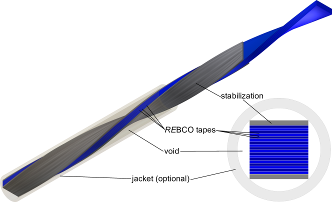
Figure 1: Schematic drawing of a Twisted Stacked-Tape Cable (TSTC). REBCO tapes are stacked and twisted. The mechanical and electrical stabilization is increased with copper tapes on the top and the bottom of the superconductor stack. To further improve the mechanical properties, the TSTC can be equipped with a jacket of structural material.

2 Sample parameters

A Twisted Stacked-Tape Cable sample of $1.16\text{\,}\mathrm{m}$ length consisting of 40, $4\text{\,}\mathrm{mm}$ wide copper stabilized SuperPower REBCO tapes with advanced pinning ($7.5\text{\,}\mathrm{a}\mathrm{t}\mathrm{\char 37\relax}$ Zr doping) is used in the following investigations. The tapes are arranged in one stack to which $0.25\text{\,}\mathrm{mm}$ thick copper tapes of the same width are attached to the top and the bottom for mechanical and thermal stabilization. The stack is twisted with a twist pitch of approximately $200\text{\,}\mathrm{mm}$ and is inserted into a copper tube of $7.9\text{\,}\mathrm{mm}$ outer diameter and $0.81\text{\,}\mathrm{mm}$ wall thickness. The hollow space between the stack and the tube is completely filled with soft solder preventing movement of the stack and dispersing mechanical loads. The sample contains two clamped BSCCO-REBCO connectors at its ends, which are described in detail in [14]. Four pairs of voltage taps are soldered onto the copper tube and one pair is attached to the copper terminations of the sample. All sample parameters are summarized in table 1.

Table 1: Parameters of the investigated Twisted Stacked-Tape Cable sample.

parameter	TSTC sample
sample length	$1.16\text{\,}\mathrm{m}$ including terminations
superconductor	$4\text{\,}\mathrm{mm}$ wide copper stabilized from SuperPower (SCS4050) - advanced pinning
number of tapes	40
twist pitch $\tau$	$200\text{\,}\mathrm{mm}$
termination	clamped BSCCO - REBCO  connections
mechanical stabilization	twisted stack soldered into Cu tube ($7.90\text{\,}\mathrm{mm}$ diameter, $0.81\text{\,}\mathrm{mm}$ wall thickness)
electrical stabilization	Cu stabilization of REBCO tapes + Cu tapes on top and bottom of the stack
voltage taps	4 pairs soldered onto the Cu tube, 1 pair at the Cu terminations

To determine the impact of transverse (radial direction) mechanical loads, magnetic background fields and temperature on the current carrying capabilities of Twisted Stacked-Tape Cables, the TSTC sample is characterized in three steps.

1. Impact of transverse mechanical loads by cycling the magnetic background fields and measuring the current carrying capabilities. Degradations due to the increasing Lorentz forces will be made visible in these measurements by comparing the obtained critical currents of different load cycles (subsection 4.1).

2. Critical current measurements at different fields and temperatures to determine the magnetic field and temperature dependence of Twisted Stacked-Tape Cables (subsection 4.2).

3. Critical current measurements at $77\text{\,}\mathrm{K}$, self-field after the in-field characterizations to determine the irreversible influence of the Lorentz forces onto the cable performance in different sections along the length of the sample (subsection 4.3).

3 Variable temperature insert

The experiments are performed using the FBI (force - field - current) superconductor test facility of the Institute for Technical Physics (ITEP) of the Karlsruhe Institute of Technology (KIT) [19]. The name “FBI” of the test facility is an abbreviation of the possible test parameters, F stands for force, B for magnetic field and I for current. It contains a superconducting split coil magnet, delivering magnetic background fields up to $12\text{\,}\mathrm{T}$, the field is orientated perpendicular to the sample axis with a homogeneous region ($97\text{\,}\mathrm{\char 37\relax}$ of peak field) of $70\text{\,}\mathrm{mm}$. A low noise direct current power supply delivers up to $10\text{\,}\mathrm{kA}$ to the sample. The test facility has been equipped with a variable temperature insert [20], as shown schematically in figure 2, to allow testing at sample temperatures above $4.2\text{\,}\mathrm{K}$. It consists of:

temperature sensors:

Two Cernox™temperature sensors [21] in direct contact with the sample to determine its surface temperature. Cernox sensors are used as this sensor type combines a high sensitivity at cryogenic temperatures with a very low magnetic field dependence.

heating foils:

Two Kapton^® heating foils of $100\text{\,}\mathrm{mm}$ length each wrapped around the sample. The heating power of the foils is controlled individually.

thermal insulation:

Double wall glass-fiber-reinforce-plastics (GFRP or G10) chamber of $400\text{\,}\mathrm{mm}$ length, containing gaseous helium during operation. The chamber fits tightly around the sample and is sealed at the upper and lower ends with adhesive tape and bees wax in order to minimizes the helium exchange.

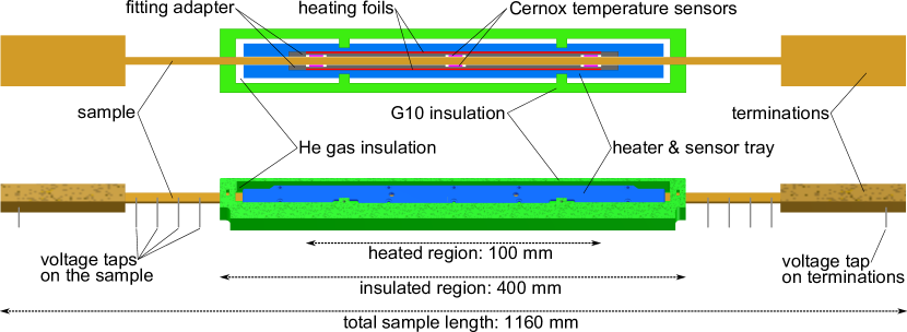
Figure 2: Variable temperature insert for the FBI test facility. The insert allows testing at sample temperatures from $4.277\text{\,}\mathrm{K}$. Schematic drawing in side view (upper), technical drawing (lower). Picture is not up to scale.

The measurement configuration used for the characterization of the Twisted Stacked-Tape Cable sample is shown schematically in figure 3.

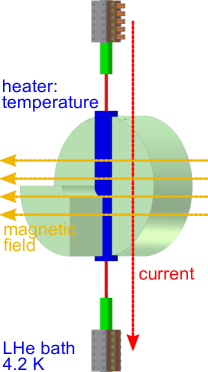
Figure 3: Schematic drawing of the superconductor test facility “FBI” with the variable temperature variable. The system allows critical current measurements on superconductor cables depending on magnetic background fields and temperatures.

3.1 Validation of the variable temperature insert

The performance of the variable temperature insert is validated on a CICC dummy consisting of a copper rod of $8\text{\,}\mathrm{mm}$ diameter inside a round stainless steel jacket with $1\text{\,}\mathrm{mm}$ of wall thickness. This assembly results in very low radial (transverse) and high longitudinal thermal conductivities and is therefore the worst case scenario for the variable temperature insert as heat is transferred radially from the heating foils to the sample and lost longitudinally to the helium bath. Four Cernox sensors are used to measure the temperature of the dummy at different positions. Two sensors (sensor positions 1 & 2) are located within the stainless steel jacket, just below the heating foils, reading the sample’s surface temperatures. The other two temperature sensors (sensor positions 3 & 4) are embedded in the dummy’s core. The layout of the dummy and the placement of the sensors is shown schematically in figure 4 (a). In figure 4 (b), the readout of these sensors is shown for different heating powers of the variable temperature insert.

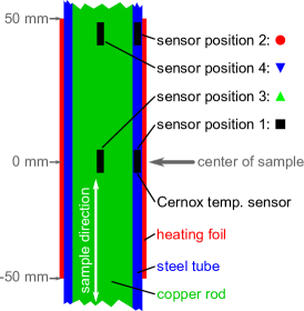
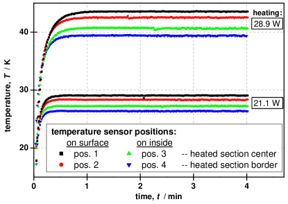
Figure 4: Validation of the variable temperature with a CICC dummy consisting of a copper rod inside a stainless steel tube representing a worst case scenario of HTS cables. Four Cernox temperature sensors are placed at different positions. Temperature sensor positions and the layout of the dummy are shown on in (a: left). The time dependent readout of the sensors is show for two different heating powers ($21.1\text{\,}\mathrm{W}$ and $28.9\text{\,}\mathrm{W}$) in (b: right).

These temperature sensors of the cable dummy are used to assess the performance of the variable temperature insert. Response time, stability and temperature distribution are analyzed.

3.1.1 Response time

The response of the variable temperature insert is fast in the investigated temperature range, due to all materials’ low heat capacities. It takes less than $1\text{\,}\mathrm{min}$ to heat up the sample and reach a stable temperature.

3.1.2 Stability

After the heating-up time, the measured temperatures are stable with flat temperature vs. time curves. Temperature variations at constant heating power remain below $0.3\text{\,}\mathrm{K}$ at all investigated temperatures and can be neglected. Thus, sample temperature are assumed to be constant after the heat up time.

3.1.3 Temperature distribution

A sample is surrounded with heating foils inside the variable temperature insert. Outside the insert, the sample remains immersed in the liquid helium bath. Heat is transported along the sample from the heated section to the helium bath. This heat flux depends on the temperature difference, the distance, the cross sectional area of the sample and the thermal conductivities of the constituent materials. Consequently the sample temperature is not homogenous; there is always a temperature gradient in the sample. The thermal conductivity of the jacket material is much lower compared with the conductivity of the central copper rod. Thus, the thermal conductivity of the cable is significantly higher in longitudinal direction than in transverse direction. Along the sample (longitudinal direction) the main part of the heat flux takes place in the copper center, resulting in a pronounced transverse temperature gradient. Due to the close proximity to the heating foils, the two temperature sensors on the surface of the sample (sensor positions 1 & 2) yield the highest temperatures. Inside the sample, the temperatures are significantly lower (sensor positions 3 &4 ). The precedence of the temperatures (pos. 1 > pos. 2 > pos. 3 > pos. 4) remains true for the investigated heating powers, just the differences between the sensors become increasingly pronounced with stronger heating. The main contribution reducing the temperature is therefore the transverse distance from the sample’s surface followed by the longitudinal distance from the center of the heated section. The temperature differences of the two sensors on the sample’s surface are less than $\pm 0.7\text{\,}\mathrm{K}$ event at the higher heating power. This low differences, justify the assumption that the sample’s surface temperature is homogeneous in all following investigations. Towards the inside of the sample, the temperature differences become more pronounced. The sample’s inside sensors register approximately $2\text{\,}\mathrm{K}$ lower temperatures than at the corresponding surface positions.

3.2 Temperature distribution of the Twisted Stacked-Tape Cable

There are two Cernox^® sensors are attached to the sample’s surface (one at the upper border of the heated section at position $-50\text{\,}\mathrm{mm}$ and the other in the center of the heated section at position at $0\text{\,}\mathrm{mm}$), however, in contrast to the cable dummy it is not possible to place temperature sensors inside the Twisted Stacked-Tape Cable sample. This precludes a fully experimental approach to determine the sample’s temperature distribution. Instead, the temperature distribution is calculated using Finite-Element-Method (FEM) models with the commercial software package “Comsol Multiphysics” [22] using the average of the two surface sensors as an input. In the following, this average is referred to as the sample’s surface temperature $T_{\textrm{surface}}$. Comparing with the HTS cable dummy’s experiments (subsection 3.1) it is clear that the temperature variations on the sample’s surface are not pronounced due to the close proximity to the heating foils, allowing the assumption of a homogenous surface temperature in the FEM model. The heated section of the sample is modeled at full scale (see table 1) in three dimensions using the direction and temperature dependent thermal conductivities of all constituent materials as shown in figure 5. The thermal conductivity of the REBCO tapes are mainly influenced in longitudinal direction by the copper stabilizer and in transverse direction by the Hastelloy^® substrate resulting in a three order of magnitude anisotropy [18, chap. 4.3.5].

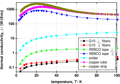
Figure 5: Thermal conductivity of the constituent materials of the investigated Twisted Stacked-Tape Cable sample in the operating temperature range of the variable temperature insert. Data from [23, 24, 18].

In the model, temperature sources (the heating foils: length $100\text{\,}\mathrm{mm}$) and temperature sinks (the helium bath outside the insulated area: length: $2\times$$150\text{\,}\mathrm{mm}$) are imposed as boundary conditions. For optimal resolution, different mesh configurations are used. The REBCO tapes are netted with a mapped mesh (mesh with explicit node locations) allowing the placement of several nodes within the width of each tapes’ superconducting layer. A free tetradic mesh, with much lower node density, is used in the variable temperature insert. This simulation method is shown schematically in figure 6.

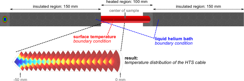
Figure 6: Schematic drawing of the FEM models used in the simulations of the temperature distribution of HTS cables in the variable temperature insert. An exemplary temperature distribution is shown as a color gradient from cold (blue) to hot (red). Drawing is not up to scale.

The temperature distribution is calculated for surface temperatures from $10100\text{\,}\mathrm{K}$. The temperatures of the nodes along the width of all tapes’ superconducting layers are averaged each $5\text{\,}\mathrm{mm}$ along length of the sample. These temperatures $T_{\textrm{average}}$ are shown in figure 7 from the border (position: $-50\text{\,}\mathrm{mm}$) to the center of the heating section (position: $0\text{\,}\mathrm{mm}$).

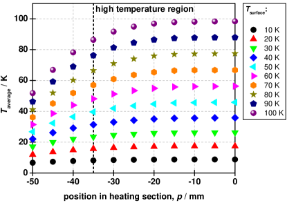
Figure 7: Simulated temperature distribution of a $40$-tape TSTC. The average temperature of the cable $T_{\textrm{average}}$ is shown at different positions in the heating section from the border (position: $-50\text{\,}\mathrm{mm}$) to the center (position: $0\text{\,}\mathrm{mm}$) of the $100\text{\,}\mathrm{mm}$ long heating section).

With the copper sheath and the copper tapes on the top and the bottom of the superconductor stack, the TSTC contains a lot of highly conductive material. They result in a significant thermal transport along the sample and leads to very low average temperatures near the borders of the heating section. A central $70\text{\,}\mathrm{mm}$ long region (from position $-35\text{\,}\mathrm{mm}$ to $35\text{\,}\mathrm{mm}$) with much lower temperature deviation, corresponding to the “high field region” of the test facility’s magnet is therefore defined as the “high temperature region” and the active zone of the variable temperature insert. Within this region, the temperature deviations are $20.2\text{\,}\mathrm{\char 37\relax}$ at $100\text{\,}\mathrm{K}$ surface temperature and $<14.4\text{\,}\mathrm{\char 37\relax}$ in the surface temperature range of interest for the experiments ($2040\text{\,}\mathrm{K}$). Outside this region, the temperature drops quickly. This means that in the temperature dependent characterization of the TSTC sample (subsection 4.2), $70\text{\,}\mathrm{mm}$ well defines the working area of the variable temperature insert. In this region the temperature varies no more than $\pm 2.7\text{\,}\mathrm{K}$, allowing REBCO ’s temperature dependence of the critical current to be assumed to be linear while averaging the temperature distribution. This zone, is therefore used to translate voltages into electric fields regardless of the separation of the voltage taps. Temperatures and magnetic fields are highest only inside this zone, limiting the whole sample’s current carrying capabilities. Outside of this zone, temperature and field are decreasing strongly. The contribution of the parts of the sample outside of the high field and high temperature region are determined by extrapolating the test facility’s magnetic field profile as well as the simulated temperature distribution. Using the field- and temperature dependence published by the tapes’ manufacturer, the current carrying capabilities are calculated depending on the position $p$ along the length of the sample for three scenarios: field active ($12\text{\,}\mathrm{T}$ magnetic background field), heating active ($40\text{\,}\mathrm{K}$ sample surface temperature) as well as field and heating active ($12\text{\,}\mathrm{T}$ magnetic background field at $40\text{\,}\mathrm{K}$ sample surface temperature). In order to make a worst case assumption, the resulting total voltages are obtained assuming a power-law behavior with a low n-value of $8$ (lowest n-value observed in all measurements of the TSTC sample, see figure 11). In figure 8, reciprocal normalized critical currents $I_{\textrm{c,max}}/I_{\textrm{c}}(p)$ and normalized total voltages $V_{\textrm{tot}}(p)/V_{\textrm{in}}$ are shown, the data is symmetric around the sample’s center, the zero position ($p=0$).

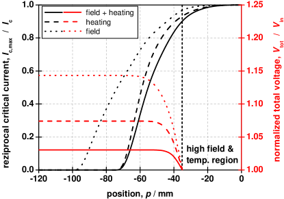
Figure 8: Extrapolated reciprocal normalized critical currents (in black) and normalized total voltages (in red) depending on the position along the sample for three scenarios: field active ($12\text{\,}\mathrm{T}$ magnetic background field), heating active ($40\text{\,}\mathrm{K}$ sample surface temperature) as well as field and heating active ($12\text{\,}\mathrm{T}$ magnetic background field at $40\text{\,}\mathrm{K}$ sample surface temperature).

The parts of the sample contribute $14\text{\,}\mathrm{\char 37\relax}$ if only the magnet is used, $7\text{\,}\mathrm{\char 37\relax}$ if solely the variable temperature insert is activated and $3\text{\,}\mathrm{\char 37\relax}$ in the case of magnetic background field and heating. These low contributions, especially in the case of magnetic background fields and heating, justify to neglect the parts of the sample outside the high field and high temperature zone. In these cases, voltages are only generated in the sample’s central $70\text{\,}\mathrm{mm}$ and this distance is used to convert the obtained voltages into electric fields.

4 Results

4.1 Critical current of magnetic field cycles

Initially, the cable is checked for degradation of the current carrying capabilities due to high transverse mechanical loads. This is achieved through cycling of the magnetic background field, currents and transverse loads. The magnetic background field is increased from zero field to $12\text{\,}\mathrm{T}$. Every $2\text{\,}\mathrm{T}$, the critical current is measured at $4.2\text{\,}\mathrm{K}$.

In the $812\text{\,}\mathrm{T}$ range, the current carrying capabilities of SuperPower advanced pinning REBCO tapes are only slightly reduced with magnetic field increases. Consequently, the Lorentz forces, and the transverse loads on the cable, are maximal at $12\text{\,}\mathrm{T}$. After reaching maximal field, and maximal transverse loads, the background field is reduced back to zero. Once again, the critical currents are measured every $2\text{\,}\mathrm{T}$. Any occurring degradation is exposed by comparing the critical currents measured at identical background fields on field increases and decreases. This procedure is repeated several times to detect further degradation of the sample. The measured critical currents are shown in figure 9. In these measurements, the sample is kept at $4.2\text{\,}\mathrm{K}$, the variable temperature insert is not activated. The voltage tap pair on the copper jacket with maximal separation (see figure 2) is used to average over the behavior of all the tapes. The sample includes two clamped BSCCO - REBCO connectors which are a very compact way of connecting the 40 REBCO tapes. However, as the contact resistances are not perfectly homogeneous, the sample’s tapes carry different fractions of the total current. These differences decrease with increasing voltage during the superconducting transition. A $5\text{\,}\mathrm{\SIUnitSymbolMicro V}\text{\,}{\mathrm{cm}}^{-1}$ criteria is therefore used to determine the critical currents in all in-field measurements of the TSTC sample. Furthermore, the inhomogeneous contact resistances and the following current redistribution result in a linear ohmic contribution during the critical current measurements. These are subtracted from the V-I curves before determining the critical currents. In this figure a field dependence of the critical currents calculated based on single tape data from [25] is shown between $6\text{\,}\mathrm{T}$ and $12\text{\,}\mathrm{T}$ by normalizing at $6\text{\,}\mathrm{T}$.

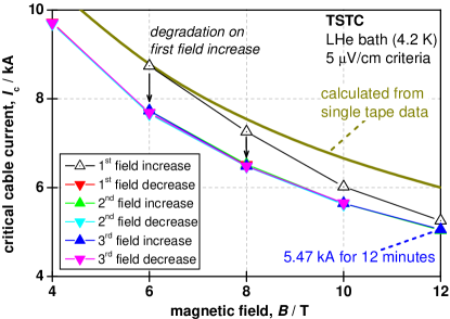
Figure 9: Critical current measurements at increasing and decreasing magnetic background fields of a $40$-tape TSTC. The voltage tap pair with maximal separation is used; linear ohmic contribution in the V-I curves is subtracted. Field dependence of the critical currents (yellow curve) is calculated based on single tape data from [25] and normalized at $6\text{\,}\mathrm{T}$.

On the first increase of the magnetic background field, the current carrying capabilities of the sample degrade. At $6\text{\,}\mathrm{T}$, the sample current is exactly as to be expected from the single tape tape. To higher magnetic background fields, the Twisted Stacked-Tape Cable sample carries lower current relative to the single tape data. The high Lorentz forces, step-by-step degrade the superconductor tapes with increasing fields. These degradations however do not continue during following magnetic field cycles. After the first cycle, the current carrying capabilities remain unchanged even if the TSTC is kept at the maximum current of $5.47\text{\,}\mathrm{kA}$ at $12\text{\,}\mathrm{T}$ for $12\text{\,}\mathrm{min}$. The critical currents measured on the first increase of the magnetic field and on later field cycles are shown in table 2. The current carrying capabilities of all magnetic field cycles but the first field increase are averaged.

Table 2: Degradation of a $40$-tape Twisted Stacked-Tape Cable due to transverse mechanical loads at high magnetic background fields. Critical currents of field cycles, following on the first magnetic field increase, are averaged.

field	critical current - first increase	critical current - later	degradation
$6\text{\,}\mathrm{T}$	$8.74\text{\,}\mathrm{kA}$	$7.70\text{\,}\mathrm{kA}$	$11.9\text{\,}\mathrm{\char 37\relax}$
$8\text{\,}\mathrm{T}$	$7.26\text{\,}\mathrm{kA}$	$6.50\text{\,}\mathrm{kA}$	$10.5\text{\,}\mathrm{\char 37\relax}$
$10\text{\,}\mathrm{T}$	$6.02\text{\,}\mathrm{kA}$	$5.64\text{\,}\mathrm{kA}$	$6.3\text{\,}\mathrm{\char 37\relax}$
$12\text{\,}\mathrm{T}$	$5.26\text{\,}\mathrm{kA}$	$5.05\text{\,}\mathrm{kA}$	$4.0\text{\,}\mathrm{\char 37\relax}$

Determination of degradation is not possible at fields of $4\text{\,}\mathrm{T}$ and below as the critical currents of the sample are above the maximal current of the test facility ($10\text{\,}\mathrm{kA}$). At background fields of $6\text{\,}\mathrm{T}$, a maximal degradation of $11.9\text{\,}\mathrm{\char 37\relax}$ is obtained. For higher fields, the degradation decreases. The non-constant degradation implies that damage to the sample occurs not just during the critical current measurement at maximal field. Some degradation already occurs below maximal magnetic fields. The factor of degradation is close at $6\text{\,}\mathrm{T}$ and $8\text{\,}\mathrm{T}$, signifying that the biggest fraction of the total degradation is occurring at higher magnetic background fields.

Transverse mechanical loads can degrade the REBCO tapes in TSTCs, these degradations are described above. In the investigated sample, the hollow space between the stack of superconductor tapes and the copper jacket is quite well filled with soft solder by liquifying and injecting the solder through holes in the jacket while the sample is heated on a heating plate. However, the solder did not support well the Lorentz forces, allowing a movement of the stack leading to a degradation of the superconductor tapes. Due to the superior mechanical properties and to possibility to be drawn into the sample with vacuum would make low thermal expansion epoxy resin mixtures superior filling agents which may have prevented such sample degradations [26].

4.2 Temperature dependence at different background fields

In this part of the TSTC sample characterization, the variable temperature insert of the FBI test facility is utilized. The critical currents are measured in each of the $2\text{\,}\mathrm{T}$ magnetic background field steps for different cable surface temperatures. It was attempted to obtain the same sample surface temperature steps in the whole magnetic field range. The two copper tapes on the top and the bottom of the REBCO tapes stack, the solder and the encasing copper tube electrically stabilize the sample. The stabilization is sufficient, no thermal runaway is observed, even during superconducting transitions close to$10\text{\,}\mathrm{kA}$ transport current. Within the heated section, two temperature sensors are attached to the sample’s surface (one at the upper border of the heated section at position $-50\text{\,}\mathrm{mm}$ and the other in the center of the heated section at position at $0\text{\,}\mathrm{mm}$). As expected from the validation of the variable temperature insert (subsection 3.1), their readouts are very similar (within $\pm 0.9\text{\,}\mathrm{K}$ in the investigated range of heating powers) and their average value is therefore referred to as the samples surface temperature $T_{\textrm{surface}}$. In figure 10, the current carrying capabilities of the TSTC sample are shown for sample surface temperatures from $4.2\text{\,}\mathrm{K}$ to $37.8\text{\,}\mathrm{K}$ using a $5\text{\,}\mathrm{\SIUnitSymbolMicro V}\text{\,}{\mathrm{cm}}^{-1}$ criteria assuming an active region of the magnetic field and the temperature of $70\text{\,}\mathrm{mm}$. Linear ohmic contribution in the V-I curves is subtracted. From the experimental point of view it has to be noted that the twist pitch of the sample is with $200\text{\,}\mathrm{mm}$ (see table 1) larger than the $70\text{\,}\mathrm{mm}$ long high field and high temperature region. The tapes are therefore not exposed to all orientations of the magnetic background field adding some uncertainty to the gained field dependence due to REBCO’s anisotropy.

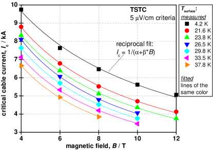
Figure 10: Field and surface temperature dependent measurements of a 40-tape TSTC. The measurements (points) use the voltage taps on the copper jacket with maximal separation. Linear ohmic contribution in the V-I curves is subtracted. Critical currents are determined with the $5\text{\,}\mathrm{\SIUnitSymbolMicro V}\text{\,}{\mathrm{cm}}^{-1}$ criteria assuming a active region of $70\text{\,}\mathrm{mm}$ for field and temperatures. Data is fitted with reciprocal functions (lines).

The curves of different surface temperatures are regularly spaced and are of reciprocal shape ($I_{\textrm{c}}=\frac{1}{\left(\alpha+\beta\cdot B\right)}$). The n-values are calculated for all superconducting transitions of the field and temperature dependent measurements. The calculations are done in the electric field range from $1\text{\,}\mathrm{\SIUnitSymbolMicro V}\text{\,}{\mathrm{cm}}^{-1}$ to $10\text{\,}\mathrm{\SIUnitSymbolMicro V}\text{\,}{\mathrm{cm}}^{-1}$. The same voltage taps are used, assuming an active region of field and temperature of $70\text{\,}\mathrm{mm}$. The n-values are shown in figure 11.

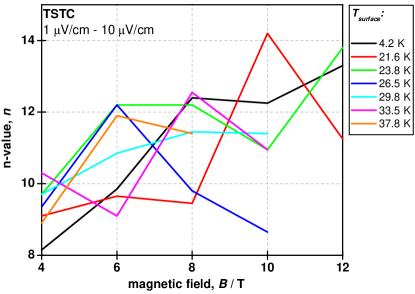
Figure 11: The n-values of the superconducting transitions of a $40$ tape TSTC. The measurements are of the degraded cable at different cable temperatures and magnetic background fields. The n-values are calculated in the electric field range $110\text{\,}\mathrm{\SIUnitSymbolMicro V}\text{\,}{\mathrm{cm}}^{-1}$ using the voltage tap pair on the copper jacket with maximal separation. Linear ohmic contribution in the V-I curves is subtracted.

As could be expected from the sample layout, all n-values are low, they are in the $8$ to $14$ range. There are two aspects contributing to the low n-values. Firstly, the inhomogeneous contact resistances of the two REBCO - BSCCO connectors, and the resulting current redistribution. The tapes do not carry the same fraction of the total current and therefore begin their transition from superconducting state to normal conduction at different cable currents. As the voltage is read at the copper sheath it corresponds to an averaging of the behavior of all tapes. This “smears” the transition and lowers the n-values.Secondly, the degradation of the sample, which occurred on the first field increase. Some of the REBCO tapes were damaged, reducing the current they can carry. This damage strongly in-homogenizes the sample, causing the tapes to generate voltages at very low cable currents. In a non-degraded TSTC, significantly higher n-values are therefore to be expected.

Using the temperature distribution obtained in the FEM model of the TSTC sample (subsection 3.2), average sample temperatures $T_{\textrm{avg}}$ are calculated for the measured surface temperatures $T_{\textrm{surface}}$ by averaging the distribution in the $70\text{\,}\mathrm{mm}$ long high temperature region. These temperatures as well as the statistic (from the averaging and the FEM model) and the systematic (from the temperature measurement) temperature uncertainty are shown in table 3.

Table 3: Sample surface temperatures $T_{\textrm{surface}}$, average sample temperatures $T_{\textrm{avg}}$, statistic and systematic measurement uncertainty derived from the FEM model of the TSTC sample.

surface temperature, $T_{\textrm{surface}}$	average temperature, $T_{\textrm{average}}$	statistic uncertainty	systematic uncertainty
$4.2\text{\,}\mathrm{K}$	$4.2\text{\,}\mathrm{K}$	-	-
$21.6\text{\,}\mathrm{K}$	$18.3\text{\,}\mathrm{K}$	$\pm 0.6\text{\,}\mathrm{K}$	$\pm 0.3\text{\,}\mathrm{K}$
$23.8\text{\,}\mathrm{K}$	$20.2\text{\,}\mathrm{K}$	$\pm 0.9\text{\,}\mathrm{K}$	$\pm 0.4\text{\,}\mathrm{K}$
$26.5\text{\,}\mathrm{K}$	$22.5\text{\,}\mathrm{K}$	$\pm 1.0\text{\,}\mathrm{K}$	$\pm 0.4\text{\,}\mathrm{K}$
$29.8\text{\,}\mathrm{K}$	$25.4\text{\,}\mathrm{K}$	$\pm 1.1\text{\,}\mathrm{K}$	$\pm 0.6\text{\,}\mathrm{K}$
$33.5\text{\,}\mathrm{K}$	$28.9\text{\,}\mathrm{K}$	$\pm 1.3\text{\,}\mathrm{K}$	$\pm 0.7\text{\,}\mathrm{K}$
$37.8\text{\,}\mathrm{K}$	$32.7\text{\,}\mathrm{K}$	$\pm 1.6\text{\,}\mathrm{K}$	$\pm 0.9\text{\,}\mathrm{K}$

4.3 Characterization at $77\text{\,}\mathrm{K}$, self-field after the in-field measurements

Following the described magnetic field and temperature tests at the FBI facility, the tested sample was sent back to MIT, and the critical currents were tested at $77\text{\,}\mathrm{K}$ in a liquid nitrogen bath without a magnetic background field (self-field conditions) [15]. Two regions of the conductor were tested: one at the center section which was tested in the high field at the FBI and the other near the end of the conductor which was not exposed to the high field. The critical current test results were $1.70\text{\,}\mathrm{kA}$ at the $1\text{\,}\mathrm{\SIUnitSymbolMicro V}\text{\,}{\mathrm{cm}}^{-1}$ criterion with an n-value of $12$ for the center region and $1.99\text{\,}\mathrm{kA}$ with an n-value of $26$ at the end region. It indicates the center region had degraded by $15\text{\,}\mathrm{\char 37\relax}$ during the high field test at the FBI test facility, the n-value of the center region is in very good agreement with with the n-value range observed during the field- and temperature dependent measurements. It is also noted that the linear ohmic contribution in the V-I curve was as small as $2.1\text{\times}{10}^{-9}\text{\,}\mathrm{\SIUnitSymbolOhm}$, less than that observed at the high field experiments at the FBI test. A larger linear ohmic component during the FBI tests is to be expected as the active region of fields and temperatures is with $70\text{\,}\mathrm{mm}$ rather small. Thus, the voltage during the superconducting transitions are low, making the current redistribution due to the contact resistance inhomogeneities more pronounced. Transverse load test performed after the critical current tests at $77\text{\,}\mathrm{K}$ was shown additional degradation by only $3\text{\,}\mathrm{\char 37\relax}$ for the center region, on the other hand by $20\text{\,}\mathrm{\char 37\relax}$ for the end region by the external transverse load of $400\text{\,}\mathrm{kN}\text{\,}{\mathrm{m}}^{-1}$. Further transverse load test results can be obtained in [15].

5 Discussion and conclusion

The performance of the variable temperature insert of the FBI test facility has been evaluated with a CICC dummy. Temperature sensors on the surface and the inside of the dummy are used to determine, the response time, the stability and the temperature distribution of the dummy. In the temperature range of interest in less than one minute, the temperatures are stable, however there is a strong temperature gradient from the surface to the inside of the sample. The temperature readouts of the sensors on the surface are similar, allowing the use their average in the following. As it is not possible to place sensors on the inside of the TSTC sample, it is modeled in 3D in full scale using the temperature and direction dependent properties of its constituent materials. From this FEM model the working area of the variable temperature insert is determined to be $70\text{\,}\mathrm{mm}$ with a temperature variation of less than $14.4\text{\,}\mathrm{\char 37\relax}$. In the utilized temperature range this corresponds to deviations of less than $\pm 2.7\text{\,}\mathrm{K}$ from the average temperature. Averaging assumes a linear temperature dependence of the critical current for the REBCO tapes, which is acceptable in such small temperature range, far below the critical temperature. Outside this high temperature zone the sample temperature drops quickly. The zone corresponds to the high field region of the magnet, therefore this $70\text{\,}\mathrm{mm}$ are used to transform voltages into electric fields in all FBI measurements of the TSTC sample regardless of the separation of the voltage taps. The current carrying capabilities of the the 40-tape Twisted Stacked Tape Cable sample are tested at various magnetic background fields of up to $12\text{\,}\mathrm{T}$. At higher magnetic fields, the enormous Lorentz forces of up to $65.6\text{\,}\mathrm{kN}\text{\,}{\mathrm{m}}^{-1}$ result in an irreversible degradation of the sample’s transport current. In the following field cycles, the degradation does not continue, it saturates at $11.8\text{\,}\mathrm{\char 37\relax}$. Using the variable temperature insert, the current carrying capabilities of the sample are measured in up to $12\text{\,}\mathrm{T}$ magnetic background fields and sample surface temperatures of up to $37.8\text{\,}\mathrm{K}$. Using the temperature distribution obtained in the FEM model, the average sample temperature and the temperature uncertainty is calculated. Critical current index n-values in the range of $8-14$ are obtained during these measurements. Two separate aspects are likely contributing to the low n-values: Firstly, and secondly the inhomogeneous contact resistances of the sample’s clamped REBCO - BSCCO connectors which cause the tapes to carry different fractions of the total current and to start their superconducting transitions at different cable currents.. Secondly, the sample’s degradation, meaning damage to some of the REBCO tapes resulting in strong current redistribution already at low cable currents. Higher n-values are to be expected in non-degraded TSTCs. As the active zone of the fields and temperatures ($70\text{\,}\mathrm{mm}$) is lower the TSTC sample’s twist pitch ($200\text{\,}\mathrm{mm}$), we cannot compare the cable’s performance with the field- and temperature dependence of single tapes’ critical currents. Following on the magnetic field and temperature tests at the FBI facility, the tested sample is characterized at $77\text{\,}\mathrm{K}$, self-field. The center region of the cable, which was exposed to the high transverse Lorentz forces during the in-field measurements, the current carrying capabilities are reduced by $15\text{\,}\mathrm{\char 37\relax}$. This corresponds well to the behavior observed during the magnetic field cycles.

References

- [1] W Goldacker, R Nast, G Kotzyba, S I Schlachter, a Frank, B Ringsdorf, C Schmidt, and P Komarek. High current DyBCO-ROEBEL Assembled Coated Conductor (RACC). Journal of Physics: Conference Series, 43:901–904, June 2006.
- [2] N J Long, R A Badcock, K Hamilton, A Wright, Z Jiang, and L S Lakshmi. Development of YBCO Roebel cables for high current transport and low AC loss applications. Journal of Physics: Conference Series, 234:022021, 2010.
- [3] N J Long. HTS Roebel cables. In HTS4Fusion Conductor Workshop, KIT CN, Karlsruhe, 2011.
- [4] N J Long, R A Badcock, C W Bumby, Z Jiang, and R G Buckley. Production and characterisation of HTS roebel cable. In M Miryala, editor, Superconductivity: Recent Developments and New Production Technologies, chapter 13, pages 259–288. Nova Science Publishers, Inc., Huntington, 2012.
- [5] S I Schlachter, W Goldacker, F Grilli, R Heller, and A Kudymow. Coated Conductor Rutherford Cables (CCRC) for High-Current Applications: Concept and Properties. IEEE Transactions on Applied Superconductivity, 21(3):3021–3024, June 2011.
- [6] A Kario, M Vojenciak, F Grilli, A Kling, B Ringsdorf, U Walschburger, S I Schlachter, and W Goldacker. Investigation of a Rutherford cable using coated conductor Roebel cables as strands. Superconductor Science and Technology, 26(8):085019, August 2013.
- [7] D C van der Laan. YBa2Cu3O7-delta coated conductor cabling for low ac-loss and high-field magnet applications. Superconductor Science and Technology, 22(6):065013, June 2009.
- [8] D C van der Laan, X F Lu, and L F Goodrich. Compact GdBa2Cu3O7- coated conductor cables for electric power transmission and magnet applications. Superconductor Science and Technology, 24(4):042001, April 2011.
- [9] D C van der Laan, L F Goodrich, and T J Haugan. High-current dc power transmission in flexible RE-Ba2Cu3O7- coated conductor cables. Superconductor Science and Technology, 25(1):014003, January 2012.
- [10] D C van der Laan, P D Noyes, G E Miller, H W Weijers, and G P Willering. Characterization of a high-temperature superconducting conductor on round core cables in magnetic fields up to 20 T. Superconductor Science and Technology, 26(4):045005, April 2013.
- [11] M Takayasu, J V Minervini, and L Bromberg. US patent: Superconductor Cable (patent number: 8 437 819 B2), 2009.
- [12] M Takayasu, L Chiesa, L Bromberg, and J V Minervini. Cabling Method for High Current Conductors Made of HTS Tapes. Applied Superconductivity, IEEE Transactions on, 21(3):2340–2344, 2011.
- [13] M Takayasu, J V Minervini, L Bromberg, M K Rudziak, and T Wong. Investigation of Twisted Stacked-Tape Cable Conductor. AIP Conference Proceedings, 1435:273–280, 2012.
- [14] M Takayasu, L Chiesa, L Bromberg, and J V Minervini. HTS twisted stacked-tape cable conductor. Superconductor Science and Technology, 25(1):014011, January 2012.
- [15] L Chiesa, N C Allen, and M Takayasu. Electromechanical Investigation of 2G HTS Twisted Stacked-Tape Cable Conductors. IEEE Transactions on Applied Superconductivity, 24(3):6600405, June 2014.
- [16] G Celentano, G De Marzi, F Fabbri, L Muzzi, G Tomassetti, A Anemona, S Chiarelli, M Seri, A Bragagni, and A della Corte. Design of an Industrially Feasible Twisted-Stack HTS Cable-in-Conduit Conductor for Fusion Application. IEEE Transactions on Applied Superconductivity, 24(3):4601805, 2014.
- [17] D Uglietti, R Wesche, and P Bruzzone. Fabrication Trials of Round Strands Composed of Coated Conductor Tapes. IEEE Transactions on Applied Superconductivity, 23(3):4802104, 2013.
- [18] C Barth. High Temperature Superconductor Cable Concepts for Fusion Magnets. KIT Scientific Publishing, Karlsruhe, 1. edition, 2013.
- [19] C M Bayer, C Barth, P V Gade, K Weiss, and R Heller. FBI Measurement Facility for High Temperature Superconducting Cable Designs. IEEE Transactions on Applied Superconductivity, 24(3):9500604, 2014.
- [20] C Barth, K-P Weiss, W Goldacker, and S I Schlachter. Electro-magnetic measurements of coated conductor cables at different temperatures. In MEM11 Workshop, Okinawa, 2011.
- [21] Lakeshore® Cryotronics Inc. Cernox™ temperature sensor.
- [22] COMSOL Inc. COMSOL Multiphysicstextsuperscript®.
- [23] N Bagrets, C Barth, and K Weiss. Low Temperature Thermal and Thermo-Mechanical Properties of Soft Solders for Superconducting Applications. IEEE Transactions on Applied Superconductivity, 24(3):7800203, 2014.
- [24] N Bagrets, W Goldacker, S I Schlachter, and C Barth. Thermal properties of 2G coated conductor cable materials. CRYOGENICS, 61:8–14, 2014.
- [25] D W Hazelton. 2G HTS Conductors at SuperPower. In Low Temperature High Field Superconductor Workshop, Napa, 2012. SuperPower.
- [26] C Barth, N Bagrets, K-P Weiss, C M Bayer, and T Bast. Degradation free epoxy impregnation of REBCO coils and cables. Superconductor Science and Technology, 26(5):055007, 2013.