A robust inversion method for quantitative 3D shape reconstruction from coaxial eddy-current measurements

Abstract

This work is motivated by the monitoring of conductive clogging deposits in steam generator at the level of support plates. One would like to use monoaxial coils measurements to obtain estimates on the clogging volume. We propose a 3D shape optimization technique based on simplified parametrization of the geometry adapted to the measurement nature and resolution. The direct problem is modeled by the eddy current approximation of time-harmonic Maxwell’s equations in the low frequency regime. A potential formulation is adopted in order to easily handle the complex topology of the industrial problem setting. We first characterize the shape derivatives of the deposit impedance signal using an adjoint field technique. For the inversion procedure, the direct and adjoint problems have to be solved for each coil vertical position which is excessively time and memory consuming. To overcome this difficulty, we propose and discuss a steepest descent method based on a fixed and invariant triangulation. Numerical experiments are presented to illustrate the convergence and the efficiency of the method.

siscxxxxxxxx–x

1 Introduction

Non-destructive testing using eddy-current low frequency excitation are widely practiced to detect magnetite deposits in steam generators (SG) in nuclear power plants. These deposits, due to magnetite particles contained in the cooling water, usually accumulate around the quatrefoil support plates (SP) and thus clog the water traffic lane. Many methods and softwares based on signal processing has been developed in order to detect deposits using standard bobbin coils and are widely operational in the nuclear industries (see for instance the database of nondestructive testing [10] and references therein). Estimates of the bulk amount of deposits enable to supplement a chemical cleaning process, which in some cases may be ineffective where it leaves significant deposits in the bottom area of the SP foils. The presence of such deposits generates a reduction and re-distribution of the water in SG circulation and can cause flow-induced vibration instability risks. This may harm the safety of the nuclear power plant.

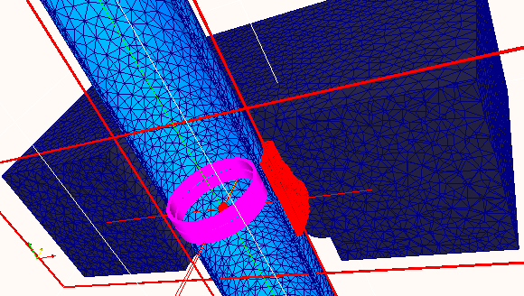
Fig. 1: Three dimensional mesh of the SG and the SP clogging : coils (pink), tube (blue), SP (grey) and deposit (red).

In order to obtain better characterizations than those provided by model free methods, we present and discuss a robust inversion algorithm (for non destructive evaluation using eddy current signals) based on shape optimization techniques and adapted parametrizations for the deposit shapes. An overview of techniques for non destructive evaluations using eddy currents can be found in [7] and we also refer to [23], [20] and [26] for further engineering considerations. For other model based inversion methods related to eddy-currents we may refer, without being exhaustive, to [8, 17, 16, 25, 6]. In the medical context, several inverse source problems related to eddy-current models have been addressed: non-invasive applications for electroencephalography, magnetoencephalography[3] (see also [1]) and magnetic induction tomography [12, 21].

Stated more precisely, the inverse shape problem we shall investigate aims at retrieving the support of a conductive deposits using monostatic measurements of coaxial coils and their computable shape derivatives. Our work can be seen as an extension of [18] to a realistic 3D industrial configuration. Although the deposit geometry can be an arbitrary three dimensional domain, the available (monostatic) measurements can only give qualitative information on the width. Since the objective is to detect the possibility of clogging at the support plate, we found it appropriate to consider a deposit concentrated in only one of the opening regions at the support plate (See Figs. 1). The geometrical parameters are then the deposit width at (at most) one measurement position. In practice, it turned out that a relative robustness with respect to noise can be achieved if one shape parameter correspond with two vertical positions of the coils. In order to speed up the inversion procedure, we are led to consider a fixed geometrical mesh (adapted to the chosen parametrization). This allows us to obtain an inversion procedure which is not very sensitive to the number of measurements. Moreover, in order to avoid troubles due to changes in the conductive region topology, we adopted a vector potential formulation of the 3D eddy-current model. A careful study of the shape derivative of the solution to this formulation is conducted. For related shape derivatives associated with Maxwell’s equations we refer to [9, 15]. We here treat the potential formulation of the eddy current problem. This derivative allows us to rigorously define the adjoint state, needed to cheaply compute the coils impedances shape derivatives.

The geometrical setting of the industrial configuration is depicted in Fig. 1. We denote by $\Omega$ the computational domain, which will be a sufficiently large simply connected cylinder. It contains a conductor domain $\Omega_{\mathcal{C}}$ composed of the tube, the support plate and eventually a deposit on the exterior part of the tube: $\Omega_{\mathcal{C}}=\Omega_{t}\cup\Omega_{d}\cup\Omega_{p}$, where $t$ stands for the tube, $d$ for the deposit and $p$ for the SP. The insulator domain $\Omega\setminus\overline{\Omega}_{\mathcal{C}}$ is split into two parts: $\Omega_{s}$ that indicates the region inside the tube where the coil (thus the source J) is located and $\Omega_{v}$ that denotes the insulator outer region (where the deposit can be formed). For our purpose we introduce the surface $\Gamma=\overline{\partial\Omega_{d}}\cap\overline{\partial\Omega_{v}}$ that denotes the interface between the deposit and the insulator.

Let us now briefly describe the 3D eddy-current model, which derives from the full Maxwell’s equation in the time harmonic low frequency case and the adopted formulation of this problem. Given the bounded domain $\Omega\subset\mathbb{R}^{3}$, we recall the time-harmonic Maxwell equations:

$$\begin{array}[]{lllr}&\operatorname{curl}\textbf{H}+(\mathrm{i}\omega\epsilon-\sigma)\textbf{E}&=\textbf{J}&\text{ in }\Omega,\\ &\operatorname{curl}\textbf{E}-\mathrm{i}\omega\mu\textbf{H}&=0&\text{ in }\Omega,\end{array}$$

and on the boundary $\partial\Omega$ we impose a magnetic boundary condition $\textbf{H}\times\bm{n}=0$, where $\bm{n}$ stands for the outward normal to the boundary $\partial\Omega$. Here H and E denotes the magnetic and electric fields, respectively. J is the applied current density, $\epsilon$ is the electric permittivity, $\mu$ is the magnetic permeability and $\sigma$ is the electric conductivity. In our case, the applied current density has support strictly included in the insulator $\Omega_{t}$(interior of the tube). By neglecting the displacement current term, we formally obtain the eddy-current model, which reads:

(1) $$\begin{array}[]{lllr}&\operatorname{curl}\textbf{H}&=\sigma\textbf{E}+\textbf{J}&\text{ in }\Omega,\\ &\mu\textbf{H}&=\dfrac{1}{\mathrm{i}\omega}\operatorname{curl}\textbf{E}&\text{ in }\Omega,\end{array}$$

We refer to the monograph [2] for an extensive overview of eddy-current models and formulations. In this paper we adopt a potential formulation in which we look for the magnetic vector potential A and electric scalar potential $V$ (only defined on $\Omega_{\mathcal{C}}$) that satisfies

(2) $$\left\{\begin{array}[]{rll}\mu\textbf{H}&=\operatorname{curl}\textbf{A}&\text{ in }\Omega,\\ \operatorname{curl}\textbf{H}&=\sigma\textbf{E}+\textbf{J}&\text{ in }\Omega,\\ \textbf{E}&=\mathrm{i}\omega\textbf{A}+\nabla V&\text{ in }\Omega_{\mathcal{C}},\\ \mathrm{div}\,\textbf{A}&=0&\text{ in }\Omega.\\ \bm{n}\times\dfrac{1}{\mu}\operatorname{curl}\textbf{A}&=0&\text{ on }\partial\Omega,\\ \textbf{A}\cdot\bm{n}&=0&\text{ on }\partial\Omega,\end{array}\right.$$

where the equation (2)₄ stands for the Coulomb gauge condition. The boundary condition (2)₅ stands for the magnetic boundary condition and the boundary condition (2)₆ is equivalent to $\epsilon\textbf{E}\cdot\bm{n}=0$. The electric scalar potential $V$ is determined up to an additive constant in each connected-component of $\Omega_{\mathcal{C}}$, which has a connected boundary.

Notice that from Maxwell-Ampère equation (1)₁ we get

(3) $$\operatorname{curl}(\mu^{-1}\operatorname{curl}\textbf{A})-\sigma(\mathrm{i}\omega\textbf{A}+\nabla V)=\textbf{J}\mbox{ in }\Omega.$$

In the following, the space $H(\operatorname{curl};\Omega)$ indicates the set of real or complex valued functions ${\bf v}\in(L^{2}(\Omega))^{3}$ such that $\operatorname{curl}{\bf v}\in(L^{2}(\Omega))^{3}$ and define

$$\mathcal{X}(\Omega):=\{{\bf v}\in H(\operatorname{curl},\Omega),\mathrm{div}\,{\bf v}=0\text{ in }\Omega,{\bf v}\cdot\bm{n}=0\text{ on }\partial\Omega\}.$$

For a vector magnetic potential $\textbf{A}\in\mathcal{X}(\Omega)$, an electric scalar potential $V\in H^{1}\left(\Omega_{\mathcal{C}}\right)/\mathbb{C}$ (the quotient by constants is relative to each connected component separately) and a test function $\bm{\Psi}\in\mathcal{X}(\Omega)$ the weak formulation of (3) reads

(4) $$\int_{\Omega}\dfrac{1}{\mu}\operatorname{curl}\textbf{A}\cdot\operatorname{curl}\overline{\bm{\Psi}}\thinspace\mathrm{d}x-\int_{\Omega_{\mathcal{C}}}\sigma\left(\mathrm{i}\omega\textbf{A}\cdot\overline{\bm{\Psi}}+\nabla V\cdot\overline{\bm{\Psi}}\right)\thinspace\mathrm{d}x=\int_{\Omega}\textbf{J}\cdot\overline{\bm{\Psi}}.$$

Moreover, for any test function $\varPhi\in H^{1}\left(\Omega_{\mathcal{C}}\right)/\mathbb{C}$ the weak formulation of the necessary condition $-\mathrm{div}\,\left(\sigma\textbf{E}\right)=\mathrm{div}\,\textbf{J}$ writes $-\int_{\Omega_{\mathcal{C}}}\sigma\textbf{E}\cdot\nabla\overline{\varPhi}\thinspace\mathrm{d}s=\int_{\Omega_{\mathcal{C}}}\textbf{J}\cdot\nabla\overline{\varPhi}\thinspace\mathrm{d}s$. Therefore using (2)₃ we obtain:

(5) $$-\sigma\int_{\Omega_{\mathcal{C}}}\left(\mathrm{i}\omega\textbf{A}+\nabla V\right)\cdot\nabla\overline{\varPhi}\thinspace\mathrm{d}x=\int_{\Omega_{\mathcal{C}}}\textbf{J}\cdot\nabla\overline{\varPhi}\thinspace\mathrm{d}x.$$

Following [2, Chp-6] (and references therein), by introducing a constant $\mu_{*}$, representing a suitable average of $\mu$ in $\Omega$, the Coulomb gauge condition (2)₃ can be incorporated in equation (4) in the following way

(6) $$\int_{\Omega}\dfrac{1}{\mu}\operatorname{curl}\textbf{A}\cdot\operatorname{curl}\overline{\bm{\Psi}}\thinspace\mathrm{d}x+\dfrac{1}{\mu_{*}}\int_{\Omega}\mathrm{div}\,\textbf{A}\mathrm{div}\,\overline{\bm{\Psi}}\thinspace\mathrm{d}x-\int_{\Omega_{\mathcal{C}}}\sigma\left(\mathrm{i}\omega\textbf{A}\cdot\overline{\bm{\Psi}}+\nabla V\cdot\overline{\bm{\Psi}}\right)\thinspace\mathrm{d}x=\int_{\Omega}\textbf{J}\cdot\overline{\bm{\Psi}}.$$

and the variational space $\mathcal{X}(\Omega)$ would then be replaced by $\mathcal{H}(\Omega):=H(\operatorname{curl},\Omega)\cap H_{0}(\mathrm{div}\,,\Omega)$ or equivalently by $H^{1}(\Omega)^{3}$ since the domain $\Omega$ is convex and sufficiently regular. Indeed, $\mathrm{div}\,\textbf{A}=0$ is verified in the weak sense. Combining equations (6) with (5) we can obtain a symmetric variational formulation as follows

(7) $$\mathcal{S}(\textbf{A},V;\bm{\Psi},\Phi)=\int_{\Omega}\textbf{J}\cdot\overline{\bm{\Psi}}\thinspace\mathrm{d}x-\dfrac{1}{\mathrm{i}\omega}\int_{\Omega_{\mathcal{C}}}\textbf{J}\cdot\nabla\overline{\Phi}\thinspace\mathrm{d}x\qquad\forall\,(\bm{\Psi},\Phi)\in\mathcal{Q},$$

where the sesquilinear form $\mathcal{S}$ is defined by:

(8) $$\begin{array}[]{lll}\mathcal{S}(\textbf{A},V;\bm{\Psi},\Phi)&:=&\displaystyle\int_{\Omega}\left(\dfrac{1}{\mu}\operatorname{curl}\textbf{A}\cdot\operatorname{curl}\overline{\bm{\Psi}}+\dfrac{1}{\mu_{*}}\mathrm{div}\,\textbf{A}\mathrm{div}\,\overline{\bm{\Psi}}\right)\thinspace\mathrm{d}x\\ &&+\displaystyle\dfrac{1}{\mathrm{i}\omega}\int_{\Omega_{\mathcal{C}}}\sigma(\mathrm{i}\omega\textbf{A}+\nabla V)\cdot(\overline{\mathrm{i}\omega\bm{\Psi}+\nabla\Phi})\thinspace\mathrm{d}x.\end{array}$$

The coercivity of $\mathcal{S}$ on $H^{1}(\Omega)^{3}\times H^{1}\left(\Omega_{\mathcal{C}}\right)/\mathbb{C}$ (see for instance [2, Chp-6]) ensures the well-posedness of the problem.

This paper is organized as follows: after this introduction, we state in Section 2 the nonlinear shape optimization problem by the introduction of the misfit function, which depends on the shape of the defect and in particular its eddy-current signal response. We derive, in Section 3, the adjoint problem which is based on the shape derivative of the misfit function. At the end of this Section we explicitly formulate the shape gradient via the adjoint problem. In Section 4, we present and explain the algorithm of steepest descent based on the use of fixed predefined grid. With Section 5, we conclude the paper with numerical experiments that illustrate the robustness of the method. Some technical materials related to shape derivative are reported in the appendix for the readers’ convenience.

We conclude this section with the introduction of some useful notations. We denote by $[\cdot]$ the jump across the interface $\Gamma$: $\left[F\right]=\lim_{t\searrow 0}F(x+t\bm{n})-\lim_{t\searrow 0}F(x-t\bm{n})\quad\forall x\in\Gamma$, we recall here that $\bm{n}$ denote the normal to $\Gamma$ pointing outside $\Omega_{d}$. For any vector A and differentiable scalar $V$, we respectively denote the tangential component and the tangential gradient on some boundary or interface having a normal $\bm{n}$ by $\textbf{A}_{\tau}:=\textbf{A}-(\textbf{A}\cdot\bm{n})\bm{n}$ and $\nabla_{\tau}V:=\nabla V-\partial_{\bm{n}}V\cdot\bm{n}$. We finally shall use the notation $\mathcal{Q}(\Omega):=\mathcal{H}(\Omega)\times H^{1}\left(\Omega_{\mathcal{C}}\right)/\mathbb{C}.$

2 Statement of the inverse problem

2.1 Impedance measurements

The deposit probing is an operation of scan with two coils introduced inside the tube along its axis from a vertical position $\zeta_{\min}$ to a vertical position $\zeta_{\max}$. At each position $\zeta\in[\zeta_{\min},\zeta_{\max}]$, we measure the impedance signal $Z(\zeta)$. According to [7, (10a)], in the full Maxwell’s system, the impedance measured in the coil $k$ when the electromagnetic field is induced by the coil $l$ writes $\triangle Z_{kl}=\dfrac{1}{|J|^{2}}\int_{\partial\Omega_{d}}(\textbf{E}^{0}_{l}\times\textbf{H}_{k}-\textbf{E}_{k}\times\textbf{H}^{0}_{l})\cdot\bm{n}\thinspace\mathrm{d}S,$where $\textbf{E}^{0}_{l}$ and $\textbf{H}^{0}_{l}$ are respectively the electric field and the magnetic field in the deposit-free case with corresponding permeability and conductivity distributions $\mu^{0}$, $\sigma^{0}$, while $\textbf{E}_{k}$, $\textbf{H}_{k}$ are those in the case with deposits. Using the divergence theorem, we obtain the following volume representation of the impedances

$$\triangle Z_{kl} =\dfrac{1}{|J|^{2}}\int_{\Omega_{d}}\mathrm{div}\,(\textbf{E}^{0}_{l}\times\textbf{H}_{k}-\textbf{E}_{k}\times\textbf{H}^{0}_{l})\thinspace\mathrm{d}x$$

$$=\dfrac{1}{|J|^{2}}\int_{\Omega_{d}}(\operatorname{curl}\textbf{E}^{0}_{l}\cdot\textbf{H}_{k}-\textbf{E}^{0}_{l}\cdot\operatorname{curl}\textbf{H}_{k}-\operatorname{curl}\textbf{E}_{k}\cdot\textbf{H}^{0}_{l}+\textbf{E}_{k}\cdot\operatorname{curl}\textbf{H}^{0}_{l})\thinspace\mathrm{d}x$$

(9) $$=\dfrac{1}{\mathrm{i}\omega|J|^{2}}\int_{\Omega_{d}}\left((\dfrac{1}{\mu}-\dfrac{1}{\mu^{0}})\operatorname{curl}\textbf{E}_{k}\cdot\operatorname{curl}\textbf{E}^{0}_{l}-\mathrm{i}\omega(\sigma-\sigma^{0})\textbf{E}_{k}\cdot\textbf{E}^{0}_{l}\right)\thinspace\mathrm{d}x.$$

In the last equality we used the eddy-current model (1). Furthermore, using the relation $\textbf{E}=\mathrm{i}\omega\textbf{A}+\nabla V$ we replace the electric field E by the vector potential A and we thus obtain the following shape dependent impedance measurement formula

(10) $$\triangle Z_{kl}(\Omega_{d})$$

$$=\dfrac{\mathrm{i}\omega}{|J|^{2}}\int_{\Omega_{d}}\bigg{(} (\dfrac{1}{\mu}-\dfrac{1}{\mu^{0}})\operatorname{curl}\textbf{A}_{k}\cdot\operatorname{curl}\textbf{A}^{0}_{l}-\dfrac{1}{\mathrm{i}\omega}(\sigma-\sigma^{0})(\mathrm{i}\omega\textbf{A}_{k}+\nabla V_{k})\cdot(\mathrm{i}\omega\textbf{A}^{0}_{l}+\nabla V^{0}_{l})\bigg{)}\thinspace\mathrm{d}x.$$

2.2 A least squares formulation

Let us denote by $Z^{\natural}(\Omega_{d}^{\star};\zeta)$ the impedance response signals of a probed deposit $\Omega_{d}^{\star}$ that we would like to estimate. We shall use the shape dependent form in the impedance signal response in order to convert the signal anomaly to a shape perturbation. This inverse problem will be solved by minimizing a least square misfit function representing the error between computed and observed signals integrated over the coil positions. This misfit function is defined as follows:

(11) $$\mathbf{f}(\Omega_{d})=\int_{\zeta_{\min}}^{\zeta_{\max}}|Z(\Omega_{d};\zeta)-Z^{\natural}(\Omega_{d}^{\star};\zeta)|^{2}\thinspace\mathrm{d}\zeta,$$

where $Z$ is either $Z_{FA}$ or $Z_{F3}$ according to the measurement mode used in practice: $Z_{FA}(\Omega_{d}):=\dfrac{\mathrm{i}}{2}(\triangle Z_{11}(\Omega_{d})+\triangle Z_{21}(\Omega_{d}))$, or $Z_{F3}(\Omega_{d}):=\dfrac{\mathrm{i}}{2}(\triangle Z_{11}(\Omega_{d})-\triangle Z_{22}(\Omega_{d}))$. Minimizing this functional using a steepest descent method requires a characterization of its derivative with respect to perturbations of $\Omega_{d}$. This is the objective of next section.

3 Adjoint problem and explicit formulation of the shape gradient

We shall first study the shape derivative of the solution $(\textbf{A},V)$ with respect to deformations of the deposit shape. This derivative will then allow us to obtain an expression of the cost-functional derivative. A computable version of this derivative is then derived through the introduction of an adjoint state.

3.1 A preliminary result on the material derivative

In this part, we formally derive the expression of the material derivative of the solution to the eddy-current model on a regular open set with constant physical coefficients $\mu$, $\sigma$. This result will be used in next sections to obtain the material derivative of the eddy-current model with piecewise constant coefficients as well as the shape derivative of the impedance measurements. We begin by introducing the shape and material derivatives [11, Section 6.3.3]. For any regular open set $\Omega\subset\mathbb{R}^{3}$, we consider a domain deformation as a perturbation of the identity $\mathrm{Id}+\bm{\theta}:\Omega\rightarrow\Omega_{\theta},x\mapsto y,$ where $\bm{\theta}\in\mathcal{C}:=(C^{2}(\mathbb{R}^{3};\mathbb{R}^{3}))^{3}$ is a small perturbation of the domain. To make a difference between the differential operators before and after the variable substitution, we denote by $\operatorname{curl}_{x}$, $\mathrm{div}\,_{x}$, $\nabla_{x}$ the curl, divergence and gradient operators on $\Omega$ with $x$-coordinates, and respectively by $\operatorname{curl}_{y}$, $\mathrm{div}\,_{y}$, $\nabla_{y}$ those on $\Omega_{\theta}$ with $y$-coordinates. For any $(\textbf{A}(\Omega_{\theta}),V(\Omega_{\theta}))$ defined on $\Omega_{\theta}$, we set

$$\textbf{A}_{\operatorname{curl}}(\bm{\theta}):=(I+\nabla\bm{\theta})^{t}\textbf{A}(\Omega_{\theta})\circ(\mathrm{Id}+\bm{\theta}),$$

$$\textbf{A}_{\mathrm{div}\,}(\bm{\theta}):=\det(I+\nabla\bm{\theta})(I+\nabla\bm{\theta})^{-1}\textbf{A}(\Omega_{\theta})\circ(\mathrm{Id}+\bm{\theta}),$$

$$V_{\nabla}(\bm{\theta}):=V(\Omega_{\theta})\circ(\mathrm{Id}+\bm{\theta}).$$

These quantities conserve the corresponding differential operators in the following sense (see for example [22, (3.75), Corollary 3.58, Lemma 3.59])

(12) $$\begin{array}[]{lll}\dfrac{I+\nabla\bm{\theta}}{\det(I+\nabla\bm{\theta})}\operatorname{curl}_{x}\textbf{A}_{\operatorname{curl}}(\bm{\theta})&=(\operatorname{curl}_{y}\textbf{A}(\Omega_{\theta}))\circ(\mathrm{Id}+\bm{\theta}),\vspace{0.07in}\\ \dfrac{1}{\det(I+\nabla\bm{\theta})}\mathrm{div}\,_{x}\textbf{A}_{\mathrm{div}\,}(\bm{\theta})&=(\mathrm{div}\,_{y}\textbf{A}(\Omega_{\theta}))\circ(\mathrm{Id}+\bm{\theta}),\vspace{0.07in}\\ (I+\nabla\bm{\theta})^{-t}\nabla_{x}V_{\nabla}(\bm{\theta})&=(\nabla_{y}V(\Omega_{\theta}))\circ(\mathrm{Id}+\bm{\theta}),\end{array}$$

where $\nabla\bm{\theta}:=(\dfrac{\partial\theta_{i}}{\partial x_{j}})_{i,j}$ is the Jacobian matrix.
In order to simplify the notation we use $\operatorname{curl}$, $\mathrm{div}\,$ and $\nabla$ for respectively $\operatorname{curl}_{x}$, $\mathrm{div}\,_{x}$ and $\nabla_{x}$.
Let $(\textbf{A}(\Omega),V(\Omega))$ be some shape-dependent functions that belong to some Banach space $\mathcal{W}(\Omega)$, and $\bm{\theta}\in\mathcal{C}$ a shape perturbation. The material derivatives $(\textbf{B}(\bm{\theta}),U(\bm{\theta}))$ of $(\textbf{A},V)$, if they exist, are defined as

(13) $$\begin{cases}\textbf{A}_{\operatorname{curl}}(\bm{\theta})&=\textbf{A}_{\operatorname{curl}}(0)+\textbf{B}(\bm{\theta})+o(\bm{\theta})=\textbf{A}(\Omega)+\textbf{B}(\bm{\theta})+o(\bm{\theta}),\\ V_{\nabla}(\bm{\theta})&=V_{\nabla}(0)+U(\bm{\theta})+o(\bm{\theta})=V(\Omega)+U(\bm{\theta})+o(\bm{\theta}),\\ \end{cases}$$

We also define the shape derivatives $(\textbf{A}^{\prime}(\bm{\theta}),V^{\prime}(\bm{\theta}))$ of $(\textbf{A},V)$ by

(14) $$\begin{cases}\textbf{A}^{\prime}(\bm{\theta})&:=\textbf{B}(\bm{\theta})-(\bm{\theta}\cdot\nabla)\textbf{A}(\Omega)-(\nabla\bm{\theta})^{t}\textbf{A}(\Omega),\\ V^{\prime}(\bm{\theta})&:=U(\bm{\theta})-\bm{\theta}\cdot\nabla V(\Omega).\end{cases}$$

The derivative $\textbf{B}_{\mathrm{div}\,}(\bm{\theta})$ of A which conserve the divergence operator is given by

(15) $$\textbf{B}_{\mathrm{div}\,}(\bm{\theta}) :=\textbf{B}(\bm{\theta})+(\mathrm{div}\,\bm{\theta}I-\nabla\bm{\theta}-(\nabla\bm{\theta})^{t})\textbf{A}(\Omega).$$

Using the chain rule, in any open set of $\Omega\cap\Omega_{\theta}$ we formally have

(16) $$\textbf{A}(\Omega_{\theta}) =\textbf{A}(\Omega)+\textbf{A}^{\prime}(\bm{\theta})+o(\bm{\theta}),$$

(17) $$\textbf{A}_{\mathrm{div}\,}(\bm{\theta}) =\textbf{A}(\Omega)+\textbf{B}_{\mathrm{div}\,}(\bm{\theta})+o(\bm{\theta}),$$

(18) $$V(\Omega_{\theta}) =V(\Omega)+V^{\prime}(\bm{\theta})+o(\bm{\theta}).$$

To ease further discussions, in particular the derivation of the variational formulation (29) from (26), we give a preliminary result. Assume that the coefficients $\mu$ and $\sigma$ are constant on $\Omega$. We set a shape-dependent form

(19) $$\mathsf{A}(\Omega)\big{(}\textbf{A},V;\bm{\Psi},\Phi\big{)}:=\int_{\Omega}\dfrac{1}{\mu}\operatorname{curl}\textbf{A}\cdot\operatorname{curl}\overline{\bm{\Psi}}\thinspace\mathrm{d}x+\dfrac{1}{\mathrm{i}\omega}\int_{\Omega}\sigma(\mathrm{i}\omega\textbf{A}+\nabla V)\cdot(\overline{\mathrm{i}\omega\bm{\Psi}+\nabla\Phi})\thinspace\mathrm{d}x.$$

Compared to the variational form $\mathcal{S}$ defined in (7), the above form $\mathsf{A}(\Omega)$ get rid of the penalization term $\int_{\Omega}(\mu^{*})^{-1}\mathrm{div}\,\textbf{A}\mathrm{div}\,\overline{\bm{\Psi}}\thinspace\mathrm{d}x$.

Lemma 1.

Let $\Omega$ be a regular open set, $\mu>0$ and $\sigma\geq 0$ constant on $\Omega$ and $\mathrm{Id}+\bm{\theta}:\Omega\rightarrow\Omega_{\theta}$ a given deformation. Let $(\textbf{A},V)=(\textbf{A}(\Omega),V(\Omega))$ and $(\bm{\Psi},\Phi)=(\bm{\Psi}(\Omega),\Phi(\Omega))$ be some shape-dependent functions with sufficient regularity. We assume that the material derivatives $(\textbf{B}(\bm{\theta}),U(\bm{\theta}))$ of $(\textbf{A},V)$, the shape derivatives $(\textbf{A}^{\prime}(\bm{\theta}),V^{\prime}(\bm{\theta}))$ of $(\textbf{A},V)$ and the material derivatives $(\bm{\eta}(\bm{\theta}),\chi(\bm{\theta}))$ of $(\bm{\Psi},\Phi)$ defined with (13) exist. If $(\textbf{A}(\Omega),V(\Omega))$ satisfy in the weak sense

(20) $$\begin{cases}\,\operatorname{curl}(\mu^{-1}\operatorname{curl}\textbf{A})-\sigma(\mathrm{i}\omega\textbf{A}+\nabla V)=0&\text{in }\Omega,\\ \mathrm{div}\,\textbf{A}=0&\text{in }\Omega,\\ \sigma(\mathrm{i}\omega\textbf{A}+\nabla V)\cdot\bm{n}=0&\text{on }\partial\Omega,\\ \end{cases}$$

then the shape derivative of $\mathsf{A}(\Omega)$ that we denote by $\mathsf{A}^{\prime}(\Omega)(\bm{\theta})$, i.e. $\mathsf{A}(\Omega_{\theta})\big{(}\textbf{A},V;\bm{\Psi},\Phi\big{)}=\mathsf{A}(\Omega)\big{(}\textbf{A},V;\bm{\Psi},\Phi\big{)}+\mathsf{A}^{\prime}(\Omega)(\bm{\theta})\big{(}\textbf{A},V;\bm{\Psi},\Phi\big{)}+o(\bm{\theta}),$ satisfies

(21) $$\begin{array}[]{ll}\mathsf{A}^{\prime}(\Omega)(\bm{\theta})\big{(}\textbf{A},V;\bm{\Psi},\Phi\big{)}=&\mathsf{A}(\Omega)\big{(}\textbf{A}^{\prime}(\bm{\theta}),V^{\prime}(\bm{\theta});\bm{\Psi},\Phi\big{)}+\mathsf{A}(\Omega)\big{(}\textbf{A},V;\bm{\eta}(\bm{\theta}),\chi(\bm{\theta})\big{)}\\ &+\displaystyle\int_{\partial\Omega}\dfrac{1}{\mu}(\bm{\theta}\cdot\operatorname{curl}\textbf{A})(\bm{n}\cdot\operatorname{curl}\overline{\bm{\Psi}})\thinspace\mathrm{d}s\\ &+\displaystyle\dfrac{1}{\mathrm{i}\omega}\int_{\partial\Omega}\sigma(\bm{n}\cdot\bm{\theta})(\mathrm{i}\omega\textbf{A}_{\tau}+\nabla_{\tau}V)\cdot(\overline{\mathrm{i}\omega\bm{\Psi}_{\tau}+\nabla_{\tau}\Phi})\thinspace\mathrm{d}s.\end{array}$$

The proof of this Lemma is given in the Appendix.

3.2 Material derivative of the solution to the eddy-current problem

In this part, we show the existence of the material derivative of the solution to the eddy-current problem with respect to a domain variation, and give its weak formulation with a right hand side in the form of some boundary integrals. We rewrite the variational formulation of the eddy-current model (7) on $\Omega_{\theta}$. For any test functions $(\bm{\Psi},\Phi)\in\mathcal{Q}$

(22) $$\begin{array}[]{ll}\mathcal{S}(\textbf{A}(\Omega_{\theta}),V(\Omega_{\theta});\bm{\Psi}(\Omega_{\theta}),\Phi(\Omega_{\theta}))&=\displaystyle\int_{\Omega_{\theta}}\left(\dfrac{1}{\mu}\operatorname{curl}_{y}\textbf{A}\cdot\operatorname{curl}_{y}\overline{\bm{\Psi}}+\dfrac{1}{\mu_{*}}\mathrm{div}\,_{y}\textbf{A}\mathrm{div}\,_{y}\overline{\bm{\Psi}}\right)\thinspace\mathrm{d}y\\ &\qquad+\dfrac{1}{\mathrm{i}\omega}\displaystyle\int_{\Omega_{\mathcal{C}\theta}}\sigma(\mathrm{i}\omega\textbf{A}+\nabla V)\cdot(\overline{\mathrm{i}\omega\bm{\Psi}+\nabla\Phi})\thinspace\mathrm{d}y\\ &=\displaystyle\int_{\Omega_{\theta}}\textbf{J}\cdot\overline{\bm{\Psi}}\thinspace\mathrm{d}y-\dfrac{1}{\mathrm{i}\omega}\displaystyle\int_{\Omega_{\mathcal{C}\theta}}\textbf{J}\cdot\nabla\overline{\Phi}\thinspace\mathrm{d}y.\end{array}$$

We choose the test functions as follows (so that their material derivatives vanish) $\bm{\varPsi}=(I+\nabla\bm{\theta})^{t}\bm{\Psi}(\Omega_{\theta})\circ(\mathrm{Id}+\bm{\theta}),\varPhi=\Phi(\Omega_{\theta})\circ(\mathrm{Id}+\bm{\theta}).$ Since the supports of J and $\bm{\theta}$ are disjoint, i.e. $\mathrm{supp}(\textbf{J})\cap\mathrm{supp}(\bm{\theta})=\emptyset$, the right-hand side of the weak formulation (22) writes simply:

(23) $$\int_{\Omega}\textbf{J}\cdot\overline{\bm{\varPsi}}\thinspace\mathrm{d}x-\dfrac{1}{\mathrm{i}\omega}\int_{\Omega_{\mathcal{C}}}\textbf{J}\cdot\nabla\overline{\varPhi}\thinspace\mathrm{d}x.$$

We consider the following term which conserves the divergence operator

$$\bm{\Psi}_{\mathrm{div}\,}(\bm{\theta}):=\det(I+\nabla\bm{\theta})(I+\nabla\bm{\theta})^{-1}(I+\nabla\bm{\theta})^{-t}\bm{\varPsi}$$

$$\hskip 42.67912pt=\det(I+\nabla\bm{\theta})(I+\nabla\bm{\theta})^{-1}\bm{\Psi}(\Omega_{\theta})\circ(\mathrm{Id}+\bm{\theta}),$$

$$\mathrm{div}\,\bm{\Psi}_{\mathrm{div}\,}(\bm{\theta})=\det(I+\nabla\bm{\theta})\big{(}\mathrm{div}\,_{y}\bm{\Psi}(\Omega_{\theta})\big{)}\circ(\mathrm{Id}+\bm{\theta}).$$

By variable substitution $y=(\mathrm{Id}+\bm{\theta})x$, the left hand side of (22) can be written as

(24) $$\begin{array}[]{ll}&\displaystyle\int_{\Omega}\bigg{(}\dfrac{1}{\mu}\dfrac{(I+\nabla\bm{\theta})^{t}(I+\nabla\bm{\theta})}{|\det(I+\nabla\bm{\theta})|}\operatorname{curl}\textbf{A}_{\operatorname{curl}}\cdot\operatorname{curl}\overline{\bm{\varPsi}}+\dfrac{1}{\mu_{*}}\dfrac{1}{|\det(I+\nabla\bm{\theta})|}\mathrm{div}\,\textbf{A}_{\mathrm{div}\,}\mathrm{div}\,\overline{\bm{\Psi}_{\mathrm{div}\,}}\bigg{)}\thinspace\mathrm{d}x\\ &+\dfrac{1}{\mathrm{i}\omega}\displaystyle\int_{\Omega_{\mathcal{C}}}\sigma|\det(I+\nabla\bm{\theta})|(I+\nabla\bm{\theta})^{-1}(I+\nabla\bm{\theta})^{-t}\big{(}\mathrm{i}\omega\textbf{A}_{\operatorname{curl}}+\nabla V_{\nabla}\big{)}\cdot\big{(}\overline{\mathrm{i}\omega\bm{\varPsi}+\nabla\varPhi}\big{)}\thinspace\mathrm{d}x.\end{array}$$

Theorem 2.

Let $\bm{\theta}\in\mathcal{C}$ a domain perturbation. Let $\mu>0$, $\sigma\geq 0$ belong to $L^{\infty}(\Omega)$. We recall that $\textbf{J}\in L^{2}(\Omega)^{3}$ has compact support in $\Omega_{s}\subset\Omega_{v}$ and satisfies $\mathrm{div}\,\textbf{J}=0$ in $\Omega_{s}$ and $\mathrm{supp}(\textbf{J})\cap\mathrm{supp}(\bm{\theta})=\emptyset$. If $(\textbf{A}(\Omega),V(\Omega))=(\textbf{A}_{\operatorname{curl}}(0),V_{\nabla}(0))$ is the solution to the eddy-current problem (7) and $(\textbf{A}(\Omega_{\bm{\theta}}),V(\Omega_{\bm{\theta}}))=\big{(}(I+\nabla\bm{\theta})^{-t}\textbf{A}_{\operatorname{curl}}(\bm{\theta})\circ(\mathrm{Id}+\bm{\theta})^{-1},V_{\nabla}(\bm{\theta})\circ(\mathrm{Id}+\bm{\theta})^{-1}\big{)}$ the solution to the problem (22), then

$$\lim_{\|\bm{\theta}\|_{\mathcal{C}}\to 0}\Big{\|}\big{(}\textbf{A}_{\operatorname{curl}}(\bm{\theta})-\textbf{A}_{\operatorname{curl}}(0),V_{\nabla}(\bm{\theta})-V_{\nabla}(0)\big{)}\Big{\|}_{\mathcal{Q}}=0.$$

Proof.

We recall that $\textbf{A}(\Omega)$ and $\textbf{A}(\Omega_{\theta})$ satisfy the Coulomb gauge condition on $\Omega$ and on $\Omega_{\theta}$ respectively: $\mathrm{div}\,\textbf{A}(\Omega)=0$ on $\Omega$, $\mathrm{div}\,_{y}\textbf{A}(\Omega_{\theta})=0$ on $\Omega_{\theta}$. From the weak formulations (7), (22) the identities (23), (24) and the developments in (45) we obtain

(25) $$\begin{array}[]{ll}&\mathcal{S}\Big{(}\textbf{A}_{\operatorname{curl}}(\bm{\theta})-\textbf{A}_{\operatorname{curl}}(0),V_{\nabla}(\bm{\theta})-V_{\nabla}(0);\bm{\varPsi},\varPhi\Big{)}\\ &=\displaystyle\int_{\Omega}\dfrac{1}{\mu}(\mathrm{div}\,\bm{\theta}I-\nabla\bm{\theta}-(\nabla\bm{\theta})^{t})\operatorname{curl}\textbf{A}_{\operatorname{curl}}(\bm{\theta})\cdot\operatorname{curl}\overline{\bm{\varPsi}}\thinspace\mathrm{d}x\\ &\quad+\dfrac{1}{\mathrm{i}\omega}\displaystyle\int_{\Omega_{\mathcal{C}}}\sigma(-\mathrm{div}\,\bm{\theta}I+\nabla\bm{\theta}+(\nabla\bm{\theta})^{t})(\mathrm{i}\omega\textbf{A}_{\operatorname{curl}}(\bm{\theta})+\nabla V_{\nabla}(\bm{\theta}))\cdot(\overline{\mathrm{i}\omega\bm{\varPsi}+\nabla\varPhi})\thinspace\mathrm{d}x+o(\bm{\theta}).\end{array}$$

Obviously the right hand side of the above equality goes to zero as $\|\bm{\theta}\|_{\mathcal{C}}\to 0$. Since the form $\mathcal{S}$ is coercive (see [2, Section 6.1.2]), this implies $\big{\|}\big{(}\textbf{A}_{\operatorname{curl}}(\bm{\theta})-\textbf{A}_{\operatorname{curl}}(0),V_{\nabla}(\bm{\theta})-V_{\nabla}(0)\big{)}\big{\|}_{\mathcal{Q}}\to 0$ as $\|\bm{\theta}\|_{\mathcal{C}}\to 0$. ∎

Theorem 3.

Under the same assumptions as in Theorem 2, the material derivative of the solution $(\textbf{A}(\Omega),V(\Omega))$ to the eddy-current problem (7) with respect to a domain variation $\mathrm{Id}+\bm{\theta}$ exists. If it is denoted by $(\textbf{B}(\bm{\theta}),U(\bm{\theta}))$, then

$$\lim_{\|\bm{\theta}\|_{\mathcal{C}}\to 0}\dfrac{1}{\|\bm{\theta}\|_{\mathcal{C}}}\Big{\|}\big{(}\textbf{A}_{\operatorname{curl}}(\bm{\theta})-\textbf{A}_{\operatorname{curl}}(0)-\textbf{B}(\bm{\theta}),V_{\nabla}(\bm{\theta})-V_{\nabla}(0)-U(\bm{\theta})\big{)}\Big{\|}_{\mathcal{Q}}=0.$$

Proof.

Let $(\textbf{B}(\bm{\theta}),U(\bm{\theta}))$ the unique solution in $\mathcal{Q}$ to the weak formulation

(26) $$\mathcal{S}(\textbf{B}(\bm{\theta}),U(\bm{\theta});\bm{\varPsi},\varPhi)=L(\bm{\varPsi},\varPhi)\qquad\forall(\bm{\varPsi},\varPhi)\in\mathcal{Q},$$

where

(27) $$\begin{array}[]{ll}L(\bm{\varPsi},\varPhi):=&\int_{\Omega}\dfrac{1}{\mu}(\mathrm{div}\,\bm{\theta}I-\nabla\bm{\theta}-(\nabla\bm{\theta})^{t})\operatorname{curl}\textbf{A}\cdot\operatorname{curl}\overline{\bm{\varPsi}}\thinspace\mathrm{d}x\\ &-\displaystyle\int_{\Omega_{d}}\dfrac{1}{\mu_{*}}\mathrm{div}\,\bigg{(}(\mathrm{div}\,\bm{\theta}I-\nabla\bm{\theta}-(\nabla\bm{\theta})^{t})\textbf{A}\bigg{)}\cdot\mathrm{div}\,\overline{\bm{\varPsi}}\thinspace\mathrm{d}x\\ &+\displaystyle\dfrac{1}{\mathrm{i}\omega}\int_{\Omega_{\mathcal{C}}}\sigma(-\mathrm{div}\,\bm{\theta}I+\nabla\bm{\theta}+(\nabla\bm{\theta})^{t})(\mathrm{i}\omega\textbf{A}+\nabla V)\cdot(\overline{\mathrm{i}\omega\bm{\varPsi}+\nabla\varPhi})\thinspace\mathrm{d}y.\end{array}$$

Let $\textbf{B}_{\mathrm{div}\,}(\bm{\theta})$ defined by (15). Then we can rewrite the weak formulation (26) as

(28) $$\begin{array}[]{cc}\displaystyle\int_{\Omega}\left(\dfrac{1}{\mu}\operatorname{curl}\textbf{B}(\bm{\theta})\cdot\operatorname{curl}\overline{\bm{\varPsi}}+\dfrac{1}{\mu_{*}}\mathrm{div}\,\textbf{B}_{\mathrm{div}\,}(\bm{\theta})\mathrm{div}\,\overline{\bm{\varPsi}}\right)\thinspace\mathrm{d}x\\ +\hskip 42.67912pt\dfrac{1}{\mathrm{i}\omega}\int_{\Omega_{\mathcal{C}}}\sigma(\mathrm{i}\omega\textbf{B}(\bm{\theta})+\nabla U(\bm{\theta}))\cdot(\overline{\mathrm{i}\omega\bm{\varPsi}+\nabla\varPhi})\thinspace\mathrm{d}x\\ =\\ \displaystyle\int_{\Omega}\dfrac{1}{\mu}(\mathrm{div}\,\bm{\theta}I-\nabla\bm{\theta}-(\nabla\bm{\theta})^{t})\operatorname{curl}\textbf{A}\cdot\operatorname{curl}\overline{\bm{\varPsi}}\thinspace\mathrm{d}x\\ +\hskip 42.67912pt\dfrac{1}{\mathrm{i}\omega}\int_{\Omega_{\mathcal{C}}}\sigma(-\mathrm{div}\,\bm{\theta}I+\nabla\bm{\theta}+(\nabla\bm{\theta})^{t})(\mathrm{i}\omega\textbf{A}+\nabla V)\cdot(\overline{\mathrm{i}\omega\bm{\varPsi}+\nabla\varPhi})\thinspace\mathrm{d}x.\end{array}$$

From (17) and the Coulomb gauge conditions satisfied by $\textbf{A}(\Omega)$ and $\textbf{A}(\Omega_{\theta})$ we deduce that $\mathrm{div}\,\textbf{B}_{\mathrm{div}\,}(\bm{\theta})=o(\bm{\theta})$. Considering the fact that $(\textbf{A},V)=(\textbf{A}_{\operatorname{curl}}(0),V_{\nabla}(0))$, (25) and (28) yield

$$\mathcal{S}\Big{(}\textbf{A}_{\operatorname{curl}}(\bm{\theta})-\textbf{A}_{\operatorname{curl}}(0)-\textbf{B}(\bm{\theta}),V_{\nabla}(\bm{\theta})-V_{\nabla}(0)-U(\bm{\theta});\bm{\varPsi},\varPhi\Big{)}+o(\bm{\theta})$$

$$=\int_{\Omega}\dfrac{1}{\mu}(\mathrm{div}\,\bm{\theta}I-\nabla\bm{\theta}-(\nabla\bm{\theta})^{t})\big{(}\operatorname{curl}\textbf{A}_{\operatorname{curl}}(\bm{\theta})-\operatorname{curl}\textbf{A}_{\operatorname{curl}}(0)\big{)}\cdot\operatorname{curl}\overline{\bm{\varPsi}}\thinspace\mathrm{d}x$$

$$\quad+\dfrac{1}{\mathrm{i}\omega}\int_{\Omega_{\mathcal{C}}}\sigma(-\mathrm{div}\,\bm{\theta}I+\nabla\bm{\theta}+(\nabla\bm{\theta})^{t})\Big{(}\mathrm{i}\omega(\textbf{A}_{\operatorname{curl}}(\bm{\theta})-\textbf{A}_{\operatorname{curl}}(0))+(\nabla V_{\nabla}(\bm{\theta})-\nabla V_{\nabla}(0)\Big{)}\cdot(\overline{\mathrm{i}\omega\bm{\varPsi}+\nabla\varPhi})\thinspace\mathrm{d}x.$$

Theorem 2 implies that the right hand side of the above equality is of order $o(\bm{\theta})$ as $\|\bm{\theta}\|_{\mathcal{C}}\to 0$. The coercivity of $\mathcal{S}$ ensures the result as stated. ∎

Proposition 4.

Under the same assumptions as in Theorem 2, we assume in addition that $\mu$, $\sigma$ are piecewise constant and constant in each subdomain ($\Omega_{s}$, $\Omega_{t}$, $\Omega_{d}$, $\Omega_{v}$ or $\Omega_{p}$). If the domain perturbation $\bm{\theta}$ has support only on a vicinity of the interface $\Gamma$ between the deposit domain $\Omega_{d}$ and the vacuum $\Omega_{v}$ ($\Gamma=\overline{\Omega_{d}}\cap\overline{\partial\Omega_{v}}$) and vanishes in $\Omega_{s}$, then the material derivatives $(\textbf{B}(\bm{\theta}),U(\bm{\theta}))$ of $(\textbf{A},V)$ satisfies

(29) $$\mathcal{S}(\textbf{B}(\bm{\theta}),U(\bm{\theta});\bm{\varPsi},\varPhi)=\mathcal{L}(\bm{\varPsi},\varPhi)\quad\forall(\bm{\varPsi},\varPhi)\in\mathcal{Q},$$

where

(30) $$\begin{array}[]{ll}&\mathcal{L}(\bm{\varPsi},\varPhi):=\\ &\displaystyle\int_{\Omega_{d}}\left(\dfrac{1}{\mu}\operatorname{curl}((\bm{\theta}\cdot\nabla)\textbf{A}+(\nabla\bm{\theta})^{t}\textbf{A})\cdot\operatorname{curl}\overline{\bm{\varPsi}}+\dfrac{1}{\mu_{*}}\mathrm{div}\,((\bm{\theta}\cdot\nabla)\textbf{A}+(\nabla\bm{\theta})^{t}\textbf{A})\mathrm{div}\,\overline{\bm{\varPsi}}\right)\thinspace\mathrm{d}x\\ &+\dfrac{1}{\mathrm{i}\omega}\displaystyle\int_{\Omega_{\mathcal{C}}}\sigma\bigg{(}\mathrm{i}\omega\big{(}(\bm{\theta}\cdot\nabla)\textbf{A}+(\nabla\bm{\theta})^{t}\textbf{A}\big{)}+\nabla(\bm{\theta}\cdot\nabla V)\bigg{)}\cdot(\overline{\mathrm{i}\omega\bm{\varPsi}+\nabla\varPhi})\thinspace\mathrm{d}x\\ &+\displaystyle\int_{\Gamma}\left[\dfrac{1}{\mu}\right](\bm{\theta}\cdot\bm{n})(\bm{n}\cdot\operatorname{curl}\textbf{A})(\bm{n}\cdot\operatorname{curl}\overline{\bm{\varPsi}})\thinspace\mathrm{d}s\\ &+\dfrac{1}{\mathrm{i}\omega}\displaystyle\int_{\Gamma}(\bm{\theta}\cdot\bm{n})[\sigma](\mathrm{i}\omega\textbf{A}_{\tau}+\nabla_{\tau}V)\cdot(\overline{\mathrm{i}\omega\bm{\varPsi}_{\tau}+\nabla_{\tau}\varPhi})\thinspace\mathrm{d}s.\end{array}$$

Proof.

Let $\Lambda:=\{s,t,d,v,p\}$ a set of indices with its elements indicating the different sub-domains as well as the corresponding permeabilities and conductivities. We rewrite left-hand-side of the variational formulation (22) as

$$\mathcal{S}(\textbf{A}(\Omega_{\theta}),V(\Omega_{\theta});\bm{\Psi}(\Omega_{\theta}),\Phi(\Omega_{\theta}))= \sum_{i\in\Lambda}\mathsf{A}_{i}(\Omega_{i\theta})(\textbf{A},V;\bm{\Psi},\Phi)$$

$$+\int_{\Omega_{\theta}}\dfrac{1}{\mu_{*}}\mathrm{div}\,_{y}\textbf{A}(\Omega_{\theta})\cdot\mathrm{div}\,_{y}\overline{\bm{\Psi}(\Omega_{\theta})}\thinspace\mathrm{d}y.$$

According to the definition of the test functions $(\bm{\Psi}(\Omega_{\theta}),\Phi(\Omega_{\theta}))$, their respective material derivatives vanish. Since $(\textbf{A}(\Omega_{\theta}),V(\Omega_{\theta}))$ satisfy both (6), we can apply Lemma 1 to the terms $\mathsf{A}_{i}(\Omega_{i\theta})$, which yields the shape derivative

$$\sum_{i\in\Lambda}\mathsf{A}^{\prime}_{i}(\Omega_{i})(\bm{\theta})(\textbf{A},V;\bm{\varPsi},\varPhi)$$

$$=\sum_{i\in\Lambda}\mathsf{A}_{i}(\Omega_{i})(\textbf{B}(\bm{\theta}),U(\bm{\theta});\bm{\varPsi},\varPhi)+\sum_{i\in\Lambda}\mathsf{A}_{i}(\Omega_{i})(-(\bm{\theta}\cdot\nabla)\textbf{A}-(\nabla\theta)^{t}\textbf{A},-(\bm{\theta}\cdot\nabla V);\bm{\varPsi},\varPhi)$$

$$\quad-\int_{\Gamma}\left[\dfrac{1}{\mu}(\bm{\theta}\cdot\operatorname{curl}\textbf{A})(\bm{n}\cdot\operatorname{curl}\overline{\bm{\varPsi}})\right]\thinspace\mathrm{d}s-\dfrac{1}{\mathrm{i}\omega}\int_{\Gamma}(\bm{\theta}\cdot\bm{n})[\sigma](\mathrm{i}\omega\textbf{A}_{\tau}+\nabla_{\tau}V)\cdot(\overline{\mathrm{i}\omega\bm{\varPsi}_{\tau}+\nabla_{\tau}\varPhi})\thinspace\mathrm{d}s$$

(31) $$=\mathcal{S}(\textbf{B}(\bm{\theta}),U(\bm{\theta});\bm{\varPsi},\varPhi)-\int_{\Omega}\dfrac{1}{\mu_{*}}\mathrm{div}\,\textbf{B}(\bm{\theta})\mathrm{div}\,\overline{\bm{\varPsi}}\thinspace\mathrm{d}x$$

$$\quad+\sum_{i\in\Lambda}\mathsf{A}_{i}(\Omega_{i})(-(\bm{\theta}\cdot\nabla)\textbf{A}-(\nabla\theta)^{t}\textbf{A},-(\bm{\theta}\cdot\nabla V);\bm{\varPsi},\varPhi)$$

$$\quad-\int_{\Gamma}\left[\dfrac{1}{\mu}\right](\bm{\theta}\cdot\bm{n})(\bm{n}\cdot\operatorname{curl}\textbf{A})(\bm{n}\cdot\operatorname{curl}\overline{\bm{\varPsi}})\thinspace\mathrm{d}s$$

$$\quad-\dfrac{1}{\mathrm{i}\omega}\int_{\Gamma}(\bm{\theta}\cdot\bm{n})[\sigma](\mathrm{i}\omega\textbf{A}_{\tau}+\nabla_{\tau}V)\cdot(\overline{\mathrm{i}\omega\bm{\varPsi}_{\tau}+\nabla_{\tau}\varPhi})\thinspace\mathrm{d}s.$$

In the last equality we have used the transmission conditions $[\bm{n}\cdot\operatorname{curl}\textbf{A}]=[\bm{n}\times(\mu^{-1}\operatorname{curl}\textbf{A}\times\bm{n})]=0\quad\text{on }\Gamma$. Using the identities (44) and the Coulomb gauge condition $\mathrm{div}\,\textbf{A}=0$, one verifies that on each subdomain $\Omega_{i}$ ($i\in\Lambda$) of $\Omega$

(32) $$\mathrm{div}\,((\mathrm{div}\,\bm{\theta}I-\nabla\bm{\theta}-(\nabla\bm{\theta})^{t})\textbf{A})=-\mathrm{div}\,((\bm{\theta}\cdot\nabla)\textbf{A}+(\nabla\bm{\theta})^{t}\textbf{A}).$$

From the derivation of $L(\bm{\varPsi},\Phi)$ (27) and the equality (32), one easily deduces that the shape derivative of the penalization term $\int_{\Omega_{\theta}}\dfrac{1}{\mu_{*}}\mathrm{div}\,_{y}\textbf{A}(\Omega_{\theta})\cdot\mathrm{div}\,_{y}\overline{\bm{\Psi}(\Omega_{\theta})}\thinspace\mathrm{d}y$ is

$$\int_{\Omega}\dfrac{1}{\mu_{*}}\mathrm{div}\,\textbf{B}(\bm{\theta})\mathrm{div}\,\overline{\bm{\varPsi}}\thinspace\mathrm{d}x+\int_{\Omega_{d}}\dfrac{1}{\mu_{*}}\mathrm{div}\,\bigg{(}(\mathrm{div}\,\bm{\theta}I-\nabla\bm{\theta}-(\nabla\bm{\theta})^{t})\textbf{A}\bigg{)}\mathrm{div}\,\overline{\bm{\varPsi}}\thinspace\mathrm{d}x$$

(33) $$=\int_{\Omega}\dfrac{1}{\mu_{*}}\mathrm{div}\,\textbf{B}(\bm{\theta})\mathrm{div}\,\overline{\bm{\varPsi}}\thinspace\mathrm{d}x-\int_{\Omega_{d}}\dfrac{1}{\mu_{*}}\mathrm{div}\,((\bm{\theta}\cdot\nabla)\textbf{A}+(\nabla\bm{\theta})^{t}\textbf{A})\mathrm{div}\,\overline{\bm{\varPsi}}\thinspace\mathrm{d}x.$$

We easily get from (3.2) and (3.2) the variational formulation (29) with $\mathcal{L}(\bm{\varPsi},\varPhi)$ given by (30). ∎

3.3 Expression of the impedance shape derivative using the adjoint state

Now we shall give a new expression of the impedance measurements using the above results and the adjoint state. We recall the expression of the impedance measurements (10)

$$\triangle Z_{kl}(\Omega_{d}) =\dfrac{\mathrm{i}\omega}{|J|^{2}}\int_{\Omega_{d}}\bigg{(}(\dfrac{1}{\mu}-\dfrac{1}{\mu^{0}})\operatorname{curl}\textbf{A}_{k}\cdot\operatorname{curl}\textbf{A}^{0}_{l}$$

$$\quad-\dfrac{1}{\mathrm{i}\omega}\left(\sigma-\sigma^{0}\right)(\mathrm{i}\omega\textbf{A}_{k}+\nabla V_{k})\cdot(\mathrm{i}\omega\textbf{A}^{0}_{l}+\nabla V^{0}_{l})\bigg{)}\thinspace\mathrm{d}x.$$

Proposition 5.

Let $(\textbf{A}_{k},V_{k})$ be the solution to the variational formulation (7) with coefficients $\mu$, $\sigma$, and $(\textbf{A}^{0}_{l},V^{0}_{l})$ the solution to (7) with coefficients $\mu^{0}$, $\sigma^{0}$ which do not depend on the deposit domain $\Omega_{d}$. Let $(\textbf{A}^{\prime}_{k},V^{\prime}_{k})$ be the shape derivatives of $(\textbf{A},V)$. Under the same assumptions as in Proposition 4, the shape derivative of the impedance measurement $\triangle Z_{kl}(\Omega_{d})$ is given by

(34) $$\triangle Z_{kl}^{\prime}(\Omega_{d})(\bm{\theta})$$

$$\quad=\dfrac{\mathrm{i}\omega}{|J|^{2}}\int_{\Omega_{d}}\left((\dfrac{1}{\mu}-\dfrac{1}{\mu^{0}})\operatorname{curl}\textbf{A}^{\prime}_{k}\cdot\operatorname{curl}\textbf{A}^{0}_{l}-\dfrac{1}{\mathrm{i}\omega}(\sigma-\sigma^{0})(\mathrm{i}\omega\textbf{A}^{\prime}_{k}+\nabla V^{\prime}_{k})\cdot(\mathrm{i}\omega\textbf{A}^{0}_{l}+\nabla V^{0}_{l})\right)\thinspace\mathrm{d}x$$

$$\quad+\dfrac{\mathrm{i}\omega}{|J|^{2}}\int_{\Gamma}(\bm{\theta}\cdot\bm{n})\bigg{(}\left[\dfrac{1}{\mu}\right]\operatorname{curl}\textbf{A}_{k}\cdot\operatorname{curl}\textbf{A}^{0}_{l}-\dfrac{1}{\mathrm{i}\omega}[\sigma](\mathrm{i}\omega\textbf{A}_{k\tau}+\nabla_{\tau}V_{k})\cdot(\mathrm{i}\omega\textbf{A}^{0}_{l\tau}+\nabla_{\tau}V^{0}_{l})\bigg{)}\thinspace\mathrm{d}s.$$

Proof.

From (10) one has

$$\dfrac{|J|^{2}}{\mathrm{i}\omega}\triangle Z_{kl}(\Omega_{d})=\mathsf{A}(\Omega_{d})\Big{(}\textbf{A}_{k},V_{k};\overline{\textbf{A}^{0}_{l}},-\overline{V^{0}_{l}}\Big{)}-\mathsf{A}_{0}(\Omega_{d})\Big{(}\textbf{A}^{0}_{l},V^{0}_{l};\overline{\textbf{A}_{k}},-\overline{V_{k}}\Big{)},$$

where $\mathsf{A}$ and $\mathsf{A}_{0}$ are the forms defined in (19) with respectively the coefficients $(\mu,\sigma)$ and $(\mu^{0},\sigma^{0})$. As $(\textbf{A}_{k},V_{k})$ (resp. $(\textbf{A}^{0},V^{0}_{k})$) satisfies (20) with constant coefficients $(\mu$, $\sigma)$ (resp. $(\mu^{0}$, $\sigma^{0})$) in $\Omega_{d}$, Lemma 1 implies

(35) $$\dfrac{|J|^{2}}{\mathrm{i}\omega}\triangle Z^{\prime}_{kl}(\Omega_{d})(\bm{\theta})$$

$$=\mathsf{A}^{\prime}(\Omega_{d})(\bm{\theta})\Big{(}\textbf{A}_{k},V_{k};\overline{\textbf{A}^{0}_{l}},-\overline{V^{0}_{l}}\Big{)}-\mathsf{A}^{\prime}_{0}(\Omega_{d})(\bm{\theta})\Big{(}\textbf{A}^{0}_{l},V^{0}_{l};\overline{\textbf{A}_{k}},-\overline{V_{k}}\Big{)}$$

$$=\mathsf{A}(\Omega_{d})\Big{(}\textbf{A}^{\prime}_{k}(\bm{\theta}),V^{\prime}_{k}(\bm{\theta});\overline{\textbf{A}^{0}_{l}},-\overline{V^{0}_{l}}\Big{)}+\mathsf{A}(\Omega_{d})\Big{(}\textbf{A}_{k},V_{k};\overline{\textbf{B}^{0}_{l}(\bm{\theta})},-\overline{U^{0}_{l}(\bm{\theta})}\Big{)}$$

$$\quad-\mathsf{A}_{0}(\Omega_{d})\Big{(}{\textbf{A}^{0}_{l}}^{\prime}(\bm{\theta}),{V^{0}_{l}}^{\prime}(\bm{\theta});\overline{\textbf{A}_{k}},-\overline{V_{k}}\Big{)}-\mathsf{A}_{0}(\Omega_{d})\Big{(}\textbf{A}^{0}_{l},V^{0}_{l};\overline{\textbf{B}_{k}(\bm{\theta})},-\overline{V_{k}(\bm{\theta})}\Big{)}$$

$$\quad+\int_{\Gamma}\bigg{(}\dfrac{1}{\mu}(\bm{\theta}\cdot\operatorname{curl}\textbf{A}_{k})(\bm{n}\cdot\operatorname{curl}\textbf{A}^{0}_{l})-\dfrac{1}{\mu^{0}}(\bm{\theta}\cdot\operatorname{curl}\textbf{A}^{0}_{l})(\bm{n}\cdot\operatorname{curl}\textbf{A}_{k})\bigg{)}\thinspace\mathrm{d}s$$

(36) $$\quad-\dfrac{1}{\mathrm{i}\omega}\int_{\Gamma}[\sigma](\bm{\theta}\cdot\bm{n})(\mathrm{i}\omega\textbf{A}_{k\tau}+\nabla_{\tau}V_{k})\cdot(\mathrm{i}\omega\textbf{A}^{0}_{l\tau}+\nabla_{\tau}V^{0}_{l})\thinspace\mathrm{d}s,$$

where $(\textbf{B}_{k}(\bm{\theta}),U_{k}(\bm{\theta}))$, $(\textbf{B}^{0}_{l}(\bm{\theta}),U^{0}_{l}(\bm{\theta}))$ are the material derivatives of $(\textbf{A}_{k},V_{k})$ and $(\textbf{A}^{0}_{l},V^{0}_{l})$ respectively. Now we will compute term by term (35). Remark at first that

$$\mathsf{A}_{0}(\Omega_{d})\Big{(}{\textbf{A}^{0}_{l}}^{\prime}(\bm{\theta}),{V^{0}_{l}}^{\prime}(\bm{\theta});\overline{\textbf{A}_{k}},-\overline{V_{k}}\Big{)}=0$$

because the shape derivatives $({\textbf{A}^{0}_{l}}^{\prime}(\bm{\theta}),{V^{0}_{l}}^{\prime}(\bm{\theta}))$ vanish as the potentials $(\textbf{A}^{0}_{l},V^{0}_{l})$ in the deposit-free configuration do not depend on $\Omega_{d}$. This, together with (14), also implies

$$\textbf{B}^{0}_{l}(\bm{\theta})=(\bm{\theta}\cdot\nabla)\textbf{A}^{0}_{l}+(\nabla\bm{\theta})^{t}\textbf{A}^{0}_{l}\quad\text{and}\quad U^{0}_{l}(\bm{\theta})=\bm{\theta}\cdot\nabla V^{0}_{l}.$$

Hence, by substituting $(\textbf{B}^{0}_{l}(\bm{\theta}),U^{0}_{l}(\bm{\theta}))$ with the above expressions, one gets

$$\mathsf{A}(\Omega_{d})\Big{(}\textbf{A}_{k},V_{k};\overline{\textbf{B}^{0}_{l}}(\bm{\theta}),-\overline{U^{0}_{l}(\bm{\theta})}\Big{)} =\mathsf{A}(\Omega_{d})\left(\textbf{A}_{k},V_{k};\overline{(\bm{\theta}\cdot\nabla)\textbf{A}^{0}_{l}+(\nabla\bm{\theta})^{t}\textbf{A}^{0}_{l}},-\overline{\bm{\theta}\cdot\nabla V^{0}_{l}}\right)$$

$$=\mathcal{S}_{1}-\mathcal{S}_{2}$$

with

$$\mathcal{S}_{1}=\int_{\Omega_{d}}\dfrac{1}{\mu}\operatorname{curl}\textbf{A}_{k}\cdot\operatorname{curl}\big{(}(\bm{\theta}\cdot\nabla)\textbf{A}^{0}_{l}+(\nabla\bm{\theta})^{t}\textbf{A}^{0}_{l}\big{)}\thinspace\mathrm{d}x$$

$$\mathcal{S}_{2}=\dfrac{1}{\mathrm{i}\omega}\int_{\Omega_{d}}\sigma\big{(}\mathrm{i}\omega\textbf{A}_{k}+\nabla V_{k}\big{)}\cdot\big{(}\mathrm{i}\omega((\bm{\theta}\cdot\nabla)+(\nabla\bm{\theta})^{t})\textbf{A}^{0}_{l}+\nabla(\bm{\theta}\cdot\nabla V^{0}_{l})\big{)}\thinspace\mathrm{d}x.$$

We compute $\mathcal{S}_{1}$ and $\mathcal{S}_{2}$

$$\mathcal{S}_{1}= \int_{\Omega_{d}}\dfrac{1}{\mu}\operatorname{curl}\textbf{A}_{k}\cdot\operatorname{curl}(\operatorname{curl}\textbf{A}^{0}_{l}\times\bm{\theta})\thinspace\mathrm{d}x$$

$$= \int_{\Omega_{d}}\operatorname{curl}(\dfrac{1}{\mu}\operatorname{curl}\textbf{A}_{k})\cdot(\operatorname{curl}\textbf{A}^{0}_{l}\times\bm{\theta})\thinspace\mathrm{d}x+\int_{\Gamma}\dfrac{1}{\mu}(\operatorname{curl}\textbf{A}_{k}\times\bm{n})\cdot(\operatorname{curl}\textbf{A}^{0}_{l}\times\bm{\theta})\thinspace\mathrm{d}s$$

$$= \int_{\Omega_{d}}\sigma(\mathrm{i}\omega\textbf{A}_{k}+\nabla V_{k})\cdot(\operatorname{curl}\textbf{A}^{0}_{l}\times\bm{\theta})\thinspace\mathrm{d}x+\int_{\Gamma}\dfrac{1}{\mu}(\operatorname{curl}\textbf{A}_{k}\times\bm{n})\cdot(\operatorname{curl}\textbf{A}^{0}_{l}\times\bm{\theta})\thinspace\mathrm{d}s,$$

and

$$\mathcal{S}_{2}= \dfrac{1}{\mathrm{i}\omega}\int_{\Omega_{d}}\sigma\big{(}\mathrm{i}\omega\textbf{A}_{k}+\nabla V_{k}\big{)}\cdot\bigg{(}\mathrm{i}\omega\big{(}\nabla(\bm{\theta}\cdot\textbf{A}^{0}_{l})+\operatorname{curl}\textbf{A}^{0}_{l}\times\bm{\theta}\big{)}+\nabla(\bm{\theta}\cdot\nabla V^{0}_{l})\bigg{)}\thinspace\mathrm{d}x$$

$$= \dfrac{1}{\mathrm{i}\omega}\int_{\Omega_{d}}\sigma\big{(}\mathrm{i}\omega\textbf{A}_{k}+\nabla V_{k}\big{)}\cdot\bigg{(}(\mathrm{i}\omega\operatorname{curl}\textbf{A}^{0}_{l}\times\bm{\theta})+\nabla\big{(}\bm{\theta}\cdot(\mathrm{i}\omega\textbf{A}^{0}_{l}+\nabla V_{k})\big{)}\bigg{)}\thinspace\mathrm{d}x$$

$$= \dfrac{1}{\mathrm{i}\omega}\int_{\Omega_{d}}\sigma\big{(}\mathrm{i}\omega\textbf{A}_{k}+\nabla V_{k}\big{)}\cdot(\mathrm{i}\omega\operatorname{curl}\textbf{A}^{0}_{l}\times\bm{\theta})\thinspace\mathrm{d}x.$$

The last equality is obtained by integration by parts and by the fact that $\mathrm{div}\,(\sigma(\mathrm{i}\omega\textbf{A}_{k}+\nabla V_{k}))=0$ in $\Omega_{d}$ and that $\sigma(\mathrm{i}\omega\textbf{A}_{k}+\nabla V_{k})\cdot\bm{n}=0$ on $\Gamma$. Therefore

$$\mathsf{A}(\Omega_{d})\Big{(}\textbf{A}_{k},V_{k};\overline{\textbf{B}^{0}_{l}}(\bm{\theta}),-\overline{U^{0}_{l}(\bm{\theta})}\Big{)}=\mathcal{S}_{1}-\mathcal{S}_{2}=\int_{\Gamma}\dfrac{1}{\mu}(\operatorname{curl}\textbf{A}_{k}\times\bm{n})\cdot(\operatorname{curl}\textbf{A}^{0}_{l}\times\bm{\theta})\thinspace\mathrm{d}s$$

(37) $$=\int_{\Gamma}\dfrac{1}{\mu}\bigg{(}(\bm{\theta}\cdot\bm{n})(\operatorname{curl}\textbf{A}_{k}\cdot\operatorname{curl}\textbf{A}^{0}_{l})-(\bm{\theta}\cdot\operatorname{curl}\textbf{A}_{k})(\bm{n}\cdot\operatorname{curl}\textbf{A}^{0}_{l})\bigg{)}\thinspace\mathrm{d}s.$$

Similarly, we have

(38) $$\begin{array}[]{lll}&&\mathsf{A}_{0}(\Omega_{d})\Big{(}\textbf{A}^{0}_{l},V^{0}_{l};\overline{\textbf{B}_{k}}(\bm{\theta}),-\overline{U_{k}(\bm{\theta})}\Big{)}\\ &&=\mathsf{A}_{0}(\Omega_{d})\Big{(}\textbf{A}^{0}_{l},V^{0}_{l};\overline{\textbf{A}^{\prime}_{k}}(\bm{\theta}),-\overline{V^{\prime}_{k}(\bm{\theta})}\Big{)}\\ &&\qquad+\mathsf{A}_{0}(\Omega_{d})\Big{(}\textbf{A}^{0}_{l},V^{0}_{l};\overline{(\bm{\theta}\cdot\nabla)\textbf{A}_{k}+(\nabla\bm{\theta})^{t}\textbf{A}_{k}},-\overline{\bm{\theta}\cdot\nabla V_{k}}\Big{)}\\ &&=\quad\mathsf{A}_{0}(\Omega_{d})\Big{(}\textbf{A}^{\prime}_{k}(\bm{\theta}),V^{\prime}_{k}(\bm{\theta});\overline{\textbf{A}^{0}_{l}},-\overline{V^{0}_{l}}\Big{)}\\ &&\qquad+\displaystyle\int_{\Gamma}\dfrac{1}{\mu^{0}}\bigg{(}(\bm{\theta}\cdot\bm{n})(\operatorname{curl}\textbf{A}_{k}\cdot\operatorname{curl}\textbf{A}^{0}_{l})-(\bm{n}\cdot\operatorname{curl}\textbf{A}_{k})(\bm{\theta}\cdot\operatorname{curl}\textbf{A}^{0}_{l})\bigg{)}\thinspace\mathrm{d}s.\end{array}$$

From (35), (3.3) and (38), and considering the fact that the support of $\bm{\theta}$ is on a vicinity of $\Gamma$, we get (34). ∎

On $\Gamma$, we have

$$\operatorname{curl}\textbf{A}_{k}\cdot\operatorname{curl}\textbf{A}^{0}_{l} =(\bm{n}\cdot\operatorname{curl}\textbf{A}_{k})(\bm{n}\cdot\operatorname{curl}\textbf{A}^{0}_{l})+(\operatorname{curl}\textbf{A}_{k}\times\bm{n})\cdot(\operatorname{curl}\textbf{A}^{0}_{l}\times\bm{n}).$$

With the above equality and the relations (14), it follows that

$$\begin{array}[]{lll}&&\triangle Z_{kl}^{\prime}(\Omega_{d})(\bm{\theta})\\ =&&\dfrac{\mathrm{i}\omega}{|J|^{2}}\displaystyle\int_{\Omega_{d}}\bigg{\{}(\dfrac{1}{\mu}-\dfrac{1}{\mu^{0}})\operatorname{curl}\textbf{B}_{k}\cdot\operatorname{curl}\textbf{A}^{0}_{l}-\dfrac{1}{\mathrm{i}\omega}(\sigma-\sigma^{0})(\mathrm{i}\omega\textbf{B}_{k}+\nabla U_{k})\cdot(\mathrm{i}\omega\textbf{A}^{0}_{l}+\nabla V^{0}_{l})\bigg{\}}\thinspace\mathrm{d}x\\ &&-\dfrac{\mathrm{i}\omega}{|J|^{2}}\displaystyle\int_{\Omega_{d}}\bigg{\{}(\dfrac{1}{\mu}-\dfrac{1}{\mu^{0}})\operatorname{curl}((\bm{\theta}\cdot\nabla)\textbf{A}_{k}+(\nabla\bm{\theta})^{t}\textbf{A}_{k})\cdot\operatorname{curl}\textbf{A}^{0}_{l}\\ &&-\dfrac{1}{\mathrm{i}\omega}(\sigma-\sigma^{0})\bigg{(}\mathrm{i}\omega\big{(}(\bm{\theta}\cdot\nabla)\textbf{A}_{k}+(\nabla\bm{\theta})^{t}\textbf{A}_{k}\big{)}+\nabla(\bm{\theta}\cdot\nabla U_{k})\bigg{)}\cdot(\mathrm{i}\omega\textbf{A}^{0}_{l}+\nabla V^{0}_{l})\bigg{\}}\thinspace\mathrm{d}x\\ &&+\dfrac{\mathrm{i}\omega}{|J|^{2}}\displaystyle\int_{\Gamma}(\bm{\theta}\cdot\bm{n})\bigg{\{}\left[\dfrac{1}{\mu}\right](\bm{n}\cdot\operatorname{curl}\textbf{A}_{k})(\bm{n}\cdot\operatorname{curl}\textbf{A}^{0}_{l})\\ &&-\left[\dfrac{1}{\mu}\right](\dfrac{1}{\mu}\operatorname{curl}\textbf{A}_{k}\times\bm{n})\cdot(\dfrac{1}{\mu^{0}}\operatorname{curl}\textbf{A}^{0}_{l}\times\bm{n})\\ &&-\dfrac{1}{\mathrm{i}\omega}[\sigma](\mathrm{i}\omega\textbf{A}_{k\tau}+\nabla_{\tau}V_{k})\cdot(\mathrm{i}\omega\textbf{A}^{0}_{l\tau}+\nabla_{\tau}V^{0}_{l})\bigg{\}}\thinspace\mathrm{d}s.\end{array}$$

We follow the method of Hadamard representation to give an expression of $Z_{kl}^{\prime}(\Omega_{d})(\bm{\theta})$ dependent of ($(\textbf{A}^{\prime}(\bm{\theta}),V^{\prime}(\bm{\theta}))$ or $(\textbf{B}(\bm{\theta}),U(\bm{\theta}))$) of the solution $(\textbf{A},V)$ by introducing the adjoint state $(\textbf{P}_{l},W_{l})\in\mathcal{Q}$ related to the solution $(\textbf{A}^{0}_{l},V^{0}_{l})$ in the deposit-free case. The adjoint problem writes

(39) $$\mathcal{S}^{*}(\textbf{P}_{l},W_{l};\bm{\Psi},\Phi)=L^{*}(\bm{\Psi},\Phi)\qquad\forall(\bm{\Psi},\Phi)\in\mathcal{Q},$$

where for any $(\textbf{A},V)$, $(\bm{\Psi},\Phi)$ in $\mathcal{Q}$ we have $\mathcal{S}^{*}(\textbf{A},V;\bm{\Psi},\Phi):=\overline{\mathcal{S}(\bm{\Psi},\Phi;\textbf{A},V)}$ and

$$L^{*}(\bm{\Psi},\Phi):= \int_{\Omega_{d}}(\dfrac{1}{\mu}-\dfrac{1}{\mu^{0}})\operatorname{curl}\overline{\textbf{A}^{0}_{l}}\cdot\operatorname{curl}\overline{\bm{\Psi}}$$

$$+\int_{\Omega_{d}}\dfrac{1}{\mathrm{i}\omega}(\sigma-\sigma^{0})(\overline{\mathrm{i}\omega\textbf{A}^{0}_{l}+\nabla V^{0}_{l}})\cdot(\overline{\mathrm{i}\omega\bm{\Psi}+\nabla\Phi})\thinspace\mathrm{d}x.$$

From the above considerations we easily derive the jumps condition for the adjoint states $(\textbf{P}_{l})$

(40) $$\begin{cases}\left[\bm{n}\cdot\operatorname{curl}\textbf{P}_{l}\right]=0\quad&\text{on }\Gamma,\\ \left[\mu^{-1}\operatorname{curl}\textbf{P}_{l}\times\bm{n}\right]=-(\dfrac{1}{\mu}-\dfrac{1}{\mu^{0}})\operatorname{curl}\overline{\textbf{A}^{0}_{l}}\times\bm{n}\quad&\text{on }\Gamma.\\ \end{cases}$$

It is worth noticing that the adjoint state $\textbf{P}_{l}$ satisfies the Coulomb gauge condition. We are now in a position to express the results of proposition 5 with the use of the adjoints states $(\textbf{P}_{l},W_{l})$. Indeed, we have the following proposition (which is an immediate consequence of Proposition 5 and the definition of the adjoint state)

Proposition 6.

Let $(\textbf{A}_{k},V_{k})$ be the potentials induced by the coil $k$ of the eddy-current problem with deposit domain $\Omega_{d}$, $(\textbf{A}^{0}_{l},V^{0}_{k})$ the potentials induced by the coil $l$ for the deposit free case, and $(\textbf{P}_{l},W_{l})$ the adjoint states related to $(\textbf{A}^{0}_{l},V^{0}_{k})$ which satify the adjoint problem (39). Then under the same assumptions as in Theorem 2 for $\mu$ and $\sigma$, the impedance shape derivative (3.3) can be expressed as

$$\triangle Z_{kl}^{\prime}(\Omega_{d})(\bm{\theta}) =\dfrac{\mathrm{i}\omega}{|J|^{2}}\int_{\Gamma}(n\cdot\bm{\theta})\bigg{\{}\left[\dfrac{1}{\mu}\right](\bm{n}\cdot\operatorname{curl}\textbf{A}_{k})(\bm{n}\cdot\overline{\textbf{P}_{l}}-\bm{n}\cdot\operatorname{curl}\textbf{A}^{0}_{l})$$

$$\qquad\qquad-[\mu]\left(\dfrac{1}{\mu}\operatorname{curl}\textbf{A}_{k}\times\bm{n}\right)\cdot\left(\dfrac{1}{\mu^{0}}(\operatorname{curl}\overline{\textbf{P}_{l}})_{+}\times\bm{n}-\dfrac{1}{\mu^{0}}\operatorname{curl}\textbf{A}^{0}_{l}\times\bm{n}\right)$$

(41) $$\qquad\qquad+\dfrac{1}{\mathrm{i}\omega}[\sigma](\mathrm{i}\omega\textbf{A}_{k\tau}+\nabla_{\tau}V_{k})\cdot(\overline{\mathrm{i}\omega\textbf{P}_{l\tau}+\nabla_{\tau}W_{l}}+\mathrm{i}\omega\textbf{A}^{0}_{l\tau}+\nabla_{\tau}V^{0}_{l})\bigg{\}}\thinspace\mathrm{d}s.$$

3.4 Explicit shape gradient formula

The shape derivative of $\mathbf{f}(\Omega_{d})$ is in the form

(42) $$\mathbf{f}^{\prime}(\Omega_{d})(\bm{\theta})=-\dfrac{\omega}{|J|^{2}}\int_{\Gamma_{0}}(\bm{n}\cdot\bm{\theta})g\thinspace\mathrm{d}s,$$

where the shape-dependent function $g$ depends on the solutions to the forward problem $(\textbf{A}_{k},V_{k})$, $(\textbf{A}^{0}_{l},V^{0}_{l})$ and the adjoint state $(\textbf{P}_{l},W_{l})$. More precisely, $g=g_{11}+g_{21}$ for the absolute mode, and $g=g_{11}-g_{22}$ for the differential mode. For any $l$ and $k$ we have

$$g_{kl}=\int_{\zeta_{\min}}^{\zeta_{\max}} \Re\bigg{(}(\overline{Z(\Omega_{d};\zeta)-Z^{\natural}(\zeta)})\bigg{\{}\left[\dfrac{1}{\mu}\right](\bm{n}\cdot\operatorname{curl}\textbf{A}_{k})(\bm{n}\cdot\operatorname{curl}\overline{\textbf{P}_{l}}-\bm{n}\cdot\operatorname{curl}\textbf{A}^{0}_{l})$$

$$-[\mu]\left(\dfrac{1}{\mu}\operatorname{curl}\textbf{A}_{k}\times\bm{n}\right)\cdot\left(\dfrac{1}{\mu^{0}}\operatorname{curl}\overline{\textbf{P}_{l}}\times\bm{n}-\dfrac{1}{\mu^{0}}\operatorname{curl}\textbf{A}^{0}_{l}\times\bm{n}\right)$$

(43) $$+\dfrac{1}{\mathrm{i}\omega}[\sigma](\mathrm{i}\omega\textbf{A}_{k\tau}+\nabla_{\tau}V_{k})\cdot(\overline{\mathrm{i}\omega\textbf{P}_{l\tau}+\nabla_{\tau}W_{l}}+\mathrm{i}\omega\textbf{A}^{0}_{l\tau}+\nabla_{\tau}V^{0}_{l})\bigg{\}}\bigg{)}\thinspace\mathrm{d}\zeta.$$

We choose the shape perturbation $\bm{\theta}$ such that $\bm{\theta}=g\bm{n}$ on the interface $\Gamma$, which is a descent direction since

$$\mathbf{f}^{\prime}(\Omega_{d})(\bm{\theta})=-\dfrac{\omega}{|J|^{2}}\int_{\Gamma_{0}}|g|^{2}\thinspace\mathrm{d}s\leq 0.$$

4 Numerical algorithms for the deposit reconstruction

We recall that the computational domain $\Omega$ is a cylinder that contains the tube and the SP. We introduce a family of triangulation $\mathcal{T}_{h}$ of $\Omega$, the subscript $h$ stands for the largest length of the edges in $\mathcal{T}_{h}$. The tetrahedrons of $\mathcal{T}_{h}$ match on the interface between the conductive part (i.e. tube and SP $\sigma\neq 0$) and the insulator part ($\sigma=0$). The triangulation of the conductive parts (with deposits region) is given in Fig. 2 (see (A)-(B) for a real image and (A’)-(B’) for its F.E model).

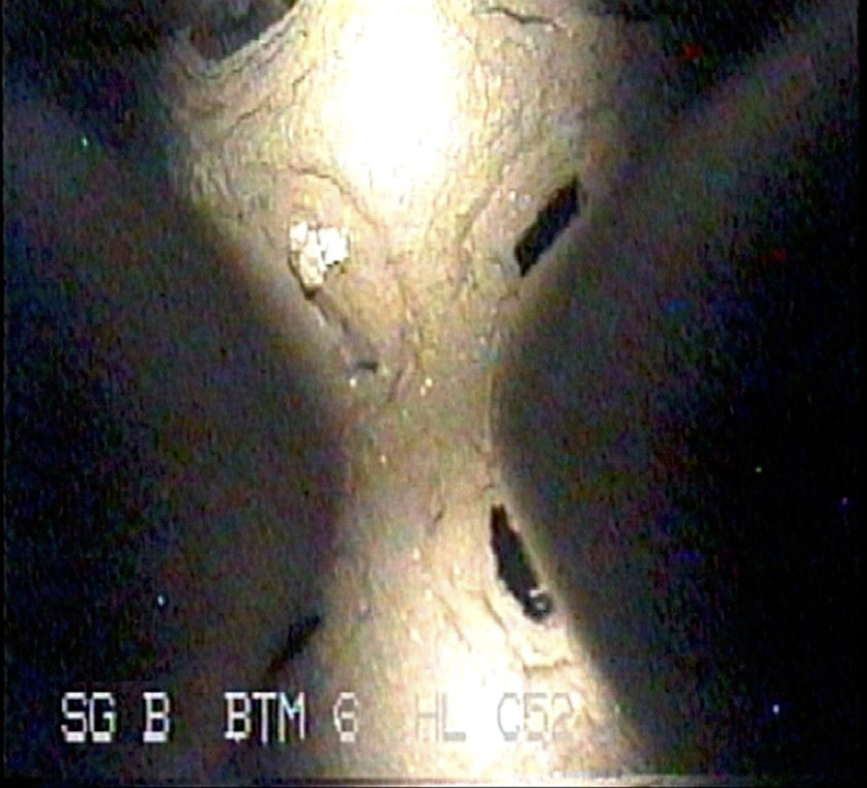
(A)	(B)
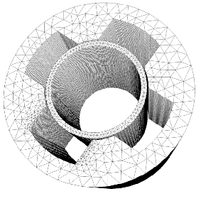
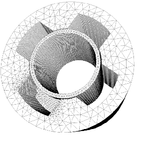
(A’)	(B’)

Fig. 2: Pictures downloaded from $\copyright$-Westinghouse: http://westinghousenuclear.com” . Figure (A) presents non clogging (healthy) SP, while Figure (B) presents a fully and partially clogged SP. Figures (A’)-(B’) are representations of used meshes for each configuration respectively.

Since the variational space (of the regularized variational formulation) is based on $H^{1}$ functions, the numerical finite elements approximation will be based on nodal finite elements for the electric vector potential $V$ as well as for the magnetic vector potential A. We shall mainly use $\mathbb{P}_{1}$ Lagrange nodal elements for both. In addition, the boundary conditions ($\textbf{A}\cdot\bm{n}=0$ on $\partial\Omega$) are taken into account via penalization of degrees of freedoms that belong to $\partial\Omega$. Indeed the same numerical approximation procedure is applied to adjoint states.

We now describe the gradient descent algorithm steps, the geometrical parametrizations and the procedure to accelerate iterations steps. The deposit is assumed to be located on the outer part of the tube and is concentrated (for the non axisymmetric examples) in one opening part of the SP (see Fig. 2-(B)). The reconstruction is based on an intuitive approach, which consists in iteratively P0-approximating the geometry of the deposit on a predefined 3D grid. This method avoid to reconstruct the mesh at each inversion iteration. The predefined grid is defined by $\mathcal{N}_{\underline{h}}=\{\mathcal{T}_{h}^{d}\subset\mathcal{T}_{h},\text{ s.t }\forall\text{ simplex }K\in\mathcal{T}_{h}^{d}\ \text{ with a facet parallel to Tube}\}$, where $\underline{h}$ stands for the resolution of the grid. We give in Fig. 3 a clipping of $\mathcal{N}_{\underline{h}}$.

Fig. 3: Sketch of the deposit shape reconstruction (clipping of 3D representation) on a grid $G_{\underline{h}}$. The reconstruction uses an invariant grid where P0-interpolation over this grid is set to cary out the new shape profile.

We present in Algorithm 1 the instances of an adapted step gradient descent. It is well known that the fixed step gradient descent algorithm converges if the step is sufficiently small. In our case we will allow the step descent to be large at least for the first iterations, and if the algorithm fails to maintain the decreasing of the cost functional, the step is reduced by a given factor. $1/2<\delta<1$. The final geometry is the one for which no local variation (on the predefined grid) decreases the cost functional.

Data: The impedance signal response of the tested configuration $\Omega_{d}^{\star}$

Result: Optimal shape approximation using interpolation on 3D grid

Input: The resolution of the predefined grid $\underline{h}$, ,Threshold: $\epsilon$

Input: $L^{0}$ Table of size $N$, a real $t$ and $\dfrac{1}{2}<\delta<1$

Input: $P=\mathrm{E}\big{(}log(0.4*\underline{h})/log(\delta)\big{)}$

1 Build the 3d mesh grid $\mathcal{N}_{\underline{h}}:m_{x}\underline{h}\times m_{y}\underline{h}\times N$

2 Evaluate the cost function $\mathbf{f}(L^{0})$ and the gradient $\nabla\mathbf{f}(L^{0})$

3 $k=0$

4 while $\|\nabla\mathbf{f}(L^{k})\|_{2}>\epsilon$ do

5       $t^{k}=\underline{h}/\max_{1\leq n\leq N}|\nabla\mathbf{f}(L_{n}^{k})|$

6       for $1\leq p\leq P$ do

7             $t^{p}=\delta\times t^{p-1}$

8             $L^{p}=L^{k}-t^{p}\nabla\mathbf{f}(L^{k})$

9             Project the $L^{p}$ (to the nearest value) on the predefined grid; Evaluate the cost function $\mathbf{f}(L^{p})$

10             if $\mathbf{f}(L^{p})<\mathbf{f}(L^{k})$ then

11                   Update $\mathbf{f}(L^{k+1})=\mathbf{f}(L^{p})$

12                   Evaluate the gradient $\nabla\mathbf{f}(L^{k+1})$

13                  

14                  Break

15                  

16             end if

17            if p==P then

18                   Print “A singular point is attained”

19                   Exit()

20                  

21             end if

22            

23       end for

24      

25      $k=k+1$

26      

27 end while

Algorithm 1 Gradient descent algorithm

5 Numerical implementation and validation

Numerical validation of the presented method is considered in this section. We use the software FreeFem++  [14] to deal with the finite elements discretization of the problem. We run our script on a cluster with distributed memory configuration. We use a direct matrix-inversion of the linear system where the factorization is achieved using sparse parallel solver (MUMPS [4, 5]). We present and explain in the sequel some particular techniques to achieve performance of the direct eddy-current solver (and consequently the inverse solver).

At each probe position we have to compute a solution associated to different source term. In order to (numerically) ensure divergence free condition for the source term one has to exactly mesh the support of the coil. If we build a new mesh related to the new probe position, we have to assemble new matrices and solve new systems, which are extremely memory-consuming. We therefore avoid this by creating and use a unique mesh that incorporates all possible probe positions in a scan of the tube. This allows us to only modify the right hand side of the system at each coil position. The factorization of the matrix is done only once per iteration. In order to further accelerate the resolution we also parallelize the matrix assembly since the cost of this part appeared to be the more expensive part if not done in parallel. Particular attention must be taken for the non-homogeneity (change of the conductivities and the permeability in the domain): We declare the variables $\sigma$ and $\mu$ as P0-Lagrange finite elements that depends on the elements labels of the non-partitioned mesh. Then, we apply a graph partitioning (e.g. scotch [24] or metis [19]) to create automatically partitioned new mesh. Since the partitioning process changes the elements labels to the ranks of the used group of processors, we define the P0-Lagrange non-homogeneous domain variable on the non-partitioned mesh and then include them in the variational formulation that admits the partitioning (see  [13] for more technical details).

Numerical experiments deal with several configurations of test cases. Mainly we present an axisymmetric configuration, then we add the SP and consider the case where one of the SP foils (flow path) is clogged.

The geometry of the computational domain includes a tube with respective internal and external radius $9.84$ mm and $11.11$ mm. The coils are modeled by a crown with respective internal and external radius $7.83$ mm and $8.50$ mm. Both coils have length $2$ mm and are separated by $0.5$ mm. The scan step of coils is fixed to $1$ mm and cover $20$ positions along the tube, which length has been limited to $30$ mm.

We used the following values of the electromagnetic parameters. The frequency $\omega=200\pi$, the magnetic permeability of the vacuum $\mu_{0}=\pi\times 10^{-6}$, magnetic permeability of the tube $\mu_{t}=1.01\mu_{0}$, the magnetic permeability of the SP $\mu_{SP}=\mu_{0}$ and the magnetic permeability of the deposit $\mu_{d}=\mu_{0}$. The conductivity is taken $\sigma_{t}=1\times 10^{3}$ for the tube, $\sigma_{SP}=1\times 10^{2}$ for the SP and $\sigma_{d}=\sigma_{t}$ for the deposit.

In all numerical experiments, the initialization of our algorithm takes a deposit with the lowest layers in the grid $G_{\underline{h}}$ i.e. with depth $0.5$ mm equal to ${\underline{h}}$ : the precision of the fixed grid.

5.1 Axisymmetric and non-axisymmetric geometries

In this part we consider two configurations of deposits in the vicinity of the tube: deposits around the tube far from SP and a deposit in one opening of water traffic lane of the SP. The first case, represents an axisymmetric configuration [18] and the second case represents a non-axisymmetric configuration because of the presence of SP and the deposit. We present in Figure 5 a slice on the plane (x,z) of the 3D computational domain. We show the shape of the axisymmetric deposits $\Omega_{d}^{\star}$ and the estimated deposits $\Omega_{d}^{k}$ result of the inversion algorithm. Together with this plot we add the y-component of the solution $\textbf{E}_{k}$ to show the penetration of the electromagnetic wave inside the tube and the deposits. With respect to $k$, a series of measured responses of the estimated deposit $\Omega_{d}^{k}$ is presented in Figure 4. This shows the convergence of the method in the sense of minimizing the misfit function (11) presented in Figure 6.

,

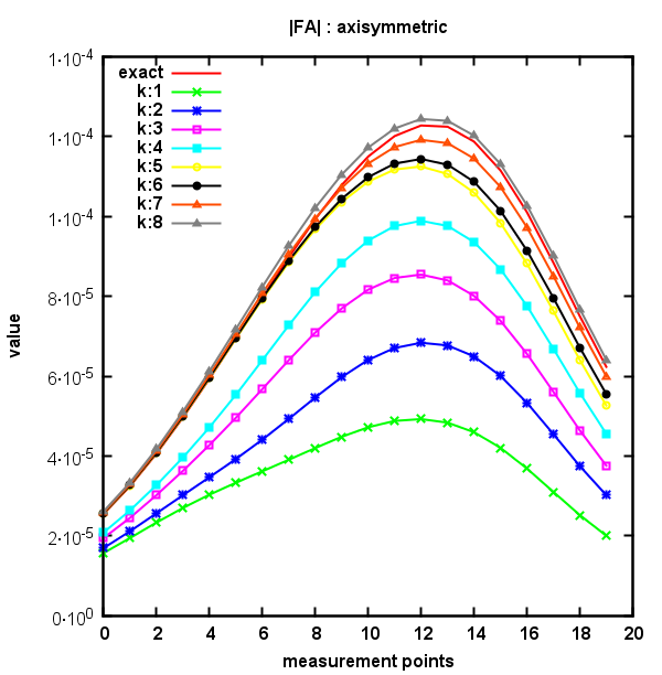
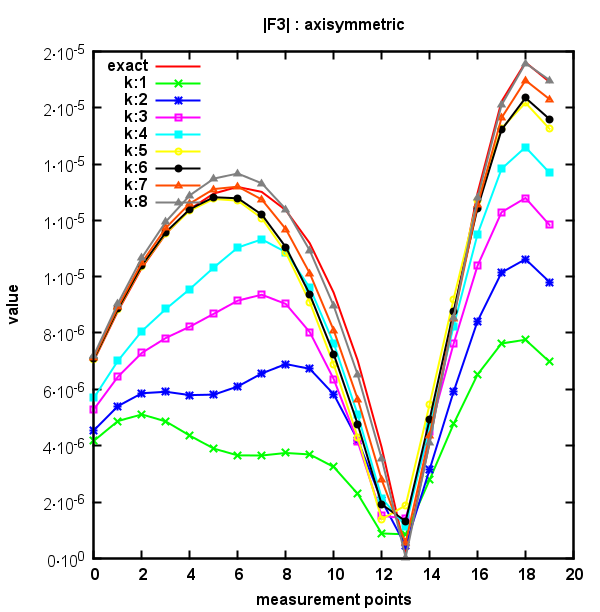
Fig. 4: History of the impedance responses of the deposits during iterations in the axisymmetric configuration. $|FA|$ measurements (left) and $|F3|$ measurements (right).

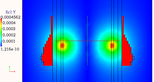
Fig. 5: Slice on x-z-plan of the computational domain showing the plot of the y-component of the eddy-current solution and the deposits $\Omega_{d}^{\star}$ (on the left) and the reconstruction in red (on the right).

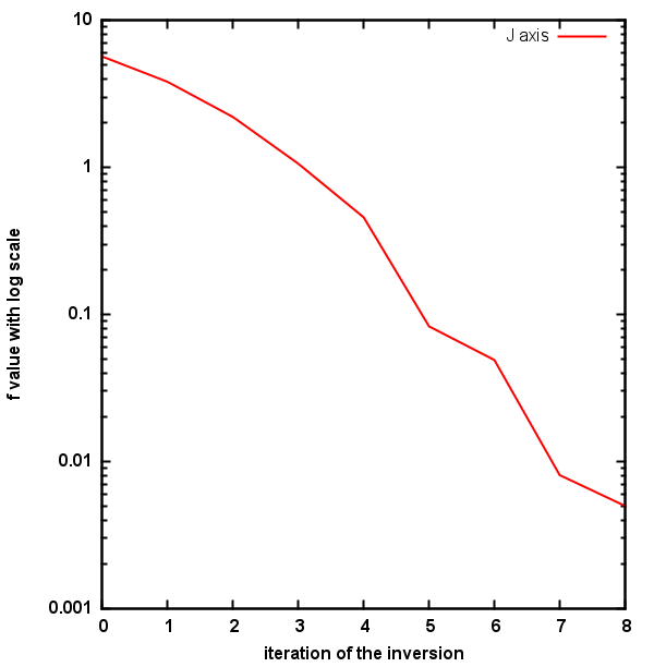
Fig. 6: Objective function with respect to iterations in the axisymmetric case.

A more complex configuration consists in taking into account the presence of SP and therefore non symmetric deposit. The results for this configuration are presented as follows: In Figure 8 we plot a slice, on the plane (x,z), of the y-component of the solution $\textbf{E}_{k}$ together with the shape profile of the deposits $\Omega_{d}^{\star}$ and its estimation $\Omega_{d}^{k}$ result of the inversion algorithm.

,

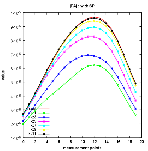
Fig. 7: History of the impedances during iterations for the SP configuration. $|FA|$ measurements (left) and $|F3|$ measurements (right).

The series of the impedance signal responses are given with respect to $k$ in Figure 7. This highlights the convergence of our algorithm even with the presence of noise in the non symmetric solution (y-component of $\textbf{E}_{k}$) as it can be seen in Figure 8 and also on the left plot of Figure 9.

Fig. 8: (left) Slice representation of the computational domain of the configuration with SP and a plot of the z-component of the eddy-current solution on x-y-plan. (right) Misfit function in terms of the inversion iterations.

Fig. 9: Slice representation of the computational domain of the configuration with SP and a plot of the y-component of the eddy-current solution on x-z-plan.

5.2 Arbitrary deposit shape

In this subsection in addition to the presence of the SP, we consider the reconstruction of a deposits with an arbitrary shape that does not match the parametrization used for the inverse problem: see Figure 10. The results of the inversion algorithm is given (in terms of $k$) in Figure 13. The convergence in the sense of the impedance response measurements is given in Figure 11. The minimization of the objective function with respect to the iterations of the inversion is presented in Figure 12.

Fig. 10: Graph of the arbitrary shaped deposit that clogs one opening (foils) of the tube SP.

,

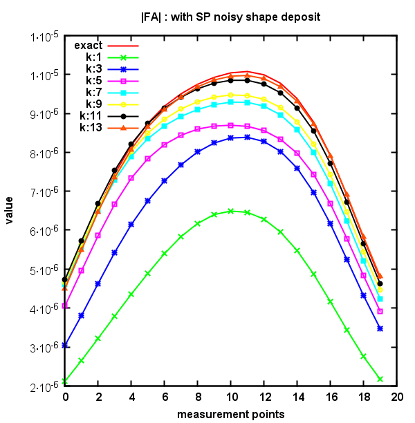
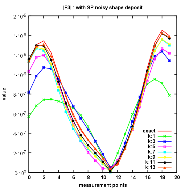
Fig. 11: History of the impedances in the case or deposit with arbitrary shape: $|FA|$ measurement (left) and $|F3|$ measurement (right).

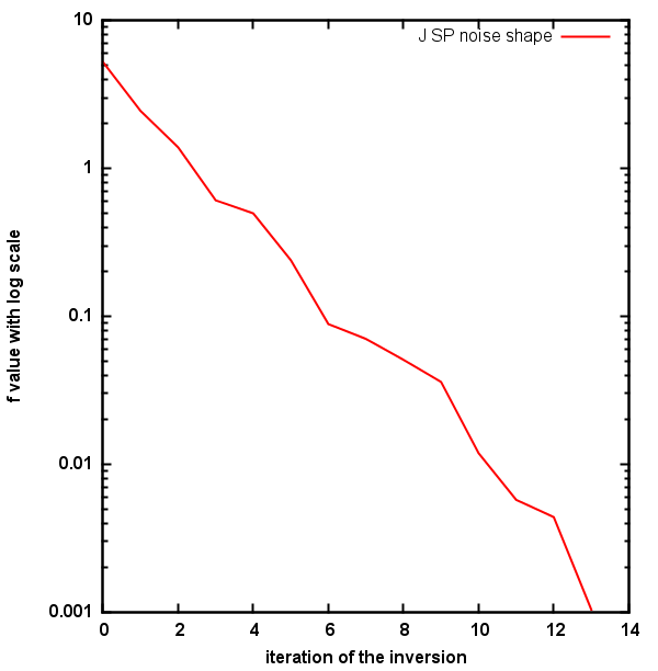
Fig. 12: Objective function with respect to iterations for the case of arbitrary shape reconstructions.

(k=0)	(k=2)	(k=4)
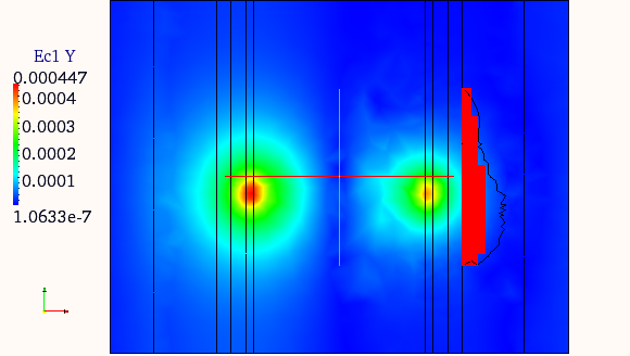
(k=6)	(k=8)	(k=10)
(k=11)	(k=12)	(k=13)

Fig. 13: Slice representation of the iterations of the shape reconstruction: case of an arbitrary shape clogging one opening of the quatrefoil SP.

Appendix A Some useful differential identities

(44a) $$\operatorname{curl}(\nabla f)=0,$$

(44b) $$\mathrm{div}\,(\operatorname{curl}\bm{v})=0,$$

(44c) $$(\bm{u}\cdot\nabla)\bm{v}=(\nabla\bm{v})\bm{u},$$

(44d) $$\operatorname{curl}\bm{u}\times\bm{v}=(\nabla\bm{u}-(\nabla\bm{u})^{t})\bm{v},$$

(44e) $$\nabla(\bm{u}\cdot\bm{v})=\bm{u}\times\operatorname{curl}\bm{v}+\bm{v}\times\operatorname{curl}\bm{u}+(\bm{u}\cdot\nabla)\bm{v}+(\bm{v}\cdot\nabla)\bm{u},$$

(44f) $$\operatorname{curl}(\bm{u}\times\bm{v})=\bm{u}\mathrm{div}\,\bm{v}-\bm{v}\mathrm{div}\,\bm{u}+(\bm{v}\cdot\nabla)\bm{u}-(\bm{u}\cdot\nabla)\bm{v}.$$

Appendix B Proof of Lemma 1

We develop the proof of the shape derivative calculus presented at Lemma 1

Proof.

By definition, one has

$$\mathsf{A}(\Omega_{\theta})\big{(}\textbf{A},V;\bm{\Psi},\Phi\big{)}= \int_{\Omega_{\theta}}\dfrac{1}{\mu}\operatorname{curl}_{y}\textbf{A}(\Omega_{\theta})\cdot\operatorname{curl}_{y}\overline{\bm{\Psi}(\Omega_{\theta})}\thinspace\mathrm{d}y$$

$$+\dfrac{1}{\mathrm{i}\omega}\int_{\Omega_{\theta}}\sigma(\mathrm{i}\omega\textbf{A}(\Omega_{\theta})+\nabla_{y}V(\Omega_{\theta}))\cdot(\overline{\mathrm{i}\omega\bm{\Psi}(\Omega_{\theta})+\nabla_{y}\Phi(\Omega_{\theta})})\thinspace\mathrm{d}y.$$

With the variable substitution $(\mathrm{Id}+\bm{\theta})^{-1}:y\mapsto x$ and the identities (12) related to $A_{\operatorname{curl}}$, $A_{\mathrm{div}\,}$ and $V_{\nabla}$, we rewrite the above form on a fixed reference domain $\Omega=(\mathrm{Id}+\bm{\theta})^{-1}\Omega_{\theta}$ as

$$\mathsf{A}(\Omega_{\theta})\big{(}\textbf{A},V;\bm{\Psi},\Phi\big{)}=\int_{\Omega}\dfrac{1}{\mu}\dfrac{(I+\nabla\bm{\theta})^{t}(I+\nabla\bm{\theta})}{|\det(I+\nabla\bm{\theta})|}\operatorname{curl}\textbf{A}_{\operatorname{curl}}\cdot\operatorname{curl}\overline{\bm{\Psi}_{\operatorname{curl}}}\thinspace\mathrm{d}x$$

$$+\dfrac{1}{\mathrm{i}\omega}\int_{\Omega}\sigma|\det(I+\nabla\bm{\theta})|(I+\nabla\bm{\theta})^{-1}(I+\nabla\bm{\theta})^{-t}\big{(}\mathrm{i}\omega\textbf{A}_{\operatorname{curl}}+\nabla V_{\nabla}\big{)}\cdot\big{(}\overline{\mathrm{i}\omega\bm{\Psi}_{\operatorname{curl}}+\nabla\Phi_{\nabla}}\big{)}\thinspace\mathrm{d}x.$$

If $(\textbf{B}(\bm{\theta}),U(\bm{\theta}))$, $(\bm{\eta}(\bm{\theta}),\chi(\bm{\theta}))$ are respectively the material derivatives of $(\textbf{A},V)$ and $(\bm{\Psi},\Phi)$, then one can develop the above form with respect to $\bm{\theta}$ by considering the developments [11]

(45a) $$|\det(I+\nabla\bm{\theta})|=1+\mathrm{div}\,\bm{\theta}+o(\bm{\theta}),$$

(45b) $$(I+\nabla\bm{\theta})^{-1}=I-\nabla\bm{\theta}+o(\bm{\theta}).$$

Since $(\textbf{A}_{\operatorname{curl}}(0),V_{\nabla}(0))=(\textbf{A}(\Omega),V(\Omega))$, $(\bm{\Psi}_{\operatorname{curl}}(0),\Phi_{\nabla}(0)=\Phi(\Omega))$, the terms of order zero with respect to $\bm{\theta}$ in the development give exactly $\mathsf{A}(\Omega)(\textbf{A},V;\bm{\Psi},\Phi)$, while the first order terms with respect to $\bm{\theta}$ yield

$$\mathsf{A}^{\prime}(\Omega)(\textbf{A},V;\bm{\Psi},\Phi)=\mathsf{A}(\Omega)(\textbf{B}(\bm{\theta}),U(\bm{\theta});\bm{\Psi},\Phi)+\mathsf{A}(\Omega)(\textbf{A},V;\bm{\eta}(\bm{\theta}),\chi(\bm{\theta}))+\mathcal{I}_{1}+\mathcal{I}_{2},$$

with $$\mathcal{I}_{1}=\int_{\Omega}\dfrac{1}{\mu}(-\mathrm{div}\,\bm{\theta}+\nabla\bm{\theta}+(\nabla\bm{\theta})^{t})\operatorname{curl}\textbf{A}\cdot\operatorname{curl}\overline{\bm{\Psi}}\thinspace\mathrm{d}x,$$

(46) $$\mathcal{I}_{2}=\dfrac{1}{\mathrm{i}\omega}\int_{\Omega}\sigma(\mathrm{div}\,\bm{\theta}I-\nabla\bm{\theta}-(\nabla\bm{\theta})^{t})\big{(}\mathrm{i}\omega\textbf{A}+\nabla V\big{)}\cdot\big{(}\overline{\mathrm{i}\omega\bm{\Psi}+\nabla\Phi}\big{)}\thinspace\mathrm{d}x.$$

We will rewrite the volume integrals $\mathcal{I}_{1}$, $\mathcal{I}_{2}$ in terms of boundary integrals. Using the differential identities (44) and the fact that $(\textbf{A},V)$ satisfy the conditions (20), one verifies

$$(-\mathrm{div}\,\bm{\theta}I+\nabla\bm{\theta}+(\nabla\bm{\theta})^{t})\operatorname{curl}\textbf{A}=-\operatorname{curl}((\bm{\theta}\cdot\nabla)\textbf{A}+(\nabla\theta)^{t}\textbf{A})+\nabla(\bm{\theta}\cdot\operatorname{curl}\textbf{A})+\mu\sigma(\mathrm{i}\omega\textbf{A}+\nabla V)\times\bm{\theta}.$$

Hence

$$\mathcal{I}_{1}=-\int_{\Omega}\dfrac{1}{\mu}\operatorname{curl}((\bm{\theta}\cdot\nabla)\textbf{A}+(\nabla\theta)^{t}\textbf{A})\cdot\operatorname{curl}\overline{\bm{\Psi}}\thinspace\mathrm{d}x+\mathcal{I}_{11}+\mathcal{I}_{22},$$

$$\text{where}\quad\mathcal{I}_{11}=\int_{\Omega}\dfrac{1}{\mu}\nabla(\bm{\theta}\cdot\operatorname{curl}\textbf{A})\cdot\operatorname{curl}\overline{\bm{\Psi}}\thinspace\mathrm{d}x\quad\text{and}\quad\mathcal{I}_{12}=\int_{\Omega}\sigma\big{(}(\mathrm{i}\omega\textbf{A}+\nabla V)\times\bm{\theta}\big{)}\cdot\operatorname{curl}\overline{\bm{\Psi}}\thinspace\mathrm{d}x.$$

By Stoke’s theorem, one has

$$\mathcal{I}_{11}=\int_{\Omega}\dfrac{1}{\mu}\mathrm{div}\,\big{(}(\bm{\theta}\cdot\operatorname{curl}\textbf{A})\operatorname{curl}\overline{\bm{\Psi}}\big{)}\thinspace\mathrm{d}x=\int_{\partial\Omega}\dfrac{1}{\mu}(\bm{\theta}\cdot\operatorname{curl}\textbf{A})(\bm{n}\cdot\operatorname{curl}\overline{\bm{\Psi}})\thinspace\mathrm{d}s.$$

By integration by parts (with use of differential identities 44), we verify

$$\mathcal{I}_{12}= -\dfrac{1}{\mathrm{i}\omega}\int_{\Omega}\sigma\big{\{}(\mathrm{div}\,\bm{\theta}I-\nabla\bm{\theta})(\mathrm{i}\omega\textbf{A}+\nabla V)+(\bm{\theta}\cdot\nabla)(\mathrm{i}\omega\textbf{A}+\nabla V)\big{\}}\cdot(\overline{\mathrm{i}\omega\bm{\Psi}})\thinspace\mathrm{d}x$$

$$+\dfrac{1}{\mathrm{i}\omega}\int_{\partial\Omega}\sigma(\bm{\theta}\cdot\bm{n})(\mathrm{i}\omega\textbf{A}+\nabla V)\cdot(\overline{\mathrm{i}\omega\bm{\Psi}})\thinspace\mathrm{d}s.$$

Therefore

$$\mathcal{I}_{1}= -\int_{\Omega}\dfrac{1}{\mu}\operatorname{curl}((\bm{\theta}\cdot\nabla)\textbf{A}+(\nabla\theta)^{t}\textbf{A})\cdot\operatorname{curl}\overline{\bm{\Psi}}\thinspace\mathrm{d}x$$

$$-\dfrac{1}{\mathrm{i}\omega}\int_{\Omega}\sigma\big{\{}(\mathrm{div}\,\bm{\theta}I-\nabla\bm{\theta})(\mathrm{i}\omega\textbf{A}+\nabla V)+(\bm{\theta}\cdot\nabla)(\mathrm{i}\omega\textbf{A}+\nabla V)\big{\}}\cdot(\overline{\mathrm{i}\omega\bm{\Psi}})\thinspace\mathrm{d}x$$

(47) $$+\int_{\partial\Omega}\dfrac{1}{\mu}(\bm{\theta}\cdot\operatorname{curl}\textbf{A})(\bm{n}\cdot\operatorname{curl}\overline{\bm{\Psi}})\thinspace\mathrm{d}s+\dfrac{1}{\mathrm{i}\omega}\int_{\partial\Omega}\sigma(\bm{\theta}\cdot\bm{n})(\mathrm{i}\omega\textbf{A}+\nabla V)\cdot(\overline{\mathrm{i}\omega\bm{\Psi}})\thinspace\mathrm{d}s.$$

Now we compute the term $\mathcal{I}_{2}$

$$\mathcal{I}_{2}=\dfrac{1}{\mathrm{i}\omega}\int_{\Omega}\sigma(\mathrm{div}\,\bm{\theta}I-\nabla\bm{\theta}-(\nabla\bm{\theta})^{t})(\mathrm{i}\omega\textbf{A}+\nabla V)\cdot(\overline{\mathrm{i}\omega\bm{\Psi}})\thinspace\mathrm{d}x+\mathcal{I}_{21}+\mathcal{I}_{22},$$

with $$\mathcal{I}_{21}=\dfrac{1}{\mathrm{i}\omega}\int_{\Omega}\sigma\mathrm{div}\,\bm{\theta}(\mathrm{i}\omega\textbf{A}+\nabla V)\cdot\nabla\overline{\Phi}\thinspace\mathrm{d}x,\quad\mathcal{I}_{22}=\dfrac{1}{\mathrm{i}\omega}\int_{\Omega}\sigma(-\nabla\bm{\theta}-(\nabla\bm{\theta})^{t})(\mathrm{i}\omega\textbf{A}+\nabla V)\cdot\nabla\overline{\Phi}\thinspace\mathrm{d}x.$$

By integration by parts, one obtains

$$\mathcal{I}_{21}= \dfrac{1}{\mathrm{i}\omega}\int_{\partial\Omega}\sigma(\bm{\theta}\cdot\bm{n})(\mathrm{i}\omega\textbf{A}+\nabla V)\cdot\nabla\overline{\Phi}\thinspace\mathrm{d}s-\dfrac{1}{\mathrm{i}\omega}\int_{\Omega}\mathrm{i}\omega\sigma(\bm{\theta}\cdot\nabla)\textbf{A}\cdot\nabla\overline{\Phi}\thinspace\mathrm{d}x$$

$$-\dfrac{1}{\mathrm{i}\omega}\int_{\Omega}\sigma D^{2}\overline{\Phi}(\mathrm{i}\omega\textbf{A}+\nabla V)\cdot\bm{\theta}\thinspace\mathrm{d}x-\dfrac{1}{\mathrm{i}\omega}\int_{\Omega}\sigma D^{2}V\bm{\theta}\cdot\nabla\overline{\Phi}\thinspace\mathrm{d}x.$$

Using integration by parts and the fact that $\mathrm{div}\,(\sigma(\mathrm{i}\omega\textbf{A}+\nabla V))=0$ obtained by applying the divergence operator to (20)₁, one verifies

$$\mathcal{I}_{22}= -\dfrac{1}{\mathrm{i}\omega}\int_{\Omega}\sigma(\nabla\bm{\theta})^{t}(\mathrm{i}\omega\textbf{A}+\nabla V)\cdot\nabla\overline{\Phi}\thinspace\mathrm{d}x+\dfrac{1}{\mathrm{i}\omega}\int_{\Omega}D^{2}\overline{\Phi}(\mathrm{i}\omega\textbf{A}+\nabla V)\cdot\bm{\theta}\thinspace\mathrm{d}x.$$

From the differential identities (44), one deduces also that

$$D^{2}V\bm{\theta}+(\nabla\bm{\theta})^{t}\nabla V=(\bm{\theta}\cdot\nabla)\nabla V+(\nabla\bm{\theta})^{t}\nabla V=\nabla(\bm{\theta}\cdot\nabla V).$$

The above equalities yield

$$\mathcal{I}_{2}= \mathcal{I}_{21}+\mathcal{I}_{22}$$

$$= \dfrac{1}{\mathrm{i}\omega}\int_{\Omega}\sigma(\mathrm{div}\,\bm{\theta}I-\nabla\bm{\theta}-(\nabla\bm{\theta})^{t})(\mathrm{i}\omega\textbf{A}+\nabla V)\cdot(\overline{\mathrm{i}\omega\bm{\Psi}})\thinspace\mathrm{d}x+\dfrac{1}{\mathrm{i}\omega}\int_{\partial\Omega}\sigma(\bm{\theta}\cdot\bm{n})(\mathrm{i}\omega\textbf{A}+\nabla V)\cdot\nabla\overline{\Phi}\thinspace\mathrm{d}s$$

(48) $$-\dfrac{1}{\mathrm{i}\omega}\int_{\Omega}\sigma\mathrm{i}\omega\big{(}(\bm{\theta}\cdot\nabla)\textbf{A}+(\nabla\bm{\theta})^{t}\textbf{A}\big{)}\cdot\nabla\overline{\Phi}\thinspace\mathrm{d}x-\dfrac{1}{\mathrm{i}\omega}\int_{\Omega}\sigma\nabla(\bm{\theta}\cdot\nabla V)\cdot\nabla\overline{\Phi}\thinspace\mathrm{d}x.$$

(B), (B) and the fact that $\sigma(\mathrm{i}\omega\textbf{A}+\nabla V)\cdot\bm{n}=0$ on $\partial\Omega$ imply

$$\mathcal{I}_{1}+\mathcal{I}_{2}= \mathsf{A}(\Omega)\Big{(}-(\bm{\theta}\cdot\nabla)\textbf{A}-(\nabla\theta)^{t}\textbf{A},-(\bm{\theta}\cdot\nabla V);\bm{\Psi},\Phi\Big{)}$$

(49) $$+\int_{\partial\Omega}\dfrac{1}{\mu}(\bm{\theta}\cdot\operatorname{curl}\textbf{A})(\bm{n}\cdot\operatorname{curl}\overline{\bm{\Psi}})\thinspace\mathrm{d}s+\dfrac{1}{\mathrm{i}\omega}\int_{\partial\Omega}\sigma(\bm{\theta}\cdot\bm{n})(\mathrm{i}\omega\textbf{A}_{\tau}+\nabla_{\tau}v)\cdot(\overline{\mathrm{i}\omega\bm{\Psi}_{\tau}+\nabla\Phi_{\tau}})\thinspace\mathrm{d}s.$$

From (B), (B) and the definition of shape derivatives (14), one concludes the result (21). ∎

Appendix C Proof of Proposition 6

We give the proof of the stated theorem 6

Proof.

Taking $(\bm{\Psi},\Phi)=(\textbf{B}_{k}(\bm{\theta}),U_{k}(\bm{\theta}))\in\mathcal{Q}$ in the adjoint problem (39) yields

$$\mathcal{S}^{*}(\textbf{P}_{l},W_{l};\textbf{B}_{k}(\bm{\theta}),U_{k}(\bm{\theta}))=L^{*}(\textbf{B}_{k}(\bm{\theta}),U_{k}(\bm{\theta})).$$

On the other hand, taking $(\bm{\varPsi},\varPhi)=(\textbf{P}_{l},W_{l})$ in the variational formulation (29) for the material derivatives $(\textbf{B}_{k}(\bm{\theta}),U_{k}(\bm{\theta}))$ implies

$$\mathcal{S}(\textbf{B}_{k}(\bm{\theta}),U_{k}(\bm{\theta});\textbf{P}_{l},W_{l})=\mathcal{L}(\textbf{P}_{l},W_{l}).$$

Since

$$\overline{\mathcal{S}^{*}(\textbf{P}_{l},W_{l};\textbf{B}_{k}(\bm{\theta}),U_{k}(\bm{\theta}))}=\mathcal{S}(\textbf{B}_{k}(\bm{\theta}),U_{k}(\bm{\theta});\textbf{P}_{l},W_{l})$$

with the fact that $\mathrm{div}\,\textbf{P}_{l}=0$, one obtains

$$\overline{L^{*}(\textbf{B}_{k}(\bm{\theta}),U_{k}(\bm{\theta}))}=\mathcal{L}(\textbf{P}_{l},W_{l}).$$

$$=\int_{\Omega_{d}}\dfrac{1}{\mu}\operatorname{curl}\big{(}(\bm{\theta}\cdot\nabla)\textbf{A}_{k}+(\nabla\bm{\theta})^{t}\textbf{A}_{k}\big{)}\cdot\operatorname{curl}\overline{\textbf{P}_{l}}\thinspace\mathrm{d}x$$

$$+\dfrac{1}{\mathrm{i}\omega}\int_{\Omega_{\mathcal{C}}}\sigma\bigg{(}\mathrm{i}\omega\big{(}(\bm{\theta}\cdot\nabla)\textbf{A}_{k}+(\nabla\bm{\theta})^{t}\textbf{A}_{k}\big{)}+\nabla(\bm{\theta}\cdot\nabla V_{k})\bigg{)}\cdot(\overline{\mathrm{i}\omega\textbf{P}_{l}+\nabla W_{l}})\thinspace\mathrm{d}x$$

$$+\int_{\Gamma}\left[\dfrac{1}{\mu}\right](\bm{\theta}\cdot\bm{n})(\bm{n}\cdot\operatorname{curl}\textbf{A}_{k})(\bm{n}\cdot\operatorname{curl}\overline{\textbf{P}_{l}})\thinspace\mathrm{d}s+\dfrac{1}{\mathrm{i}\omega}\int_{\Gamma}(\bm{\theta}\cdot\bm{n})[\sigma](\mathrm{i}\omega\textbf{A}_{k\tau}+\nabla_{\tau}V_{k})\cdot(\overline{\mathrm{i}\omega\textbf{P}_{l\tau}+\nabla_{\tau}W_{l}})\thinspace\mathrm{d}s.$$

In $\Omega\backslash\Gamma$ one verifies

$$(\bm{\theta}\cdot\nabla)\textbf{A}_{k}+(\nabla\bm{\theta})^{t}\textbf{A}_{k}=\operatorname{curl}\textbf{A}_{k}\times\bm{\theta}+\nabla(\bm{\theta}\cdot\textbf{A}_{k}),$$

$$\operatorname{curl}\big{(}(\bm{\theta}\cdot\nabla)\textbf{A}_{k}+(\nabla\bm{\theta})^{t}\textbf{A}_{k}\big{)}=\operatorname{curl}\big{(}\operatorname{curl}\textbf{A}_{k}\times\bm{\theta}\big{)}.$$

Thus, considering (40)₄ and (40)₅, we compute

$$\overline{L^{*}(\textbf{B}_{k}(\bm{\theta}),U_{k}(\bm{\theta}))}$$

$$=\mathcal{I}+\int_{\Gamma}\left[\dfrac{1}{\mu}\right](\bm{\theta}\cdot\bm{n})(\bm{n}\cdot\operatorname{curl}\textbf{A}_{k})(\bm{n}\cdot\operatorname{curl}\overline{\textbf{P}_{l}})\thinspace\mathrm{d}s+\dfrac{1}{\mathrm{i}\omega}\int_{\Gamma}(\bm{\theta}\cdot\bm{n})[\sigma](\mathrm{i}\omega\textbf{A}_{k\tau}+\nabla_{\tau}V_{k})\cdot(\overline{\mathrm{i}\omega\textbf{P}_{l\tau}+\nabla_{\tau}W_{l}})\thinspace\mathrm{d}s,$$

(50) $$\text{with}\quad\mathcal{I}=\int_{\Omega_{d}}\dfrac{1}{\mu}\operatorname{curl}\big{(}\operatorname{curl}\textbf{A}_{k}\times\bm{\theta}\big{)}\cdot\operatorname{curl}\overline{\textbf{P}_{l}}\thinspace\mathrm{d}x+\dfrac{1}{\mathrm{i}\omega}\int_{\Omega_{\mathcal{C}}}\sigma\mathrm{i}\omega\big{(}\operatorname{curl}\textbf{A}_{k}\times\bm{\theta}\big{)}\cdot(\overline{\mathrm{i}\omega\textbf{P}_{l}+\nabla W_{l}})\thinspace\mathrm{d}x.$$

We remind that $(\operatorname{curl}\textbf{A}_{k}\times\bm{\theta})$ belongs to $X(\Omega)$. We multiply (40)₁ by $\big{(}\overline{\operatorname{curl}A_{k}\times\bm{\theta}}\big{)}$, integrate by parts and then take the complex conjugate, which implies

$$\mathcal{I} =\int_{\Omega_{d}}(\dfrac{1}{\mu}-\dfrac{1}{\mu^{0}})\operatorname{curl}\textbf{A}_{l}^{0}\cdot\operatorname{curl}(\operatorname{curl}\textbf{A}_{k}\times\bm{\theta})\thinspace\mathrm{d}x-\dfrac{1}{\mathrm{i}\omega}\int_{\Omega_{d}}[\sigma](\mathrm{i}\omega\textbf{A}_{l}^{0}+\nabla V_{l}^{0})\cdot\big{(}\mathrm{i}\omega(\operatorname{curl}A_{k}\times\bm{\theta})\big{)}\thinspace\mathrm{d}x$$

$$\quad+\int_{\Gamma}\left[\dfrac{1}{\mu}\operatorname{curl}\overline{\textbf{P}_{l}}\cdot\big{(}(\operatorname{curl}\textbf{A}_{k}\times\bm{\theta})\times\bm{n}\big{)}\right]\thinspace\mathrm{d}s+\int_{\Gamma}\left[\dfrac{1}{\mu}\right]\operatorname{curl}\overline{\textbf{A}_{l}^{0}}\cdot\big{(}(\operatorname{curl}\textbf{A}_{k}\times\bm{\theta})\times\bm{n}\big{)}\thinspace\mathrm{d}s$$

$$=\int_{\Omega_{d}}\left[\dfrac{1}{\mu}\right]\operatorname{curl}\textbf{A}_{l}^{0}\cdot\operatorname{curl}\big{(}(\bm{\theta}\cdot\nabla)\textbf{A}_{k}+(\nabla\bm{\theta})^{t}\textbf{A}_{k}\big{)}\thinspace\mathrm{d}x$$

$$\quad-\dfrac{1}{\mathrm{i}\omega}\int_{\Omega_{d}}[\sigma](\mathrm{i}\omega\textbf{A}_{l}^{0}+\nabla V_{l}^{0})\cdot\bigg{(}\mathrm{i}\omega\big{(}(\bm{\theta}\cdot\nabla)\textbf{A}_{k}+(\nabla\bm{\theta})^{t}\textbf{A}_{k}\big{)}+\nabla(\bm{\theta}\cdot\nabla V_{k})\bigg{)}\thinspace\mathrm{d}x$$

(51) $$\quad-\int_{\Gamma}(\bm{\theta}\cdot\bm{n})[\mu]\left(\dfrac{1}{\mu}\operatorname{curl}\textbf{A}_{k}\times\bm{n}\right)\cdot\left(\dfrac{1}{\mu^{0}}(\operatorname{curl}\overline{\textbf{P}_{l}})_{+}\times\bm{n}\right)\thinspace\mathrm{d}s$$

The last equality is due to the transmission conditions (40)₂ – (40)₃ for $\textbf{P}_{l}$ and those for $\textbf{A}_{k}$ on $\Gamma$: $[\bm{n}\cdot\operatorname{curl}\textbf{A}]=[\mu^{-1}\bm{n}\times\operatorname{curl}\textbf{A}]=0$. (C) and (C) imply

$$\overline{L^{*}(\textbf{B}_{k}(\bm{\theta}),U_{k}(\bm{\theta}))}-\int_{\Omega_{d}}\left[\dfrac{1}{\mu}\right]\operatorname{curl}\textbf{A}_{l}^{0}\cdot\operatorname{curl}\big{(}(\bm{\theta}\cdot\nabla)\textbf{A}_{k}+(\nabla\bm{\theta})^{t}\textbf{A}_{k}\big{)}\thinspace\mathrm{d}x$$

$$\quad+\dfrac{1}{\mathrm{i}\omega}\int_{\Omega_{d}}[\sigma](\mathrm{i}\omega\textbf{A}_{l}^{0}+\nabla V_{l}^{0})\cdot\bigg{(}\mathrm{i}\omega\big{(}(\bm{\theta}\cdot\nabla)\textbf{A}_{k}+(\nabla\bm{\theta})^{t}\textbf{A}_{k}\big{)}+\nabla(\bm{\theta}\cdot\nabla V_{k})\bigg{)}\thinspace\mathrm{d}x$$

$$=\int_{\Gamma}(\bm{\theta}\cdot\bm{n})\bigg{\{}\left[\dfrac{1}{\mu}\right](\bm{n}\cdot\operatorname{curl}\textbf{A}_{k})(\bm{n}\cdot\operatorname{curl}\overline{\textbf{P}_{l}})-[\mu]\left(\dfrac{1}{\mu}\operatorname{curl}\textbf{A}_{k}\times\bm{n}\right)\cdot\left(\dfrac{1}{\mu^{0}}(\operatorname{curl}\overline{\textbf{P}_{l}})_{+}\times\bm{n}\right)$$

(52) $$\qquad\qquad\qquad+\dfrac{1}{\mathrm{i}\omega}[\sigma](\mathrm{i}\omega\textbf{A}_{k\tau}+\nabla_{\tau}V_{k})\cdot(\overline{\mathrm{i}\omega\textbf{P}_{l\tau}+\nabla_{\tau}W_{l}})\bigg{\}}\thinspace\mathrm{d}s.$$

Considering the definition of $L^{*}(\cdot,\cdot)$, we substitute the above integral (C) in the expression of shape derivative of $\triangle Z_{kl}$ (3.3) and finally obtain (6). ∎

References

• [1] R. Albanese and P. B. Monk. The inverse source problem for Maxwell’s equations. Inverse Problems, 22(3):1023–1035, 2006.
• [2] Ana Alonso Rodríguez and Alberto Valli. Eddy current approximation of Maxwell equations, volume 4 of MS&A. Modeling, Simulation and Applications. Springer-Verlag Italia, Milan, 2010. Theory, algorithms and applications.
• [3] Ana Alonso Rodríguez, Jessika Camaño, and Alberto Valli. Inverse source problems for eddy current equations. Inverse Problems, 28(1):015006, 2012.
• [4] P. R. Amestoy, I. S. Duff, J. Koster, and J.-Y. L’Excellent. A fully asynchronous multifrontal solver using distributed dynamic scheduling. SIAM Journal on Matrix Analysis and Applications, 23(1):15–41, 2001.
• [5] P. R. Amestoy, A. Guermouche, J.-Y. L’Excellent, and S. Pralet. Hybrid scheduling for the parallel solution of linear systems. Parallel Computing, 32(2):136–156, 2006.
• [6] L. Arnold and B. Harrach. Unique shape detection in transient eddy current problems. Inverse Problems, 29(9):095004, 19, 2013.
• [7] BA Auld and JC Moulder. Review of advances in quantitative eddy current nondestructive evaluation. Journal of Nondestructive evaluation, 18(1):3–36, 1999.
• [8] Aniss Bendjoudi, Emmanuel Bossy, Marie-Françoise Cugnet, Patrick Chauvin, and Didier Cassereau. Développement d’un logiciel hybride pour le Contrôle Non Destructif. In Société Française d’Acoustique SFA, editor, 10ème Congrès Français d’Acoustique, pages –, Lyon, France, 2010.
• [9] John Cagnol and Matthias Eller. Shape optimization for the Maxwell equations under weaker regularity of the data. C. R. Math. Acad. Sci. Paris, 348(21-22):1225–1230, 2010.
• [10] The Open Access NDT Database. The web’s largest database of nondestructive testing (ndt) conference proceedings, articles, news, exhibition, forum and a professional network. NDT Database and Journal of Nondestructive Testing - NDT, Ultrasonic Testing, X-Ray, Radiography, Eddy Current and All NDT Methods., 2014.
• [11] M De Schoenauer and Grégoire Allaire. Conception optimale de structures, volume 58. Springer Science & Business, 2006.
• [12] H Griffiths. Magnetic induction tomography. Measurement science and technology, 12(8):1126, 2001.
• [13] Houssem Haddar and Mohamed Kamel Riahi. 3D direct and inverse solvers for eddy current testing of deposits in steam generator. Technical report for Lab STEP of French electricity company EDF, July 2013.
• [14] F. Hecht. New development in freefem++. J. Numer. Math., 20(3-4):251–265, 2012.
• [15] Frank Hettlich. The domain derivative of time-harmonic electromagnetic waves at interfaces. Math. Methods Appl. Sci., 35(14):1681–1689, 2012.
• [16] Haoyu Huang, T. Takagi, and H. Fukutomi. Fast signal predictions of noised signals in eddy current testing. Magnetics, IEEE Transactions on, 36(4):1719–1723, Jul 2000.
• [17] Haoyu Huang and Toshiyuki Takagi. Crack shape reconstruction from noisy signals in ect of steam generator tube. In Industrial Electronics Society, 2000. IECON 2000. 26th Annual Confjerence of the IEEE, volume 4, pages 2507–2512. IEEE, 2000.
• [18] Zixian Jiang, Mabrouka El-Guedri, Houssem Haddar, and Armin Lechleiter. Eddy current tomography of deposits in steam generator. In 2011 EUSIPCO Proc, pages 2054–2058, Barcelona, Spain, 2011.
• [19] George Karypis and Vipin Kumar. Metis - unstructured graph partitioning and sparse matrix ordering system, version 2.0, 1995.
• [20] H.-J. Krause, G.I. Panaitov, and Yi Zhang. Conductivity tomography for non-destructive evaluation using pulsed eddy current with hts squid magnetometer. Applied Superconductivity, IEEE Transactions on, 13(2):215–218, June 2003.
• [21] Leo Mariappan, Gang Hu, and Bin He. Magnetoacoustic tomography with magnetic induction for high-resolution bioimepedance imaging through vector source reconstruction under the static field of mri magnet. Medical Physics, 41(2):–, 2014.
• [22] Peter Monk. Finite element methods for Maxwell’s equations. Numerical Mathematics and Scientific Computation. Oxford University Press, New York, 2003.
• [23] Stephen J. Norton and John R. Bowler. Theory of eddy current inversion. Journal of Applied Physics, 73(2):501–512, 1993.
• [24] François Pellegrini. Scotch and libscotch 3.4 user’s guide, 2001.
• [25] Toshiyuki Takagi, Junji Tani, Hiroyuki Fukutomi, and Mitsuo Hashimoto. Finite element modeling of eddy current testing of steam generator tube with crack and deposit. In DonaldO. Thompson and DaleE. Chimenti, editors, Review of Progress in Quantitative Nondestructive Evaluation, volume 16 of Review of Progress in Quantitative Nondestructive Evaluation, pages 263–270. Springer US, 1997.
• [26] Gui Yun Tian, A. Sophian, D. Taylor, and J. Rudlin. Multiple sensors on pulsed eddy-current detection for 3-d subsurface crack assessment. Sensors Journal, IEEE, 5(1):90–96, Feb 2005.