A Different View on the Vector-valued
Empirical Mode Decomposition (VEMD)

Abstract

The empirical mode decomposition (EMD) has achieved its reputation by providing a multi-scale time-frequency representation of nonlinear and/or nonstationary signals. To extend this method to vector-valued signals (VvS) in multi-dimensional (multi-D) space, a multivariate EMD (MEMD) has been designed recently, which employs an ensemble projection to extract local extremum locations (LELs) of the given VvS with respect to different projection directions. This idea successfully overcomes the problems of locally defining extrema of VvS. Different from the MEMD, where vector-valued envelopes (VvEs) are interpolated based on LELs extracted from the 1-D projected signal, the vector-valued EMD (VEMD) proposed in this paper employs a novel back projection method to interpolate the VvEs from 1-D envelopes in the projected space. Considering typical 4-D coordinates (3-D location and time), we show by numerical simulations that the VEMD outperforms state-of-art methods.

I Introduction

The empirical mode decomposition (EMD) was firstly designed for nonlinear and/or nonstationary signal analysis [1]. Combined with the Hilbert transform, the Hilbert-Huang-Transform (HHT) [2] provides a finer time-frequency spectrum of a given signal compared with other well-known methods such as the Fourier transform, the wavelet transform, or the Wigner-Ville transform. Moreover, the EMD does not require any pre-defined basis. It decomposes a given signal $f(t)$ into a finite number of intrinsic mode functions (IMFs), $f_{j}(t):=a_{j}(t)\cos(\theta_{j}(t)),j=1,\ldots,J$, and a monotonic trend $r_{J+1}(t)$, i.e.,

$$f(t):=\sum_{j=1}^{J}f_{j}(t)+r_{J+1}(t),\qquad t\in[0,T].$$ (1)

Here, each $f_{j}(t)$ might be considered as an amplitude-modulated and frequency-modulated signal, or as a generalized Fourier component [3]. The properties of the signal model are extensively studied in [1, 4] and the references therein. Based on (1), the instantaneous frequency of each IMF is well defined by ${\omega}_{j}(t):=\theta^{\prime}_{j}(t)$ [5]. In addition, the corresponding Hilbert amplitude spectrum can be naturally derived as $\{a_{j}(t)\mbox{ on the curves }(t,\omega_{j}(t)),~{}t\in[0,T],~{}j=1,\ldots,J\}$ [4]. Up to now, the EMD and its many variations have been successfully employed in many disciplines, such as signal processing [2], hydrology [6], and geophysics [7].

In general, the EMD aims at sequentially extracting each IMF $f_{j}(t)$ through a filtering operation called sifting process. Considering the signal at the $k$th level, $x_{k}(t):=f(t)-\sum_{j=1}^{k-1}f_{j}(t)$, the sifting operator ${\mathcal{S}}$ can recursively be defined by ${\mathcal{S}}^{n}[x_{k}](t):={\mathcal{S}}^{n-1}[x_{k}](t)-{\mathcal{M}}[{\mathcal{S}}^{n-1}[x_{k}]](t)$, where $n$ is the iteration number, ${\mathcal{S}}^{0}[x_{k}](t):=x_{k}(t)$, and ${\mathcal{M}}[\cdot]$ represents the local trend approximation operator. In the classic EMD [1], ${\mathcal{M}}[x](t)$ is defined as the mean curve of the upper and lower envelopes which are defined by cubic spline interpolation of the local maxima and local minima of $x(t)$, respectively. The sifting process stops at $n=N$ until some ad hoc criterion is met, e.g. $f_{k}(t):={\mathcal{S}}^{N}[x_{k}](t)$ mimics in some sense a generalized Fourier component.

The EMD is a completely data-driven decomposition method which heavily depends on the definition of local extrema. Since their definition is unclear in higher dimensions, or the extrema are nonunique, it is, therefore, difficult to extend the method to these cases. The original signal or univariate time series decomposed in (1) consisted of data of the form $f:[0,T]\to{\mathbb{R}}$, mapping one-dimensional data in one-dimensional space. In higher dimensions, we distinguish between multivariate and vector-valued data. The multivariate case consists of ‘cube’ data, e.g., an image in 2-D, or a volume in 3-D. In this case, the function is of the form $f:[0,T]^{d}\to{\mathbb{R}}$ with $d=2,3$ being the space dimension. Here, a local extremum may be defined as the strict extremum in a pre-defined neighborhood [8]. However, in the vector-valued case, the data are multi-D ‘curve’ data which are of the form $f:[0,T]\to{\mathbb{R}}^{d}$. In this case, the definition of local extrema is much more complicated since even the notion of ‘neighborhood’ is unclear.

In this paper, we concentrate on the latter, more difficult, case. We define the vector-valued signal as follows.

Definition I.1

Given a finite number of 1-D signals $f^{[i]}(t)\in C({\mathbb{R}})\cap L_{\infty}({\mathbb{R}}),i=1,\ldots,d,~{}t\in[0,T]$, the corresponding vector-valued signal (VvS) is defined as $F(t):=(f^{[1]}(t),\cdots,f^{[d]}(t))^{T}$, i.e., $F:[0,T]\to{\mathbb{R}}^{d}$.

To develope an EMD-like decomposition for VvS, a straightforward idea is to decompose a complex signal, $F(t):=(f^{[1]}(t),f^{[2]}(t))^{T}$, by applying the classic EMD to the real and imaginary parts separately. However, this usually leads to a different number of IMFs for each of the two components which is an undesired effect [9]. In fact, if we reconsider the signal decomposition model in 3-D (2-D location and time), and then define the corresponding $j$th complex IMF as $F_{j}(t):=(f^{[1]}_{j}(t),f^{[2]}_{j}(t))^{T}=(a_{j}^{[1]}(t)\cos(\theta_{j}^{[1]}(t)),a_{j}^{[2]}(t)\cos(\theta_{j}^{[2]}(t))^{T}$, we will observe an interesting fact that each $F_{j}(t)$ is a rotation invariant component. Its 3-D envelope $(a_{j}^{[1]}(t),a_{j}^{[2]}(t),t)$ should be some tube-shaped surface tightly enclosing the 3-D curve $F_{j}(t)$. Then its 3-D local trend/mean ${\mathcal{M}}[F_{j}](t)$ can be considered as the barycenter curve of the 3-D envelope surface. This observation implies a possible way to approximate ${\mathcal{M}}[F_{j}](t)$ from the view of statistics. This means that we should interpolate the envelopes based on the local extrema of $F_{j}(t)$ along a selected projection direction, and then average all interpolated envelopes with respect to all possible projection directions, following a idea from [10]. Here, we define within a general concept the multi-D local extremum as follows.

Definition I.2

Given a VvS $F(t)$ and a selected unit projection direction $p$, the local extremum of $F(t)$ along $p$ is defined as the hyperpoint $(F(t_{k}),t_{k})$, where $t_{k}$ is the corresponding local extremum location (LEL) of the projected 1-D signal ${\mathcal{P}}_{p}[F](t)$.

If the projection number approaches infinity, ${\mathcal{M}}[F_{j}](t)$ should be the expectation of the local mean approximation based on the projection. Such operations belong to a typical ensemble approach. This implies that the uniform direction sampling scheme should be an optimal choice [11, 12]. Moreover, decomposition tests with white noise show that such EMD-like decomposition of VvS perfectly inherit the dyadic filter bank property of the classic EMD [13, 14].

To further study the above mentioned local mean approximation, we consider the vector-valued envelope (VvE) interpolation in a different but more general way than in [10, 11, 12]. Here, the methods directly interpolate the VvE in the multi-D space and assume that the following property is satisfied: if we project the interpolated VvE along the corresponding projection direction, the projected curve should be nothing but the envelope interpolated based on the local extrema in the projected 1-D space. Unfortunately, this assumption only meets the requirement of the direct interpolation method (without constraints), e.g., the cubic spline interpolation (CSI), but might be defective for the others, e.g. optimization based method [4], when additional constraints have to be maintained. Thus, a more natural way to obtain the VvE is to firstly interpolate the 1-D envelope in the projected space with the desired method, and then back-project it into the original multi-D space.

In this paper, we explain how to realize the vector-valued EMD (VEMD) with an optimization based back projection. To simplify the discussion, a typical signal decomposition model in 4-D space (3-D location and time) will be studied. In the following, Section II recalls the recently developed multivariate EMD (MEMD) with approximately uniform direction sampling, Section III introduces the proposed VEMD, Section IV presents the numerical studies, and Section V concludes the paper.

II Multivariate empirical mode decomposition

To keep the terminology from previous papers, in this section, the MEMD concerns the VvS decomposition problem. For a concrete 4-D decomposition problem, the signal model (1) can be generalized as

$$F(t) :=\sum_{j=1}^{J}F_{j}(t)+R_{J+1}(t),$$ (2)

$$\left(\begin{array}[]{c}f^{[1]}(t)\\ f^{[2]}(t)\\ f^{[3]}(t)\\ \end{array}\right) :=\sum_{j=1}^{J}\left(\begin{array}[]{c}f^{[1]}_{j}(t)\\ f^{[2]}_{j}(t)\\ f^{[3]}_{j}(t)\\ \end{array}\right)+\left(\begin{array}[]{c}r^{[1]}_{J+1}(t)\\ r^{[2]}_{J+1}(t)\\ f^{[3]}_{J+1}(t)\\ \end{array}\right),$$

where $F(t):=(f^{[1]}(t),f^{[2]}(t),f^{[3]}(t))^{T}$ is the given 4-D curve, $F_{j}(t):=(f^{[1]}_{j}(t),f^{[2]}_{j}(t),f^{[3]}_{j}(t))^{T}$ is the $j$th decomposed IMF, and $R_{J+1}(t):=(r^{[1]}_{J+1}(t),r^{[2]}_{J+1}(t),r^{[3]}_{J+1}(t))^{T}$ is the monotonic trend.

II-A Approximately uniform sampling on a unit sphere

To obtain equidistributed direction on a unit sphere, in this paper, we employ a low-discrepancy sampling scheme based on transformed Hammersley points, which can produce more uniform samples on the hypersphere than other methods, like the polar coordinate lattices or rotation method [15].

Simply speaking, for any assumed direction number $M$ and any prime base $b,b\geq 2,b\in{\mathbb{N}}$, a selected direction index $m,m\in\{0,1,\cdots,M-1\},$ has a unique digit expansion

$$m=\sum_{j=0}^{r_{m}}c_{m_{j}}b^{j},$$ (3)

where each $c_{m_{j}}$ is an integer in $[0,b-1]$. The Van der Corput sequence can be defined as

$$\{z_{b}(m)|z_{b}(m):=\sum_{j=0}^{r_{m}}c_{m_{j}}b^{-j-1},m=0,1,\cdots,M-1\},$$ (4)

and the corresponding Hammersley points set is [16]

$${\mathcal{I}}_{b}^{M}:=\left\{\left(\frac{m}{M},z_{b}(m)\right),m=0,1,\cdots,M-1\right\}.$$ (5)

Since $\frac{m}{M}\in[0,1)$, and $z_{b}(m)\in[0,1)$, we can transform the equidistributed square $[0,1)\times[0,1)$ into equidistributed cylinder $[0,2\pi)\times[-1,1)$ by setting $\phi:=2\pi\frac{m}{M}$ and $z:=2z_{b}(m)-1$. Finally the uniformly sampled projection directions are $p_{m}:=(\sqrt{1-z^{2}}\cos(\phi),\sqrt{1-z^{2}})\sin(\phi),z)^{T},m=0,1,\cdots,M.$ Fig. 1 shows two sampling examples for $M=512$, and $b=2,5$ respectively.

Figure 1: Two sampling examples based on Hammersley points. (a) $p_{m}\in{\mathcal{I}}_{2}^{512}$, (b) $p_{m}\in{\mathcal{I}}_{5}^{512}$.

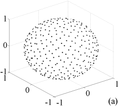
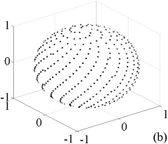
It should be noted that a more satisfactory sampling scheme in multi-D space can be generated by introducing different prime bases which connects to the Hammersley points based on Halton sequences [16].

II-B Multivariate empirical mode decomposition

The recent MEMD method has been shown its strength for VvS decomposition, especially for mode alignment problem and noise-assisted applications. The white noise decomposition test illustrates its remarkable dyadic filter bank property comparing to classic EMD and ensemble EMD [14]. The whole algorithm can be summarized in Algorithm 1.

Algorithm 1 : MEMD in 4-D space

• set $R_{1}(t)=F(t)$, $j=1$, and the values of $M$ and $b$; generate the projection direction set ${\mathcal{I}}_{b}^{M}$;

• extract $j$th IMF by sifting process $(F_{j}(t):={\mathcal{S}}^{N}[R_{j}](t))$

  • set intermediate curve $H_{j,0}(t)=R_{j}(t)$ and $n=0$;

  • approximate the local mean $T_{j,n}(t):={\mathcal{M}}[H_{j,n}](t)$;

    • for every direction $p_{m}\in{\mathcal{I}}_{b}^{M},m=0,1,\cdots,M-1$, project $H_{j,n}(t)$ into 1-D space, $h_{j,n}^{p_{m}}(t):={\mathcal{P}}_{p_{m}}[H_{j,n}](t)$;

    • detect all LELs of $h_{j,n}^{p_{m}}(t)$ (maximum location $t_{j,n,k^{+}}^{p_{m}}$ and minimum location $t_{j,n,k^{-}}^{p_{m}}$, $k^{+},k^{-}\in{\mathbb{N}}$) ;

    • generate upper $U_{j,n}^{p_{m}}(t)$ and lower $V_{j,n}^{p_{m}}(t)$ VvEs by interpolating data pairs $(H_{j,n}(t_{j,n,k^{+}}^{p_{m}}),t_{j,n,k^{+}}^{p_{m}})$ and $(H_{j,n}(t_{j,n,k^{-}}^{p_{m}}),t_{j,n,k^{-}}^{p_{m}})$ based on CSI;

    • set $T_{j,n}(t):=\frac{1}{2M}\sum_{m=0}^{M-1}U_{j,n}^{p_{m}}(t)+V_{j,n}^{p_{m}}(t)$;

  • update $H_{j,n+1}(t)=H_{j,n}(t)-T_{j,n}(t)$ and $n=n+1$;

  • calculate stopping criterion $\text{SD}_{j,n}$ as the one in [17];

  • repeat steps (B) to (E) until $\text{SD}_{j,n}\leq\text{SD}_{\text{Thr}}$, or the max iteration number $N$ is met; define $j$th IMF $F_{j}(t):=H_{j,n}(t)$;

• update $R_{j+1}(t)=R_{j}(t)-F_{j}(t)$, and $j=j+1$;

• repeat steps 2 to 3 until number of extrema in $R_{j}(t)$ is less than 2 or an expected IMF index is met, i.e., $j=J$.

In MEMD, the local mean approximation ${\mathcal{M}}[\cdot](t)$ could be considered as an ensemble approach, which means the idea mean curve $\hat{T}(t)$ may be exactly approximated as $M\rightarrow\infty$. In other words, we could re-define the local mean by $\hat{T}(t):={\mathcal{M}}[H](t):=\text{E}(\frac{1}{2}(U^{p_{m}}(t)+V^{p_{m}}(t))$, where E denotes the expectation over the direction $p_{m}$. In real application, the projection number $M$ needs not to be a large number compromising both computational complexity and approximation performance.

III Vector-valued empirical mode decomposition

In this section, a different EMD extension, namely the VEMD, will be explained, in which the VvEs of the given VvS are generated by back-projecting the 1-D envelopes interpolated in the projected space to the original 4-D space. Since the naive back-projection might result in infinite solutions, a novel optimization scheme will be designed to guarantee an unique VvE which should be also as smooth as possible.

III-A Optimization based back projection

Keeping the notation system in algorithm 1 but ignoring the trivial subindexes, in this subsection, $H(t),p_{m}$ denote the considering VvS and the projection direction, $U_{p_{m}}(t),V_{p_{m}}(t)$ denote the upper and lower VvEs w.r.t $p_{m}$ in the original 4-D space, and $u_{p_{m}}(t),v_{p_{m}}(t)$ denote the upper and lower envelopes w.r.t $p_{m}$ in the 1-D projected space.

Assuming $H(t)$ and $p_{m}$ are given, and the ${\mathcal{P}}_{p_{m}}[H](t)$ is the projected 1-D signal, the local maxima/minima of ${\mathcal{P}}_{p_{m}}[H](t)$ can be easily detected at the corresponding time locations $t_{k^{+}}$ and $t_{k^{-}}$, $k^{+},k^{-}\in{\mathbb{N}}$. With some interpolation method, e.g. the CSI, the 1-D upper $u_{p_{m}}(t)$ and lower $v_{p_{m}}(t)$ envelopes can be interpolated based on the pairs $({\mathcal{P}}_{p_{m}}[H](t_{k^{+}}),t_{k^{+}})$ and $({\mathcal{P}}_{p_{m}}[H](t_{k^{-}}),t_{k^{-}})$ separately. Now, we aim to project $u_{p_{m}}(t)$ and $v_{p_{m}}(t)$ back to the original 4-D space in order to obtain the VvEs $U_{p_{m}}(t):=(u_{p_{m}}^{[1]}(t),u_{p_{m}}^{[2]}(t),u_{p_{m}}^{[3]}(t))^{T}$ and $V(t):=(v_{p_{m}}^{[1]}(t),v_{p_{m}}^{[2]}(t),v_{p_{m}}^{[3]}(t))^{T}$ w.r.t the direction $p_{m}$.

Mathematically speaking, such back projection problem is equivalent to the solution problem of the linear system ${\mathcal{P}}_{p_{m}}[U_{p_{m}}](t)=u_{p_{m}}(t)$ (or ${\mathcal{P}}_{p_{m}}[V_{p_{m}}](t)=v_{p_{m}}(t)$), which has infinite solutions because the number of unknowns is larger than the number of equations. However, the infinite solutions can be constrained to unique one if next two properties can be maintained simultaneously: a) the back-projected VvEs $U_{p_{m}}(t)$ (or $V_{p_{m}}(t)$) should pass through the LELs $(H(t_{k^{+}}),t_{k^{+}})$ and $(H(t_{k^{-}}),t_{k^{-}})$ w.r.t direction $p_{m}$; b) the VvEs $U_{p_{m}}(t)$ (or $V_{p_{m}}(t)$) should be as smooth as possible. To investigate the smoothness of an unknown 4-D VvS $X(t):=(x^{[1]}(t),x^{[2]}(t),x^{[3]}(t))$, we may employ an $n$th order Sobolev norm funtional, i.e., the $L_{2}$ norm of the $n$th (weak) derivative of the function $X$

$$\leavevmode\resizebox{422.77661pt}{}{$\boldsymbol{S}^{(n)}[X]:=\|{\mathcal{D}}^{(n)}[x^{[1]}]\|_{L_{2}}^{2}+\|{\mathcal{D}}^{(n)}[x^{[2]}]\|_{L_{2}}^{2}+\|{\mathcal{D}}^{(n)}[x^{[3]}]\|_{L_{2}}^{2}$},$$ (6)

where ${\mathcal{D}}^{(n)}$ is the $n$th order derivative operator as its matrix form for discrete problem is well-known .

Now, the back-projected VvEs can be uniquely obtained by solving the following optimization problems

$$(P1)\quad\mbox{Minimize} \boldsymbol{S}^{(n)}[U_{p_{m}}](t)$$

  subject to $${\mathcal{P}}_{p_{m}}[U_{p_{m}}](t)=u_{p_{m}}(t)$$

$$U_{p_{m}}(t_{k^{+}})=H(t_{k^{+}}).$$

$$(P2)\quad\mbox{Minimize} \boldsymbol{S}^{(n)}[V_{p_{m}}](t)$$

  subject to $${\mathcal{P}}_{p_{m}}[V_{p_{m}}](t)=v_{p_{m}}(t)$$

$$V_{p_{m}}(t_{k^{-}})=H(t_{k^{-}})$$

In fact, (P1) and (P2) are both quadratic optimization problems with equality constraints. They can be written as quadratic optimization problems without constraints by solving the linear constraint system and then implementing the variable reduction.

III-B Vector-valued empirical mode decomposition

Comparing to the MEMD method in section II-B, the VEMD employs the back projection to obtain the VvEs from the envelopes interpolated in the 1-D projected space w.r.t a selected projection direction.

Most of the computation steps in VEMD algorithm are as the same as the ones in algorithm 1 except the step 2:(B):(c) which should be replaced by

Algorithm 2 : VEMD in 4-D space

• (B):(c) generate upper $u_{j,n}^{p_{m}}$ and lower $v_{j,n}^{p_{m}}(t)$ envelope in the 1-D projected space by interpolating data pairs $({\mathcal{P}}_{p_{m}}[H_{j,n}](t_{j,n,k^{+}}^{p_{m}}),t_{j,n,k^{+}}^{p_{m}})$ and $({\mathcal{P}}_{p_{m}}[H_{j,n}](t_{j,n,k^{-}}^{p_{m}}),t_{j,n,k^{-}}^{p_{m}})$ based on CSI; then solve the corresponding back projection optimization problem (P1) and (P2) to obtain the 4-D upper $U_{j,n}^{p_{m}}(t)$ and lower $V_{j,n}^{p_{m}}(t)$ envelopes;

It should be noted that in algorithm 2, the envelope interpolation in the 1-D projected space can be implemented by any reasonable interpolation method in order to meet different mathematical requirements, e.g. the method in [4].

IV Numerical studies

In this section, all the simulations are implemented in MATLAB on a laptop equipped with an i7-4700 quad-core CPU, 8 GB memory and under Windows. All optimization problems are solved by the standard CVX toolbox from [18]. To distinguish the associated variables in MEMD and VEMD, we employ the subscripts M and V.

In the VEMD, the order of the derivative operator in (6), the projection direction number and the prim base in (5) are free parameters, each of which may effect the behavior of the method. To determine each one, we study the decomposition problem of the following VvS

$$F(t) :=X(t)+Y(t),\;t\in[0,1],$$ (7)

$$X(t) :=\left(\begin{array}[]{c}x^{[1]}(t)\\ x^{[2]}(t)\\ x^{[3]}(t)\\ \end{array}\right)=\left(\begin{array}[]{c}(1+\cos(2\pi t))\sin(20\pi t)\\ (2+\cos(4\pi t))\sin(20\pi t)\\ (3+\cos(6\pi t))\sin(20\pi t)\\ \end{array}\right),$$

$$Y(t) :=\left(\begin{array}[]{c}y^{[1]}(t)\\ y^{[2]}(t)\\ y^{[3]}(t)\\ \end{array}\right)=\left(\begin{array}[]{c}\sin(4\pi t)\\ 2\sin(4\pi t)\\ 3\sin(4\pi t)\\ \end{array}\right).$$

Comparing to the signal model in (2), the components $X(t)$ and $Y(t)$ can be considered as the first IMF $F_{1}(t)$ and the residual $R_{2}(t)$, respectively. The reason that we set a common frequency of each $x^{[i]}(t)$ and $y^{[i]}(t)$ is to facilitate the discussion. Since the MEMD, as the same as the VEMD, has the mode alignment property (see [14]), different frequencies involved in the components $x^{[i]}(t)$ or $y^{[i]}(t)$ undoubtedly lead to many more decomposed IMFs, each of which should contain a particular frequency.

IV-A Derivative order

Selecting a unit projection direction $p=[\frac{1}{2},\frac{1}{2},\frac{\sqrt{2}}{2}]$, we can easily obtain the projected VvS ${\mathcal{P}}_{p}[F](t)$ together with its LELs $t_{k^{+}}/t_{k^{-}}$ (Fig.2 (d)). Based on these locations, by using a CSI, we can interpolate the envelopes $u_{p}(t),v_{p}(t)$ in the projected space (Fig.2 (d)), and the VvEs $U_{\text{M}}(t):=(u_{\text{M}}^{[1]}(t),u_{\text{M}}^{[2]}(t),u_{\text{M}}^{[3]}(t))^{T}$ and $V_{\text{M}}(t):=(v_{\text{M}}^{[1]}(t),v_{\text{M}}^{[2]}(t),v_{\text{M}}^{[3]}(t))^{T}$ in the original 4-D space (Fig.2 (a)-(c)). Fig.2 (e) illustrates that the projected VvEs $({\mathcal{P}}[U_{M}](t),{\mathcal{P}}[V_{M}](t))$ are nothing but the envelopes $(u_{p}(t),v_{p}(t))$ in the projected space. In other words, Fig.2 graphically explains why the MEMD interpolates the VvEs directly in the original space but not in the projected space.

Figure 2: The envelope interpolation in MEMD. (a)-(c) The VvS $F(t)$ and its interpolated VvEs $U_{\text{M}}(t)$ and $V_{\text{M}}(t)$ w.r.t an unit projection direction $p$; (d) The projected signal ${\mathcal{P}}_{p}[F](t)$ and its interpolated envelopes $u_{p}(t)$ and $v_{p}(t)$; (e) The absolute difference between the projected VvEs and the envelopes in the projected space, e.g. $\text{D}u_{\text{M}}(t):=|{\mathcal{P}}_{p}[U_{\text{M}}](t)-u_{p}(t)|$.

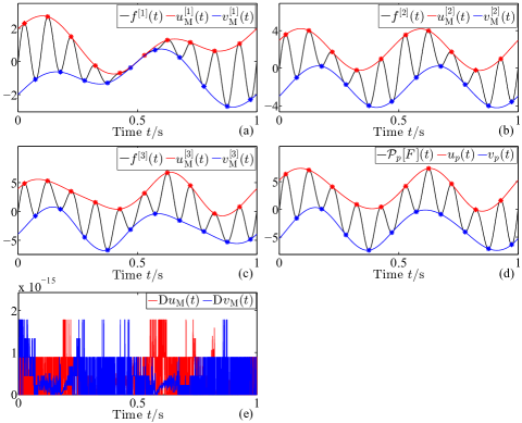
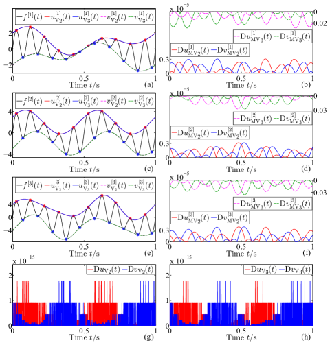
Now, based on the interpolated envelopes together with the LELs in the projected space, we can obtain the 4-D VvEs using the proposed back projection method, i.e. solving the optimization problems (P1) and (P2) described in Sec.III-A. Considering that, normally, the first order derivative won’t be an optimum choice for smoothness measurement [4], we set the 2nd or 3rd order derivative in (6) alternatively for simulation. Fig.3 presents the corresponding solved VvEs based on the data shown in Fig.2 (d).

In Fig.3, sub-figures (a)(c)(e) illustrate back-projected VvEs $U_{\text{V}_{2}}(t),V_{\text{V}_{2}}(t)$ and $U_{\text{V}_{3}}(t),V_{\text{V}_{3}}(t)$, where the subscripts $\text{V}_{2}$ and $\text{V}_{3}$ denote the 2nd and 3rd order derivative selected in VEMD each. To evaluate the interpolation performance, we take the VvEs interpolated in MEMD as a benchmark. Sub-figures (b)(d)(f) present the absolute differences between each VvE in VEMD and the corresponding VvE in MEMD, e.g. $\text{D}U_{\text{MV}_{2}}(t):=(\text{D}u_{\text{MV}_{2}}^{[1]}(t),\text{D}U_{\text{MV}_{2}}^{[2]}(t),\text{D}U_{\text{MV}_{2}}^{[3]}(t))^{T}:=|U_{\text{M}}(t)-U_{\text{V}_{2}}(t)|$. These figures imply that the VEMD with 2nd order derivative would be much close to the MEMD comparing to the VEMD with 3rd order derivative. This interesting phenomenon can be effortlessly understood if we can recall that the CSI requires the interpolated curve to be at most 2nd order continuously differentiable. Therefore, the VEMD with 2nd order derivative can produce similar results to the ones from MEMD, while the VEMD with 3rd order derivative can provide smoother interpolated curve. Finally, sub-figures (g)(h) imply both VvEs interpolated in VEMD satisfy the first equality constraint in (P1) and (P2) with high accuracy.

Figure 3: The envelope interpolation in VEMD. Left column (a)(c)(e): the VvS and its VvEs obtained by solving back projection problems (P1) and (P2) w.r.t an unit projection direction $p$. Subscripts $\text{V}_{2}$ and $\text{V}_{3}$ of the solution denote the 2nd and 3rd order derivative selected in (6) for VvE interpolation; Right column (b)(d)(f): absolute difference between interpolated VvEs in VEMD and the ones in MEMD shown in Fig.2, e.g. $\text{D}U_{\text{MV}_{2}}(t):=|U_{\text{M}}(t)-U_{\text{V}_{2}}(t)|$; Last row (g)(h): The absolute difference between the projected VvEs and the envelope in the projected space, e.g. $\text{D}u_{\text{V}_{2}}(t):=|{\mathcal{P}}_{p}[U_{\text{V}_{2}}](t)-u_{p}(t)|$.

IV-B Projection number and prime base

In section II-B we have shown that, given a fixed prime base for projection sampling, the local mean approximation operator ${\mathcal{M}}[\cdot]$ might be considered as an ensemble approach. In practice, we have to determine a finite projection number such that the approximation would be good enough or at least approximately convergent. Let’s consider again the VvS $F(t)$ in (7). If we apply the operator on $F(t)$ with a fixed projection number $M$, ${\mathcal{M}}^{M}[F](t)$ shall be the approximated local mean, e.g. ${\mathcal{M}}_{\text{M}}^{M}[F](t)$, the result of step (B) in the MEMD (algorithm 1), or the ${\mathcal{M}}_{\text{V}_{2}}^{M}[F](t)$ or ${\mathcal{M}}_{\text{V}_{3}}^{M}[F](t)$ in the VEMD (algorithm 2). To measure the approximation efficiency, we define a percent root mean squared difference (PRD) as an error function of the projection number $M$,

$$\text{PRD}(M):=\frac{\|{\mathcal{M}}^{M}[F](t)-Y(t)\|_{L_{2}}}{\|Y(t)\|_{L_{2}}}\times 100\%.$$ (8)

Fig.4 (a) describes the approximation performance of the operators ${\mathcal{M}}_{\text{M}}^{M}[\cdot]$, ${\mathcal{M}}_{\text{V}_{2}}^{M}[\cdot]$ and ${\mathcal{M}}_{\text{V}_{3}}^{M}[\cdot]$ for $b=2,M\in[5,1000]$. As can be seen, all PRD sequences decay dramatically in the beginning, and each one might be approximately convergent when $M\geq 256$. Since the sampled projection directions are not ideally uniform distributed on the sphere [15], the sampling error may result in slight oscillations on the PRD sequence. Therefore, we set $M=512$ for rest simulations.

Figure 4: Local mean approximation performance of operators ${\mathcal{M}}_{\text{M}}^{M}[\cdot]$, ${\mathcal{M}}_{\text{V}_{2}}^{M}[\cdot]$ and ${\mathcal{M}}_{\text{V}_{3}}^{M}[\cdot]$ in MEMD and VEMD. (a) PRD values of the three operators for $b=2$, and $M\in[5,1000]$; (b) PRD values of the three operators for $M=512$, and $b\in[2,80]$.

Fig.4 (b) presents the performance of all three approximation operators with different prime bases $b\in[2,80]$. It shows that different prime numbers do not effect the PRD values significantly. This is because the prime base only effects on the projection locations on the sphere (see Fig.1). When the projection number is large enough, approximation operator with different prime bases should provide consistent performance. In other words, the prime base can not be set as some number which is close to the projection number. Otherwise, from (3) and (4), we will find that $z_{b}(m)$ and $m$ may have strong correlation, e.g. partial linear dependence, that results in a non-uniform sampling on the sphere. Therefore, we set $b=2$ for rest simulations.

Fig.4 illustrates another exciting phenomenon: the approximation operator ${\mathcal{M}}_{\text{V}_{3}}^{M}[\cdot]$ works better than other two for arbitrarily selected projection number and prime base. This can be easily understood with following two considerations: 1) ${\mathcal{M}}_{\text{V}_{3}}^{M}[\cdot]$ requires higher order derivatives for smoothness evaluations than other two; 2) many common functions are continuously differentiable with high order. On the other hand, the performance of ${\mathcal{M}}_{\text{V}_{2}}^{M}[\cdot]$ and the one of ${\mathcal{M}}_{\text{M}}^{M}[\cdot]$ coincide each other perfectly, which further implies the effectiveness of the proposed method.

IV-C Decomposition performance

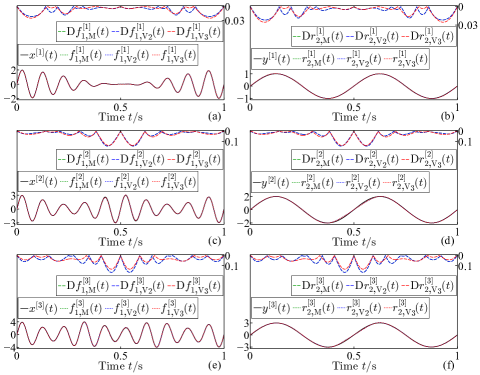
With the fixed parameters, the proposed VEMD can be applied to decompose the given VvS $F(t)$ in (7). The corresponding decomposition results are shown in Fig.5. As can be seen, all decomposed components by using MEMD or VEMD with different derivative orders are very similar to the ideal ones. To numerically distinguish the decomposition performance, the PRDs of the decomposition results w.r.t each method are listed in Table-I. The numerical results support our observation again: the VEMD with 3rd derivative order is better than the one with 2nd derivative order and the MEMD; and the latter two methods have similar behavior from mathematic point of view.

Figure 5: Decomposition results of the given VvS $F(t)$ in (7) by using MEMD and VEMD methods. Left column (a)(c)(e): the original component $X(t)$, the first decomposed Imfs using MEMD ($F_{1,\text{M}}(t)$), and VEMD with 2nd derivative ($F_{1,\text{V}_{2}}(t)$) and 3rd derivative ($F_{1,\text{V}_{3}}(t)$), and the absolute difference between $X(t)$ and each $F_{1,\cdot}(t)$, e.g. $\text{D}F_{1,\text{M}}(t):=|X(t)-F_{1,\text{M}}(t)|$; Right column (b)(d)(f): the original component $Y(t)$, the residual $R_{2,\text{M}}(t)$, $R_{2,\text{V}_{2}}(t)$ and $R_{2,\text{V}_{3}}(t)$, and the corresponding absolute difference.

TABLE I: PRD of the decomposition results using MEMD and VEMD

PRD(%)	M	$\text{V}_{2}$	$\text{V}_{3}$
$F_{1,\cdot}(t)$	2.95	2.95	2.65
$R_{2,\cdot}(t)$	3.10	3.10	2.79

V Conclusion

As a representative data-driven method, EMD can provide finer time-frequency analysis of any nonlinear and/or nonstationary signal sampled in (non-)uniform grids. This paper introduced a novel method to extend the classical EMD for vector-valued signal decomposition. Different from the existing MEMD, our proposed VEMD obtains the local mean curve by projecting the envelopes obtained in 1-D projected space back into the original multi-D space. Since the VEMD does not require any particular envelope interpolation method, it is more general and flexible compared to the MEMD for many potential applications. In addition, with the method introduced in [19], we can generate a time-frequency representation of any VvS which can then provide meaningful information for further vector-valued data analysis.

References

- [1] N.E. Huang, Z. Shen, S.R. Long, M.C. Wu, H.H. Shih, Q. Zhang, N.-C. Yen, C.C. Tung and H.H. Liu, The empirical mode decomposition and the Hilbert spectrum for nonlinear and non-stationary time series analysis, Proc. R. Soc. London A, vol. 454, pp. 903-995, 1998.
- [2] N.E. Huang, and S.S.P. Shen, Hilbert-Huang transform and its applications, World Scientific Publishing, Singapore, 2005.
- [3] T.Y. Hou, and Z. Shi, Adaptive data analysis via sparse time-frequency representation, Adv. Adapt. Data Anal., vol. 3, pp. 1-28, 2011.
- [4] B. Huang, and A. Kunoth, An optimization-based empirical mode decomposition scheme, J. Comp. Appl. Math., vol. 240, pp. 174-183, 2013.
- [5] N.E. Huang, Z. Wu, S.R. Long, K.C. Arnold, X. Chen, and K. Blank, On instantaneous frequency, Adv. Adapt. Data Anal., vol. 1, pp. 177-229, 2009.
- [6] J. Rudi, R. Pabel, G. Jager, R. Koch, A. Kunoth, and H. Bogena, Multiscale analysis of hydrologic time series data using the Hilbert-Huang-Transform (HHT), Vadose Zone J., vol. 9, pp. 925-942, 2010.
- [7] N.E. Huang, Z. Wu, A review on Hilbert-Huang transform: Method and its applications to geophysical studies, Rev. Geohpys., vol. 46, pp. 1-23, 2008
- [8] G. Jager, R. Koch, A. Kunoth, and R. Pabel, Fast empirical mode decompositions of multivariate data based on adaptive spline-wavelets and a generalization of the Hilbert-Huang-Transform (HHT) to arbitrary space dimensions, Adv. Adapt. Data Anal., vol. 2, pp. 337-358, 2010.
- [9] T. Tanaka, and D.P. Mandic, Complex empirical mode decomposition, IEEE Signal Process. Lett., vol. 14, pp. 101-104, 2007.
- [10] G. Rilling, P. Flandrin, P. Gonçalves, and J.M. Lilly, Bivariate empirical mode decomposition, IEEE Signal Process. Lett., vol. 14, pp. 936-939, 2007.
- [11] N.U. Rehman, and D.P. Mandic, Multivariate empirical mode decomposition, Proc. Roy. Soc. London A, vol. 466, pp. 1291-1302, 2010.
- [12] N.U. Rehman, and D.P. Mandic, Empirical mode decomposition for trivariate signals, IEEE Trans. Signal Process., vol. 58, pp. 1059-1068, 2010.
- [13] N.U. Rehman, and D.P. Mandic, Filterbank property of multivariate EMD, IEEE Trans. Signal Process., vol. 59, pp. 2421-2426, 2011.
- [14] D.P. Mandic, N.U. Rehman, Z. Wu, and N.E. Huang, Empirical mode decomposition-based time-frequency analysis of multivariate signals, IEEE Signal Process. Magazine, vol. 30, pp. 74-86, 2013.
- [15] J. Cui, and W. Freeden, Equidistribution on the sphere, SIAM J. Sci. Comput., vol. 18, pp. 595-609, 1997.
- [16] H. Niederreiter, Random number generation and quasi-Monte Carlo methods, Chapter 3, Society for Industrial and Applied Mathematics, Philadelphia, USA, 1992.
- [17] G. Rilling, P. Flandrin, and P. Gonçalves, On empirical mode decomposition and its algorithms, Proc. IEEE-EURASIP Workshop Nonlinear Signal Image Process. NSIP-03, Grado, Italy, 2003.
- [18] M. Grant, and S. Boyd, CVX Users Guide, available online: http://cvxr.com, 2011.
- [19] B. Huang, and A. Kunoth, A unique polar representation of the hyperanalytic signal, IEEE Int. Conf. on Acoustics, Speech, and Signal Processing (ICASSP), pp. 379-383, Florence, Italy, May 2014.