The galaxy - dark matter halo connection: which galaxy properties are correlated with the host halo mass?

Abstract

We demonstrate how the properties of a galaxy depend on the mass of its host dark matter subhalo, using two independent models of galaxy formation. For the cases of stellar mass and black hole mass, the median property value displays a monotonic dependence on subhalo mass. The slope of the relation changes for subhalo masses for which heating by active galactic nuclei becomes important. The median property values are predicted to be remarkably similar for central and satellite galaxies. The two models predict considerable scatter around the median property value, though the size of the scatter is model dependent. There is only modest evolution with redshift in the median galaxy property at a fixed subhalo mass. Properties such as cold gas mass and star formation rate, however, are predicted to have a complex dependence on subhalo mass. In these cases subhalo mass is not a good indicator of the value of the galaxy property. We illustrate how the predictions in the galaxy property - subhalo mass plane differ from the assumptions made in some empirical models of galaxy clustering by reconstructing the model output using a basic subhalo abundance matching scheme. In its simplest form, abundance matching generally does not reproduce the clustering predicted by the models, typically resulting in an overprediction of the clustering signal. Using the predictions of the galaxy formation model for the correlations between pairs of galaxy properties, the basic abundance matching scheme can be extended to reproduce the model predictions more faithfully for a wider range of galaxy properties. Our results have implications for the analysis of galaxy clustering, particularly for low abundance samples.

1 Introduction

How well do different galaxy properties correlate with halo mass? Given the value of a galaxy property, such as its stellar mass or cold gas mass, how good an indicator is this of the mass of the galaxy’s dark matter halo? If we know the mass of a dark matter halo in a N-body simulation, is there a clear indication of what the properties of a galaxy hosted by the halo should be? Here we use two independent models of galaxy formation to answer these questions. Our results have implications for empirical models which aim to describe measurements of galaxy clustering and the construction of galaxy catalogues from N-body simulations of structure formation.

The idea that there should be a connection between the properties of a galaxy and the mass of its host dark matter halo lies at the core of galaxy formation theory. White & Rees (1978) were the first to propose that galaxies form when baryons condense inside the gravitational potential wells of dark matter halos. The radiative cooling of hot gas is just one of the many processes believed to be relevant for galaxy evolution (for reviews see Baugh 2006 and Benson 2010). Even though 35 years that have elapsed since the framework for hierarchical galaxy formation was laid down, many of the key processes remain poorly understood. Current models use a combination of direct simulation and so called “sub-grid” modelling to follow the formation and evolution of galaxies (e.g. Cole et al. 2000; Springel et al. 2005; Crain et al. 2009; Schaye et al. 2010; Guo et al. 2011; Vogelsberger et al. 2014; Schaye & et al. 2014). These models now give encouraging reproductions of some of the basic characteristics of the observed population of galaxies.

Given the basic tenet laid down by White & Rees (1978) it is natural that there should be some connection between the mass of a dark matter halo and the properties of the galaxy inside it, with the biggest galaxies expected to reside in the biggest halos since these halos contain the most baryons. This scaling is shaped by feedback processes which regulate the rate of star formation. The efficiency of galaxy formation varies with halo mass, reaching a peak in halos around the mass of that which hosts the Milky Way (Eke et al. 2005; Guo et al. 2010). In low mass halos, heating of the intergalactic medium by photo-ionizing photons and of the interstellar medium by supernovae stymie the build up of stellar mass (Benson et al. 2002; Somerville 2002). In high mass halos, modellers have appealed to the injection of energy into the hot halo by active galactic nuclei (AGN) to reduce the predicted abundance of massive galaxies (Benson et al. 2003; Bower et al. 2006; Cattaneo et al. 2006; Croton et al. 2006; Lagos, Cora & Padilla 2008).

Whilst there is a relation between halo mass and galaxy property for some properties, as we will demonstrate, this does not imply that all the properties of a galaxy can be deduced once the mass of the host halo is specified. Also, the relative importance of the processes which take part in galaxy formation varies both with halo mass and redshift. This in turn could lead to changes in the manner in which galaxy properties scale with halo mass and introduce scatter through a dependence on halo formation histories.

Observed scaling relations between galaxy properties also suggest a connection between halo mass and galaxy luminosity (see Tasitsiomi et al. 2004; Dutton et al. 2010; Trujillo-Gomez et al. 2011a). Tully & Fisher (1977) found a tight correlation between galaxy luminosity, $L$, and the circular velocity of the disk, $V_{\rm c}$, for spiral galaxies. In the optical, the scaling is $L\propto V_{\rm c}^{3}$ (Mocz et al. 2012). In the near-infrared this becomes $L\propto V_{\rm c}^{4}$ (Verheijen 1997; Tully et al. 1998). A similar scaling exists for elliptical galaxies, albeit with a larger scatter (Faber & Jackson 1976).

It is tempting to use these observed galaxy scaling relations to assign a luminosity to a dark matter structure with a given circular velocity. However, there are number of problems with such an approach. First, the precise scaling relation depends on the galaxy selection, with different scalings found for spirals and ellipticals. Second, the observed relations only cover a limited dynamic range in circular velocity and luminosity, and so cannot be applied to low mass halos. Finally, the application of the scaling relation assumes that the circular velocity measured for the galaxy can easily be related to the circular velocity which characterizes the dark matter halo, whereas in reality these are measured at very different radii. Models suggest that shifts of 20-30% are common between the circular velocity at the half-light radius of the galaxy and that obtained at the virial radius of the halo (e.g. Cole et al. 2000). This difference in velocity would make a big difference to the assigned galaxy luminosity, given the steep dependence of the observed scaling relations on circular velocity.

A more promising approach to connect galaxies with their host dark matter halos is the sub-halo abundance matching (SHAM) technique introduced by Vale & Ostriker (2004), who proposed a monotonic relation between galaxy luminosity and halo mass with zero scatter (e.g. Kravtsov, Gnedin & Klypin 2004; Vale & Ostriker 2006; Conroy, Wechsler & Kravtsov 2006; for a review of galaxy clustering models see Baugh 2013). A galaxy catalogue with spatial information can be constructed using SHAM by taking a sample of galaxy luminosities, generated, for example, using an observed galaxy luminosity function, sorting in luminosity and then matching up this list of galaxies with a sorted list of subhalo masses obtained from an N-body simulation. The SHAM technique has been used extensively to model galaxy clustering (eg. Conroy, Wechsler & Kravtsov 2006; Shankar et al. 2006; Baldry, Glazebrook & Driver 2008; Moster et al. 2010; Guo et al. 2010; Behroozi, Conroy & Wechsler 2010; Wake et al. 2011; Hearin & Watson 2013; Nuza et al. 2013; Reddick et al. 2013; Simha & Cole 2013).

The modern implementation of SHAM has one important difference from the original proposal of Vale & Ostriker (2004). This regards the treatment of satellite galaxies. These galaxies reside in dark matter structures called subhalos which may have experienced significant mass loss, depending on their orbit within their more massive dark matter halo. Using the instantaneous subhalo mass measured from a N-body simulation would therefore lead to an error in the assigned luminosity. To circumvent this, the mass of the subhalo at the point of infall to the larger structure is commonly used (Conroy, Wechsler & Kravtsov 2006; Vale & Ostriker 2006). We note that recent N-body simulations have shown that the maximum halo mass is attained prior to infall, with some mass loss already occuring before the halo crosses the virial radius of the more massive halo (Behroozi et al. 2014). Furthermore, some satellite galaxies should be assigned to subhalos which can no longer be identified in a given simulation output due to the finite resolution. The issue of identifying a suitable dark matter structure to assign a galaxy to can be avoided if multiple outputs are available and the formation history of subhalos can be extracted (Conroy, Wechsler & Kravtsov 2006; Conroy & Wechsler 2009; see also Klypin et al. 2013 and Guo & White 2014 for requirements on the resolution of subhalos).

The original SHAM proposal relies on two key assumptions: (i) there is zero scatter between the galaxy property and halo mass, (ii) the impact of environmental effects on galaxy properties can be ignored. We will show that the first assumption is not supported by current galaxy formation models. The second assumption is also not held in most galaxy formation models, which explicitly treat gas cooling onto satellites and centrals differently (but see Font et al. 2008 and Guo et al. 2011 for alternative models). Hydrodynamic simulations show that this distinction may be blurred, with gas cooling continuing onto satellite galaxies (McCarthy et al. 2008; Simha et al. 2009). Observationally, the environment is found to shape the properties of galaxies (Balogh et al. 2004; Peng et al. 2010).

Even though the basic SHAM model is still discussed extensively in the literature (e.g. to give just two recent examples Finkelstein et al. (2015); Yamamoto, Masaki & Hikage (2015)), we note that various extensions to the model have been proposed which try to account for scatter in the value of a galaxy property associated with a given subhalo mass (Tasitsiomi et al. 2004; Behroozi, Conroy & Wechsler 2010; Moster et al. 2010; Neistein et al. 2011; Reddick et al. 2013) and which assign galaxy properties that do not have a simple dependence on halo mass (Rodríguez-Puebla et al. 2011; Hearin & Watson 2013; Gerke et al. 2013; Masaki, Lin & Yoshida 2013; Kravtsov, Vikhlinin & Meshscheryakov 2014; Hearin et al. 2014; Rodriguez-Puebla et al. 2014).

Here we examine the nature of the galaxy - halo connection using semi-analytic galaxy formation models (SAMs). These models represent a physically motivated, ab-initio calculation which tracks the fate of the baryonic content of the Universe. SAMs naturally predict the number and properties of galaxies in dark matter halos as a function of halo mass. Simha et al. (2012) carried out a similar analysis using smoothed particle hydrodynamics simulations. These simulations were run using small computational volumes and so did not include AGN feedback, which meant that the high mass end of the stellar mass - halo mass relation could not be studied. One advantage of using SAMs is that they can be run using the dark matter halo merger trees from N-body simulations covering different volumes and mass resolutions, allowing a very wide dynamic range of mass to be probed at a low computational cost. To establish the robustness of the model predictions, we use two SAMs from independent groups: one which uses GALFORM (Lagos et al. 2012) and the other which uses the L-GALAXIES code (Guo et al. 2011). These models are representative of the current state-of-the-art of semi-analytical modelling.

The main aim of our paper is to establish which galaxy properties show a simple dependence on subhalo mass and how much scatter there is in the value of a galaxy property for a given halo mass. We consider the intrinsic galaxy properties of stellar mass, cold gas mass, star formation rate and black hole mass. We also study luminosities at different wavelengths, ranging from the ultra-violet, which is sensitive to the recent star formation history of a galaxy, to the near-infrared, which correlates more closely with its stellar mass. To illustrate the features of the model predictions, we compare the output of the galaxy formation model to some simple empirical models of galaxy clustering. We do this by applying the original, baisc SHAM model to reconstruct the SAM catalogues, comparing the clustering measured from the reconstructed catalogue with the prediction from the original catalogue. Taking advantage of the galaxy formation output, which tells us how different galaxy properties are correlated, we also consider a simple “two-step” SHAM approach for properties which do not meet the SHAM hypothesis themselves (see e.g. Rodríguez-Puebla et al. 2011). This also allows us to include at some level the scatter in the galaxy property - subhalo mass relation (see Trujillo-Gomez et al. 2011b; Hearin & Watson 2013; Masaki, Lin & Yoshida 2013 for more detailed discussion of models with similar aims). A key advantage of our study is that we extract the subhalo mass at infall into a more massive halo using the halo merger trees which are used in the semi-analytical model. This means that the problem of “missing subhalos” that afflicts SHAM when applied to a single N-body output is not an issue.

Our earlier paper comparing the clustering predictions made by different SAMs shows that the models are sufficiently robust for the exercise carried out here (Contreras et al. 2013). For galaxy samples selected by stellar mass, the L-GALAXIES and GALFORM models make remarkably similar clustering predictions on large scales. There are differences in the clustering predicted on small scales, but Contreras et al. (2013) show how these can be understood in terms of choices made in the implementation of galaxy mergers (see Section 2.4 for further discussion).

The layout of the paper is as follows. In Section 2 we first introduce the two semi-analytical models of galaxy formation used (§ 2.1) and the N-body simulations they are implemented in (§ 2.2). The definition and identification of subhalos is discussed in § 2.3; subhalos also play a role in galaxy mergers, as set out in § 2.4. The resolution ranges of the predictions, in terms of subhalo mass and galaxy properties is covered in § 3. The main results are presented in § 4, where we present model predictions for how galaxy properties depend on subhalo mass (§ 4.1), show which halos contribute to galaxy samples when different selections are applied (§ 4.2) and illustrate what happens when SHAM is used to reconstruct the theoretical models (§ 4.3). Our results are summarized and presented along with our conclusions in § 5.

2 The galaxy formation models

Here we give a brief overview of the galaxy formation models used in our study along with the specifications of the N-body simulations they are grafted onto. In Section 2.1 we briefly introduce the two SAMs and list the physical process they attempt to model. In Section 2.2 we describe the dark matter simulations in which both SAMs are implemented. The definitions of subhalo mass used in the two models is discussed in Section 2.3. Finally, in Section 2.4 we list the steps necessary to be able to compare models which employ different definitions of subhalo mass.

2.1 Semi-analytic models

The SAMs used in our comparison are those of Lagos et al. (2012) (hereafter L12) and Guo et al. (2011) (henceforth G11) .

The objective of SAMs is to model the main physical processes involved in galaxy formation and evolution in a cosmological context: (i) the collapse and merging of dark matter halos; (ii) the shock heating and radiative cooling of gas inside dark matter halos, leading to the formation of galaxy discs; (iii) quiescent star formation in galaxy discs; (iv) feedback from supernovae (SNe), from accretion of mass onto supermassive black holes and from photoionization heating of the intergalactic medium (IGM); (v) chemical enrichment of the stars and gas; (vi) dynamically unstable discs; (vii) galaxy mergers driven by dynamical friction within dark matter halos, leading to the formation of stellar spheroids, which may also trigger bursts of star formation. The two models have different implementations of each of these processes. By comparing models from different groups we can get a feel for which predictions are robust and which depend on the particular implementation of the physics.

The G11 model is based on various models from the Munich group (De Lucia, Kauffmann & White 2004; Croton et al. 2006; De Lucia & Blaizot 2007). The L12 model is a development of the model of Bower et al. (2006) which includes AGN heating of the cooling gas in massive halos. The L12 model has an improved treatment of star formation, breaking the interstellar medium into molecular and atomic hydrogen components (Lagos et al. 2011). One important difference between G11 and L12 is the implementation of cooling in satellite galaxies. In L12, a galaxy is assumed to lose its hot gas halo completely once it becomes a satellite; in G11, this process is more gradual and depends on the orbit of the satellite. Another important difference is the treatment of galaxy mergers. This will be discussed in Section 2.4 after we have introduced the N-body simulations used and the dark matter halo catalogues derived from them.

Simulation	$N_{\rm P}$	$m_{\rm P}/h^{-1}{\rm M_{\odot}}$	$L/h^{-1}{\rm Mpc}$
MS-I	$2160^{3}$	$8.61\times 10^{8}$	500
MS-II	$2160^{3}$	$6.88\times 10^{6}$	100

Table 1: The numerical parameters of the N-body simulations used. MS-I is the N-body simulation of Springel et al. (2005) and MS-II is the simulation described by Boylan-Kolchin et al. (2009).

2.2 N-body simulations

The SAMs used in this paper are both implemented in two N-body simulations, the Millennium I simulation (Springel et al. 2005, hereafter MS-I) and the Millennium II simulation (Boylan-Kolchin et al. 2009, MS-II from now on). The properties of the simulations are listed in Table 1. These two simulations have the same cosmology and the same number of particles, but employ different volumes and hence have different mass resolutions. There are 63 and 67 simulation outputs between $z=127$ and $z=0$ for MS-I and MS-II respectively. Halo finding algorithms were run on these outputs and used to build halo merger trees, as outlined in the next section. These trees are the starting point for the SAMs. By implementing the SAMs in different volume simulations, we can study the model predictions over a much wider range of halo mass than would be possible with a single simulation.

2.3 Dark matter subhalos

Once a halo becomes part of a more massive structure it is called a subhalo. The subhalo can retain its identity for some time after becoming gravitationally bound to the larger halo. Tidal forces lead to the removal of mass from the subhalo. The extent of this mass “stripping” depends upon the orbit followed by the satellite, with the tidal forces being stronger closer to the centre of the main halo. Dynamical friction will also cause the orbit of the subhalo to decay, moving the subhalo closer to the centre of the halo.

Friends-of-Friends (FoF) groups (Davis et al. 1985) are identified in each simulation output and retained down to 20 particles. SUBFIND is run on these groups to identify subhalos within the FoF groups (Springel et al. 2001). The construction of the dark matter halo merger histories using this information differs from this point onwards between the two groups (for further details of the merger tree construction, see Guo et al. 2011 and Jiang et al. 2014).

Eventually, if the mass-stripping is severe, SUBFIND will no longer be able to locate the subhalo. This poses a problem when attempting to apply SHAM to a single output from a N-body simulation. If many outputs are available, however, it is possible to build halo merger trees and to track the subhalo until SUBFIND is unable to locate it; thereafter the location of the galaxy associated with the subhalo is typically assigned to the potential minimum of its subhalo (Jiang et al. 2014).

As a result of the mass stripping experienced by subhalos, neither the instantaneous mass nor the maximum effective circular velocity of the halo rotation curves are useful indicators of the subhalo mass prior to infall (Ghigna et al. 1998; Kravtsov, Gnedin & Klypin 2004). Conroy, Wechsler & Kravtsov (2006) proposed that the mass of the subhalo at infall should be used instead as a more reliable measure of the subhalo mass, using the effective maximum circular velocity as a proxy (see also Vale & Ostriker 2006).

Here, we use the mass of the subhalo at the point of infall into a larger structure as obtained from the halo merger history if the host galaxy is a satellite, or the current halo mass if the galaxy is a central. Throughout the paper we will refer to the subhalo mass at infall as the subhalo mass unless explicitly stated otherwise.

The subhalo mass is obtained from the halo merger history, which is constructed using independent algorithms by the Durham and Munich groups. G11 construct dark matter halo merger trees by first running a FoF percolation algorithm on each simulation output or snapshot. SUBFIND is then run on the FoF halos to identify the bound particles and substructures within the halo. The merger tree is constructed by linking a subhalo in one output to a unique descendant subhalo in the subsequent snapshot. The halo merger tree used in the Munich SAM is therefore a subhalo merger tree. The L12 SAM uses the DHalos merger tree construction (Jiang et al. 2014; see also Merson et al. 2013 and Gonzalez-Perez et al. 2014). The initial steps are the same as in the Munich case, running FoF and SUBFIND on the simulation outputs. Additional considerations are applied in the construction of the DHalo merger trees. These include the requirement of the Durham SAM that halo mass increases monotonically with the age of the universe and the analysis of the halo at future snapshots to avoid the premature linking of halos which pass through another halo. The relation between subhalo masses in the L-GALAXIES and GALFORM cases is composed of an offset in mass and a scatter (Jiang et al. 2014). In §3.1 we will come up with a simple scheme to relate halo masses in the two SAMs.

2.4 Galaxy mergers

SAMs generally distinguish between two classes of satellite galaxies, type-I satellites which are associated with resolved DM subhalos and type-II satellites, also called “orphans”, for which the host subhalo can no longer be identified by SUBFIND. In L-GALAXIES, this information is used to decide which galaxies are candidates to merge with the central galaxy in the halo. Satellite galaxies which are associated with a resolved subhalo, i.e. type-I galaxies, are not allowed to merge with the central galaxy in their host dark matter halo. Once sufficient stripping of the dark matter has occured, such that the host subhalo can no longer be resolved and the type-I galaxy has become a type-II, a dynamical friction timescale is calculated for the galaxy to merge with the central. In the GALFORM model studied here, the presence of the subhalo is ignored for this purpose and all satellite galaxies are considered as candidates to merge with the central galaxy and a dynamical friction timescale is calculated for each satellite. This choice leads to a difference in the small-scale clustering predicted by the L-GALAXIES and GALFORM models, even in the case when the models contain the same number of satellites, as the radial distribution of satellites is different (Contreras et al. 2013). We note that in the current version of GALFORM it is possible to select a galaxy merger scheme that operates in the same fashion as the one used in L-GALAXIES (Campbell et al. 2014).

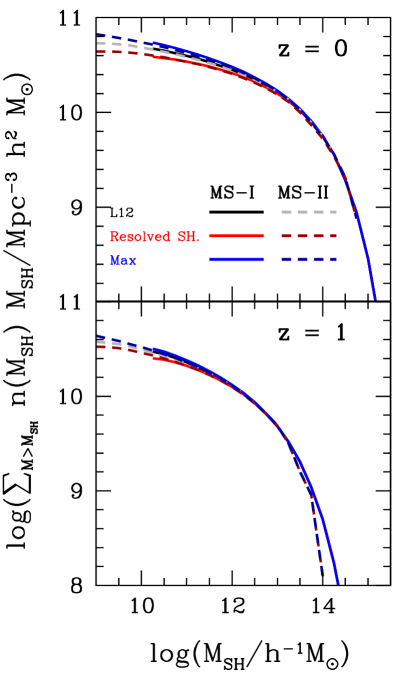
Figure 1: The cumulative mass contained in subhalos in the L12 model at $z=0$ (top) and $z=1$ (bottom). The solid lines show predictions from the MS-I and the dashed lines from MS-II. The black curves show the predictions using both resolved and unresolved subhalos (as obtained from the halo merger tree; see text). The red curves show the results for resolved subhalos only. The blue curves show the predictions for a model in which the number of subhalos is maximized by, effectively, allowing all halos to cool gas efficiently by removing stellar and photoionization feedback and switching off galaxy mergers.

3 Resolution limits of the SAMs

In this section we explain how we determine the range of subhalo masses and galaxy properties over which we consider the results obtained from the MS-I and MS-II simulations. Section §3.1 discusses the subhalo mass function and §3.2 presents the limits for the different galaxy properties.

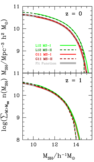
Figure 2: The distribution of subhalo masses in the L12 and G11 models, using the MS-I (solid lines) and MS-II (dashed lines), as labelled in the top panel, at $z=0$ (top) and $z=1$ (bottom). The thick grey line shows a fitting function which matches the subhalo mass function in the G11 model from MS-I for subhalos more massive than $10^{11}h^{-1}{\rm M_{\odot}}$ and from the MS-II for less massive halos. From now on, the subhalo masses quoted for both SAMs will be rescaled with reference to this curve, such that the predicted subhalo mass functions coincide with the fitting function.

3.1 The subhalo mass function

The cumulative distribution of subhalos masses in the L12 model is shown in Fig. 1, in which we plot the total mass contained in subhalos with masses greater than $M_{\rm sh}$, $\int_{M_{\rm sh}}^{\infty}n_{sh}(M)M{\rm d}M$, at $z=0$ (top) and $z=1$ (bottom). Due to the way in which we construct the subhalo mass function by using galaxies to point to their host subhalo, the subhalo mass function is nominally dependent on the galaxy formation model used. In the case of central galaxies, the mass of the host halo is used. For satellite galaxies we always use the mass of the host halo at the time of infall into a more massive structure. This information is obtained from the galaxy merger history predicted by the SAM.

The number of galaxies output by the SAM can change if, for example, the heating of the intergalactic medium by photoionization varies or the rate at which galaxies merge is altered. To explore the dependence of the subhalo mass function on galaxy formation physics, we have run an extreme variant of the L12 model in which we have deliberately set out to maximize the number of galaxies and, consequently, the number of subhalos picked up from the dark matter halo merger trees. This model has a cooling time set to zero in all halos, has no supernova feedback and has a galaxy merger timescale that is set to infinity. This means that galaxies will form in all subhalos and will not be removed by mergers. The mass in subhalos in this variant model is shown by the blue curves in Fig. 1. The agreement with the predictions using the standard L12 model is impressive; the subhalo mass functions are indistinguishable at $z=0$ above a subhalo mass of $10^{12}h^{-1}{\rm M_{\odot}}$, and only differ by up to around 50% at lower masses.

The results from the MS-I and MS-II simulations overlap reasonably well, with the MS-II predictions extending to lower subhalo masses and displaying more noise at the high-mass end due to the smaller simulation volume. The black line in Fig. 1 shows the mass in subhalos associated with all galaxies (i.e. for type-II galaxies without a resolved subhalo, we use the subhalo mass at infall), whereas the red curve shows how this mass is reduced when only galaxies attached to resolved subhalos are considered.

We now compare in Fig. 2 the subhalo mass functions obtained from the L12 and G11 SAMs. One difference between the subhalo masses reported by the two groups is that the DHalo mass used in GALFORM corresponds to an integer number of particles whereas a virial mass is calculated in L-GALAXIES. Hence, the G11 subhalo masses can extend down to lower masses than in the L12 case. The G11 subhalo masses can also decrease over time, unlike the DHalo masses, which, by construction, increase monotonically.

To enable us to plot galaxy properties against subhalo mass and to compare the two models using the MS-I and MS-II simulations, we need to take into account the offset in the predicted subhalo mass functions, as plotted in Fig. 2, which is due to the differences mentioned above in the definition of halo mass. We do this by defining a smooth function which describes the form of the subhalo mass function. We force this function to fit the subhalo mass function of the G11 model using the MS-I for masses above $10^{11}h^{-1}{\rm M_{\odot}}$. For halos less massive than this value, we use the G11 subhalo mass function from MS-II. The L12 subhalo masses are effectively rescaled, so that for a given subhalo abundance, the subhalo mass is that derived from the smooth fitting function at the same space density of objects.

The original subhalo mass functions of L12 and G11 run with MS-I and MS-II are shown in Fig. 2 for $z=0$ and $z=1$. The differences in the subhalo mass functions in the two models are clearly visible and depend on redshift. The smooth fitting function derived from the combination of G11 run with the MS-I and MS-II is shown as a thick grey line. From now on, all the SAM predictions will use this subhalo mass definition.

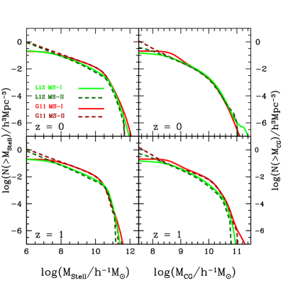
Figure 3: Cumulative stellar mass (left panels) and cold gas mass (right panels) functions for $z=0$ (top) and $z=1$ (bottom), for the L12 and G11 models, as labelled, obtained from the MS-I (solid lines) and MS-II (dashed lines).

3.2 Galaxy properties

The distributions of galaxy properties predicted by the models are more complex than those of subhalos. One issue is that for some properties, such as black hole mass or star formation rate, some galaxies are predicted to have zero values. The fraction of galaxies with zero values for a particular property can vary strongly between models. Hence, we do not attempt to replicate the approach taken for subhalo masses in the previous section. Instead we determine the range of property values to use from the MS-I and MS-II runs for each model separately.

The distribution of cold gas masses and stellar masses predicted by the SAMs is plotted in Fig. 3. Whilst there is, reassuringly, reasonable agreement between the predictions of a given model for the MS-I and MS-II runs for intermediate property values, there are clear differences between the L12 and G11 models. This is to be expected given the differences in the way in which the model parameters are calibrated and in choices such as the stellar initial mass function and the stellar population synthesis model used to convert the predicted star formation histories into luminosities.

We use the galaxy properties predicted using the MS-I run for galaxies with larger values of properties such as stellar mass or cold gas mass. Moving in the direction of smaller property values, once the cumulative distribution obtained from MS-I differs from that recovered using MS-II by more than a given amount, we switch to using the higher mass resolution MS-I results. Where practicable, we set the tolerance between the mass functions to be 5% before switching over to the MS-II predictions. Combined with the overall differences between the model predictions, this means that the transition between the MS-I and MS-II predictions is made at different property values for each model. To compare models, we set a number density to define galaxy samples, and select property values in each model to attain this number density.

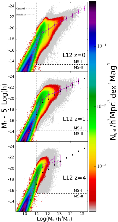
Figure 4: The distribution of the rest-frame $r$-band magnitude as a function of subhalo mass predicted in the L12 model, at $z=0$ (top), $z=1$ (middle) and $z=4$ (bottom). The colour shading represents the space density of galaxies as indicated by the colour bar on the right. The symbols with error bars show the median $r$-band magnitude and the 20-80^th percentile range for all galaxies. The black dots in the $z=1$ and $z=4$ panels show the median of the $r$-band magnitude at $z=0$, which is reproduced in these panels for reference. Different line styles show the median relation for centrals (dashed lines) and satellites (dotted lines) separately. The dashed line box separates the MS-I predictions (top right region) from those obtained from the MS-II, where the cumulative luminosity functions from the MS-I and MS-II differ by more than 5%.

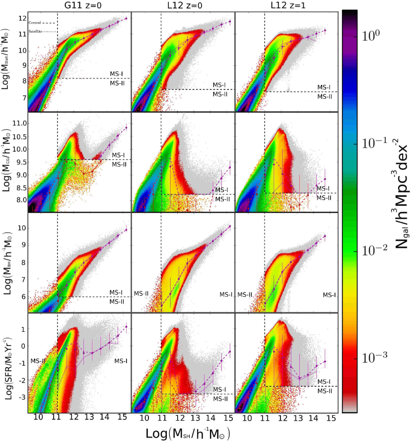
Figure 5: The predicted distributions of physical galaxy properties with subhalo mass (stellar mass, top row; cold gas mass, second row; black hole mass, third row; star formation rate, bottom row). The first column shows the G11 model at $z=0$. The second and third columns show the L12 model at $z=0$ and $z=1$ respectively. The colour shading shows the number density of galaxies as indicated by the key on the right. The black dashed lines show the transition from the MS-I to MS-II predictions and are in different places for the two models. The points with error bars show the median property values and the 20-80^th percentile range. The median property values are also shown for central (dashed lines) and satellites (dotted lines).

4 Results

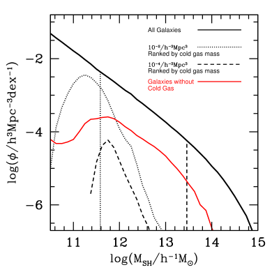
Figure 6: The subhalo mass function in the L12 model at $z=0$, constructed using all galaxies output by the model (solid black line in both panels). The vertical lines mark the masses above which the subhalos have abundances of $10^{-4}h^{3}{\rm Mpc}^{-3}$ (dashed line) and $10^{-2}h^{3}{\rm Mpc}^{-3}$ (dotted line). The other lines show the distribution of subhalo masses associated with the galaxies which pass a given selection criterion. In the top panel, the subhalo mass function is plotted for galaxies ranked in order of decreasing stellar mass, for an abundance of $10^{-4}h^{3}{\rm Mpc}^{-3}$ (dashed line) and $10^{-2}h^{3}{\rm Mpc}^{-3}$ (dotted line). In the bottom panel the same lines are used to show the subhalo mass function for the same galaxy number densities, but this time the galaxies have been ranked in terms of their cold gas mass. The solid red line shows the subhalo mass function for galaxies without any cold gas.

We now present the model predictions for how different galaxy properties depend on the mass of their host halo (§ 4.1), before looking more carefully into which halos contribute galaxies to different number density samples (§ 4.2). We then illustrate these dependencies further by attempt to reconstruct the SAM output by using the basic SHAM scheme (i.e. a subhalo abundance matching scheme without scatter) and a related approach (§4.3). Finally, in §4.4 we examine SHAM reconstruction at high redshift.

4.1 Subhalo mass - galaxy property distributions

We start by considering the predicted dependence of galaxy luminosity on host dark matter subhalo mass in the L12 model in Fig. 4. Galaxy luminosity in the optical was the original suggestion for a property that might display a monotonic dependence on halo mass (Vale & Ostriker 2004). The shading in Fig. 4 shows the abundance of galaxies as a function of their rest-frame $r$-band magnitude and host subhalo mass. As discussed in the previous section, we show predictions obtained from the MS-I and MS-II N-body runs, with the black dashed lines marking the transition from one set of results to the other, as labelled. The points and lines show the median $r$-band magnitude in bins of subhalo mass. The $r$-band magnitude shows a steep dependence on halo mass up to a mass of $\approx 10^{11.5}h^{-1}{\rm M_{\odot}}$. Beyond this mass the median $r$-band magnitude brightens less rapidly with increasing subhalo mass. This change in the slope of the median luminosity can be traced back to the onset of AGN heating of the hot gaseous halo, which stops gas cooling in halos more massive than $\approx 10^{11.5}h^{-1}{\rm M_{\odot}}$. Remarkably, there is essentially no difference in the median luminosity - halo mass relation when restricting attention to only central or satellite galaxies. The same trends are seen at $z=1$ and $z=4$.

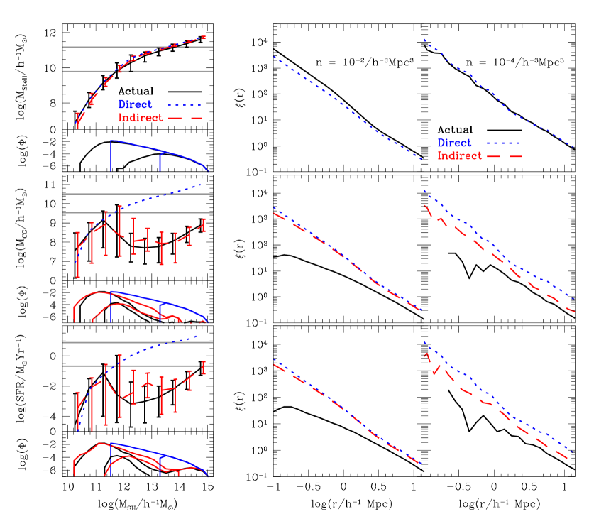
Figure 7: Tests of the accuracy of the reproduction of the actual galaxy sample predicted by the L12 model at $z=0$ using the direct and indirect SHAM reconstructions (see text). Each row shows the comparison for a different galaxy property (top - stellar mass; middle - cold gas mass; bottom - SFR). The main panels in the left column show the galaxy property - subhalo mass plane. The lines show the median galaxy property as a function of subhalo mass for the actual, direct and indirect samples as labelled. The lines showing the indirect samples have been shifted slightly for plotting clarity. The indirect curve is not shown in the top panel (stellar mass) since this is the same as the direct curve in this case. The 20-80^th percentile range is shown for the actual and indirect samples. The horizontal lines mark the property values in the actual sample which define the high (lower line) and low (upper line) density samples: it is the region of the plane above these lines which is of interest for these samples. The lower sub-panels show the distributions of subhalo masses in these cases. The second and third columns show the correlation functions measured for the samples as labelled for high and low densities, respectively.

The median galaxy luminosity - halo mass relation satisfies the central assumption behind SHAM, showing a monotonic dependence on host halo mass. However, Fig. 4 shows that there is considerable scatter when individual galaxies are considered. The 20-80^th percentile range covers almost two magnitudes at the subhalo mass where the relation changes slope. The full range of galaxy magnitudes predicted in the model is much wider, covering around $8$ magnitudes or a factor of 1500 in luminosity at the same mass. Similar results are found in other passbands. At longer wavelengths, galaxy luminosity is more closely related to stellar mass and the scatter in the luminosity - halo mass relation reduces slightly. At shorter wavelengths, the luminosity is driven more by the recent star formation history and also by the dust extinction, resulting in a more complicated dependence of luminosity on halo mass (see the discussion of SFR and luminosities at high-redshift in § 4.4).

Next we address the issue of the robustness of the SAM predictions by comparing the G11 and L12 models for different properties in Fig. 5. Here we focus on physical galaxy properties; stellar mass, cold gas mass, black hole mass and star formation rate. The left and middle columns compare the predictions of G11 and L12 respectively at $z=0$. If we first take the cases of stellar mass (top row) and black hole mass (third row down), the overall trends predicted by the two SAMs are similar, with more scatter predicted in the GALFORM case. GALFORM also predicts a higher scatter than L-GALAXIES when we consider galaxy luminosity. This is due to differences in the assumptions made to model galaxy formation physics, such as the choice of the time available for gas to cool from the hot halo. Observationally, the scatter in the halo mass - central galaxy luminosity relation has been studied using the dynamics of satellite galaxies (More et al. 2009, 2011). However, the question of whether or not the scatter predicted by either model is inconsistent with such observations remains open, as a careful comparison is required, repeating the analysis applied to the observations on a mock galaxy catalogue derived from the semi-analytical models, which is beyond the scope of the current paper. For both models, the stellar mass - halo mass relation changes slope at the halo mass at which AGN feedback starts to become important. Even though the models were calibrated to fit different datasets (primarily the stellar mass function in the case of G11 and the optical and near-infrared luminosity functions for L12), the change in slope occurs at approximately the same subhalo mass.

The predicted distributions for cold gas mass and star formation rate are closely related in G11, where all of the cold gas mass above some critical value is made available for star formation. In L12, only molecular hydrogen takes part in star formation, so there is no longer a direct link between the total cold gas mass and the star formation rate. Qualitatively, the cold gas - halo mass and SFR - halo mass distributions are similar for a given model. The distributions show the same features between models but are different in detail. At low halo masses, there is a reasonable correlation between cold gas and SFR and halo mass. This breaks down above the halo mass for which AGN feedback is important. The severity of the break is different in G11 and L12. This is because AGN feedback shuts down gas cooling completely in sufficiently massive halos in the L12 model, whereas the suppression of cooling is more gradual in G11. The relations between cold gas mass or SFR and subhalo mass are also different for central and satellite galaxies. Satellite galaxies are predicted to have lower median cold gas masses than centrals, with the difference being greater in L12 than in G11. This can be readily understood in terms of the differences in the treatment of cooling in satellites in the models. In L12, there is complete stripping of the hot halo when a galaxy becomes a satellite. In G11 the stripping of the hot gas is partial depending on the ram pressure experienced by the satellite as it orbits within the more massive halo.

Fig. 5 also shows the evolution of the galaxy property - halo mass distributions between $z=0$ and $z=1$ in the L12 model. There is little change in these distributions over this time interval. Although the abundance of massive dark matter halos changes appreciably between $z=4$ and $z=0$, the fraction of mass contained in halos with masses typical of those which host galaxies shows little change over this period (Mo & White 2002).

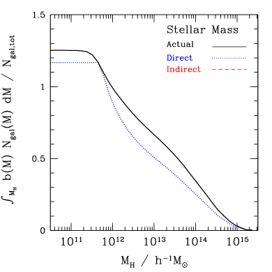
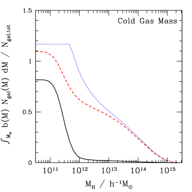
Figure 8: The contribution of different halos to the effective bias plotted as a function of halo mass, for galaxy samples with a number density of $10^{-2}h^{3}{\rm Mpc}^{-3}$ when ranked by their stellar mass (top panel) and by cold gas mass (botom panel) The black curve shows the bias in the actual sample. The asymptotic bias value at low halo masses gives the effective bias of the sample as $b_{\rm eff}=1.25$ for stellar mass and $b_{\rm eff}=0.82$ for the stellar mass sample. For the stellar mass case the SHAM reconstruction (blue curve) gives an effective bias of $b_{\rm eff}=1.18$ which is smaller than the actual bias. Note that there is no indirect curve in the top panel, since it has the same shape as the direct curve. The bottom panels shows that the effective bias for the reconstruction of the cold gas selected sample is higher than the actual effective bias, in agreement with the correlation function results shown in Fig. 7. The direct reconstruction effective bias curve flattens off at a halo mass of $4.5\times 10^{11}h^{-1}M_{\odot}$ since there no halos with masses below this in the direct sample.

4.2 Which subhalos contain galaxies?

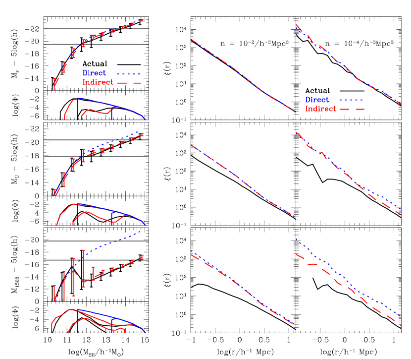
Figure 9: Same as Fig. 7, but this time the galaxy samples are defined by the magnitude in different bands: $r$-band (top), $U$-band (middle) and $1500$Å (bottom).

In the previous subsection we showed how galaxy properties are predicted to depend on subhalo mass. All of the properties considered display an appreciable scatter for a given halo mass. For some properties, such as cold gas mass and SFR, the dependence on subhalo mass is complex, which means that these galaxy properties are not good indicators of host halo mass. In this subsection we demonstrate the features of the model predictions by applying the basic SHAM hypothesis to reconstruct the SAM catalogues. We show the impact of this simple SHAM reconstruction by examining the range of halo masses populated with galaxies compared to that in the original catalogues, and the effect on the galaxy correlation function.

To gain some insight into the results presented later on in this section, we first examine which parts of the overall subhalo mass function are represented when different galaxy selections are made. Fig. 6 shows the subhalo mass function for subhalos associated with different galaxy samples for the L12 model at $z=0$. The solid black line shows the mass function when using the subhalos associated with all of the galaxies in the model output. This is our estimate of the “true” or complete subhalo mass function. We then build subsamples of galaxies by ranking them in terms of decreasing stellar mass (top panel) or cold gas mass (bottom panel) and plot the mass function of the associated subhalos. We do this for two galaxy number densities, $10^{-4}h^{3}{\rm Mpc}^{-3}$ (dashed lines) and $10^{-2}h^{3}{\rm Mpc}^{-3}$ (dotted lines). If a galaxy property satisfied the basic SHAM hypothesis exactly, then the mass function of the associated subhalos would include all of the available subhalos down to some mass, with a sharp transition to include zero subhalos of lower masses. This is indicated by for the two number densities by the vertical dashed and dotted lines in Fig. 6.

When galaxies are ranked in terms of their stellar mass, Fig. 6 shows that all of the subhalos above some mass are selected (e.g. a halo mass of $10^{12.6}h^{-1}{\rm M_{\odot}}$ for a galaxy abundance of $10^{-2}h^{3}{\rm Mpc}^{-3}$). However, due to the steepness of the halo mass function, the samples are dominated by somewhat lower halo masses, around $10^{11.4}h^{-1}{\rm M_{\odot}}$ in this case. At this mass, roughly half of the available subhalos are predicted to contain a galaxy which satisfies the cut in stellar mass which defines the sample. There is a tail of lower mass halos, extending roughly an order of magnitude in mass below the peak which also contribute. In these halos there is a declining chance (dropping to 1 in 10000 for the range of masses shown by the dotted line) that the halo contains a sufficiently massive galaxy.

The situation is more complex when galaxies are ranked by their cold gas mass. Fig. 6 shows that for both number density cuts, only a very small fraction of massive halos are represented. The peaks of the mass functions shown by the dotted and solid lines lie far below the overall subhalo mass function. This means that even for the most common subhalo mass present in the sample, only 1 in 3 halos (for the sample with space density $10^{-2}h^{3}{\rm Mpc}^{-3}$) or 1 in 100 halos (for the $10^{-4}h^{3}{\rm Mpc}^{-3}$ sample) make it into these catalogues. In the case of cold gas, it is much more likely that a massive subhalo (i.e. with mass $>10^{12}h^{-1}{\rm M_{\odot}}$) will contain galaxies with no cold gas (red line) than with enough cold gas to be selected. The presence of a sizable population of subhalos without cold gas is supported by a recent interpretation of the clustering strength of H I selected samples (Papastergis et al. 2013). Hence cold gas is not a suitable property to use in a direct basic SHAM analysis.

4.3 SHAM reconstruction of the SAM model predictions

We now apply the basic SHAM method (i.e. assuming no scatter in a galaxy property for a given subhalo mass) to reconstruct the L12 galaxy catalogue. We compare three types of galaxy catalogues as listed below:

• Actual: This is the catalogue predicted by the L12 SAM. Galaxies are ranked in terms of the galaxy property under consideration, in descending order of the property value. Two samples are used, corresponding to high ($10^{-2}h^{3}{\rm Mpc}^{-3}$) and low ($10^{-4}h^{3}{\rm Mpc}^{-3}$) space densities, corresponding to $1.25\times 10^{6}$ and $1.25\times 10^{4}$ galaxies respectively for the models run with MS-I.

• Direct: This is a reconstruction of the actual sample using the basic SHAM approach. The entire actual catalogue is effectively used to generate two ranked order lists: one ordered in terms of declining subhalo mass and the other in terms of the galaxy property under consideration. Galaxies are then assigned a subhalo mass determined by their position in the rank-ordered list i.e. the galaxy with the largest property value is assigned to the most massive subhalo and so-on down the list until the desired space density is attained.

• Indirect: This is a two step process in which SHAM is first applied to obtain the galaxy stellar mass. In the second step the target galaxy property is assigned by drawing from the distribution of the property as a function of stellar mass as predicted by the SAM (see Rodríguez-Puebla et al. 2011). In practice, when the galaxies are sorted in terms of their stellar mass, the associated values of the other galaxy properties predicted by the model are remembered. We then assign the value of a particular property that is associated with the galaxy, given its position in the list that is rank-ordered in terms of stellar mass. This approach can also be used to include scatter in the predicted galaxy property - subhalo mass distribution (though not in the case of the stellar mass, unless a different property is used in the first SHAM step to generate a rank-ordered list). By construction, for galaxies selected by stellar mass, the indirect and the direct samples will be identical.

  The main motivation for introducing the indirect approach is to improve the reproduction of the distribution of galaxies in the galaxy property - subhalo mass plane, particularly for galaxy properties which have a complex dependence on subhalo mass, such as the cold gas mass.

  The clustering signal in different samples is presented as an illustration of how the reconstruction method changes the relation between galaxies and their host dark matter halos (ie the main subhalo in the case of satellite galaxies). This is a challenging test of the reconstruction, as applying SHAM blurs any relation that is present in the semi-analytical model output between galaxy properties and local density, as a subhalo loses memory of whether it was originally a subhalo within a more massive halo or an isolated halo.

Here we have an advantage over studies which apply SHAM to reproduce galaxy clustering measured from observations in that we know the true or actual (using the terminology introduced above) subhalo mass attached to each galaxy, as predicted by the SAM. We judge how well the reproduction works by comparing the mass function of subhalos in the reconstructed sample to that in the actual sample and also by comparing the galaxy correlation function. If the reconstruction puts galaxies into the correct subhalos (i.e. those originally predicted by the SAM) then the galaxy correlation function will match that of the actual sample.

The tests of the quality of the reproduction of the L12 model are shown in Fig. 7 where each row shows the results for a different physical property (top row - stellar mass, second row - cold gas mass, third row - star formation rate). The main panels in the left-hand column show the galaxy property - halo mass distribution, as quantified through the median property values and the 20 - 80^th percentile distribution. The medians are shown for each catalogue: actual, direct and indirect. The horizontal lines in these panels show the minimum property values that define the two actual samples: the upper line is for the low space density sample and the lower line is for the high space density case. This shows which part of the galaxy property - subhalo mass plane contributes to these samples. The lower sub-panel in the left column of Fig. 7 shows the distribution of subhalo masses attached to the galaxies in each sample. Finally, the other columns show the comparison of the two-point galaxy correlation function for the high density (middle) and low density sample (right).

Starting with stellar mass (top panel), Fig. 7 shows that the direct SHAM approach gives a reasonable reproduction of the median stellar mass in the actual sample, returning median stellar masses that agree well with those in the actual sample for halo masses below $10^{12}h^{-1}{\rm M_{\odot}}$ and that are $\approx 0.2$ dex too high at higher subhalo masses. Note that for the stellar mass the indirect curve is not shown since it is identical to the direct curve; the median relation for the indirect method is plotted using bins that have been shifted slightly for clarity. The width of the distribution of stellar masses is smaller in the reconstructed samples than in the “actual” catalogue. The actual sample contains galaxies in lower mass subhalos than the simple SHAM reconstructions.

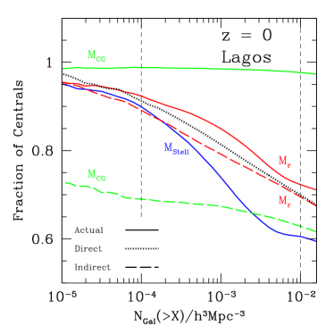
Figure 10: The fraction of central galaxies for different galaxy selections plotted as a function of the number density of galaxies in the sample, which corresponds to reducing the value of the property which is used to define the sample. The dotted black line shows the fraction of “central” subhalos in the direct sample. Different line colours and styles refer to different selections as indicated.

Out of all the properties we have studied, stellar mass is the only one for which the direct SHAM reconstruction leads to an underprediction of the correlation function (for the $10^{-2}h^{3}Mpc^{-3}$ density cut). In this case, the direct approach puts galaxies into lower mass subhalos than in the actual sample, as shown in the top panel of Fig. 8. This behaviour is critically dependent on the fraction of the subhalos of a given mass that are occupied, as shown in Fig. 6.

We now consider the impact of the reconstruction on the predicted clustering. The relevant part of the stellar mass - subhalo plane to focus on now is that above the horizontal lines in the top-left panel. In this case, all three catalogues show very similar distributions of subhalo masses (as shown by the lower left panel in this row). The clustering predictions are extremely close to one another for the low density sample. For the high density sample, the reconstructions predict a slightly lower clustering amplitude, with the discrepancy reaching $\approx 60\%$ on small scales.

The reconstructions work less well in the case of samples defined by their cold gas mass, as shown by the second row of Fig. 7. Applying the direct SHAM approach results in a monotonic relation between cold gas mass and subhalo mass. The predicted distribution in the actual sample is very different. There are three values of the subhalo mass compatible with a median cold gas mass of $\approx 10^{8}h^{-1}{\rm M_{\odot}}$ in the case of the actual sample. The direct approach puts galaxies into more massive subhalos than the model predicts. The indirect, two-step approach does a much better job of putting galaxies in subhalos of the correct mass and matching the width of the cold gas mass distribution. However, the clustering signal predicted by the reconstructions is much higher than the actual prediction, particularly for the high density sample. Remember, for the two samples under consideration we are only interested in the region of the cold gas - subhalo mass plane which lies above the horizontal lines. For the actual and indirect samples, the median cold gas mass is always below these lines, so we are focusing on the extremes of the distribution. Similar behaviour is found for the case of the SFR, as shown by the bottom row in Fig. 7.

Fig. 7 shows that the clustering in the reconstructions for samples defined by cold gas mass is higher than the prediction in the SAM. The contribution to the effective bias as function of halo mass is shown in the bottom panel of Fig. 8. The curve for the “actual” sample is always below those for the reconstructions, which means that the reconstructions preferentially populate higher mass subhalos with galaxies than is the case in the actual sample. The difference in the effective bias between the samples matches the difference seen in the two-halo term in the correlation function in Fig. 7.

Fig. 9 shows the results of the reconstruction of samples defined by galaxy luminosity in different bands. The top row shows the $r$-band (effective wavelength $\lambda_{\rm eff}=6166$ Å), the middle the $U$-band ($\lambda_{\rm eff}=3509$ Å) and the bottom row is for a rest frame wavelength of $1500$ Å. For the high density sample, the correlation function obtained from the reconstructions (direct and indirect) agrees well with that for the actual sample. For this density cut the $r$-band is the one the one that shows the best agreement with the direct reconstruction. For the low density sample, the clustering in the reconstructions is somewhat higher than in the actual sample, particularly on small scales. The $U$-band is more sensitive to the SFR and also to the dust extinction in the galaxy. The direct reconstruction does not work well in this case for subhalos more massive than $10^{11.8}h^{-1}{\rm M_{\odot}}$, predicting a median galaxy magnitude that is around one magnitude brighter than in the actual catalogue for massive halos. The indirect approach fares better. Nevertheless, both reconstructions overpredict the amplitude of the correlation function. Fig. 9 shows that the largest discrepancy between the reconstructions and the actual sample is found in the far-ultraviolet at $1500$ Å. The median magnitude has a nonmonotonic dependence on halo mass in the actual sample. This is reproduced reasonably well in the indirect reconstruction. However, by construction, this behaviour cannot be obtained from the direct approach. Neither of the reconstructions gives an accurate reproduction of the clustering in the actual sample. Although the indirect approach can reproduce the median magnitude - subhalo mass relation predicted in the actual sample, the number densities of galaxies under consideration means that it is the extreme of this distribution that is being probed in the clustering comparison. The reconstructions clearly do not reproduce the tails of the distributions.

Finally, we consider how the SHAM reconstruction affects the division between central and satellite galaxies. The number and spatial distribution of satellite galaxies in a halo shapes the form of the two-point correlation function on small scales and is referred to as the one-halo term. The largest differences seen in the correlation functions plotted in Fig. 7 and  9 occur on the scales sensitive to the one-halo term.

The SAM predicts which galaxies are centrals and which are satellites. In Fig. 10 we show the fraction of central galaxies predicted in the L12 model at $z=0$, as a function of the number density of the sample, when selecting using different galaxy properties. For the actual sample (solid line), the fraction of central galaxies shows similar behaviour when selecting on stellar mass or $r$-band magnitude. At low galaxy number densities, the samples are dominated by centrals, with the low-density sample containing around 90% centrals. The fraction of centrals drops with increasing galaxy number density, reaching 60% for stellar mass selection and 72% for $r$-band selection in the high density sample. However, when selecting on cold gas mass, the fraction of centrals is remarkably insensitive to the abundance of galaxies.

The designation in the SAM of a galaxy as a “central” or “satellite” can also be used to label the subhalo hosting the galaxy. In the direct SHAM reconstruction, we can track the fraction of the “central” subhalos after the halos are rank-ordered in mass. This is shown by the black dotted curve in Fig. 10. This curve has a similar shape to that predicted by the SAM for stellar mass and $r$-band selection. Hence we would expect the direct SHAM reconstruction of galaxy samples defined by these properties to produce similar numbers of central and satellite galaxies as predicted in the actual sample. This is not the case for cold gas selection, with the direct SHAM reconstruction predicting many more satellites than the model contains (comparing the black and green lines in Fig. 10).

The dashed line in Fig. 10 shows the fraction of centrals in the indirect SHAM reconstructions. The fraction of centrals in the $r$-band reconstruction is slightly lower than in the actual L12 predictions, but shows a similar trend with galaxy number density. The sample reconstructed using cold gas mass shows a much lower fraction of central galaxies, indicating that the indirect SHAM puts more galaxies into subhalos which were originally satellite subhalos, instead of putting them into central subhalos. This boosts the amplitude of the one-halo term in the correlation function. This is consistent with the results shown for the effective bias of these samples in Fig. 8.

4.4 Applying SHAM at high-redshift

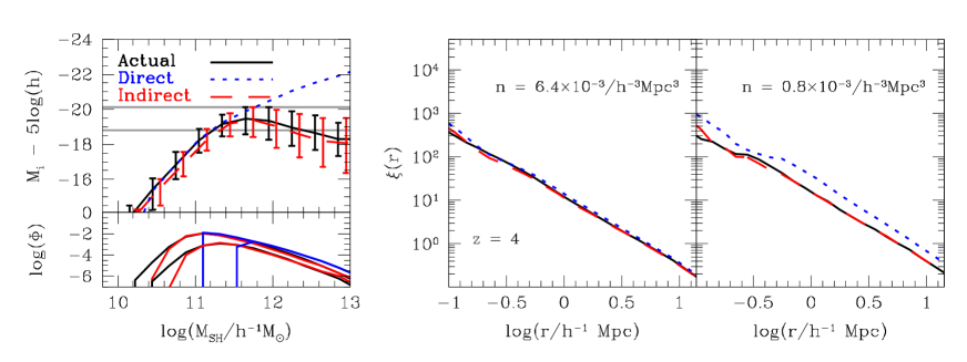
Figure 11: An application of SHAM at $z=4$, in a similar format to Figs. 7 and 9. Here galaxies are ranked by their observer-frame $i$-band magnitude. Density cuts of $0.8\times 10^{-3}h^{-3}{\rm Mpc}^{3}$ and $6.4\times 10^{-3}h^{-3}{\rm Mpc}^{3}$ are used to match the sample selection adopted by Conroy et al. (2006). The main panel in the left column shows the distribution in the $i-$band magnitude - subhalo mass plane, with the lower panel showing the abundance of haloes in each sample. The middle and right panels show the correlation function in the two galaxy samples, as labelled.

We now apply the basic SHAM scheme to reconstruct the L12 model predictions at $z=4$. The objective is to test the application of the basic SHAM technique to model the clustering of Lyman-break galaxies used by Conroy, Wechsler & Kravtsov (2006). The observational sample considered by Conroy et al. was selected in the observer-frame $i$ band, which, at this redshift probes an effective rest-frame wavelength of $\approx 1600$Å. The third row of Fig. 9 shows a similar test at $z=0$ and indicates that galaxy luminosity in the far ultra-violet is not a suitable property to use in a basic SHAM scheme, unless a fortuitous choice of galaxy number density is made. The comparison of the actual sample and the SHAM reconstructions is shown in Fig. 11, which is in the same format as Figs. 7 and 9. The left panel of Fig. 11 shows that the L12 model predicts a non-monotonic dependence of $i$-band magnitude on subhalo mass. The direct SHAM reconstruction overpredicts the brightness of galaxies hosted by massive halos. The upper of the two horizontal lines in Fig. 11 shows that this will be a problem for the low-density sample. The indirect approach reproduces the median $i$-band magnitude as a function of halo mass much better, albeit with a slightly larger scatter for massive subhalos. The lower panel shows that the direct SHAM puts galaxies into more massive subhalos than predicted by the actual sample. The right panel shows that this results in an overprediction of the clustering amplitude using the direct SHAM approach for the low density sample. The indirect approach, on the other hand, gives a good reproduction of the actual clustering. The SHAM reconstructions both reproduce the clustering in the actual catalogue for the higher number density sample. The left panel of Fig. 11 shows why this is the case. The lower of the two horizontal lines shows the $i$-band magnitude which is the selection limit for the high number density sample. This line intersects the actual, direct and indirect curves at the same place. Due to the steepness of the galaxy luminosity function and the subhalo mass function, it is this agreement which matters for the accuracy of the reproduction of the sample, as galaxies with luminosities close to this limit dominate. The disagreement between the actual and direct samples for higher subhalo masses does not matter in this case, as this only affects a small fraction of the overall sample.

In summary, the direct basic SHAM approach will not work for low density galaxy samples when the relation between galaxy property and subhalo mass is not monotonic. If a sufficiently high number density sample is considered, then SHAM will work provided that galaxies in low mass subhalos dominate the sample (by number). A similar conclusion regarding the inappropriateness of applying SHAM to ultra-violet selected samples was reached in a study of close pairs of galaxies by Berrier & Cooke (2012).

5 Summary and Conclusions

We have explored the connection between the mass of dark matter subhaloes and the properties of the galaxies they contain, using physically motivated models of galaxy formation. If a simple, deterministic relation holds, this motivates the development of empirical models of the galaxy population, such as subhalo abundance matching (SHAM).

The key assumption behind the original SHAM scheme (i.e. a scheme without scatter) is that there is a unique connection between a galaxy property and the mass of the galaxy’s host dark matter halo. We have explored this assumption studing the galaxy - dark matter halo connection in two independent, physically motivated models of galaxy formation. By using semi-analytical models implemented in the Millennium I and II N-body simulations (Guo et al. 2011; Lagos et al. 2012), we have been able to extend previous tests of SHAM well into the range of halo masses in which gas cooling is reduced by heating from active galactic nuclei (Simha et al. 2012). This is a critical point as many of the most significant discrepancies from the basic SHAM assumption are found in massive halos. Another advantage of our study is the use of galaxy merger histories to track the mass of halos at the point of infall into a more massive halo. In this way we are able to include subhalos which are no longer identifiable in a single output of an N-body simulation.

We have considered a range of intrinsic galaxy properties (stellar mass, cold gas mass, star formation rate, black hole mass) and direct observables (the luminosity in different bands, from the far ultra-violet to the optical). The model predictions show that none of these properties satisfy the basic SHAM assumption. Whilst some properties (stellar mass, black hole mass, $r$-band magnitude) display median values which vary monotonically with halo mass, a range of values is found for each halo mass. The models admittedly predict somewhat different ranges of property values, so the precise width of the distribution of values is a less robust model prediction. Some of this difference can be traced to choices made in the semi-analytical models (e.g. the definition of the time available for gas cooling). For other properties (cold gas mass, star formation rate, luminosity in the ultra-violet) the variation of the median with halo mass is complex. For some property values in these cases, galaxies could appear in very different mass halos.

The availability of the predictions of the galaxy formation models means that we can test how accurately SHAM can reconstruct the original catalogue. This exercise allows us to gain an impression of how the model predictions differ from the assumptions made in the simplest incarnations of SHAM. If the real Universe looks like the galaxy formation models, then this process will inform us about possible systematic errors when using simple SHAM schemes to model observed galaxy clustering. We judge the quality of the reproduction in terms of the median and percentile range of galaxy property in bins of subhalo mass and in terms of the two-point galaxy correlation function. The direct SHAM reconstructions tend to put galaxies with too high a value of the property under consideration into massive subhalos. This in turn results in the clustering being too high in low-density galaxy samples, compared with the prediction in the model. The direct reconstruction fares better at lower subhalo masses, which are not affected by AGN feedback. Hence for high number density galaxy samples, which are dominated by galaxies in lower mass subhalos, SHAM tends to give a better reproduction of the predicted clustering.

Extensions to the original SHAM proposal have been introduced to account for the scatter in the value of a galaxy property for a given subhalo mass and also to model properties which themselves are not thought to have a monotonic dependence on subhalo mass galaxy properties (Tasitsiomi et al. 2004; Behroozi, Conroy & Wechsler 2010; Moster et al. 2010; Rodríguez-Puebla et al. 2011; Hearin et al. 2013; Gerke et al. 2013; Masaki, Lin & Yoshida 2013; Hearin et al. 2014; Rodriguez-Puebla et al. 2014). Here we explore a simple variation on the basic SHAM scheme, which involves applying SHAM to one property and then assign galaxies a second property using a model which connects the two properties. The semi-analytical models predict the subhalo mass which hosts a galaxy, along with its intrinsic physical properties (e.g. stellar mass, cold gas mass, star formation rate). To build a sample for a property which does not have a simple dependence on host halo mass, we use a two-step approach. First, SHAM is applied to a galaxy property which does have a more straight forward relation to subhalo mass, as we found to be the case for stellar mass. Then to construct a sample which includes information about the desired galaxy property, for example the cold gas mass, we use the distribution of cold gas mass to stellar mass predicted by the semi-analytical model (see Appendix). We found this two step approach to be successful at reproducing the median and 20-80 percentile range of the target galaxy property as a function of subhalo mass. However, this approach does not always lead to the reproduction of the clustering signal in the model, particular for galaxy samples with a low number density. An extension to this approach could take into account the formation histories of the dark matter subhalos when assigning galaxy properties (Gao, Springel & White 2005; Wang, De Lucia & Weinmann 2013).

Appendix A Predictions for dependence of selected galaxy properties on stellar mass

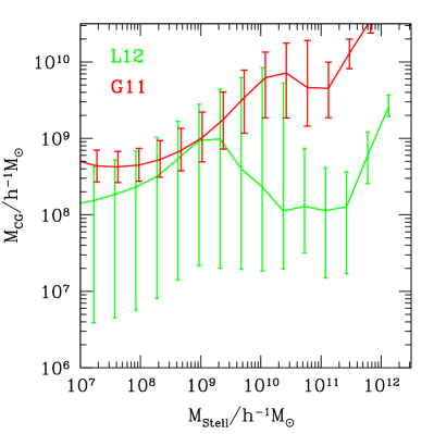
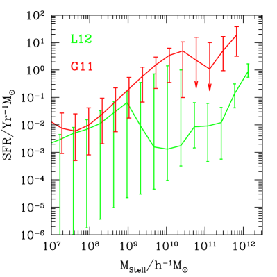
Figure 12: The predicted dependence of cold gas mass (top) and star formation rate (bottom) on stellar mass in the G11 (red) and L12 (green) models. The lines show the median value and the bars show the 20-80% percentile range. The downwards pointing arrow in the bottom plot means that the 20^thpercentile of the distribution has zero SFR.

Motivated by the predictions of the galaxy formation model, we consider an indirect, two-step SHAM approach in which galaxies are assigned a property based on their stellar mass. This requires knowledge of how the desired or target galaxy property depends on stellar mass. Fig. 12 shows the G11 and L12 model predictions for the dependence of cold gas mass (top) and star formation rate (bottom) on stellar mass. This information could be used in the indirect SHAM approach to build galaxy samples which cold gas information. Note that the models have not been calibrated to reproduce the same observations, hence the differences in these predictions. The L12 model predicts more scatter in cold gas mass and star formation rate for a given stellar mass than the G11 model.

References

- Baldry, Glazebrook & Driver (2008) Baldry I. K., Glazebrook K., Driver S. P., 2008, MNRAS, 388, 945
- Balogh et al. (2004) Balogh M. L., Baldry I. K., Nichol R., Miller C., Bower R., Glazebrook K., 2004, ApJL, 615, L101
- Baugh (2006) Baugh C. M., 2006, Reports on Progress in Physics, 69, 3101
- Baugh (2013) Baugh C. M., 2013, Pub. Aus. Astr. Soc., 30, 30
- Behroozi, Conroy & Wechsler (2010) Behroozi P. S., Conroy C., Wechsler R. H., 2010, ApJ, 717, 379
- Behroozi et al. (2014) Behroozi P. S., Wechsler R. H., Lu Y., Hahn O., Busha M. T., Klypin A., Primack J. R., 2014, ApJ, 787
- Benson (2010) Benson A. J., 2010, PhysRep, 495, 33
- Benson et al. (2003) Benson A. J., Bower R. G., Frenk C. S., Lacey C. G., Baugh C. M., Cole S., 2003, ApJ, 599, 38
- Benson et al. (2002) Benson A. J., Lacey C. G., Baugh C. M., Cole S., Frenk C. S., 2002, MNRAS, 333, 156
- Berrier & Cooke (2012) Berrier J. C., Cooke J., 2012, MNRAS, 426, 1647
- Bower et al. (2006) Bower R. G., Benson A. J., Malbon R., Helly J. C., Frenk C. S., Baugh C. M., Cole S., Lacey C. G., 2006, MNRAS, 370, 645
- Boylan-Kolchin et al. (2009) Boylan-Kolchin M., Springel V., White S. D. M., Jenkins A., Lemson G., 2009, MNRAS, 398, 1150
- Campbell et al. (2014) Campbell D. J. R. et al., 2014, ArXiv e-prints
- Cattaneo et al. (2006) Cattaneo A., Dekel A., Devriendt J., Guiderdoni B., Blaizot J., 2006, MNRAS, 370, 1651
- Cole et al. (2000) Cole S., Lacey C. G., Baugh C. M., Frenk C. S., 2000, MNRAS, 319, 168
- Conroy & Wechsler (2009) Conroy C., Wechsler R. H., 2009, ApJ, 696, 620
- Conroy, Wechsler & Kravtsov (2006) Conroy C., Wechsler R. H., Kravtsov A. V., 2006, ApJ, 647, 201
- Contreras et al. (2013) Contreras S., Baugh C. M., Norberg P., Padilla N., 2013, MNRAS, 432, 2717
- Crain et al. (2009) Crain R. A. et al., 2009, MNRAS, 399, 1773
- Croton et al. (2006) Croton D. J. et al., 2006, MNRAS, 365, 11
- Davis et al. (1985) Davis M., Efstathiou G., Frenk C. S., White S. D. M., 1985, ApJ, 292, 371
- De Lucia & Blaizot (2007) De Lucia G., Blaizot J., 2007, MNRAS, 375, 2
- De Lucia, Kauffmann & White (2004) De Lucia G., Kauffmann G., White S. D. M., 2004, MNRAS, 349, 1101
- Dutton et al. (2010) Dutton A. A., Conroy C., van den Bosch F. C., Prada F., More S., 2010, MNRAS, 407, 2
- Eke et al. (2005) Eke V. R., Baugh C. M., Cole S., Frenk C. S., King H. M., Peacock J. A., 2005, MNRAS, 362, 1233
- Faber & Jackson (1976) Faber S. M., Jackson R. E., 1976, ApJ, 204, 668
- Finkelstein et al. (2015) Finkelstein S. L. et al., 2015, ArXiv e-prints
- Font et al. (2008) Font A. S. et al., 2008, MNRAS, 289, 1619
- Gao, Springel & White (2005) Gao L., Springel V., White S. D. M., 2005, MNRAS, 363, L66
- Gerke et al. (2013) Gerke B. F., Wechsler R. H., Behroozi P. S., Cooper M. C., Yan R., Coil A. L., 2013, ApJS, 208, 1
- Ghigna et al. (1998) Ghigna S., Moore B., Governato F., Lake G., Quinn T., Stadel J., 1998, MNRAS, 300, 146
- Gonzalez-Perez et al. (2014) Gonzalez-Perez V., Lacey C. G., Baugh C. M., Lagos C. D. P., Helly J., Campbell D. J. R., Mitchell P. D., 2014, MNRAS, 439, 264
- Guo & White (2014) Guo Q., White S., 2014, MNRAS, 437, 3228
- Guo et al. (2011) Guo Q. et al., 2011, MNRAS, 413, 101
- Guo et al. (2010) Guo Q., White S., Li C., Boylan-Kolchin M., 2010, MNRAS, 404, 1111
- Hearin & Watson (2013) Hearin A. P., Watson D. F., 2013, MNRAS, 435, 1313
- Hearin et al. (2014) Hearin A. P., Watson D. F., Becker M. R., Reyes R., Berlind A. A., Zentner A. R., 2014, MNRAS, 444, 729
- Hearin et al. (2013) Hearin A. P., Zentner A. R., Berlind A. A., Newman J. A., 2013, MNRAS, 433, 659
- Jiang et al. (2014) Jiang L., Helly J. C., Cole S., Frenk C. S., 2014, MNRAS, 440, 2115
- Klypin et al. (2013) Klypin A., Prada F., Yepes G., Hess S., Gottlober S., 2013, ArXiv e-prints
- Kravtsov, Vikhlinin & Meshscheryakov (2014) Kravtsov A., Vikhlinin A., Meshscheryakov A., 2014, ArXiv e-prints
- Kravtsov, Gnedin & Klypin (2004) Kravtsov A. V., Gnedin O. Y., Klypin A. A., 2004, ApJ, 609, 482
- Lagos et al. (2011) Lagos C. D. P., Baugh C. M., Lacey C. G., Benson A. J., Kim H.-S., Power C., 2011, MNRAS, 418, 1649
- Lagos et al. (2012) Lagos C. d. P., Bayet E., Baugh C. M., Lacey C. G., Bell T. A., Fanidakis N., Geach J. E., 2012, MNRAS, 426, 2142
- Lagos, Cora & Padilla (2008) Lagos C. D. P., Cora S. A., Padilla N. D., 2008, MNRAS, 388, 587
- Masaki, Lin & Yoshida (2013) Masaki S., Lin Y.-T., Yoshida N., 2013, MNRAS, 436, 2286
- McCarthy et al. (2008) McCarthy I. G., Frenk C. S., Font A. S., Lacey C. G., Bower R. G., Mitchell N. L., Balogh M. L., Theuns T., 2008, MNRAS, 383, 593
- Merson et al. (2013) Merson A. I. et al., 2013, MNRAS, 429, 556
- Mo & White (2002) Mo H. J., White S. D. M., 2002, MNRAS, 336, 112
- Mocz et al. (2012) Mocz P., Green A., Malacari M., Glazebrook K., 2012, MNRAS, 425, 296
- More et al. (2009) More S., van den Bosch F. C., Cacciato M., Mo H. J., Yang X., Li R., 2009, MNRAS, 392, 801
- More et al. (2011) More S., van den Bosch F. C., Cacciato M., Skibba R., Mo H. J., Yang X., 2011, MNRAS, 410, 210
- Moster et al. (2010) Moster B. P., Somerville R. S., Maulbetsch C., van den Bosch F. C., Macciò A. V., Naab T., Oser L., 2010, ApJ, 710, 903
- Neistein et al. (2011) Neistein E., Li C., Khochfar S., Weinmann S. M., Shankar F., Boylan-Kolchin M., 2011, MNRAS, 416, 1486
- Nuza et al. (2013) Nuza S. E. et al., 2013, MNRAS, 432, 743
- Papastergis et al. (2013) Papastergis E., Giovanelli R., Haynes M. P., Rodríguez-Puebla A., Jones M. G., 2013, ApJ, 776, 43
- Peng et al. (2010) Peng Y.-j. et al., 2010, ApJ, 721, 193
- Reddick et al. (2013) Reddick R. M., Wechsler R. H., Tinker J. L., Behroozi P. S., 2013, ApJ, 771, 30
- Rodríguez-Puebla et al. (2011) Rodríguez-Puebla A., Avila-Reese V., Firmani C., Colín P., 2011, RMXAA, 47, 235
- Rodriguez-Puebla et al. (2014) Rodriguez-Puebla A., Avila-Reese V., Yang X., Foucaud S., Drory N., Jing Y. P., 2014, ArXiv e-prints
- Schaye et al. (2010) Schaye J. et al., 2010, MNRAS, 402, 1536
- Schaye & et al. (2014) Schaye J., et al., 2014, ArXiv e-prints
- Shankar et al. (2006) Shankar F., Lapi A., Salucci P., De Zotti G., Danese L., 2006, ApJ, 643, 14
- Simha & Cole (2013) Simha V., Cole S., 2013, MNRAS, 436, 1142
- Simha et al. (2012) Simha V., Weinberg D. H., Davé R., Fardal M., Katz N., Oppenheimer B. D., 2012, MNRAS, 423, 3458
- Simha et al. (2009) Simha V., Weinberg D. H., Davé R., Gnedin O. Y., Katz N., Kereš D., 2009, MNRAS, 399, 650
- Somerville (2002) Somerville R. S., 2002, ApJ, 572, L23
- Springel et al. (2005) Springel V. et al., 2005, Nature, 435, 629
- Springel et al. (2001) Springel V., White S. D. M., Tormen G., Kauffmann G., 2001, MNRAS, 328, 726
- Tasitsiomi et al. (2004) Tasitsiomi A., Kravtsov A. V., Wechsler R. H., Primack J. R., 2004, ApJ, 614, 533
- Trujillo-Gomez et al. (2011a) Trujillo-Gomez S., Klypin A., Primack J., Romanowsky A. J., 2011a, ApJ, 742, 16
- Trujillo-Gomez et al. (2011b) Trujillo-Gomez S., Klypin A., Primack J., Romanowsky A. J., 2011b, ApJ, 742, 16, 24 pp
- Tully & Fisher (1977) Tully R. B., Fisher J. R., 1977, A&A, 54, 661
- Tully et al. (1998) Tully R. B., Pierce M. J., Huang J.-S., Saunders W., Verheijen M. A. W., Witchalls P. L., 1998, AJ, 115, 2264
- Vale & Ostriker (2004) Vale A., Ostriker J. P., 2004, MNRAS, 353, 189
- Vale & Ostriker (2006) Vale A., Ostriker J. P., 2006, MNRAS, 371, 1173
- Verheijen (1997) Verheijen M. A. W., 1997, PhD thesis, Univ. Groningen, The Netherlands
- Vogelsberger et al. (2014) Vogelsberger M. et al., 2014, Nature, 509, 177
- Wake et al. (2011) Wake D. A. et al., 2011, ApJ, 728, 46
- Wang, De Lucia & Weinmann (2013) Wang L., De Lucia G., Weinmann S. M., 2013, MNRAS, 431, 600
- White & Rees (1978) White S. D. M., Rees M. J., 1978, MNRAS, 183, 341
- Yamamoto, Masaki & Hikage (2015) Yamamoto M., Masaki S., Hikage C., 2015, ArXiv e-prints