Iteratively reweighted adaptive lasso
for conditional heteroscedastic time series
with applications to AR-ARCH type processes

Abstract

Shrinkage algorithms are of great importance in almost every area of statistics due to the increasing impact of big data. Especially time series analysis benefits from efficient and rapid estimation techniques such as the lasso. However, currently lasso type estimators for autoregressive time series models still focus on models with homoscedastic residuals. Therefore, an iteratively reweighted adaptive lasso algorithm for the estimation of time series models under conditional heteroscedasticity is presented in a high-dimensional setting. The asymptotic behaviour of the resulting estimator is analysed. It is found that the proposed estimation procedure performs substantially better than its homoscedastic counterpart. A special case of the algorithm is suitable to compute the estimated multivariate AR-ARCH type models efficiently. Extensions to the model like periodic AR-ARCH, threshold AR-ARCH or ARMA-GARCH are discussed. Finally, different simulation results and applications to electricity market data and returns of metal prices are shown.

1 Introduction

High-dimensional shrinkage and parameter selection techniques are of increasing importance in statistics in the past years. In recent years, high-dimensional shrinkage and parameter selection techniques have been of increasing importance. In many statistical areas, lasso (least absolute shrinkage and selection operator) estimation methods, as introduced by Tibshirani, (1996), are very popular. In time series analysis the influence of lasso type estimators is growing, especially as the asymptotic properties of stationary time series are usually very similar for stationary time series to the standard regression case, see e.g. Wang et al., 2007b , Nardi and Rinaldo, (2011) and Yoon et al., (2013). Hence, given the lasso’s shrinkage properties, it is attractive for subset selection in autoregressive models. In big data settings, it provides an efficient estimation technique, see Hsu et al., (2008), Ren and Zhang, (2010), and Ren et al., (2013) for more details.

Unfortunately, almost the entire literature about $\ell_{1}$-penalised least square estimation, like the lasso, deals with homoscedastic models. The case of heteroscedasticity and conditional heteroscedasticity is rarely has rarely been covered so far. Recently, Medeiros and Mendes, (2012) showed that the adaptive lasso estimator is consistent and asymptotically normal under very weak assumptions. They proved that the consistency and the asymptotic normality hold if the residuals are described by a weak white noise process. This includes the case of conditional heteroscedastic ARCH and GARCH-type residuals. Nevertheless, their classical lasso approach does not make use of the structure of the conditional heteroscedasticity within the residuals. Without going into detail, it is clear that the estimators might be improved if the structure of the conditional heteroscedasticity in the data is used. Furthermore, Yoon et al., (2013) analysed the lasso estimator in an autoregressive regression model. Additionally, they formulated the lasso problem in a time series setting with ARCH errors. However, they did not provide a solution to the estimation problem and left this for future research.

Recently, Wagener and Dette, (2012) and Wagener and Dette, (2013) analysed the properties of weighted lasso-type estimators in a classical heteroscedastic regression setting. They showed that their estimators are consistent and asymptotically normal. In addition, their estimators perform significantly better than their homoscedastic counterpart. Their results, conditioned on the covariates, can be used to construct a reweighted estimator that also works in time series settings.

We derive an iteratively reweighted adaptive lasso algorithm that addresses the above mentioned problems. It enables the estimation of high-dimensional sparse time series models under conditional heteroscedasticity. We assume a regression structure which is satisfied by the majority of the important time series processes and which admits fast estimation methods. The computational complexity of the algorithm is essentially the same as the coordinate descent algorithm of Friedman et al., (2007). This very fast estimation method for convex penalised models, such as the given $\ell_{1}$ situation, can be applied to the iteratively reweighted adaptive lasso algorithm.

The algorithm is based on the results of Wagener and Dette, (2013), as their results can be generalised to models with conditional heteroscedasticity. The sign consistency and asymptotic normality for the proposed estimator is adduced. Furthermore, a general high-dimensional setting, where in which the underlying process might have an infinite amount of parameters, is considered. Note that all the time series results hold in a classical regression setting as well.

However, we restrict ourself to $\ell_{1}$-penalised regressions as they are popular in time series settings (see e.g. Wang et al., 2007b , Nardi and Rinaldo, (2011) and Yoon et al., (2013)). In general, other $\ell_{q}$-penalty could also be considered, e.g. the $\ell_{2}$ penalty. The $\ell_{2}$ penalty, which gives the ridge regression, is suitable for shrinkage as well, but does not allow for sparsity. However in $\ell_{q}$-penalised regression, the case $q=1$ is the greatest case of practical intereststill allowing for sparsity. This sparsity property can be used in applications to select the required tuning parameter based on information criteria that are popular in time series analysis.

The general problem ist stated in section 2. In section 3, we motivate and provide the estimation algorithm. Subsequently, the asymptotics are discussed in in section 4.In Section 5, an application to multivariate AR-ARCH type processes is considered. This includes several extensions such as periodic AR-ARCH, AR-ARCH with structural breaks, threshold AR-ARCH and ARMA-GARCH models. The section 6 shows simulation which underline the results given above. It provides evidence that incorporating the heteroscedasticity in a high-dimensional setting is more important than in low dimensional problems. Finally, we consider the proposed algorithm as a model for the electricity market and metal prices returns data. A two-dimensional AR-ARCH type model is used in both applications to the hourly data, in the first one to electricity price and load data and in the second one to gold and silver price returns.

2 The considered time series model

The considered model is basically similar to the one used by Yoon et al., (2013) or Medeiros and Mendes, (2012). Let $(Y_{t})_{t\in{\mathbb{Z}}}$ be the considered causal univariate time series. We assume that it follows the linear equation

$$Y_{t}=\boldsymbol{X}_{\infty,t}\boldsymbol{\beta}^{0}_{\infty}+{\varepsilon}_{t},$$ (1)

where $\boldsymbol{X}_{\infty,t}=(X_{1,t},X_{2,t},\ldots)$ is a possibly infinite vector of covariates of weakly stationary processes $(X_{i,t})_{t\in{\mathbb{Z}}}$, $({\varepsilon}_{t})_{t\in{\mathbb{Z}}}$ is an error process, and the parameter vector is $\boldsymbol{\beta}^{0}_{\infty}=(\beta^{0}_{1},\beta^{0}_{2},\ldots)^{\prime}$ with $\sum_{i=1}^{\infty}|\beta^{0}_{i}|<\infty$. The covariates can also contain lagged versions of $Y_{t}$, which allows flexible modelling of autoregressive processes.

A simple example of a process that helps for understanding this paper is an invertable seasonal MA(1) process. In particular, the AR($\infty$) representation of a seasonal MA(1) with seasonality $2$ is useful. It is given by $Y_{t}={\varepsilon}_{t}-\theta{\varepsilon}_{t-2}=\theta Y_{t-2}+\theta^{2}Y_{t-4}+\theta^{3}Y_{t-6}+\ldots+{\varepsilon}_{t}$, choosing $\boldsymbol{X}_{\infty,t}=(Y_{t-1},Y_{t-2},\ldots)$ with $\boldsymbol{\beta}_{\infty}^{0}=(0,\theta,0,\theta^{2},0,\theta^{3},0,\ldots)^{\prime}$. The error process $({\varepsilon}_{t})_{t\in{\mathbb{Z}}}$ is assumed to follow a zero mean process with $\epsilon_{t}$ being uncorrelated to the covariates $\boldsymbol{X}_{\infty,t}$. Hence we require ${\mathbb{E}}({\varepsilon}_{t})=0$ and $\operatorname{{\mathbb{C}}ov}({\varepsilon}_{t},X_{i,t})=0$ for all $i\in{\mathbb{N}}$. Moreover, we assume that ${\varepsilon}_{t}$ is a weak white noise process, such that

$${\varepsilon}_{t}=\sigma_{t}Z_{t}\text{ where }\sigma_{t}=g(\boldsymbol{\alpha}^{0}_{\infty};\boldsymbol{L}_{\infty,t})\text{ and }(Z_{t})_{t\in{\mathbb{Z}}}\text{ is i.i.d. with }{\mathbb{E}}(Z_{t})=0\text{ and }\operatorname{{\mathbb{V}}ar}(Z_{t})=1.$$ (2)

Here, $g$ is a positive function, $\boldsymbol{L}_{\infty,t}=(L_{1,t},L_{2,t},\ldots)$ is a possibly infinite vector of covariates of weakly stationary processes $(L_{i,t})_{t\in{\mathbb{Z}}}$, and $\boldsymbol{\alpha}^{0}_{\infty}=(\alpha^{0}_{1},\alpha^{0}_{2},\ldots)^{\prime}$ is a parameter vector. Similarly to the covariates $\boldsymbol{X}_{\infty,t}$ in (1), $\boldsymbol{L}_{\infty,t}$ can also include lags of $\sigma_{t}$ or ${\varepsilon}_{t}$. This allows for a huge class of popular conditional variance models, like ARCH or GARCH type models. Choosing

$$g(\boldsymbol{\alpha}^{0}_{\infty};\boldsymbol{L}_{\infty,t})=g((\alpha_{0},\alpha_{1},\ldots);({\varepsilon}_{t-1},\sigma_{t-1},0,\ldots))=\sqrt{\alpha_{0}+\alpha_{1}{\varepsilon}_{t-1}^{2}+\alpha_{2}\sigma_{t-1}^{2}}$$

leads to the very popular GARCH(1,1) process. Note that the introduced setting is more general than the conditional heteroscedastic problem stated by Yoon et al., (2013), who mentioned only ARCH errors.

For the following we assume that the time points $1$ to $n$ are observable for $Y_{t}$. Thus, we denote by

$$\boldsymbol{Y}_{n}=\left(\begin{array}[]{c}Y_{1}\\ \vdots\\ Y_{n}\end{array}\right),\boldsymbol{X}_{n}=\left(\begin{array}[]{ccc}X_{1,1}&\cdots&X_{1,p_{n}}\\ \vdots&\ddots&\vdots\\ X_{n,1}&\cdots&X_{n,p_{n}}\end{array}\right),\boldsymbol{\beta}_{n}=\left(\begin{array}[]{c}\beta_{1}\\ \vdots\\ \beta_{p_{n}}\end{array}\right)\text{, and }\boldsymbol{\varepsilon}_{n}=\boldsymbol{Y}_{n}-\boldsymbol{X}_{n}\boldsymbol{\beta}_{n}$$

the response vector $\boldsymbol{Y}_{n}$, the $n\times p_{n}$ matrix of the covariates $\boldsymbol{X}_{n}$, the parameter vector $\boldsymbol{\beta}_{n}$ and the corresponding errors $\boldsymbol{\varepsilon}_{n}$. Furthermore let $X_{1},\ldots,X_{n}$ be the rows of $\boldsymbol{X}_{n}$.

Since we deal with a high-dimensional setting we are interested in situations where the number of possible parameters $p_{n}$ increases with sample size $n$. Therefore, denote $\boldsymbol{\beta}^{0}_{n}=(\beta_{1}^{0},\ldots,\beta_{p_{n}}^{0})^{\prime}$ the restriction of $\boldsymbol{\beta}_{\infty}^{0}$ to its first $p_{n}$ coordinates. Due to $\sum_{i=1}^{\infty}|\beta^{0}_{i}|<\infty$ it follows for $\boldsymbol{\varepsilon}^{0}_{n}=({\varepsilon}_{n,1}^{0},\ldots,{\varepsilon}^{0}_{n,n})^{\prime}=\boldsymbol{Y}_{n}-\boldsymbol{X}_{n}\boldsymbol{\beta}^{0}_{n}$ that there is a positive decreasing sequence $(\zeta_{n})_{n}$ with $\zeta_{n}\to 0$ such that $\lim_{n\to\infty}P(\max_{1\leq t\leq n}|{\varepsilon}_{n,t}^{0}-{\varepsilon}_{t}|<\zeta_{n})\to 1$ holds. Thus, for a sufficiently large $n$ we can approximate $Y_{t}$ by $\boldsymbol{X}_{n,t}\boldsymbol{\beta}_{n}^{0}$ arbitrarily well.

However, under the assumption of sparsity, meaning that only some of the regressors attribute significantly to the model, we can conclude that only $q_{n}$ of the $p_{n}$ parameters are non-zero. Hence, there are $p_{n}-q_{n}$ parameters that are exactly zero. Without loss of generality we assume that $\boldsymbol{X}_{n}$ and $\boldsymbol{\beta}^{0}_{n}$ are arranged so that the first $q_{n}$ components of $\boldsymbol{\beta}^{0}_{n}$ are non-zero, whereas the following are zero. Obviously we have $\boldsymbol{\beta}^{0}_{n}=(\beta^{0}_{1},\ldots,\beta^{0}_{q_{n}},0,\ldots,0)^{\prime}=(\boldsymbol{\beta}^{0}_{n}(1)^{\prime},\boldsymbol{0}^{\prime})^{\prime}$. This arrangement of the non-zero components is only used to simplify the notation, it is especially not required by the estimation procedure. Additionally we introduce the naive partitioning of $\boldsymbol{X}_{n}$ and $\boldsymbol{\beta}_{n}$, in such a manner that $\boldsymbol{\beta}_{n}=(\boldsymbol{\beta}_{n}(1)^{\prime},\boldsymbol{\beta}_{n}(2)^{\prime})^{\prime}$, $\boldsymbol{X}_{n}=(\boldsymbol{X}_{n}(1),\boldsymbol{X}_{n}(2))$ and $\boldsymbol{X}_{n,t}=(\boldsymbol{X}_{n,t}(1)^{\prime},\boldsymbol{X}_{n,t}(2)^{\prime})^{\prime}$ holds.

Subsequently, we focus on the estimation of $\boldsymbol{\beta}_{n}^{0}$, for which we will utilize a lasso-based approach for $\boldsymbol{\beta}_{n}$. Henceforth, we achieve never a direct estimate for $\boldsymbol{\beta}^{0}_{\infty}$, but we can approximate it by $(\boldsymbol{\beta}_{n}^{\prime},\boldsymbol{0}^{\prime})^{\prime}$.

3 Estimation algorithm

The proposed algorithm is based on the classical iteratively reweighted least squares procedure. An example for an application of it to time series analysis can be found e.g. in Mak et al., (1997). However, similar approaches are not popular in time series modelling, as there are usually better alternatives if the number of parameters is small. In that case, we can simply perform an estimation of the joint likelihood function of (1), see e.g. Bardet et al., (2009). But when facing a high-dimensional problem, it is almost impossible to maximise the non-linear loss function with many parameters. In contrast, our algorithm can be based on the coordinate descent lasso estimation technique as suggested by Friedman et al., (2007) which provides a feasible and fast estimation technique. Other techniques, like the LARS algorithm introduced by Efron et al., (2004) which provides the full lasso solution path, can be used as well.

For motivating the proposed algorithm, we divide equation (1) by its volatility, resp. conditional standard deviation $\sigma_{t}$. Thus, we obtain

$$\widetilde{Y}_{t}=\widetilde{\boldsymbol{X}}_{\infty,t}\boldsymbol{\beta}_{\infty}+Z_{t},$$ (3)

where $\widetilde{Y}_{t}=\frac{1}{\sigma_{t}}{Y}_{t}$ and $\widetilde{\boldsymbol{X}}_{\infty,t}=\frac{1}{\sigma_{t}}{\boldsymbol{X}}_{\infty,t}$. Here, the noise $Z_{t}$ is homoscedastic with variance $1$. Hence, if the volatility $\sigma_{t}$ of the process $Y_{t}$ is known, we can simply apply common lasso time series techniques under homoscedasticity. Unfortunately, this is never the case in practice. The basic idea is now to replace $\sigma_{t}$ by a suitable estimator $\widehat{\sigma}_{t}$, which allows us to perform a lasso estimate on a homoscedastic time series as in equation (3).

For estimating ARMA-GARCH processes, practitioners sometimes use a multi-step estimator. This estimation technique involves computing ARMA parameters in a homoscedastic setting first and then use the resulting estimated residuals are used to estimate the GARCH part in a second step, see e.g. Mak et al., (1997) or Ling, (2007). We will apply a similar step-wise estimation technique here.

In general, we have no a priori information about $\sigma_{t}$, hence we should assume homoscedasticity in a first estimation step. We start with the estimation of the regression parameters $\boldsymbol{\beta}_{n}^{0}$, resp. $\boldsymbol{\beta}^{0}_{\infty}$, and obtain the residuals $\widehat{{\varepsilon}}_{n,1},\ldots,\widehat{{\varepsilon}}_{n,n}$. We use the residuals to estimate the conditional variance parameters $\boldsymbol{\alpha}^{0}_{\infty}$ and thus $(\sigma_{1},\ldots,\sigma_{n})$ by $(\widehat{\sigma}_{n,1},\ldots,\widehat{\sigma}_{n,n})$ afterwards. Afterwards, we reweight model (1) by $\widehat{\sigma}_{t}^{-1}$ to get a homoscedastic model version which we utilise in order to reestimate $\boldsymbol{\beta}_{n}^{0}$ again. We can use this new estimate of $\boldsymbol{\beta}^{0}_{n}$ to repeat this procedure. Thus, we will end up in an iterative algorithm that hopefully converges in some sense to $\boldsymbol{\beta}_{n}^{0}$, resp. $\boldsymbol{\beta}^{0}_{\infty}$, with increasing sample size $n$.

We use an adaptive weighted lasso estimator to estimate $\boldsymbol{\beta}^{0}_{n}$ within each iteration step. It is given by

$$\boldsymbol{\beta}_{n,\text{lasso}}(\lambda_{n},\boldsymbol{v}_{n},\boldsymbol{w}_{n})=\operatorname*{arg\,min}_{\boldsymbol{\beta}}\sum_{t=1}^{n}w_{n,t}^{2}\bigg{(}Y_{t}-\sum_{i=1}^{p_{n}}X_{t,i}\beta_{i}\bigg{)}^{2}+\lambda_{n}\sum_{j=1}^{p_{n}}v_{n,j}|\beta_{j}|$$

or in vector notation

$$\boldsymbol{\beta}_{n,\text{lasso}}(\lambda_{n},\boldsymbol{v}_{n},\boldsymbol{w}_{n})=\operatorname*{arg\,min}_{\boldsymbol{\beta}}(\boldsymbol{Y}_{n}-\boldsymbol{X}_{n}\boldsymbol{\beta})^{\prime}\boldsymbol{W}_{n}^{2}(\boldsymbol{Y}_{n}-\boldsymbol{X}_{n}\boldsymbol{\beta})+\lambda_{n}\boldsymbol{v}_{n}^{\prime}|\boldsymbol{\beta}|,$$

where $\boldsymbol{W}_{n}=\operatorname{diag}(\boldsymbol{w}_{n})$, $\boldsymbol{w}_{n}=(w_{n,1},\ldots,w_{n,n})$ are the heteroscedasticity weights, $\boldsymbol{v}_{n}=(v_{n,1},\ldots,v_{n,p_{n}})$ are the penalty weights and $\lambda_{n}$ is a penalty tuning parameter. As described above, in the iteratively reweighted adaptive lasso algorithm we have the special choice $\boldsymbol{w}_{n}=(w_{n,1},\ldots,w_{n,n})=(\widehat{\sigma}_{n,1}^{-1},\ldots,\widehat{\sigma}_{n,n}^{-1})$ for the heteroscedasticity weights within each iteration step. We require $\boldsymbol{w}_{n}=\boldsymbol{1}$ for the homoscedatic initial step.

Like Zou, (2006) we consider, for the tuning parameter $\boldsymbol{v}_{n}$, the choice $\boldsymbol{v}_{n}={\boldsymbol{\beta}}_{n,\text{init}}^{-\tau}$ for some $\tau\geq 0$ and some initial parameter estimate $\boldsymbol{\beta}_{n,\text{init}}$. With $\tau=0$ we obtain $\boldsymbol{v}_{n}=\boldsymbol{1}$ which is the usual lasso estimator. Obviously, there is no initial estimator required in this case. However, we consider the case of $\tau=0$ and the adaptive lasso approach for our practical application, as they resulted in different perfomances.

The selection of the tuning parameters $\lambda_{n}$ and $\tau$ such as the choice of the initial estimate ${\boldsymbol{\beta}}_{n,\text{init}}$ is crucial for the application and might demand some computational cost. We discuss this issue in more detail at the end of the next section.

Subsequently, we denote $\widehat{\boldsymbol{\alpha}}_{n}=\widehat{\boldsymbol{\alpha}}_{n}(\boldsymbol{\beta}_{n};\boldsymbol{X}_{n},\boldsymbol{Y}_{n})$ as a known plug-in estimator for $\boldsymbol{\alpha}_{n}^{0}$, which is the projection of $\boldsymbol{\alpha}_{\infty}^{0}$ to its first $l_{n}$ coordinates. We denote $g_{n}$ as restriction of $g$ that corresponds to $\boldsymbol{\alpha}_{n}^{0}$. Thus, $g_{n}$ is defined such that $\boldsymbol{\alpha}_{\infty}^{0}$ is restricted to $\boldsymbol{\alpha}_{n}^{0}$ and $\boldsymbol{L}^{0}_{n}$ is a restriction of $\boldsymbol{L}_{\infty}=(\boldsymbol{L}_{\infty,t})_{t\in{\mathbb{Z}}}$ to its first $m_{n}(l_{n})$ coordinates. Similarly, let $\widehat{\boldsymbol{L}}_{n}=\widehat{\boldsymbol{L}}_{n}(\boldsymbol{\beta}_{n};\boldsymbol{X}_{n},\boldsymbol{Y}_{n})$ be an estimator for $(\boldsymbol{L}^{0}_{n,1},\ldots,\boldsymbol{L}^{0}_{n,n})^{\prime}$.

For example, if ${\varepsilon}_{t}$ follows a GARCH(1,1) process we receive $\sigma_{t}=g_{n}(\boldsymbol{\alpha}_{n}^{0},\boldsymbol{L}_{n,t}^{0})$ for all $n\in{\mathbb{N}}$, where $\boldsymbol{\alpha}_{n}^{0}=(\alpha_{0},\alpha_{1},\alpha_{2})$ with $l_{n}=3$ and $\boldsymbol{L}_{n,t}^{0}=({\varepsilon}_{t-1},\sigma_{t-1})$ with $m_{n}(l_{n})=2$ for all $n\in{\mathbb{N}}$. This is similarly feasible for every variance model with a finite amount of parameters. However, if $\sigma_{t}$ follows an infinite parameterised process, e.g. through an ARCH($\infty$) process, $l_{n}$ and $m_{n}(l_{n})$ should tend to infinity as $n\to\infty$.

The estimation scheme of the described iteratively reweighted adaptive lasso algorithm is given by:

1. initialise $\lambda_{n}\geq 0$, $\boldsymbol{v}_{n}(\tau)=(v_{n,1}(\tau),\ldots,v_{n,p_{n}}(\tau))=\boldsymbol{\beta}_{n,\text{init}}^{-\tau}$ with $\tau\geq 0$ and $\boldsymbol{w}_{n}^{[0]}=\boldsymbol{1}$, $k=1$ 2. estimate by weighted lasso: $\boldsymbol{\beta}_{n}^{[k]}=\boldsymbol{\beta}_{n}^{[k]}(\boldsymbol{w}_{n}^{[k-1]})=\boldsymbol{\beta}_{n,\text{lasso}}(\lambda_{n},\boldsymbol{v}_{n}(\tau),\boldsymbol{w}_{n}^{[k-1]})$ 3. estimate the conditional variance model: $\boldsymbol{\alpha}_{n}^{[k]}=\widehat{\boldsymbol{\alpha}}_{n}(\boldsymbol{\beta}_{n}^{[k]};\boldsymbol{X}_{n},\boldsymbol{Y}_{n})$ and $\boldsymbol{L}_{n}^{[k]}=\widehat{\boldsymbol{L}}_{n}(\boldsymbol{\beta}_{n}^{[k]};\boldsymbol{X}_{n},\boldsymbol{Y}_{n})$ 4. compute new weights $\boldsymbol{w}^{[k]}_{n}=(\boldsymbol{w}_{n,1}^{[k]},\ldots,\boldsymbol{w}_{n,n}^{[k]})$ with $\boldsymbol{w}_{n,t}^{[k]}=g_{n}(\boldsymbol{\alpha}_{n}^{[k]},\boldsymbol{L}_{n,t}^{[k]})^{-1}$ 5. if the stopping criterion is not met, $k=k+1$ and back to 2. otherwise, return estimate $\boldsymbol{\beta}_{n}^{[k]}$ and volatilities $\widehat{\boldsymbol{\sigma}}_{n,t}^{[k]}=g_{n}(\boldsymbol{\alpha}_{n}^{[k]},\boldsymbol{L}^{[k]}_{n,t})$

We can summarise that we have to specify the tuning parameter $\lambda_{n}$, the initial estimator $\boldsymbol{\beta}_{n,\text{init}}$ with an inital value of $\tau$, and the initial heteroscedasticity weights $\boldsymbol{w}_{n}$. To reduce the computation time it can be convenient in practice to choose $\tau=0$ (lasso) or $\tau=1$ (almost non-negative garotte).

The stopping criterion in step 5 has to be chosen as well, such that the algorithm eventually stops. A plausible stopping criterion should measure the convergence of $\boldsymbol{w}_{n}^{[k]}$, resp. $\boldsymbol{\sigma}_{n}^{[k]}$. We suggest to stop the algorithm if $\|\boldsymbol{\sigma}_{n}^{[k]}-\boldsymbol{\sigma}_{n}^{[k-1]}\|<\epsilon$ for a selected vector norm $\|\cdot\|$ and some small $\epsilon>0$. Nevertheless, in our simulation study, we realised that the difference in the later steps are marginal, so that stopping at $k=2$ or $k=3$ seems to be reasonable for practice. This will be underlined by the asymptotics of the algorithm as analysed below; it can be shown that, under certain conditions, $k=2$ is sufficient to get an optimal estimator if $n$ is large.

4 Asymptotics of the algorithm

For the general convergence analysis it is clear that the asymptotic of the estimator $\boldsymbol{\beta}_{n}^{[k]}$ will strongly depend on the (cond.) heteroscedasticity models (2) (esp. the formula for $g$) such as on the linked estimators $\widehat{\boldsymbol{\alpha}}_{n}$ and $\widehat{\boldsymbol{L}}_{n}$. Despite that strong dependence we are able to prove sign consistency as introduced by Zhao and Yu, (2006) and asymptotic normality of the non-vanishing components of $\boldsymbol{\beta}_{n}^{[k]}$ in a time series framework.

If we assume that the number of parameters $p_{n}$ does not depend on the sample size $n$, then we could make use of the results from Wagener and Dette, (2012) to obtain asymptotic properties, as they prove sign consistency and asymptotic normality under some conditions for the weighted adaptive lasso estimator.

The case where the number of parameters $p_{n}$ increases with $n$ is analysed euivalently in a regression framework by Wagener and Dette, (2013), but only for the adaptive lasso case with $\tau=1$. They basically achieve the same asymptotic behaviour as for the fixed $p_{n}$ case, but it is clear that the conditions are more complicated compared to those of Wagener and Dette, (2012).

In the following we will introduce several assumptions, which allow us to generalise the results of Wagener and Dette, (2013).One crucial point is the assumption that the process $Y_{t}$ can be parameterised by infinitely many parameters, so that the error term $\boldsymbol{\varepsilon}^{0}_{n}=\boldsymbol{Y}_{n}-\boldsymbol{X}_{n}\boldsymbol{\beta}^{0}_{n}$, based on the restriction $\boldsymbol{\beta}^{0}_{n}$ of the true parameter vector $\boldsymbol{\beta}_{\infty}^{0}$, is not identical to the true error restriction $\boldsymbol{\varepsilon}_{\infty,n}^{0}$. In contrast to $\boldsymbol{\varepsilon}_{\infty,n}^{0}$, the term $\boldsymbol{\varepsilon}^{0}_{n}$ is in general correlated. This has to be taken into account for the proof concerning the asymptotic behaviour.

For the asymptotic properties we introduce a few more notations. Let $\widetilde{\boldsymbol{X}}^{[k]}_{n}={\boldsymbol{W}_{n}^{[k-1]}}\boldsymbol{X}_{n}$ and $\widetilde{\boldsymbol{Y}}_{n}^{[k]}={\boldsymbol{W}^{[k-1]}_{n}}\boldsymbol{Y}_{n}$, where $\boldsymbol{W}_{n}^{[k]}=\operatorname{diag}(\boldsymbol{w}_{n}^{[k]})$. Let $\boldsymbol{\Sigma}_{n}^{0}$ denote the true volatility matrix and $\boldsymbol{\Sigma}_{n}^{[k]}={\boldsymbol{W}_{n}^{[k]}}^{-1}$ its estimate in the $k$-th iteration. Additionally, we introduce $\widetilde{\boldsymbol{\Gamma}}_{n}^{[k]}=\frac{1}{n}{(\widetilde{\boldsymbol{X}}_{n}^{[k]})}^{\prime}\widetilde{\boldsymbol{X}}_{n}^{[k]}$ as the scaled Gramian, where $\boldsymbol{\Gamma}_{n}=\widetilde{\boldsymbol{\Gamma}}_{n}^{[1]}=\frac{1}{n}\boldsymbol{X}_{n}^{\prime}\boldsymbol{X}_{n}$ is the unscaled Gramian. Furthermore, let $\boldsymbol{W}^{0}_{n}$ and $\widetilde{\boldsymbol{\Gamma}}^{0}_{n}$ denote the weight matrix and the Gramian that correspond to the true matrix $\boldsymbol{\Sigma}_{n}^{0}$. The submatrices to $\boldsymbol{\beta}_{n}^{0}(1)$ are denoted by $\widetilde{\boldsymbol{\Gamma}}_{n}^{[k]}(1)$, $\boldsymbol{\Gamma}_{n}(1)$, and $\widetilde{\boldsymbol{\Gamma}}_{n}^{0}(1)$.

Similarly to Wagener and Dette, (2013), we require the following additional assumptions, which we extended to carry out our proof:

• The process $(Y_{t},Z_{t},X_{1,t},\ldots,X_{m,t},\sigma_{t})_{t\in{\mathbb{Z}}}$ is weakly stationary with zero mean for all $m\in{\mathbb{N}}$.

• The covariates are standardised so that ${\mathbb{E}}(X_{i,t}^{2})=1$ for all $t\in{\mathbb{Z}}$ and $i\in{\mathbb{N}}$.

• For the sequence of covariates $(\boldsymbol{X}_{n,t})_{n\in{\mathbb{N}}}$ of a fixed $t$ there is a positive sequence $(\vartheta_{n})_{n\in{\mathbb{N}}}$ such that

  $$\max_{1\leq t\leq n}\|\boldsymbol{X}_{n,t}(1)\|_{2}={\mathcal{O}}_{P}(\vartheta_{n}\sqrt{q_{n}}).$$

• For the minimum of the absolute non-zero parameters $b_{n}=\min\{|\boldsymbol{\beta}^{0}_{n}(1)|\}$ and the initial estimator $\boldsymbol{\beta}_{n,\text{init}}$ there exists a constant $b>0$ so that

  $$\lim_{n\to\infty}P\left(b\min\{|\boldsymbol{\beta}_{n,\text{init}}(1)|^{\tau}\}<b_{n}\right)=0.$$

• There exists a positive sequence $(r_{n})_{n\in{\mathbb{N}}}$ with $r_{n}\to\infty$ such that

  $$\lim_{n\to\infty}P(\max\{|\boldsymbol{\beta}_{n,\text{init}}(2)|^{\tau}\}<r_{n}^{-1})=0.$$

• There are constants $0<\lambda_{0,\min}<\lambda_{0,\max}$ and $0<\lambda_{1,\min}$ such that the eigenvalues satisfy

  $$P(\lambda_{0,\min}<\lambda_{\min}(\boldsymbol{\Gamma}_{n}(1))\leq\lambda_{\max}(\boldsymbol{\Gamma}_{n}(1))<\lambda_{0,\max})\to 1,$$

  $$P\left(\lambda_{1,\min}<\lambda_{\min}(\widetilde{\boldsymbol{\Gamma}}^{0}_{n}(1))\leq\lambda_{\max}(\widetilde{\boldsymbol{\Gamma}}^{0}_{n}(1))\right)\to 1,$$

  for $n\to\infty$.

• There is a positive constant $\sigma_{\min}$ such that

  $$0<\sigma_{\min}<g_{n}(\widehat{\boldsymbol{\alpha}}_{n}(\boldsymbol{\beta}_{n},\boldsymbol{X}_{n},\boldsymbol{Y}_{n}),\widehat{\boldsymbol{L}}_{n,t}(\boldsymbol{\beta}_{n};\boldsymbol{X}_{n},\boldsymbol{Y}_{n}))$$

  for all $n>N$ with $N\in{\mathbb{N}}$, $t\in\{1,\ldots,n\}$ and $\boldsymbol{\beta}_{n}$ in an open neighbourhood of $\boldsymbol{\beta}^{0}_{n}$.

• The volatilities have afinite fourth moment, so ${\mathbb{E}}(\sigma^{4}_{t})={\mathbb{E}}(g(\boldsymbol{\alpha}_{\infty}^{0},\boldsymbol{L}_{\infty,t})^{4})<\infty$ for all $t$.

• For all $n\in{\mathbb{N}}$ the estimator $\widehat{\boldsymbol{\alpha}}_{n}$ and $\widehat{\boldsymbol{L}}_{n}$ are consistent for $\boldsymbol{\alpha}^{0}_{n}$ and $\boldsymbol{L}^{0}_{n,1},\ldots,\boldsymbol{L}^{0}_{n,n}$, additionally

  $$|g(\boldsymbol{\alpha}_{\infty}^{0},\boldsymbol{L}_{\infty,t})^{-2}-g_{n}(\widehat{\boldsymbol{\alpha}}_{n}(\boldsymbol{\beta}^{0}_{n};\boldsymbol{X}_{n},\boldsymbol{Y}_{n}),\widehat{\boldsymbol{L}}_{n,t}(\boldsymbol{\beta}^{0}_{n};\boldsymbol{X}_{n},\boldsymbol{Y}_{n}))^{-2}|={\mathcal{O}}_{P}(\frac{h_{n}}{\sqrt{n}})$$

  for some $(h_{n})_{n\in{\mathbb{N}}}$ with $h_{n}n^{-\frac{1}{2}}\to 0$ as $n\to\infty$.

• It holds for $\lambda_{n}$, $\vartheta_{n}$, $p_{n}$, $q_{n}$, $b_{n}$, $r_{n}$, and $h_{n}$ that

  1. $\frac{\log(n)^{\boldsymbol{1}\{d=1\}}\log(q_{n})^{\frac{1}{d}}}{\sqrt{n}b_{n}}\to 0$

  2. $\frac{h_{n}}{\sqrt{n}b_{n}}\to 0$

  3. $\frac{\lambda_{n}\sqrt{q_{n}}}{nb_{n}^{1.5}}\to 0$

  4. $\frac{\sqrt{n}\log(n)^{\boldsymbol{1}\{d=1\}}\log(p_{n}-q_{n})^{\frac{1}{d}}}{\lambda_{n}r_{n}}\to 0$

  5. $\frac{h_{n}\sqrt{n}}{\lambda_{n}r_{n}}\to 0$

  6. $\frac{\lambda_{n}\sqrt{q_{n}}}{\sqrt{b_{n}}}\to 0$

  7. $\frac{\vartheta_{n}\sqrt{q_{n}}}{\sqrt{n}}\to 0$

  8. $\frac{h_{n}\sqrt{q_{n}}}{\sqrt{n}}\to 0$

  as $n\to\infty$.

• There are positive constants $C_{1}$, $C_{2}$ and $d$ with $1\leq d\leq 2$ such that

  $$P(|{\varepsilon}_{t}|>x)\leq C_{1}\exp({-C_{2}x^{d}}).$$

• It holds for $\lambda_{n}$, $p_{n}$, $q_{n}$ and $r_{n}$ that $\frac{\sqrt{n}\sqrt{p_{n}-q_{n}}}{\lambda_{n}r_{n}}\to 0$ as $n\to\infty$.

Assumption (a) is standard in a time series setting. (b) is the scaling that is required in a lasso framework. (d) and (e) are usual assumptions in an adaptive lasso setting (see e.g. Zou, (2006) or Huang et al., (2008)). (f) gives bounds for the weighted and unweighted Gramian. (g), (h) and (i) postulate properties required for the heteroscedasticity in the model. (j) states some convergence properties that make restrictions to the grow behaviour within the model, especially the number of parameters $p_{n}$ and the number of relevant parameters $q_{n}$. (k) makes a statement about the tails of the errors.

Using the assumptions above we can prove sign consistency and asymptotic normality.

Theorem 1.

Under conditions (a) to (j), where either (k) or (k’) holds, it holds for all $k\geq 1$ that

$$\lim_{n\to\infty}P\left(\operatorname{sign}(\boldsymbol{\beta}_{n}^{[k]})=\operatorname{sign}(\boldsymbol{\beta}_{0})\right)=1.$$

Moreover it holds for $\xi_{n}\in{\mathbb{R}}^{q_{n}}$ with $\|\xi_{n}\|_{2}=1$ that

$$\sqrt{n}s_{n}(k)^{-1}\xi_{n}^{\prime}\left({\boldsymbol{\beta}_{n}^{[k]}(1)}-\boldsymbol{\beta}_{n}^{0}(1)\right)\to N(0,1)$$

in distribution, where $s^{2}_{n}(1)=\xi_{n}^{\prime}(\boldsymbol{\Gamma}_{n}(1))^{-1}\xi_{n}$ and $s^{2}_{n}(k)=\xi_{n}^{\prime}(\widetilde{\boldsymbol{\Gamma}}_{n}^{0}(1))^{-1}\xi_{n}$ for $k\geq 2$.

The proof is given in the appendix. Note that the variance $s^{2}_{n}(k)$ for $k\geq 2$ is substantially smaller than $s^{2}_{n}(1)$. Hence the estimator $\boldsymbol{\beta}_{n}^{[k]}$ has minimal asymptotic variance for all $k\geq 2$.

Due to the general formulation of the theorem assumption (j) contains several assumptions on problem characterizing sequences. The convergence rate $h_{n}n^{-\frac{1}{2}}$ of the volatility model is relevant as well. If we have that $h_{n}={\mathcal{O}}_{P}(1)$ (e.g. the variance model is asymptotic normal) then the three conditions involving $h_{n}$ are automatically satisfied by the other conditions. This reduces the relevant conditions in (j) a lot.

There is one condition in assumption (j) involving $\vartheta_{n}$ that is given through assumption (c). As it holds that $\max_{1\leq t\leq n}\|\boldsymbol{X}_{n,t}(1)\|_{2}={\mathcal{O}}_{P}(\vartheta_{n}\sqrt{q_{n}})$ it characterises the structure of regressors. Obviously it holds that $\vartheta_{n}={\mathcal{O}}_{P}(1)$ if $\boldsymbol{\beta}^{0}_{\infty}$ contains only a finite amount of non-zero parameters, so $q_{n}\to c$ for some $c\in{\mathbb{N}}$ as $n\to\infty$. However, there are many other situations where $\vartheta_{n}={\mathcal{O}}_{P}(1)$ holds. For example, if we have that $\boldsymbol{X}_{\infty,t}(1)$ is stationary. In the example above, where $Y_{t}$ follows a seasonal moving average process the process, $\boldsymbol{X}_{\infty,t}(1)=(Y_{t-2},Y_{t-4},Y_{t-6},\ldots)$ is stationary.

Furthermore, there is the option of (k) or (k’) in the theorem. (k) restricts the residuals to have an exponential decay in the tail, like the normal or the Laplace distribution. However, this can be replaced by the stronger condition (k’) in the theorem. In this situation, polynomially decaying tails in the residuals are possible. Here a specification of the constant $d$ in (j) is not required, as (k’) implies directly (j) (iv), which means that (j) (i) is not used in this case. More details are given in the proof.

As discussed in Wagener and Dette, (2013) the assumption (k) or (k’) has an impact on the maximal possible growth of the amount of parameters $p_{n}$ in the estimation. There are situations where under assumption (k) $p_{n}$ can grow with every polynomial order, even slow exponential growth is possible. In contrast, given assumption (k’) this is impossible. Here Wagener and Dette, (2013) argued that sign consistency is possible for rates that increase slightly faster than linearly, such as $p_{n}\sim n\log(n)$, but not for polynomial rates like $p_{n}\sim n^{1+\delta}$ for some $\delta>0$. Wagener and Dette, (2013) do not discuss this case for the asymptotic normality. In this situation, we can get an optimal rate of $n^{1-\delta}$ for the number of relevant parameters $q_{n}$ (having $b_{n}\sim 1$, $r_{n}\sim n^{\frac{1}{2}}$, $h_{n}\sim 1$ and $\vartheta_{n}\sim 1$), when we have a polynomial growth for $p_{n}$.

The quite general formulation in (i) can be replaced by a more precise assumption when a variance model is specified. For example, if we have a finite dimensional conditional variance model where $\boldsymbol{\alpha}_{n}$ is asymptotic normal, i.e. converges with rate of $n^{-\frac{1}{2}}$, and $\boldsymbol{\beta}_{n}\mapsto g_{n}(\widehat{\boldsymbol{\alpha}}_{n}(\boldsymbol{\beta}_{n},\boldsymbol{X}_{n},\boldsymbol{Y}_{n}),\widehat{\boldsymbol{L}}_{n,t}(\boldsymbol{\beta}_{n};\boldsymbol{X}_{n},\boldsymbol{Y}_{n}))$ is twice continously differentiable with uniformly bounded derivatives, then (i) can be satisfied by $h_{n}=c$ under some regularity conditions on $\boldsymbol{\alpha}_{n}$ and $\boldsymbol{L}_{n}$ or its estimated counterparts $\widehat{\boldsymbol{\alpha}}_{n}$ and $\widehat{\boldsymbol{L}}_{n}$. If in contrast $l_{n}$ is increasing we will usually tend to get worse rates for $h_{n}$.

In empirical applications, practitioners often just want to apply a lasso type algorithm without caring much about the chosen size of $n$ and $p_{n}$. They tend to stick all available $n$ and $p_{n}$ into their model as long as it is computational feasible. However, usually it is feasible to validate the convergence assumptions in (j) at least partially. Therefore, we have to estimate the model for several sample sizes $n$ and a specified growth rate for $p_{n}$ and $\lambda_{n}$. As we can observe the estimated values for $q_{n}$ of the model we can get clear indications for the asymptotic convergence properties. This also helps to find the optimal tuning parameter $\lambda_{n}$. The tail assumption (k) can be checked using log-density plots and related tests. The moment restriction (h) to the volatilities can be validated using tail-index estimation techniques, like the Hill estimator.

Note that in the algorithm $\lambda_{n}$ is assumed to be the same in every iteration. It is clear that if we have two different sequences $(\lambda_{n})_{n\in{\mathbb{N}}}$ and $(\widetilde{\lambda}_{n})_{n\in{\mathbb{N}}}$ that satisfy the assumptions of the theorem, we can use them both in the algorithm. For example we can use $(\lambda_{n})_{n\in{\mathbb{N}}}$ for the first iteration and $(\widetilde{\lambda}_{n})_{n\in{\mathbb{N}}}$ for the subsequent iterations. This might help in practice to achieve better finite sample results.

For finding the optimal tuning parameters we suggest to use common time series methods that are based on information criteria. Zou et al., (2007), Wang et al., 2007b , Zhang et al., (2010) and Nardi and Rinaldo, (2011) analyse information criteria in the lasso and adaptive lasso time series framework. Possible options for this information criteria are the Akaike information criterion (AIC), Bayes information criterion (BIC) or a cross-validation based criterion. Here, it is worth mentioning that Kim et al., (2012) discusses the generalised information criterion (GIC) in a classical homoscedastic lasso framework where the amount of parameters $p_{n}$ depends on $n$. They establish that under some regularity conditions the GIC can be chosen so that a consistent model selection is possible.

For the initial estimate ${\boldsymbol{\beta}}_{n,\text{init}}$ that is required for the penalty weights there are different options available. The simplest is the OLS estimator, which is available if $p_{n}<n$. Another alternatives are the lasso ($\tau=0$), elastic net or ridge regression estimator, see e.g. Zou and Hastie, (2005). Remember that we require an initial estimate ${\boldsymbol{\beta}}_{n,\text{init}}$ only for the adaptive lasso case if $\tau>0$.

Note that Wagener and Dette, (2013) described a setting with two initial estimators. One for the adaptive lasso weights as we do, and another one for the weight matrix $\boldsymbol{W}_{n}$. The first estimator corresponds to our ${\boldsymbol{\beta}}_{n,\text{init}}$, whereas the second inital estimator is not required, as we can initialise the volatility weight matrix $\boldsymbol{W}_{n}$ by the homoscedastic setting. A similar result was achieved by Wagener and Dette, (2013) who showed that the homoscedastic estimator can be used as initial estimator in their setting.

5 Applications to AR-ARCH type models

In the introduction we mentioned that one of the largest fields of application might be the estimation of high-dimensional AR-ARCH type processes. Therefore, we discuss a standard multivariate AR-ARCH model in detail. Afterwards, we briefly deal with several extensions, the periodic AR-ARCH model, change point AR-ARCH models, threshold AR-ARCH models, interaction models and ARMA-GARCH models.

Let $\boldsymbol{Y}_{t}=(Y_{1,t},\ldots,Y_{d,t})^{\prime}$ be a $d$-dimensional multivariate process and ${\mathcal{D}}=\{1,\ldots,d\}$.

5.1 AR-ARCH model

The multivariate AR model is given by

$$Y_{i,t}=\phi_{i,0}+\sum_{j\in{\mathcal{D}}}\sum_{k\in I_{i,j}}\phi_{i,j,k}Y_{j,t-k}+{\varepsilon}_{i,t}$$ (4)

for $i\in{\mathcal{D}}$, where $\phi_{i,j,k}$ are non-zero autoregressive coefficients, $I_{i,j}$ are the index sets of the corresponding relevant lags and ${\varepsilon}_{i,t}$ is the error term. The error processes $({\varepsilon}_{i,t})_{t\in{\mathbb{Z}}}$ follow the same conditional variance structure as in (2), so ${\varepsilon}_{i,t}=\sigma_{i,t}Z_{i,t}$ where $\sigma_{i,t}=g_{i}(\boldsymbol{\alpha}_{i};\boldsymbol{L}_{i})$ and $(Z_{i,t})_{t\in{\mathbb{Z}}}$ is i.i.d. with ${\mathbb{E}}(Z_{i,t})=0$ and $\operatorname{{\mathbb{V}}ar}(Z_{i,t})=1$.

Now, we define the representation (4) that matches the general representation (1) by

$$Y_{i,t}=\boldsymbol{X}_{i,t}\boldsymbol{\beta}_{i}+{\varepsilon}_{i,t}$$

for $i\in{\mathcal{D}}$ where the parameter vector $\boldsymbol{\beta}_{i}=(\phi_{i,0},(\phi_{i,1,k})_{k\in I_{i,1}},\ldots,(\phi_{i,d,k})_{k\in I_{i,d}})$ and the corresponding regressor matrix $\boldsymbol{X}_{i,t}=(\boldsymbol{1},(X_{i,1,t-k})_{k\in I_{i,1}},\ldots,(X_{i,d,t-k})_{k\in I_{i,d}})$. Note that this definition of $\boldsymbol{\beta}_{i}$ is only well defined if all $I_{i,j}$ for $j\in{\mathcal{D}}$ are finite, if one index set is infinite we have to consider another enumeration, but everything holds in the same way.

Furthermore, we assume that $\boldsymbol{\varepsilon}_{t}=\left({\varepsilon}_{1,t},\ldots,{\varepsilon}_{d,t}\right)^{\prime}$ follows an ARCH type model. In detail we consider a multivariate power-ARCH process which generalises the common multivariate ARCH process slightly. Recently, Francq and Zakoïan, (2013) discussed the estimation of such power-ARCH($\infty$) processes and showed applications to finance. It is given by

$$\sigma_{i,t}^{\delta_{i}}=\alpha_{i,0}+\sum_{j\in{\mathcal{D}}}\sum_{k\in J_{i,j}}\alpha_{i,j,k}|{\varepsilon}_{j,t-k}|^{\delta_{i}},$$ (5)

with $J_{i,j}$ as index set and $\delta_{i}$ as power of the corresponding $\sigma_{t}$. The parameters satisfy the positivity restriction, so $\alpha_{i,0}>0$ and $\alpha_{i,j,k}\geq 0$. Moreover we require that the $\delta_{i}$’s absolute moment ${\mathbb{E}}|Z_{t}|^{\delta_{i}}$ exists. Obviously, we have

$$g_{i}(\boldsymbol{\alpha}_{i},\boldsymbol{L}_{i})=\bigg{(}\alpha_{i,0}+\sum_{j\in{\mathcal{D}}}\sum_{k\in J_{i,j}}\alpha_{i,j,k}|{\varepsilon}_{j,t-k}|^{\delta_{i}}\bigg{)}^{1/\delta_{i}}$$

where $\boldsymbol{\alpha}_{i}=(\alpha_{i,0},(\alpha_{i,1,k})_{k\in J_{i,1}},\ldots,(\alpha_{i,d,k})_{k\in J_{i,d}})$ and $\boldsymbol{L}_{i}=(({\varepsilon}_{1,t-k})_{k\in J_{i,1}},\ldots,({\varepsilon}_{d,t-k})_{k\in J_{i,d}})$. Similarly as for $\boldsymbol{\beta}_{i}$, $\boldsymbol{\alpha}_{i}$ is only well defined if all $J_{i,j}$ for $j\in{\mathcal{D}}$ are finite. Otherwise we have to consider another enumeration. The case $\delta_{i}=2$ leads to the well known ARCH process which turns into a multivariate ARCH($p$) if $J_{i,j}=\{1,\ldots,p\}$.

For estimating the ARCH part parameters we will make use of a recursion that holds for the residuals. This is given by

$$|{\varepsilon}_{i,t}|^{\delta_{i}}=\widetilde{\alpha}_{i,0}+\sum_{j\in{\mathcal{D}}}\sum_{k\in J_{i,j}}\widetilde{\alpha}_{i,j,k}|{\varepsilon}_{i,t-k}|^{\delta_{i}}+u_{i,t}$$ (6)

where $\widetilde{\alpha}_{i,0}=\gamma_{i}\alpha_{i,0}$, $\widetilde{\alpha}_{i,j,k}=\gamma_{i}\alpha_{i,j,k}$ and $u_{i,t}=\sigma_{i,t}(|Z_{i,t}|-\gamma_{i})$ with $\gamma_{i}=\gamma_{i}(\delta_{i})={\mathbb{E}}|Z_{i,t}|^{\delta_{i}}$. Here, $u_{i,t}$ is a weak white noise process with ${\mathbb{E}}(u_{i,t})=0$. The fitted values $\widetilde{\sigma}^{i}_{t}$ of equation (6) are proportional to the $\sigma^{i}_{t}$ up to the constant $\gamma_{i}$. As $\gamma_{i}$ is the $\delta_{i}$’s absolute moment of $Z_{i,t}$, it holds that $\gamma_{i}=2$, if $\delta_{i}=2$. If $\delta_{i}=1$ and ${\varepsilon}_{i,t}$ follows a normal distribution $\gamma_{i}$ it is $\sqrt{2\pi^{-1}}\approx 0.798$. If ${\varepsilon}_{i,t}$ exhibits e.g. a standardised t-distribution we will observe larger first absolute moments $\gamma_{i}$.

Clearly, the true index sets $I_{i,j}$ and $J_{i,j}$ are unknown in practice. Thus we fix some index sets ${\mathcal{I}}_{i,j}(n)$ and ${\mathcal{J}}_{i,j}(n)$ for the estimation that can depend on the underlying sample size $n$. If the true index sets $I_{i,j}$ and $J_{i,j}$ are finite, then the choices ${\mathcal{I}}_{i,j}(n)=\{1,\ldots,\max(I_{i,j})\}$ and ${\mathcal{J}}_{i,j}(n)=\{1,\ldots,\max(J_{i,j})\}$ are obvious. If $I_{i,j}$ and $J_{i,j}$ are infinite, ${\mathcal{I}}_{i,j}(n)$ and ${\mathcal{J}}_{i,j}(n)$ should be chosen so that they are monotonically increasing in the sense that ${\mathcal{I}}_{i,j}(n-1)\subseteq{\mathcal{I}}_{i,j}(n)$ and ${\mathcal{J}}_{i,j}(n-1)\subseteq{\mathcal{J}}_{i,j}(n)$ with $\bigcup_{n\in{\mathbb{N}}}{\mathcal{I}}_{i,j}(n)={\mathbb{N}}$ and $\bigcup_{n\in{\mathbb{N}}}{\mathcal{J}}_{i,j}(n)={\mathbb{N}}$. The size of ${\mathcal{I}}_{i,j}(n)$ and ${\mathcal{J}}_{i,j}(n)$ is directly related to the size of the estimated parameters $p_{i,n}$ for $\boldsymbol{\beta}_{i,n}$ and $l_{i,n}$ for $\boldsymbol{\alpha}_{i,n}$. It holds that $p_{i,n}=1+\sum_{j\in{\mathcal{D}}}{\mathcal{I}}_{i,j}(n)$ and $l_{i,n}=1+\sum_{j\in{\mathcal{D}}}{\mathcal{J}}_{i,j}(n)$. Here, $\boldsymbol{\beta}_{i,n}$ and $\boldsymbol{\alpha}_{i,n}$ are the restrictions of $\boldsymbol{\beta}_{i}$ and $\boldsymbol{\alpha}_{i}$ to their first $p_{i,n}$ and $l_{i,n}$ coordinates.

For the estimation of $\boldsymbol{\beta}_{i}$ and $\boldsymbol{\beta}_{i,n}$ we can apply the iteratively reweighted adaptive lasso algorithm as described in the previous section. However, we have to specify an estimation method for the variance part. In particular we require the estimators $\widehat{\boldsymbol{\alpha}}_{i}$ and $\widehat{\boldsymbol{L}}_{i}$, or more precisely their restrictions $\widehat{\boldsymbol{\alpha}}_{i,n}$ and $\widehat{\boldsymbol{L}}_{i,n}$ to its $l_{i,n}$ and $m_{i,n}(l_{i,n})$ coordinates. For $\widehat{\boldsymbol{L}}_{i,n}(\boldsymbol{\beta}_{i,n};\boldsymbol{X}_{i,n},\boldsymbol{Y}_{i,n})$ we have the estimator

$$\widehat{\boldsymbol{L}}_{i,n,t}=\widehat{\boldsymbol{L}}_{i,n,t}(\boldsymbol{\beta}_{i,n};\boldsymbol{X}_{i,n,t},\boldsymbol{Y}_{i,t})=|Y_{i,t}-\boldsymbol{X}_{i,n,t}\boldsymbol{\beta}_{i,n}|^{\delta_{i}}$$

which provides an estimate for $|{\varepsilon}_{i,t}|^{\delta_{i}}$ and $|{\varepsilon}_{i,n,t}|^{\delta_{i}}$. For the estimation of $\widehat{\boldsymbol{\alpha}}_{i,n}$ we suggest to minimise the problem

$$\|\widehat{\boldsymbol{L}}_{i,n,t}-\boldsymbol{A}_{i,t}\boldsymbol{\alpha}_{i}\|_{2},$$ (7)

where $\boldsymbol{A}_{i,t}=(1,(\widehat{\boldsymbol{L}}_{1,n,t-k})_{k\in J_{i,1}},\ldots,(\widehat{\boldsymbol{L}}_{d,n,t-k})_{k\in J_{i,d}})$, which corresponds to the plug-in version of equation (6). For the estimation of (7) a common non-negative least squares (NNLS) estimation technique can be considered. If the variance equation is high-dimensional approaches like the positive lasso are suitable as well. Hence high-dimensional lasso type algorithms with positivity constraint can be applied for the parameter estimation. But as the residuals in (6) only follow a weak white noise process, there are more advanced results for the asymptotic of this procedure required For the non-restricted adaptive lasso Medeiros and Mendes, (2012) show sign consistency and asymptotic normality under certain conditions for such a situation with a weakly stationary error process.

However, the simple NNLS estimation procedure can act as a shrinkage procedure as well, as some parameters can be estimated to be 0. This well known sparsity effect of NNLS settings was recently analysed by Meinshausen et al., (2013) and Slawski et al., (2013). Slawski et al., (2013) provided evidence that the NNLS approach is potentially superior to the positive lasso. We use the NNLS algorithm for the computational applications as described by Lawson and Hanson, (1995).

5.2 Periodic AR-ARCH model

Another class of models where we can apply the proposed estimation technique is the class of periodic AR-ARCH models. Here, we assume a model as described above, but all parameters are allowed to vary periodically over time. This is very suitable for modelling seasonal effects in high-dimensional data.

Thus, the model for the conditional mean equation is given by

$$Y_{i,t}=\phi_{i,0}(t)+\sum_{j\in{\mathcal{D}}}\sum_{k\in I_{i,j}}\phi_{i,j,k}(t)Y_{j,t-k}+{\varepsilon}_{i,t}$$ (8)

and for the conditional variance equation

$$\sigma_{i,t}^{\delta_{i}}=\alpha_{i,0}(t)+\sum_{j\in{\mathcal{D}}}\sum_{k\in J_{i,j}}\alpha_{i,j,k}(t)|{\varepsilon}_{j,t-k}|^{\delta_{i}}.$$ (9)

As mentioned, the time dependent parameters vary periodically over time. Assuming a periodicity of $S$ we have $\phi_{i,0}(t)=\sum_{l}B_{i,0,l}(t)\phi_{i,0,l}$, $\phi_{i,j,k}(t)=\sum_{l}B_{i,j,k,l}(t)\phi_{i,j,k,l}$, $\alpha_{i,0}(t)=\sum_{l}B_{i,0,l}(t)\alpha_{i,0,l}$, and $\alpha_{i,j,k}(t)=\sum_{l}B_{i,j,k,l}(t)\alpha_{i,j,k,l}$, where $B_{i,0,l}$ and $B_{i,j,k,l}$ are $S$-periodic basis functions.

Note that the processes is in general not weakly stationary anymore. However, they are periodically weakly stationary (also known as weakly cyclostationary). So if $S\in{\mathbb{N}}$ then the subsequences $(\boldsymbol{Y}_{St+s})_{t\in{\mathbb{Z}}}$ follow a weakly stationary process. For more details see e.g. Aknouche and Al-Eid, (2012).

As choice for the periodic basis functions, periodic indicator functions are suitable if $S$ is small, the parameter space will be blown up by a factor of $S$. If $S$ is large, a Fourier approximation, periodic B-splines or periodic wavelets might be a good choice as basis to keep the parameter space reasonable.

As mentioned, the process $\boldsymbol{Y}_{t}$ is not stationary in general, so the asymptotic theory given above can not be applied. Nevertheless, a similar theorem is likely to hold true for periodic stationary processes. In order to proof this statement one would have to focus on the level of the mentioned weakly stationary subsequences, similarly as in Ziel, (2015). The estimation procedure can be then performed as in the AR-ARCH model part.

5.3 AR-ARCH with structural breaks

Another field of possible applications is the one of change point models, i.e. models where we have at least one structural break. Here, the basic model is a time-varying AR-ARCH model as defined in equations (8) and (9) for the periodic AR-ARCH model. The basis functions are defined so that they can capture structural breaks instead of periodic effects. The resulting model is of the same structure as the change point model used by Chan et al., (2013). If we have a priori information about the change point we can take this into account. If we have no information, some clever segmentation of the time should be considered. One option is to allow a change in every parameter (especially $\phi_{i,0}$) and at every time point. This can be handled by choosing $n$ basis functions for each parameter so that they build a triangular matrix. The resulting model is a special case of the so called fused lasso (see e.g. Tibshirani et al., (2005)) and suitable for change point analysis. This particular mentioned approach of modelling change points is analysed in Levy-leduc and Harchaoui, (2008) and Harchaoui and Lévy-Leduc, (2010). However, this increases the parameter space enormously, in every case we receive $p_{n}>n$.

A general problem of the change point model is that the theorem above cannot be applied due to the structural breaks. Even though the proposed algorithm might be a powerful tool to solve the problem, we have to use it carefully. Any inference after estimating the model should be backed up by some Monte-Carlo studies.

5.4 Threshold AR-ARCH model

Threshold AR-ARCH models are popular when the mean or variance reversion properties change dependent on the past of the process. Threshold AR models are popular as they are simple but powerful examples for regime switching models. Threshold ARCH processes have many applications in finance, because they are suitable to capture the so called leverage effect.

The general model is given by

$$Y_{i,t}=\phi_{i,0}+\sum_{j\in{\mathcal{D}}}\sum_{k\in I_{i,j}}\sum_{l}\phi_{i,j,k,l}\boldsymbol{1}{\{Y_{j,t-k}>a_{k,l}\}}Y_{j,t-k}+{\varepsilon}_{i,t}$$

with thresholds $a_{k,l}$ and

$$\sigma_{i,t}^{\delta_{i}}=\alpha_{i,0}+\sum_{j\in{\mathcal{D}}}\sum_{k\in I_{i,j}}\sum_{l}\alpha_{i,j,k,l}\boldsymbol{1}{\{{\varepsilon}_{j,t-k}>b_{k,l}\}}|{\varepsilon}_{j,t-k}|^{\delta_{i}}+{\varepsilon}_{i,t}$$

with thresholds $b_{k,l}$. The option of one threshold at $b_{1,k}=0$ in the conditional variance model is very popular. This leads to the well known TARCH model, introduced by Rabemananjara and Zakoian, (1993). Ziel et al., (2015) applied the proposed algorithm to a similar multivariate AR-TARCH type model to electricity market data. Here, we can use the algorithm proposed above, because all covariate processes and $\boldsymbol{Y}_{t}$ can be weakly stationary. The mentioned zero-threshold option is often suitable in practice as it only doubles the volatility parameter space.

5.5 AR-ARCH model with quadratic interactions

Interaction models are very popular in classical regression settings, especially in medicine. This type of model was e.g. analysed by Choi et al., (2010) or Bien et al., (2013), but not in a time series context. In general we can apply the theorem for these models as well, as the interactions are in general weakly stationary processes, if they have still a finite second moment. The full quadratic interaction model is given by

$$Y_{i,t}=\phi_{i,0}+\sum_{j\in{\mathcal{D}}}\sum_{k\in I_{i,j}}\phi_{i,j,k}Y_{j,t-k}+\sum_{j\in{\mathcal{D}}}\sum_{l\in{\mathcal{D}}}\sum_{k\in I_{i,j}}\sum_{m\in I_{i,j}}\phi_{i,j,k,l,m}Y_{j,t-k}Y_{l,t-m}+{\varepsilon}_{i,t}.$$

A problem that arises is the size of the parameter space which is $p_{n}(p_{n}+1)/2$, where the standard AR-ARCH model has $p_{n}$ parameters.

5.6 ARMA-GARCH model

The last extension considers a very popular class of models. We know that every ARMA($p$, $q$) model can be rewritten as an AR($\infty$). Similarly a univariate GARCH($p$, $q$) can be expressed as an ARCH($\infty$). Hence, it is clear that every ARMA-GARCH model can be written as an AR($\infty$)-ARCH($\infty$). This AR($\infty$)-ARCH($\infty$) can be well approximated by an AR($\widetilde{p}$)-ARCH($\widetilde{q}$) for large $\widetilde{p}$ and $\widetilde{q}$. However, this gives an approximation and will likely include more parameters than the original ARMA-GARCH model.

Recently, Chen and Chan, (2011) proposed a method of how to estimate ARMA processes in a lasso framework, using this kind of approximation. The idea is simple: Given the ARMA model

$$Y_{i,t}=\phi_{i,0}+\sum_{j\in{\mathcal{D}}}\sum_{k\in I_{i,j}}\phi_{i,j,k}Y_{j,t-k}+\sum_{k\in K_{i,j}}\theta_{i,j,k}{\varepsilon}_{j,t-k}+{\varepsilon}_{i,t}$$

we consider first an AR($\widetilde{p}$)-model with large $\widetilde{p}$ that can approximate the true ARMA model sufficiently well. The residuals of this fitted model are used for constructing the regressor matrix that contains the lagged autoregressive part and moving average part. We repeat the lasso estimation with this regressor matrix. So this procedure leads automatically to a two step approach. Clearly, we can iterate this more often to receive better stability, similarly to the algorithm we presented. Chen and Chan, (2011) showed that under certain conditions this estimation principle based on the adaptive lasso can lead to consistent estimates.

The same principle can be applied to the GARCH model as well. So we first estimate a high dimensional ARCH model and take the estimated conditional variances for constructing the response matrix required for the GARCH model. This method opens a lot of possibilities for applications in financial frameworks. In multivariate settings, we have to specify a special GARCH model. In fact we can use every GARCH model that we can express in regression form, so even the BEKK-GARCH is possible.

6 Simulation study

In this section we perform Monte-Carlo simulations to learn about the finite sample properties of the model algorithm. Of course the results of the simulation will very much depend on the true model. For illustration purposes we restrict ourselves to a univariate settings where both $p_{n}$ and $q_{n}$ are increasing with a rate of $\sqrt{n}$. For all simulations we consider a one-dimensional AR-ARCH-type process

$$Y_{t}=\sum_{k\in I_{1,1}}\phi_{k}Y_{t-k}+{\varepsilon}_{t}$$ (10)

where ${\varepsilon}_{t}=\sigma_{t}Z_{t}$ with $Z_{t}\stackrel{{\scriptstyle\text{iid}}}{{\sim}}N(0,1)$ and

$$\sigma_{t}=\alpha_{0}+\alpha_{1}|{\varepsilon}_{t-1}|+\alpha_{2}|{\varepsilon}_{t-2}|$$

with $\alpha_{0}=0.01$ and $\alpha_{1}=\alpha_{2}=0.49$. The true subset $I_{1,1}$ of relevant lags of model (10) is given by $I_{1,1}=\{n^{2}|n\in{\mathbb{N}}\}=\{1,4,9,16,25,\ldots\}$. For parameters $\phi_{k}$ with $k\in I_{1,1}$ we define $\phi_{k}=0.95(\phi^{-1}-1)\phi^{\sqrt{k}}$ with $\phi=0.85$. As $(\phi^{-1}-1)\sum_{k\in I_{1,1}}\phi^{\sqrt{k}}=(\phi^{-1}-1)\sum_{k\in{\mathbb{N}}}\phi^{k}=1$ we have $\sum_{k\in I_{1,1}}\phi_{k}=0.95$. So the considered process has a clear autoregressive structure and is stationary. In Figure 1 the considered coefficient structure and some simulated sample paths are visualised. In the sample paths we observe the clear conditional heteroscedasticity.

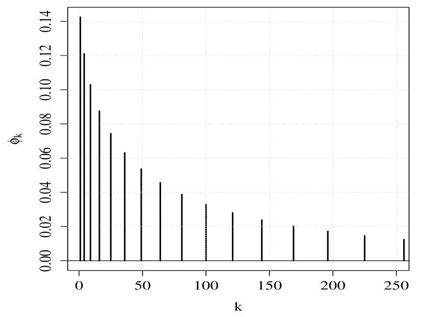
(a) First considered coefficients with corresponding lag.

(b) Sample of three simulated processes.

Figure 1: Considered parameters in 1(a) and simulated sample paths of 3 time series in 1(b) of model (10).

For the estimation the proposed superset ${\mathcal{I}}_{1,1}$ will be important as well. We consider the set ${\mathcal{I}}_{1,1}=\{1,2,\ldots,\lfloor 5\sqrt{n}\rfloor\}$, so we have that $p_{n}\sim\sqrt{n}$.

Subsequently we want evaluate the estimation procedure on the full tuning parameter path. Therefore we estimate (10) for all $\lambda$ values on a given exponential grid $\Lambda=\{2^{g}|g\in{\mathbb{G}}\}$ where ${\mathbb{G}}$ is a equidistant grid from $-4$ to $-18$ of length $100$. Additionally, we want to illustrate the impact of different information criteria. The information criteria that we consider are the Akaike information criterion (AIC), the Hannan-Quinn criterion (HQC) and the Bayesian information criterion (BIC). These are all special cases of the generalised information criterion (see e.g. Kim et al., (2012)) that is given by $\text{GIC}(\kappa_{n})=\log(\widehat{\sigma}_{t}^{2})+\kappa_{n}K/n$, where $K$ represents the number of parameters in the model. We get the AIC, HQC and BIC by choosing either $\kappa_{n}=2$, or $\kappa_{n}=2\log(\log(n))$ or $\kappa_{n}=\log(n)$, respectively. The volatility model is estimated by the methods explained in the section above. The model order is assumed to be known. In all adaptive lasso estimation procedures we choose only the lasso itself, so $\tau=0$. We simulated for $n\in\{300,600,1200\}$ with a Monte Carlo sample size $N=1000$.

After simulating the process, we estimate by the proposed iteratively reweighted lasso algorithm. The first simulation result is given in Figure 2.

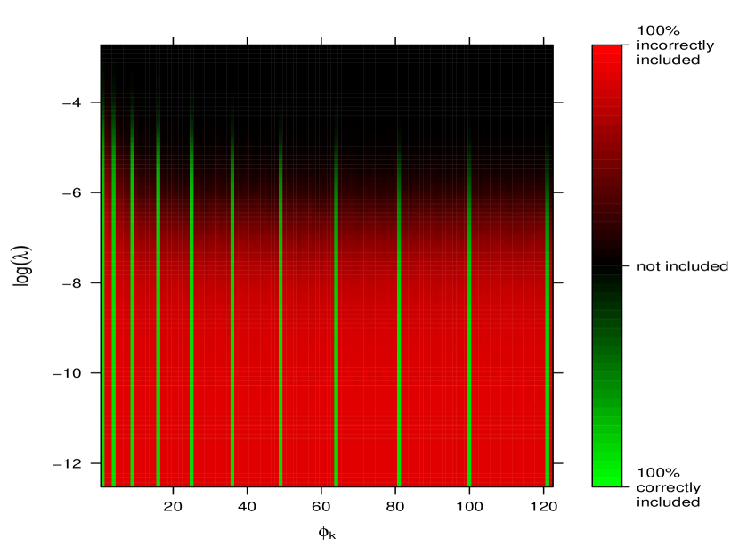
(a) $k=1$

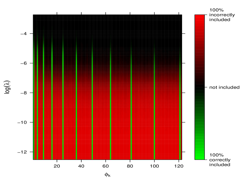
(b) $k=2$

Figure 2: Proportion of irrelevant included parameters (black to red) and relevant included parameters (black to green) for $n=600$ and $\lambda\in\Lambda$.

There we see the proportions of both the irrelevant and relevant included parameters of all estimated parameters for the homoscedastic case ($k=1$) and for the heteroscedastic with one additional replication ($k=2$) given a situation with $n=600$ observations and the exponential grid tuning parameter grid $\Lambda$. Obviously, we observe that for both models the probability to include a parameter increases with decreasing $\lambda$. We see that parameters $\phi_{k}$ with $k\in I_{1,1}$ and small $k$ are easier to detect than those with larger $k$. This is clear as $\phi_{k}$ with $k\in I_{1,1}$ is decreasing in $k$. Further, we can observe that for both cases ($k=1$ and $k=2$) the algorithm seems to distinguish well between relevant parameters and irrelevant parameters. In this situation a reasonable choice of the tuning parameter could be $\log(\lambda)=-6$. There we see that proportion of relevant parameters (green colored) included is clearly closer to 100% than the proportion of irrelevant included parameters (dark red to black). It seems that the heteroscedastic algorithm can distinguish better than its homoscedastic counterpart.

To emphasis this fact we created a new plot where we visualise the computed mean proportion of all irrelevant included parameters against the mean proportion of all relevant included parameters. The mentioned plot is given in Figure 3. We additionally added the corresponding values for the considered information criteria. To understand the impact of the sample size and the number of iterations we plot the cases for $n=600$ and $n=1200$ and the first three iterations of the algorithm.

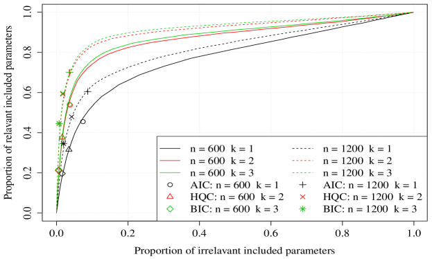
Figure 3: Mean proportion of all irrelevant included parameters against mean proportion of all relevant included parameters for the first three iterations and $n\in\{600,1200\}$ on the full $\lambda$ grid and for the considered information criteria.

The bottom left corner corresponds to very large $\lambda$ values where no parameter at all is included in the model. The top right corner covers the ordinary least square estimate with $\lambda=0$.

Roughly speaking we are aiming for estimators that are as close as possible to the upper left corner. It is particularly important to mention that for increasing $n$ we should get close to the upper left corner. This seems to be satisfied for the relevant tuning parameter path. We see that with the heteroscedastic cases with $k=2$ and $k=3$ have better selection properties than the homoscedastic case. The improvement from the case $k=2$ to $k=3$ is very small, but it is still there. The same holds for the considered information criteria. Note that even though it is well known that the AIC is inconsistent in parameter selection in a finite sample setting it seems to perform quite well.

Nevertheless, it is not clear how the algorithm performs in an out-of-sample forecasting study. Therefore, we conduct another simulation study where we focus on the out-of-sample forecasting error. We compute the $1$-step ahead mean absolute forecast error (MAE) which is defined by $\text{MAE}=\frac{1}{N}\sum_{i=1}^{N}|\widehat{Y}_{n+1}-Y_{n+1}|$ where $\widehat{Y}_{n+1}$ denotes the forecast of $Y_{n+1}$. Additionally, we calculate the forecasting error for the corresponding oracle model. For the oracle we assume that the underlying lag structure of the autoregressive model is known.

The simulation results for $n=300$ and $n=600$ are given in Figure 4.

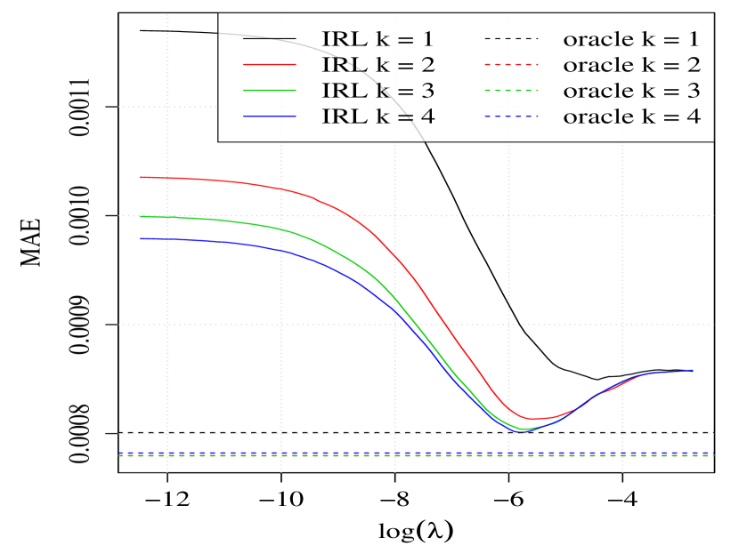
(a) $n=300$

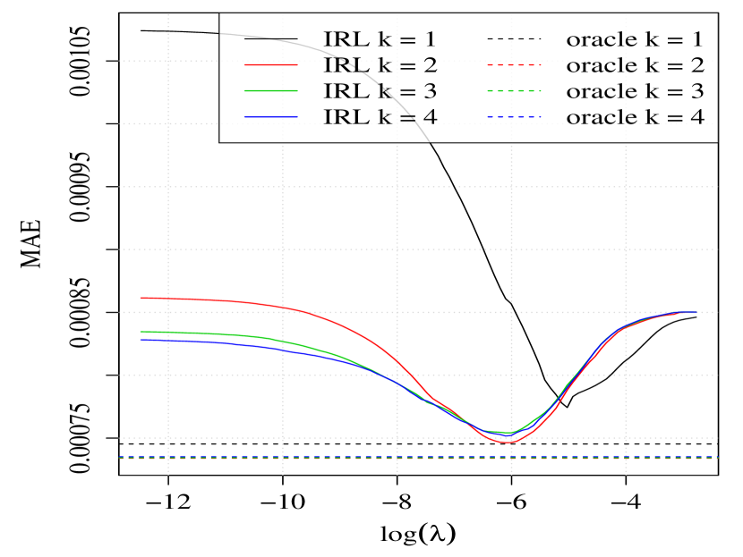
(b) $n=600$

Figure 4: MAE for $n=300$ (4(a)) and $n=600$ (4(b)) of the iteratively reweighted lasso (IRL) method for several iterations $k\in\{1,2,3,4\}$, such as their oracle estimators for the AR-ARCH model.

We see that the homoscedastic algorithm performs significantly worse than the heteroscedastic one with $k=1$, except for large $\lambda$ values in the $n=600$ situation. Interestingly for $n=300$ and $k=1$ the MAE hardly goes below the value of the case with very large $\lambda$ where $\widehat{\phi}_{k}=0$ for all $k\in{\mathcal{I}}_{1,1}$. In contrast for $k>1$ an improvement in the forecasting performance to the case with very large $\lambda$ where $\widehat{\phi}_{k}=0$ is possible. The same fact can be observed, within the oracle procedures, but the improvement is not that obvious. From an applications perspective, this is extremely significant. It indicates that we can benefit more from taking the heteroscedasticity into account in settings with unknown model structure than in a setting where the underlying structure is known. However, we usually do not know the true underlying model as the oracle does, especially in high-dimensional settings. It shows that the proposed estimation algorithm can lead to crucial improvements in a high-dimensional setting. This is also observed by Ziel et al., (2015) in applications of the proposed estimation algorithm to electricity market data.

As a robustness check we replicate the simulation study with a different volatility model. We assume a TARCH process for the residuals. TARCH models are popular in financial applications as they are able to capture leverage effects. The considered TARCH process for the simulation study is parameterised through

$$\sigma_{t}=\alpha_{0}+\alpha_{1}|{\varepsilon}_{t-1}|+\alpha^{-}_{1}\boldsymbol{1}\{{\varepsilon}_{t-1}<0\}|{\varepsilon}_{t-1}|+\alpha_{2}|{\varepsilon}_{t-2}|+\alpha^{-}_{2}\boldsymbol{1}\{{\varepsilon}_{t-2}<0\}|{\varepsilon}_{t-2}|$$

where the leverage effect is modelled by the two parameters $\alpha^{-}_{1}$ and $\alpha^{-}_{2}$ which give an additional impact on negative past residuals to the volatility. The selected parameter setting is $\alpha_{1}=\alpha_{2}=0.245$ and $\alpha^{-}_{1}=\alpha^{-}_{2}=0.49$.

We compute the $1$-step ahead mean absolute forecast error (MAE) for $n=300$ and $n=600$. The simulation results with the corresponding oracles are given in Figure 5.

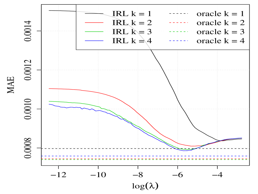
(a) $n=300$

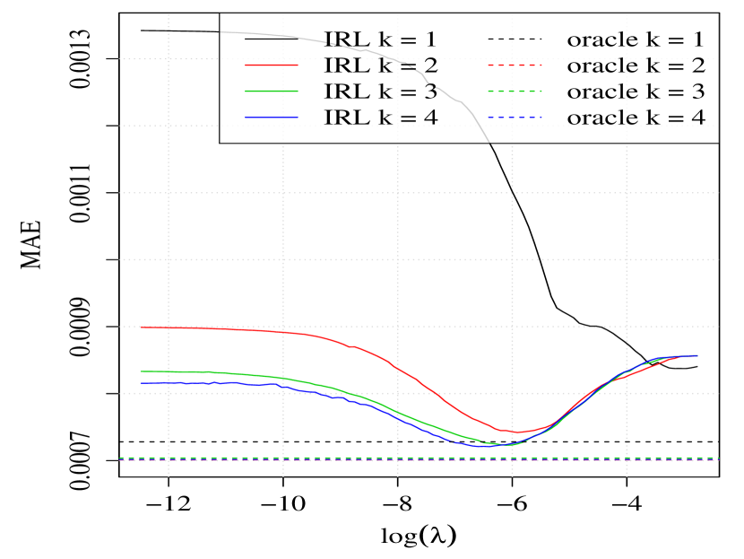
(b) $n=600$

Figure 5: MAE for $n=300$ (5(a)) and $n=600$ (5(b)) of the iteratively reweighted lasso (IRL) method for several iterations $k\in\{1,2,3,4\}$, such as their oracle estimators for the AR-TARCH model.

There we observe similar behaviour as for the AR-ARCH model in Figure 4. As there is a clear improvement in the MAE it shows that the iteratively reweighted lasso algorithm can work well for data with asymmetric volatility.

7 Applications to electricity market data and metal prices returns

In this section we briefly show two applications of the proposed model to real data. For both applications a two-dimensional AR-ARCH model to the process $(\boldsymbol{Y}_{t})_{t\in{\mathbb{Z}}}=(Y_{1,t},Y_{2,t})_{t\in{\mathbb{Z}}}$ is considered.

In the first application we use the hourly day-ahead electricity spot price for Germany/Austria at the European Power exchange (EPEX) as one process $(Y_{1,t})_{t\in{\mathbb{Z}}}$ and the hourly electricity load of Germany as $(Y_{2,t})_{t\in{\mathbb{Z}}}$. The considered time range is from 28.09.2010 to 17.04.2014. For the second example we take the hourly intra-day returns of gold and silver prices in U.S. dollar (from London Bullion Market Association), denoted as XAU/USD and XAG/USD. Here $(Y_{1,t})_{t\in{\mathbb{Z}}}$ represents the gold and $(Y_{2,t})_{t\in{\mathbb{Z}}}$ the silver price returns. The data covers 12 years of observations from 01.01.2002 to 31.12.2013.

Note that electricity prices are known to have a strong correlation structure. In contrast, we expect either no or a very weak autoregressive dependency structure for the commodity returns.

For both applications we suppose that $\boldsymbol{Y}_{t}$ follows an AR-ARCH model as given in (4) and (5). As the electricity data has usually a long memory we propose for the autoregressive parameters the lags ${\mathcal{I}}_{i,j}=\{1,\ldots,700\}$ for $i,j\in\{1,2\}$ and similarly for the ARCH part parameters we take ${\mathcal{J}}_{i,j}=\{1,\ldots,700\}$. This covers a memory of more than 4 weeks. For the metal prices we take ${\mathcal{I}}_{i,j}=\{1,\ldots,200\}$ for the conditional mean and ${\mathcal{J}}_{i,j}=\{1,\ldots,200\}$ for the volatility part. The index sets are sufficiently large to capture possible weekly dependencies. We consider the conservative BIC as information criterion and for the adaption parameter $\tau$ we take the lasso case with $\tau=0$. Then we apply the iteratively reweighted algorithm and stop after $R_{\max}=3$ iterations. Hence we solve $dR_{\max}=2\times 3$ lasso problems in for each application.

The estimated $\widehat{\boldsymbol{\beta}}_{i,n}$ for $i\in\{1,2\}$ and both applications are given in Figure 6.

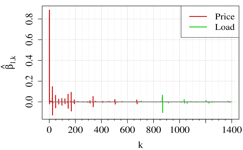
(a) Estimated coefficients for the electricity price

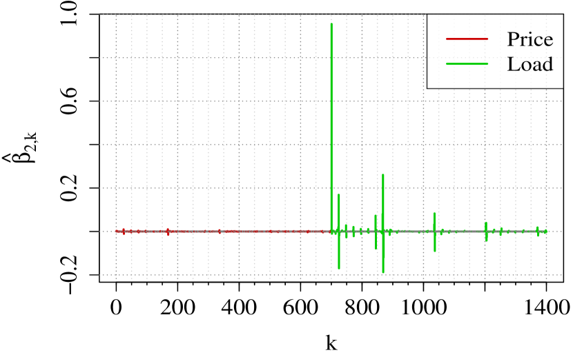
(b) Estimated coefficients for the electricity load

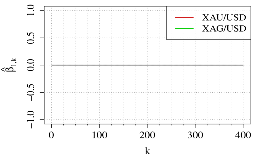
(c) Estimated coefficients for the gold price returns

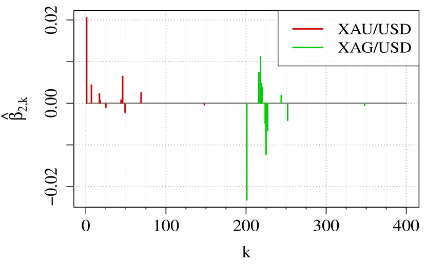
(d) Estimated coefficients for the silver price returns

Figure 6: Estimated parameters $\widehat{\boldsymbol{\beta}}_{i,n}$ for the electricity market model in 6(a) and 6(b) and for the metal prices in 6(c) and 6(d).

Here we see that in general most of the parameters are not included in the model. For the electricity price model there are 133 parameter included and for the load model 416. This matches a proportion of included parameters of $9.5\%$ and $29.7\%$. We see that the complex autocorrelation structure that is driven by daily and weekly seasonal effects is well captured.

For the metal prices we observe a different situation. HHere the gold price returns have no significant parameter at all. However, the silver time series exhibits a weak dependency structure. Most distinct is the first lag pattern with a positive coefficient for the gold returns and a negative one for the silver returns. Furthermore, we have two small silver coefficient clusters, a positive one around a lag of 16 hours and a negative one around a lag of 24.

8 Summary and Conclusion

An iterative algorithm to solve adaptive lasso time series problems with conditionally heteroscedastic residuals is described. We showed the sign consistency and asymptotic normality in a rather general time series setting. The asymptotic theory shows that a significant estimation improvement is possible if the conditional heteroscedasticity is considered. We discussed the application to AR-ARCH type models and showed applications to intra-day electricity market and commodity data.

The simulation studies underline the asymptotic results. Additionally, we showed that considering the heteroscedasticity in high-dimensional settings with unknown parameter specification is more important than in cases where the true underlying model is known, as it can substantially improve forecasting performance. This observation will likely have a strong impact on high-dimensional time series modelling, as almost every time series exhibits conditional heteroscedasticity, especially in economics and finance.

The asymptotic theory shows that only two iterations are required for receiving optimal asymptotic behaviour. Thus, the algorithm is suitable for applications, as the computational effort is only doubled in comparison to standard homoscedastic situations.

For future research it might be important to analyse the mentioned model extensions more carefully. Another very important issue is to identify the optimal penalty parameter $\lambda_{n}$ in high-dimensional time series settings. A different direction of further research might concern the robustness of the algorithm. The performed simulation study carried out that the algorithm works well in a finite sample setting. However, in a heavy tailed situation , it might be worth considering the LAD-lasso (see e.g. Wang et al., 2007a ), which minimises the sum of the absolute residuals, instead of their squares (as in lasso type algorithms). Another direction that seems to be a promising extension concerns the $\ell_{q}$ penalty itself. An extension to elastic net estimators, which combine $\ell_{1}$ and $\ell_{2}$ penalties, could also improve estimation power. Recently Gefang, (2014) applied the elastic net method successfully to homoscedastic multivariate AR processes.

9 Appendix

Proof: Theorem 1.

We show the sign consistency first and then the asymptotic normality. As mentioned, the proof extents mainly methods from Wagener and Dette, (2013). Denote $e_{n,j}$ the $j$’th unit vector in ${\mathbb{R}}^{q_{n}}$, $a=_{s}b$ holds if $\operatorname{sign}(a)=\operatorname{sign}(b)$ and $\|\cdot\|_{\psi_{d}}$ Orlicz norm with ${\psi_{d}}(x)=\exp(x^{d})-1$. In proof we will introduce at some points several constants $c_{k}$ that are positive.

Let $k>1$ and assume that the theorem holds for $k-1$. Following the Karush-Kuhn-Tucker conditions we have that

$$(\boldsymbol{Y}_{n}-\boldsymbol{X}_{n}\boldsymbol{\beta})^{\prime}(\boldsymbol{W}_{n}^{[k-1]})^{2}(\boldsymbol{Y}_{n}-\boldsymbol{X}_{n}\boldsymbol{\beta})+\lambda_{n}\boldsymbol{v}_{n}^{\prime}|\boldsymbol{\beta}|$$

is minimised by $\boldsymbol{\beta}=(\boldsymbol{\beta}(1)^{\prime},\boldsymbol{0}^{\prime})^{\prime}\in{\mathbb{R}}^{p_{n}}$ if and only if

$$X_{j}(1)^{\prime}(\boldsymbol{W}_{n}^{[k-1]})^{2}(\boldsymbol{Y}_{n}-\boldsymbol{X}_{n}\boldsymbol{\beta})=\frac{\lambda_{n}}{2}v_{j}\operatorname{sign}(\beta_{j})\text{ if }\beta_{j}\neq 0\ \ \ \text{ and}$$

$$|X_{j}(1)^{\prime}(\boldsymbol{W}^{[k-1]}_{n})^{2}(\boldsymbol{Y}_{n}-\boldsymbol{X}_{n}\boldsymbol{\beta})|<\frac{\lambda_{n}}{2}v_{j}\text{ if }\beta_{j}=0$$

holds. Thus, we have the estimator $\boldsymbol{\beta}^{[k]}_{n}=(\boldsymbol{\beta}^{[k]}_{n}(1)^{\prime},\boldsymbol{0}^{\prime})^{\prime}\in{\mathbb{R}}^{p_{n}}$ where

$$\boldsymbol{\beta}^{[k]}_{n}(1)=\boldsymbol{\beta}_{n}^{0}(1)+\frac{1}{n}(\widetilde{\boldsymbol{\Gamma}}_{n}^{[k]}(1))^{-1}\boldsymbol{X}_{n}(1)(\boldsymbol{W}_{n}^{[k-1]})^{2}\boldsymbol{\varepsilon}_{n}^{0}-\frac{\lambda_{n}}{2n}(\widetilde{\boldsymbol{\Gamma}}_{n}^{[k]}(1))^{-1}\boldsymbol{s}^{0}_{n}(1)$$ (11)

where $\boldsymbol{s}^{0}_{n}(1)=(v_{1},\ldots,v_{q_{n}})^{\prime}\operatorname{sign}(\boldsymbol{\beta}_{n}^{0}(1))$.

Now we define the expressions

$$\eta_{1,j} =e_{n,j}^{\prime}(\widetilde{\boldsymbol{\Gamma}}_{n}^{[k]}(1))^{-1}\boldsymbol{X}_{n}(1)^{\prime}(\boldsymbol{W}_{n}^{[k-1]})^{2}\boldsymbol{\varepsilon}_{n}^{0}$$

$$\eta_{2,j} =e_{n,j}^{\prime}(\widetilde{\boldsymbol{\Gamma}}_{n}^{[k]}(1))^{-1}\boldsymbol{s}^{0}_{n}(1)$$

$$\eta_{3,j} =X_{j}(1)^{\prime}(\boldsymbol{W}_{n}^{[k-1]})^{2}(I_{n}-n^{-1}\boldsymbol{X}_{n}(1)(\widetilde{\boldsymbol{\Gamma}}_{n}^{[k]}(1))^{-1}\boldsymbol{X}_{n}(1)^{\prime}(\boldsymbol{W}_{n}^{[k-1]})^{2})\boldsymbol{\varepsilon}_{n}^{0}$$

$$\eta_{4,j} =\lambda_{n}(2n)^{-1}X_{j}(1)^{\prime}(\boldsymbol{W}_{n}^{[k-1]})^{2}\boldsymbol{X}_{n}(1)(\widetilde{\boldsymbol{\Gamma}}_{n}^{[k]}(1))^{-1}\boldsymbol{s}^{0}_{n}(1).$$

As in Wagener and Dette, (2013) we can use the argument of Huang et al., (2008) that the KKT conditions are satisfied if

$$|\eta_{3,j}-\eta_{4,j}|<\frac{\lambda_{n}}{2}v_{j}$$ (12)

holds for all $j>q_{n}$.

Hence we receive with (11) and (12) that

$$P\left(\boldsymbol{\beta}_{n}^{[k]}\neq_{s}\boldsymbol{\beta}_{n}^{0}\right)\leq P(A_{1})+P(A_{2})+P(A_{3})+P(A_{4}),\ \ \ \text{ with}$$

$$A_{1} =\left\{\frac{1}{n}|\eta_{1,j}|\geq\frac{1}{2}|\beta^{0}_{j}|\text{ for some }j\leq q_{n}\right\},\ \ \ A_{2}=\left\{\frac{\lambda_{n}}{n}|\eta_{2,j}|\geq|\beta^{0}_{j}|\text{ for some }j\leq q_{n}\right\},$$

$$A_{3} =\left\{|\eta_{3,j}|\geq\frac{\lambda_{n}}{4}v_{j}\text{ for some }j>q_{n}\right\}\ \text{ and }A_{4}=\left\{|\eta_{4,j}|\geq\frac{\lambda_{n}}{4}v_{j}\text{ for some }j>q_{n}\right\}.$$

So we only need to show that $P(A_{j})\to 0$ as $n\to\infty$.

Regarding $P(A_{1})$ we have with definition of $b_{n}$ (see (d)) that

$$P(A_{1}) \leq P\left(\frac{1}{n}\max_{1\leq j\leq q_{n}}|\eta_{1,j}|\geq\frac{b_{n}}{2}\right)$$

$$\leq P\left(\frac{1}{n}\max_{1\leq j\leq q_{n}}|\eta^{0,\infty}_{1,j}|\geq\frac{b_{n}}{4}\right)+P\left(\frac{1}{n}\max_{1\leq j\leq q_{n}}|\eta_{1,j}-\eta^{0}_{1,j}|\geq\frac{b_{n}}{8}\right)+P\left(\frac{1}{n}\max_{1\leq j\leq q_{n}}|\eta^{0}_{1,j}-\eta^{0,\infty}_{1,j}|\geq\frac{b_{n}}{8}\right)$$ (13)

where $\eta^{0}_{1,j}=e_{n,j}^{\prime}(\widetilde{\boldsymbol{\Gamma}}_{n}^{0}(1))^{-1}\boldsymbol{X}_{n}(1)^{\prime}(\boldsymbol{W}_{n}^{0})^{2}\boldsymbol{\varepsilon}^{0}_{n}$ and $\eta^{0,\infty}_{1,j}=e_{n,j}^{\prime}(\widetilde{\boldsymbol{\Gamma}}_{n}^{0}(1))^{-1}\boldsymbol{X}_{n}(1)^{\prime}(\boldsymbol{W}_{n}^{0})^{2}\boldsymbol{\varepsilon}^{0}_{n,\infty}$.

For estimating the first term in (13) we observe that

$$\left\|\frac{1}{\sqrt{n}}e_{n,j}^{\prime}(\widetilde{\boldsymbol{\Gamma}}_{n}^{0}(1))^{-1}\boldsymbol{X}_{n}(1)^{\prime}(\boldsymbol{W}_{n}^{0})^{2}\right\|_{2} \leq\left\|(\widetilde{\boldsymbol{\Gamma}}^{0}_{n}(1))^{-1}\right\|_{2}\left\|\frac{1}{\sqrt{n}}\boldsymbol{X}_{n}(1)^{\prime}\right\|_{2}\|\boldsymbol{W}_{n}^{0}\|^{2}_{2}$$

$$\leq\left\|(\widetilde{\boldsymbol{\Gamma}}^{0}_{n}(1))^{-1}\right\|_{2}\left\|\boldsymbol{\Gamma}^{0}_{n}(1)\right\|_{2}^{\frac{1}{2}}\left\|\boldsymbol{W}_{n}^{0}\right\|^{2}_{2}\leq\left\|(\widetilde{\boldsymbol{\Gamma}}^{0}_{n}(1))^{-1}\right\|_{2}\left\|\boldsymbol{\Gamma}^{0}_{n}(1)\right\|_{2}^{\frac{1}{2}}\sigma^{2}_{\min}$$

for sufficiently large $n$ with $\|\boldsymbol{W}_{n}^{0}\|_{2}\leq\sigma_{\min}$ by (g). Furthermore by assumption (f) we know that

$$\|\boldsymbol{\Gamma}_{n}^{0}(1)\|^{\frac{1}{2}}_{2}={\mathcal{O}}_{P}(1)\ \text{ and }\ \|(\widetilde{\boldsymbol{\Gamma}}_{n}^{0}(1))^{-1}\|_{2}={\mathcal{O}}_{P}(1).$$ (14)

Thus we get that

$$P\left(\left\|e_{n,j}^{\prime}(\widetilde{\boldsymbol{\Gamma}}_{n}^{0}(1))^{-1}\boldsymbol{X}_{n}(1)^{\prime}(\boldsymbol{W}_{n}^{0})^{2}\right\|_{2}\leq\lambda_{1,\min}^{-1}\sqrt{\lambda_{0,\max}}\sigma_{\min}\right)\to 1$$

for $n\to\infty$. With Lemma 1 (i) of Huang et al., (2006) and tail assumption (k) we can deduce that

$$\left\|\frac{1}{\sqrt{n}}\eta_{1,j}^{0,\infty}\right\|_{\psi_{d}}\leq\left\|\frac{1}{\sqrt{n}}e_{n,j}^{\prime}(\widetilde{\boldsymbol{\Gamma}}_{n}^{0}(1))^{-1}\boldsymbol{X}_{n}(1)^{\prime}(\boldsymbol{W}_{n}^{0})^{2}\boldsymbol{\varepsilon}_{\infty,n}^{0}\right\|_{\psi_{d}}\leq c_{1}\log(n)^{\boldsymbol{1}\{d=1\}}$$ (15)

for sufficiently large $n$, as $\|X\|_{2}\leq c\|X\|_{\psi_{d}}$ for some $c>0$.

Thus, we can conclude with Markov inequality, Lemma 2.2.2 of Van der Vaart and Wellner, (1996) and (15) that

$$P\left(\frac{1}{n}\max_{1\leq j\leq q_{n}}|\eta^{0,\infty}_{1,j}|\geq\frac{b_{n}}{4}\right) \leq P\left(\psi_{d}\left(\frac{\max_{1\leq j\leq q_{n}}|\eta^{0,\infty}_{1,j}|}{\|\max_{1\leq j\leq q_{n}}|\eta^{0,\infty}_{1,j}|\|_{\psi_{d}}}\right)\geq\psi_{d}\left(\frac{b_{n}n}{4\|\max_{1\leq j\leq q_{n}}|\eta^{0,\infty}_{1,j}|\|_{\psi_{d}}}\right)\right)$$

$$\leq\psi_{d}\left(\frac{b_{n}n}{4\|\max_{1\leq j\leq q_{n}}|\eta^{0,\infty}_{1,j}|\|_{\psi_{d}}}\right)^{-1}$$

$$\leq\psi_{d}\left(\frac{b_{n}n}{4c_{2}{\psi_{d}}^{-1}(q_{n})\max_{1\leq j\leq q_{n}}\|\eta^{0,\infty}_{1,j}\|_{\psi_{d}}}\right)^{-1}$$

$$\leq\psi_{d}\left(\frac{b_{n}\sqrt{n}}{4c_{2}\log(1+q_{n})^{\frac{1}{d}}c_{2}\log(n)^{\boldsymbol{1}\{d=1\}}}\right)^{-1}$$ (16)

as $\psi_{d}^{-1}(x)=\log(1+x)^{\frac{1}{d}}$. Hence by assumption (j) we have $P\left(\frac{1}{n}\max_{1\leq j\leq q_{n}}|\eta^{0,\infty}_{1,j}|\geq\frac{b_{n}}{4}\right)\to 0$.

If assumption (k) is not satisfied we can not use equation (15) to derive that $P\left(\frac{1}{n}\max_{1\leq j\leq q_{n}}|\eta^{0,\infty}_{1,j}|\geq\frac{b_{n}}{4}\right)\to 0$. But we can conclude with Chebyshev’s inequality and (33) shown below that

$$P\left(\frac{1}{n}\max_{1\leq j\leq q_{n}}|\eta^{0,\infty}_{1,j}|\geq\frac{b_{n}}{4}\right) \leq\frac{16}{n^{2}b_{n}^{2}}{\mathbb{E}}(\max_{1\leq j\leq q_{n}}|\eta^{0,\infty}_{1,j}|^{2})={\mathcal{O}}_{P}\left(\frac{1}{nb_{n}^{2}}\right).$$

Thus even without assumption (k) it holds with assumption (j) that $P\left(\frac{1}{n}\max_{1\leq j\leq q_{n}}|\eta^{0,\infty}_{1,j}|\geq\frac{b_{n}}{4}\right)\to 0$. However, note that either (k) or (k’) is required for estimating the probability of $A_{3}$ in a similar situation.

For the second term in (13) we proceed as in Wagener and Dette, (2013). We get

$$|\eta_{1,j}-\eta^{0}_{1,j}|\leq \left|e_{j,n}^{\prime}\left((\widetilde{\boldsymbol{\Gamma}}_{n}^{0}(1))^{-1}\boldsymbol{X}_{n}(1)^{\prime}((\boldsymbol{W}_{n}^{0})^{2}-(\boldsymbol{W}_{n}^{[k-1]})^{2})+(\widetilde{\boldsymbol{\Gamma}}_{n}^{0}(1)-\widetilde{\boldsymbol{\Gamma}}_{n}^{[k]}(1))\boldsymbol{X}_{n}(1)^{\prime}(\boldsymbol{W}_{n}^{[k-1]})^{2}\right)\boldsymbol{\varepsilon}_{n}^{0}\right|$$

$$\leq \|((\boldsymbol{W}_{n}^{0})^{2}-(\boldsymbol{W}_{n}^{[k-1]})^{2})\boldsymbol{X}_{n}(1)(\widetilde{\boldsymbol{\Gamma}}_{n}^{0}(1))^{-1}e_{j,n}\|_{2}\|\boldsymbol{\varepsilon}_{n}^{0}\|_{2}+\|(\boldsymbol{W}_{n}^{[k-1]})^{2}\boldsymbol{X}_{n}(1)\|_{2}\|\boldsymbol{\varepsilon}_{n}^{0}(\widetilde{\boldsymbol{\Gamma}}_{n}^{0}(1)-\widetilde{\boldsymbol{\Gamma}}_{n}^{[k]}(1))\|_{2}$$

$$\leq \|(\boldsymbol{W}_{n}^{0})^{2}-(\boldsymbol{W}_{n}^{[k-1]})^{2}\|_{2}\|n\boldsymbol{\Gamma}_{n}^{0}(1)\|^{\frac{1}{2}}_{2}\|(\widetilde{\boldsymbol{\Gamma}}_{n}^{0}(1))^{-1}\|_{2}\|\boldsymbol{\varepsilon}_{n}^{0}\|_{2}$$

$$+\|(\boldsymbol{W}_{n}^{0})^{2}\|_{2}\|n\boldsymbol{\Gamma}_{n}^{0}(1)\|^{\frac{1}{2}}_{2}\|(\widetilde{\boldsymbol{\Gamma}}_{n}^{0}(1))^{-1}-(\widetilde{\boldsymbol{\Gamma}}_{n}^{[k]}(1))^{-1}\|_{2}\|\boldsymbol{\varepsilon}_{n}^{0}\|_{2}.$$ (17)

All these appearing single norms we will estimate now.

For the estimation of $\|(\boldsymbol{W}_{n}^{0})^{2}-(\boldsymbol{W}_{n}^{[k-1]})^{2}\|_{2}$ we get directly with assumption (g), (h) and (i) that

$$\|(\boldsymbol{W}_{n}^{0})^{2}-(\boldsymbol{W}_{n}^{[k-1]})^{2}\|_{2}={\mathcal{O}}_{P}\left(\frac{h_{n}}{\sqrt{n}}\right).$$ (18)

For estimating $\|\boldsymbol{\varepsilon}_{n}^{0}\|_{2}$ the triangle inequality yields $\|\boldsymbol{\varepsilon}_{n}^{0}\|_{2}\leq\|\boldsymbol{\varepsilon}_{n}^{0}-\boldsymbol{\varepsilon}_{\infty,n}^{0}\|_{2}+\|\boldsymbol{\varepsilon}_{\infty,n}^{0}\|_{2}$. We have

$$\|\boldsymbol{\varepsilon}_{n}^{0}-\boldsymbol{\varepsilon}_{\infty,n}^{0}\|_{2}=\bigg{\|}\sum_{j=p_{n}+1}^{\infty}\beta_{k}X_{i,k}\bigg{\|}_{2}\to 0$$ (19)

as $\sum_{j=p_{n}+1}^{\infty}|\beta_{k}|<\infty$ and $\|\boldsymbol{\varepsilon}_{\infty,n}^{0}\|={\mathcal{O}}_{P}(\sqrt{n})$ by law of large numbers. Thus we get

$$\|\boldsymbol{\varepsilon}_{n}^{0}\|_{2}={\mathcal{O}}_{P}(\sqrt{n}).$$ (20)

Further we have $\|\boldsymbol{W}_{n}^{[k-1]}\|_{2}={\mathcal{O}}_{P}(1)$ by assumption (g).

Next, we have as in Wagener and Dette, (2013) that with assumption (f), and equations (14) and (18) that

$$\|\widetilde{\boldsymbol{\Gamma}}_{n}^{0}(1)-\widetilde{\boldsymbol{\Gamma}}_{n}^{[k]}(1)\|_{2}\leq\|\boldsymbol{\Gamma}_{n}(1)\|_{2}\|(\boldsymbol{W}_{n}^{0})^{2}-(\boldsymbol{W}_{n}^{[k-1]})^{2}\|_{2}={\mathcal{O}}_{P}\left(\frac{h_{n}}{\sqrt{n}}\right).$$

This leads to

$$\|(\widetilde{\boldsymbol{\Gamma}}_{n}^{0})^{-1}-(\widetilde{\boldsymbol{\Gamma}}_{n}^{[k]})^{-1}\|_{2}={\mathcal{O}}_{P}\left(\frac{h_{n}}{\sqrt{n}}\right)$$ (21)

by using the the triangle inequality

$$\|A^{-1}-(A+B)^{-1}\|_{2}\leq\|A^{-1}-(A+B)^{-1}+A^{-1}BA^{-1}\|_{2}+\|A^{-1}BA^{-1}\|_{2}\leq{\mathcal{O}}_{P}(\|B\|_{2})+\|A\|^{2}_{2}\|B\|_{2}={\mathcal{O}}_{P}\left(\frac{h_{n}}{\sqrt{n}}\right)$$

for two matrices $A=\widetilde{\boldsymbol{\Gamma}}_{n}^{0}(1)$ with $B=\widetilde{\boldsymbol{\Gamma}}_{n}^{0}(1)-\widetilde{\boldsymbol{\Gamma}}_{n}^{[k]}(1)$ and the Taylor series expansion of $(A+B)^{-1}$ around $A^{-1}$.

Using all the estimated norms ((14), (18), (20) and (21)) we receive for (17) that

$$|\eta_{1,j}-\eta^{0}_{1,j}|\leq \|(\boldsymbol{W}_{n}^{0})^{2}-(\boldsymbol{W}_{n}^{[k-1]})^{2}\|_{2}\|n\boldsymbol{\Gamma}_{n}^{0}(1)\|^{\frac{1}{2}}_{2}\|(\widetilde{\boldsymbol{\Gamma}}_{n}^{0}(1))^{-1}\|_{2}\|\boldsymbol{\varepsilon}_{n}^{0}\|_{2}$$

$$+\|(\boldsymbol{W}_{n}^{0})^{2}\|_{2}\|n\boldsymbol{\Gamma}_{n}^{0}(1)\|^{\frac{1}{2}}_{2}\|(\widetilde{\boldsymbol{\Gamma}}_{n}^{0}(1))^{-1}-(\widetilde{\boldsymbol{\Gamma}}_{n}^{[k]}(1))^{-1}\|_{2}\|\boldsymbol{\varepsilon}_{n}^{0}\|_{2}$$

$$\leq {\mathcal{O}}_{P}(\frac{h_{n}}{\sqrt{n}}){\mathcal{O}}_{P}(\sqrt{n}){\mathcal{O}}_{P}(1){\mathcal{O}}_{P}(\sqrt{n})+{\mathcal{O}}_{P}(1){\mathcal{O}}_{P}(\sqrt{n}){\mathcal{O}}_{P}(\frac{h_{n}}{\sqrt{n}}){\mathcal{O}}_{P}(\sqrt{n})={\mathcal{O}}_{P}(h_{n}\sqrt{n}).$$

Thus we get,

$$\frac{1}{n}\max_{1\leq j\leq q_{n}}|\eta_{1,j}-\eta^{0}_{1,j}|=\frac{1}{n}{\mathcal{O}}_{P}(h_{n}\sqrt{n})={\mathcal{O}}_{P}\left(\frac{h_{n}}{\sqrt{n}}\right).$$

This yields with assumption (j) that $P\left(\frac{1}{n}\max_{1\leq j\leq q_{n}}|\eta_{1,j}-\eta^{0}_{1,j}|\geq\frac{b_{n}}{8}\right)\to 0$ as $n\to\infty$. For the third term in (13) we get with (g), (14) and (19) that

$$\frac{1}{\sqrt{n}}|\eta^{0}_{1,j}-\eta^{0,\infty}_{1,j}| \leq\frac{1}{\sqrt{n}}|e_{n,j}^{\prime}(\widetilde{\boldsymbol{\Gamma}}_{n}^{0}(1))^{-1}\boldsymbol{X}_{n}(1)^{\prime}(\boldsymbol{W}_{n}^{0})^{2}(\boldsymbol{\varepsilon}_{n}^{0}-\boldsymbol{\varepsilon}_{n,\infty}^{0})|$$

$$\leq\|(\widetilde{\boldsymbol{\Gamma}}_{n}^{0}(1))^{-1}\|_{2}\left\|\frac{1}{\sqrt{n}}\boldsymbol{X}_{n}(1)^{\prime}\right\|_{2}\|\boldsymbol{W}_{n}^{0}\|^{2}_{2}\|\boldsymbol{\varepsilon}_{n}^{0}-\boldsymbol{\varepsilon}_{n,\infty}^{0}\|_{2}$$

$$\leq\|(\widetilde{\boldsymbol{\Gamma}}_{n}^{0}(1))^{-1}\|_{2}\left\|\boldsymbol{\Gamma}_{n}^{0}\right\|_{2}^{\frac{1}{2}}\|\boldsymbol{W}_{n}^{0}\|^{2}_{2}\|\boldsymbol{\varepsilon}_{n}^{0}-\boldsymbol{\varepsilon}_{n,\infty}^{0}\|_{2}\to 0$$

as $n\to\infty$. So we have that $\frac{1}{n}|\eta^{0}_{1,j}-\eta^{0,\infty}_{1,j}|\to\infty$ as $n\to 0$. This implies $P(A_{1})\to 0$.

Now we consider $P(A_{2})\leq P(\frac{\lambda_{n}}{n}\max_{1\leq j\leq q_{n}}|\eta_{2,j}|\geq b_{n})$. We have $|\eta_{2,j}|\leq\|(\widetilde{\boldsymbol{\Gamma}}_{n}^{[k]})^{-1}\|_{2}\|\boldsymbol{s}^{0}_{n}(1)\|_{2}$ for each $j\in\{1,\ldots,q_{n}\}$. By Weyl’s perturbation theorem for the matrices $(\widetilde{\boldsymbol{\Gamma}}_{n}^{0}(1))^{-1}$ and $(\widetilde{\boldsymbol{\Gamma}}_{n}^{[k]}(1))^{-1}$ we have for each ordered pair of eigenvalues that

$$\left|\lambda_{j}\left((\widetilde{\boldsymbol{\Gamma}}_{n}^{0}(1))^{-1}\right)-\lambda_{j}\left((\widetilde{\boldsymbol{\Gamma}}_{n}^{[k]}(1))^{-1}\right)\right|\leq\|(\widetilde{\boldsymbol{\Gamma}}_{n}^{0}(1))^{-1}-(\widetilde{\boldsymbol{\Gamma}}_{n}^{[k]}(1))^{-1}\|_{2}$$

for each $j\in\{1,\ldots,q_{n}\}$. As $\|(\widetilde{\boldsymbol{\Gamma}}_{n}^{0}(1))^{-1}-(\widetilde{\boldsymbol{\Gamma}}_{n}^{[k]}(1))^{-1}\|_{2}\to 0$ in probability, we get with (f) that

$$\|(\widetilde{\boldsymbol{\Gamma}}_{n}^{[k]})^{-1}\|_{2}\leq\lambda_{1,\min}^{-1}+c_{3}$$ (22)

with probability arbitrarily close to 1 for sufficiently large $n$.

Furthermore, with assumption (d) we have

$$\|\boldsymbol{s}^{0}_{n}(1)\|_{2}\leq\sqrt{q_{n}}\sqrt{\max_{1\leq j\leq q_{n}}|\beta_{\text{init},j}|^{-\tau}}\leq\frac{\sqrt{bq_{n}}}{\sqrt{b_{n}}}.$$ (23)

Hence we have with assumption (j) that $\leq P\left(\frac{\lambda_{n}}{n}\max_{1\leq j\leq q_{n}}|\eta_{2,j}|\geq b_{n}\right)\leq P\left(\frac{\lambda_{n}}{n}c_{4}\frac{\sqrt{bq_{n}}}{\sqrt{b_{n}}}\geq b_{n}\right)\to 0$ as $n\to\infty$.

For $A_{3}$ we receive similarly as for $A_{1}$ that

$$P(A_{3})\leq P\left(\max_{q_{n}<j\leq p_{n}}|\eta_{3,j}^{0,\infty}|\geq\frac{\lambda_{n}r_{n}}{8}\right)+P\left(\max_{q_{n}<j\leq p_{n}}|\eta_{3,j}^{0}-\eta_{3,j}^{0,\infty}|\geq\frac{\lambda_{n}r_{n}}{16}\right)$$

$$+P\left(\max_{q_{n}<j\leq p_{n}}|\eta_{3,j}-\eta_{3,j}^{0}|\geq\frac{\lambda_{n}r_{n}}{16}\right)+P\left(\max_{q_{n}<j\leq p_{n}}\boldsymbol{\beta}_{j,\text{init}}^{\tau}>r_{n}^{-1}\right)$$ (24)

where

$$\eta_{3,j}^{0} =X_{j}(1)^{\prime}(\boldsymbol{W}_{n}^{0})^{2}(I_{n}-n^{-1}\boldsymbol{X}_{n}(1)(\widetilde{\boldsymbol{\Gamma}}_{n}^{0})^{-1}\boldsymbol{X}_{n}(1)^{\prime}(\boldsymbol{W}_{n}^{0})^{2})\boldsymbol{\varepsilon}_{n}^{0},$$

$$\eta_{3,j}^{0,\infty} =X_{j}(1)^{\prime}(\boldsymbol{W}_{n}^{0})^{2}(I_{n}-n^{-1}\boldsymbol{X}_{n}(1)(\widetilde{\boldsymbol{\Gamma}}_{n}^{0})^{-1}\boldsymbol{X}_{n}(1)^{\prime}(\boldsymbol{W}_{n}^{0})^{2})\boldsymbol{\varepsilon}_{n,\infty}^{0}.$$

As in Wagener and Dette, (2013) we consider $\eta_{3,j}^{0,\infty}=H_{n,j}^{0}\boldsymbol{\varepsilon}_{n,\infty}^{0}$ with

$$H_{n,j}^{0}=X_{j}(1)^{\prime}(\boldsymbol{W}_{n}^{0})^{2}(I_{n}-n^{-1}\boldsymbol{X}_{n}(1)(\widetilde{\boldsymbol{\Gamma}}_{n}^{0})^{-1}\boldsymbol{X}_{n}(1)^{\prime}(\boldsymbol{W}_{n}^{0})^{2}).$$

Then we have for sufficiently large $n$ that

$$\|H_{n,j}^{0}\|_{2} \leq\|X_{j}(1)^{\prime}\|_{2}\|(\boldsymbol{W}_{n}^{0})^{2}\|_{2}(1+\|n^{-1}\boldsymbol{X}_{n}(1)(\widetilde{\boldsymbol{\Gamma}}_{n}^{0})^{-1}\boldsymbol{X}_{n}(1)^{\prime}\|_{2}\|(\boldsymbol{W}_{n}^{0})^{2}\|_{2})$$

$$={\mathcal{O}}_{P}(\sqrt{n}){\mathcal{O}}_{P}(1)(1+{\mathcal{O}}_{P}(1){\mathcal{O}}_{P}(1))={\mathcal{O}}_{P}(\sqrt{n}).$$ (25)

Now we receive we receive as in equation (15) with Huang et al., (2006) Lemma 1 (i) and assumption (k) that

$$\left\|\frac{1}{\sqrt{n}}\eta_{3,j}^{0,\infty}\right\|_{\psi_{d}}\leq\left\|\frac{1}{\sqrt{n}}H_{n,j}^{0}\boldsymbol{\varepsilon}_{\infty,n}^{0}\right\|_{\psi_{d}}\leq c_{6}\log(n)^{\boldsymbol{1}{\{d=1\}}}.$$ (26)

Thus we get with Markov inequality, Lemma 2.2.2 of Van der Vaart and Wellner, (1996), (26) and assumption (j) similarly to (16) that

$$P\left(\max_{q_{n}<j\leq p_{n}}|\eta_{3,j}^{0,\infty}|\geq\frac{\lambda_{n}r_{n}}{8}\right)\leq \psi_{d}\left(\frac{\lambda_{n}r_{n}}{8c_{6}\psi_{d}^{-1}(q_{n})\max_{q_{n}<j\leq p_{n}}\|\eta_{3,j}^{0}\|_{\psi_{d}}}\right)^{-1}$$

$$\leq \psi_{d}\left(\frac{\lambda_{n}r_{n}}{c_{7}\sqrt{n}\log(1+p_{n}-q_{n})^{\frac{1}{d}}\log(n)^{\boldsymbol{1}{\{d=1\}}}}\right)^{-1}\to 0$$ (27)

as $n\to\infty$.

If instead of (k) the alternative assumption (k’) holds we can not use equation (26) to derive that it holds $P\left(\max_{q_{n}<j\leq p_{n}}|\eta^{0,\infty}_{3,j}|\geq\frac{\lambda_{n}r_{n}}{8}\right)\to 0$. But can get with Chebyshev’s inequality and (33) shown below that

$$P\left(\max_{q_{n}<j\leq p_{n}}|\eta^{0,\infty}_{3,j}|\geq\frac{\lambda_{n}r_{n}}{8}\right) \leq\frac{64}{\lambda_{n}r_{n}^{2}}\sum_{j=q_{n}+1}^{p_{n}}{\mathbb{E}}(|\eta^{0,\infty}_{3,j}|^{2})={\mathcal{O}}_{P}\left(\frac{n(p_{n}-q_{n})}{\lambda_{n}^{2}r_{n}^{2}}\right).$$

Thus with (k’) it holds $P\left(\max_{q_{n}<j\leq p_{n}}|\eta^{0,\infty}_{1,j}|\geq\frac{\lambda_{n}^{2}r_{n}}{8}\right)\to 0$.

For estimating the second term in (24) we note with (19) and (25) that

$$\frac{1}{\sqrt{n}}\left|\eta_{3,j}^{0}-\eta_{3,j}^{0,\infty}\right|\leq\left|\frac{1}{\sqrt{n}}H_{n,j}^{0}(\boldsymbol{\varepsilon}_{n}^{0}-\boldsymbol{\varepsilon}_{\infty,n}^{0})\right|\leq\frac{c_{8}}{\sqrt{n}}\left\|H_{n,j}^{0}\|_{2}\|\boldsymbol{\varepsilon}_{n}^{0}-\boldsymbol{\varepsilon}_{\infty,n}^{0}\right\|_{2}=\frac{1}{\sqrt{n}}{\mathcal{O}}_{P}(\sqrt{n}).$$

Hence we have with assumption (j) that

$$P\left(\max_{q_{n}<j\leq p_{n}}|\eta_{3,j}^{0}-\eta_{3,j}^{0,\infty}|\geq\frac{\lambda_{n}r_{n}}{16}\right)\leq P\left(\frac{\sqrt{n}}{\lambda_{n}r_{n}}\geq c_{9}\right)\to 0$$ (28)

as $n\to\infty$. Now we estimate the third term in (24). As in (17) we get the estimate

$$|\eta_{3,j}^{0}-\eta_{3,j}|\leq \left|X_{j}(1)^{\prime}\left((\boldsymbol{W}_{n}^{0})^{2}(I_{n}-n^{-1}\boldsymbol{X}_{n}(1)(\widetilde{\boldsymbol{\Gamma}}_{n}^{0})^{-1}\boldsymbol{X}_{n}(1)^{\prime}(\boldsymbol{W}_{n}^{0})^{2})\right.\right.$$

$$-\left.\left.(\boldsymbol{W}_{n}^{[k-1]})^{2}(I_{n}-n^{-1}\boldsymbol{X}_{n}(1)(\widetilde{\boldsymbol{\Gamma}}_{n}^{[k]})^{-1}\boldsymbol{X}_{n}(1)^{\prime}(\boldsymbol{W}_{n}^{[k-1]})^{2}\right)\boldsymbol{\varepsilon}_{n}^{0}\right|$$

$$\leq \|X_{j}(1)\|_{2}\|(\boldsymbol{W}_{n}^{0})^{2}-(\boldsymbol{W}_{n}^{[k-1]})^{2}\|_{2}\|\boldsymbol{\varepsilon}_{n}^{0}\|_{2}$$ (29)

$$+\|X_{j}(1)\|_{2}\left\|n^{-1}\left(\boldsymbol{X}_{n}(1)(\widetilde{\boldsymbol{\Gamma}}_{n}^{0})^{-1}\boldsymbol{X}_{n}(1)^{\prime}(\boldsymbol{W}_{n}^{0})^{2}-\boldsymbol{X}_{n}(1)(\widetilde{\boldsymbol{\Gamma}}_{n}^{[k]})^{-1}\boldsymbol{X}_{n}(1)^{\prime}(\boldsymbol{W}_{n}^{[k-1]})^{2}\right)\right\|_{2}\|\boldsymbol{\varepsilon}_{n}^{0}\|_{2}$$

using estimates derived for $A_{1}$. For the lengthy norm in (29) we get

$$\left\|n^{-1}\left(\boldsymbol{X}_{n}(1)(\widetilde{\boldsymbol{\Gamma}}_{n}^{0})^{-1}\boldsymbol{X}_{n}(1)^{\prime}(\boldsymbol{W}_{n}^{0})^{2}-\boldsymbol{X}_{n}(1)(\widetilde{\boldsymbol{\Gamma}}_{n}^{[k]})^{-1}\boldsymbol{X}_{n}(1)^{\prime}(\boldsymbol{W}_{n}^{[k-1]})^{2}\right)\right\|_{2}$$

$$\leq \|(\boldsymbol{W}_{n}^{0})^{2}-(\boldsymbol{W}_{n}^{[k-1]})^{2}\|_{2}\|\boldsymbol{\Gamma}_{n}(1)\|_{2}\|(\widetilde{\boldsymbol{\Gamma}}_{n}^{[k]})^{-1}\|_{2}\|(\boldsymbol{W}_{n}^{[k-1]})^{2}\|_{2}$$

$$+\|(\widetilde{\boldsymbol{\Gamma}}_{n}^{0})^{-1}-(\widetilde{\boldsymbol{\Gamma}}_{n}^{[k-1]})^{-1}\|_{2}\|\boldsymbol{\Gamma}_{n}(1)\|_{2}\|_{2}\|(\boldsymbol{W}_{n}^{[0]})^{2}\|_{2}\|_{2}\|(\boldsymbol{W}_{n}^{[k-1]})^{2}\|_{2}$$

$$+\|(\boldsymbol{W}_{n}^{0})^{2}-(\boldsymbol{W}_{n}^{[k-1]})^{2}\|_{2}\|\boldsymbol{\Gamma}_{n}(1)\|_{2}\|(\widetilde{\boldsymbol{\Gamma}}_{n}^{[0]})^{-1}\|_{2}\|(\boldsymbol{W}_{n}^{[0]})^{2}\|_{2}$$

$$= {\mathcal{O}}_{P}\left(\frac{h_{n}}{\sqrt{n}}\right){\mathcal{O}}_{P}(1){\mathcal{O}}_{P}(1){\mathcal{O}}_{P}(1)={\mathcal{O}}_{P}\left(\frac{h_{n}}{\sqrt{n}}\right)$$

by equation (18), (22), (14), (21), $\|W_{n}^{0}\|_{2}\leq\sigma_{\min}$ and $\|\boldsymbol{W}_{n}^{[k-1]}\|_{2}={\mathcal{O}}_{P}(1)$ by assumption (g). Thus we receive for (29) with (20) that

$$|\eta_{3,j}^{0}-\eta_{3,j}|={\mathcal{O}}_{P}(\sqrt{n}){\mathcal{O}}_{P}\left(\frac{h_{n}}{\sqrt{n}}\right){\mathcal{O}}_{P}(\sqrt{n})+{\mathcal{O}}_{P}(\sqrt{n}){\mathcal{O}}_{P}\left(\frac{h_{n}}{\sqrt{n}}\right){\mathcal{O}}_{P}(\sqrt{n})={\mathcal{O}}_{P}(h_{n}\sqrt{n})$$ (30)

Hence we have with assumption (j) and (30) that

$$P\left(\max_{q_{n}<j\leq p_{n}}|\eta_{3,j}^{0}-\eta_{3,j}|\geq\frac{\lambda_{n}r_{n}}{16}\right)\leq P\left(\frac{h_{n}\sqrt{n}}{\lambda_{n}r_{n}}\geq c_{10}\right)\to 0$$ (31)

as $n\to\infty$. Thus we get for (24) with the estimates (27), (28), (31) and assumption (e) that $P(A_{3})\to 0$.

For missing event $A_{4}$ the situation is similar. We have that

$$P(A_{4})\leq P\left(\max_{q_{n}<j\leq p_{n}}|\eta_{4,j}|\geq\frac{\lambda_{n}r_{n}}{4}\right)+P\left(\max_{q_{n}<j\leq p_{n}}\boldsymbol{\beta}_{j,\text{init}}^{\tau}>r_{n}^{-1}\right).$$

As it holds with (23) that

$$|\eta_{4,j}| \leq\frac{\lambda_{n}}{2n}\left\|X_{j}(1)^{\prime}(\boldsymbol{W}_{n}^{[k-1]})^{2}\boldsymbol{X}_{n}(1)(\widetilde{\boldsymbol{\Gamma}}_{n}^{[k]}(1))^{-1}\right\|_{2}\|\boldsymbol{s}^{0}_{n}(1)\|_{2}$$

$$\leq\frac{\lambda_{n}}{2}\left\|\frac{1}{\sqrt{n}}\boldsymbol{X}_{n}(1)^{\prime}\right\|_{2}\left\|(\boldsymbol{W}_{n}^{[k-1]})^{2}\right\|_{2}\left\|(\widetilde{\boldsymbol{\Gamma}}_{n}^{[k]}(1))^{-1}\right\|_{2}\left\|\boldsymbol{s}^{0}_{n}(1)\right\|_{2}$$

$$=\lambda_{n}{\mathcal{O}}_{P}(1){\mathcal{O}}_{P}(1){\mathcal{O}}_{P}(1){\mathcal{O}}_{P}\left(\frac{\sqrt{q_{n}}}{\sqrt{b_{n}}}\right)={\mathcal{O}}_{P}\left(\frac{\lambda_{n}\sqrt{q_{n}}}{\sqrt{b_{n}}}\right)$$

we get with assumption (e) and (j) that $P(A_{4})\to 0$ as $n\to\infty$. Hence, $\boldsymbol{\beta}_{n}^{[k]}$ is sign consistent.

For the asymptotic normality we use similar concepts as in Wagener and Dette, (2013). So given sign consistency of $\boldsymbol{\beta}_{n}^{[k]}$ we have from equation (11) that

$$\boldsymbol{\beta}^{[k]}_{n}(1)=\boldsymbol{\beta}_{n}^{0}(1)+\frac{1}{n}(\widetilde{\boldsymbol{\Gamma}}_{n}^{[k]})^{-1}\boldsymbol{X}_{n}(1)^{\prime}(\boldsymbol{W}_{n}^{[k-1]})^{2}\boldsymbol{\varepsilon}_{n}^{0}-\frac{\lambda_{n}}{2n}(\widetilde{\boldsymbol{\Gamma}}_{n}^{[k]})^{-1}\boldsymbol{s}^{0}_{n}(1).$$ (32)

If we subtract $\boldsymbol{\beta}_{n}^{0}(1)$ and multiply the result by $\frac{\sqrt{n}}{s_{n}(k)}\xi_{n}^{\prime}$ we directly get

$$\frac{\sqrt{n}}{s_{n}(k)}\xi_{n}^{\prime}(\boldsymbol{\beta}^{[k]}_{n}(1)-\boldsymbol{\beta}_{n}^{0}(1))=\frac{1}{\sqrt{n}s_{n}(k)}\xi_{n}^{\prime}(\widetilde{\boldsymbol{\Gamma}}_{n}^{[k]})^{-1}\boldsymbol{X}_{n}(1)^{\prime}(\boldsymbol{W}_{n}^{[k-1]})^{2}\boldsymbol{\varepsilon}_{n}^{0}-\frac{\lambda_{n}}{2\sqrt{n}s_{n}(k)}\xi_{n}^{\prime}(\widetilde{\boldsymbol{\Gamma}}_{n}^{[k]})^{-1}\boldsymbol{s}^{0}_{n}(1).$$

For the second term we get with (22), (14) and $\|\xi_{n}\|_{2}=1$ that

$$\left|\frac{\lambda_{n}}{2\sqrt{n}s_{n}(k)}\xi_{n}^{\prime}(\widetilde{\boldsymbol{\Gamma}}_{n}^{[k]})^{-1}\boldsymbol{s}^{0}_{n}(1)\right| \leq\frac{\lambda_{n}}{2\sqrt{n}s_{n}(k)}\|\xi_{n}\|_{2}\|(\widetilde{\boldsymbol{\Gamma}}_{n}^{[k]})^{-1}\|_{2}\|\boldsymbol{s}^{0}_{n}(1)\|_{2}$$

$$\leq\frac{\lambda_{n}\sqrt{q_{n}b}}{2s_{n}(k)\sqrt{nb_{n}}}(\lambda_{1,\min}^{-1}+c_{4})={\mathcal{O}}_{P}\left(\frac{\lambda_{n}\sqrt{q_{n}}}{\sqrt{nb_{n}}}\right).$$

With assumption (j) this converges to zero.

For estimating the first term we use the decomposition

$$(\widetilde{\boldsymbol{\Gamma}}_{n}^{[k]})^{-1}\boldsymbol{X}_{n}(1)^{\prime}(\boldsymbol{W}_{n}^{[k-1]})^{2}=B_{1}+B_{2}+B_{3},\ \ \ \text{ where }\ \ \ B_{1}=(\widetilde{\boldsymbol{\Gamma}}_{n}^{0})^{-1}\boldsymbol{X}_{n}(1)^{\prime}(\boldsymbol{W}_{n}^{0})^{2},$$

$$B_{2}=((\widetilde{\boldsymbol{\Gamma}}_{n}^{[k-1]})^{-1}-(\widetilde{\boldsymbol{\Gamma}}_{n}^{0})^{-1})\boldsymbol{X}_{n}(1)^{\prime}(\boldsymbol{W}_{n}^{0})^{2},\ \ \ \text{ and }\ \ \ B_{3}=(\widetilde{\boldsymbol{\Gamma}}_{n}^{[k]})^{-1}\boldsymbol{X}_{n}(1)^{\prime}((\boldsymbol{W}_{n}^{[k-1]})^{2}-\boldsymbol{W}_{n}^{0})^{2}).$$

Now we decompose $\frac{1}{\sqrt{n}s_{n}(k)}\xi_{n}^{\prime}B_{1}\boldsymbol{\varepsilon}_{n}^{0}=\frac{1}{\sqrt{n}s_{n}(k)}\xi_{n}^{\prime}B_{1}\boldsymbol{\varepsilon}_{\infty,n}^{0}+\frac{1}{\sqrt{n}s_{n}(k)}\xi_{n}^{\prime}B_{1}(\boldsymbol{\varepsilon}_{n}^{0}-\boldsymbol{\varepsilon}_{\infty,n}^{0})$. For the first term we have $\frac{1}{\sqrt{n}s_{n}(k)}\xi_{n}^{\prime}B_{1}\boldsymbol{\varepsilon}_{\infty,n}^{0}=\sum_{t=1}^{n}a_{t}Z_{t}$ with $a_{t}=\frac{1}{\sqrt{n}s_{n}(k)\sigma_{t}}\xi_{n}^{\prime}(\widetilde{\boldsymbol{\Gamma}}_{n}^{0})^{-1}\boldsymbol{X}_{n,t}(1)$. So we can calculate ${\mathbb{E}}\sum_{t=1}^{n}a_{t}Z_{t}=0$ and ${\mathbb{E}}(\sum_{t=1}^{n}a_{t}Z_{t})^{2}=\sum_{t=1}^{n}{\mathbb{E}}(a_{t})^{2}{\mathbb{E}}(Z_{t})^{2}=1$. It holds with assumption (j) that

$$\max_{1\leq t\leq n}|a_{t}|\leq\frac{1}{\sqrt{n}s_{n}(k)}\|\xi_{n}\|_{2}\|(\widetilde{\boldsymbol{\Gamma}}_{n}^{0})^{-1}\|_{2}\max_{1\leq t\leq n}\|\sigma^{-1}_{t}\boldsymbol{X}_{n,t}(1)\|_{2}\leq\frac{c_{11}}{\sqrt{n}}\max_{1\leq t\leq n}\|\boldsymbol{X}_{n,t}(1)\|_{2}={\mathcal{O}}(\frac{\sqrt{q_{n}}\vartheta_{n}}{\sqrt{n}})\to 0$$

for $n\to\infty$. So the Lindeberg condition is satisfied and we get with the central limit theorem that

$$\frac{1}{\sqrt{n}s_{n}(k)}\xi_{n}^{\prime}B_{1}\boldsymbol{\varepsilon}_{\infty,n}^{0}\to N(0,1)$$ (33)

in distribution as $n\to\infty$. Moreover we obtain

$$\left|\frac{1}{\sqrt{n}s_{n}(k)}\xi_{n}^{\prime}B_{1}(\boldsymbol{\varepsilon}_{n}^{0}-\boldsymbol{\varepsilon}_{\infty,n}^{0})\right| \leq\frac{1}{\sqrt{n}s_{n}(k)}\|(\widetilde{\boldsymbol{\Gamma}}_{n}^{0})^{-1}\|_{2}\|\boldsymbol{X}_{n}(1)^{\prime}\|_{2}\|(\boldsymbol{W}_{n}^{0})^{2}\|_{2}\|\boldsymbol{\varepsilon}_{n}^{0}-\boldsymbol{\varepsilon}_{\infty,n}^{0}\|_{2}$$

$$\leq\frac{c_{12}}{\sqrt{n}s_{n}(k)}\sqrt{n}\|\boldsymbol{\varepsilon}_{n}^{0}-\boldsymbol{\varepsilon}_{\infty,n}^{0}\|_{2}\to 0$$ (34)

as $\|\boldsymbol{\varepsilon}_{n}^{0}-\boldsymbol{\varepsilon}_{\infty,n}^{0}\|_{2}\to 0$ as $n\to\infty$.

Regarding $B_{2}$ we similarly to Wagener and Dette, (2013) that

$$\left|\frac{1}{\sqrt{n}s_{n}(k)}\xi_{n}^{\prime}B_{2}\boldsymbol{\varepsilon}_{n}^{0}\right| \leq\frac{1}{\sqrt{n}s_{n}(k)}\|\xi_{n}\|_{2}\|((\widetilde{\boldsymbol{\Gamma}}_{n}^{[k-1]})^{-1}-(\widetilde{\boldsymbol{\Gamma}}_{n}^{0})^{-1})\boldsymbol{X}_{n}(1)^{\prime}(\boldsymbol{W}_{n}^{0})^{2}\boldsymbol{\varepsilon}_{n}^{0}\|_{2}$$

$$\leq\frac{\sqrt{\lambda_{0,\max}}}{\sigma_{\min}\sqrt{n}}\|(\widetilde{\boldsymbol{\Gamma}}_{n}^{[k-1]})^{-1}-(\widetilde{\boldsymbol{\Gamma}}_{n}^{0})^{-1}\|_{2}\|\boldsymbol{X}_{n}(1)^{\prime}(\boldsymbol{W}_{n}^{0})^{2}\boldsymbol{\varepsilon}_{n}^{0}\|_{2}$$ (35)

Using triangle inequality we get

$$\|\boldsymbol{X}_{n}(1)^{\prime}(\boldsymbol{W}_{n}^{0})^{2}\boldsymbol{\varepsilon}_{n}^{0}\|_{2}\leq\|\boldsymbol{X}_{n}(1)^{\prime}(\boldsymbol{W}_{n}^{0})^{2}(\boldsymbol{\varepsilon}_{n}^{0}-\boldsymbol{\varepsilon}_{\infty,n}^{0})\|_{2}+\|\boldsymbol{X}_{n}(1)^{\prime}(\boldsymbol{W}_{n}^{0})^{2}\boldsymbol{\varepsilon}_{\infty,n}^{0}\|_{2}.$$

For the first term we have as above

$$\|\boldsymbol{X}_{n}(1)^{\prime}(\boldsymbol{W}_{n}^{0})^{2}(\boldsymbol{\varepsilon}_{n}^{0}-\boldsymbol{\varepsilon}_{\infty,n}^{0})\|_{2}\leq\|n\boldsymbol{\Gamma}_{n}^{0}\|^{\frac{1}{2}}_{2}\|\boldsymbol{W}_{n}^{0}\|_{2}\|\boldsymbol{\varepsilon}_{n}^{0}-\boldsymbol{\varepsilon}_{\infty,n}^{0}\|_{2}={\mathcal{O}}_{P}(\sqrt{n}){\mathcal{O}}_{P}(1){\mathcal{O}}_{P}(1)={\mathcal{O}}_{P}(\sqrt{n}).$$

For the second term we get with Markov’s inequality

$$P\left(\frac{1}{q_{n}n}\|\boldsymbol{X}_{n}(1)^{\prime}(\boldsymbol{W}_{n}^{0})^{2}\boldsymbol{\varepsilon}_{\infty,n}^{0}\|^{2}_{2}>c\right)\leq\frac{1}{cq_{n}n}\sum_{i=1}^{q_{n}}{\mathbb{E}}\left(\sum_{t=1}^{n}X_{t,i}\frac{Z_{t}}{\sigma_{t}}\right)^{2}\leq\frac{1}{c\sigma_{\min}^{2}}$$

for $c>0$. This gives $\|\boldsymbol{X}_{n}(1)^{\prime}(\boldsymbol{W}_{n}^{0})^{2}\boldsymbol{\varepsilon}_{\infty,n}^{0}\|_{2}={\mathcal{O}}(\sqrt{q_{n}n})$. With $\|(\widetilde{\boldsymbol{\Gamma}}_{n}^{[k-1]})^{-1}-(\widetilde{\boldsymbol{\Gamma}}_{n}^{0})^{-1}\|_{2}={\mathcal{O}}(\frac{h_{n}}{\sqrt{n}})$ and the previous estimates it follows for (35) that

$$\left|\frac{1}{\sqrt{n}s_{n}(k)}\xi_{n}^{\prime}B_{2}\boldsymbol{\varepsilon}_{n}^{0}\right|={\mathcal{O}}\left(\frac{1}{\sqrt{n}}\right){\mathcal{O}}\left(\frac{h_{n}}{\sqrt{n}}\right){\mathcal{O}}\left(\sqrt{q_{n}n}\right)={\mathcal{O}}\left(\frac{h_{n}\sqrt{q_{n}}}{\sqrt{n}}\right).$$ (36)

which converges to 0 with assumption (j).

For the last term that corresponds to $B_{3}$ we have with (j) that

$$\left|\frac{1}{\sqrt{n}s_{n}(k)}\xi_{n}^{\prime}B_{3}\boldsymbol{\varepsilon}_{n}^{0}\right|\leq\frac{\sqrt{\lambda_{0,\max}}}{\sigma_{\min}\sqrt{n}}(\lambda_{1,\min}^{-1}+c_{4})\|\boldsymbol{X}_{n}(1)^{\prime}((\boldsymbol{W}_{n}^{0})^{2}-(\boldsymbol{W}_{n}^{[k-1]})^{2})\boldsymbol{\varepsilon}_{n}^{0}\|_{2}$$

Again, the second norm can be estimated by

$$\|\boldsymbol{X}_{n}(1)^{\prime}((\boldsymbol{W}_{n}^{0})^{2}-(\boldsymbol{W}_{n}^{[k-1]})^{2})\boldsymbol{\varepsilon}_{n}^{0}\|_{2}$$

$$\leq\|\boldsymbol{X}_{n}(1)^{\prime}((\boldsymbol{W}_{n}^{0})^{2}-(\boldsymbol{W}_{n}^{[k-1]})^{2})(\boldsymbol{\varepsilon}_{n}^{0}-\boldsymbol{\varepsilon}_{\infty,n}^{0})\|_{2}+\|\boldsymbol{X}_{n}(1)^{\prime}((\boldsymbol{W}_{n}^{0})^{2}-(\boldsymbol{W}_{n}^{[k-1]})^{2})\boldsymbol{\varepsilon}_{\infty,n}^{0}\|_{2}$$

using the triangle inequality. The first term can be estimated by

$$\|\boldsymbol{X}_{n}(1)^{\prime}((\boldsymbol{W}_{n}^{0})^{2}-(\boldsymbol{W}_{n}^{[k-1]})^{2})(\boldsymbol{\varepsilon}_{n}^{0}-\boldsymbol{\varepsilon}_{\infty,n}^{0})\|_{2} \leq\|\boldsymbol{X}_{n}(1)^{\prime}\|_{2}\|(\boldsymbol{W}_{n}^{0})^{2}-(\boldsymbol{W}_{n}^{[k-1]})^{2}\|_{2}\|(\boldsymbol{\varepsilon}_{n}^{0}-\boldsymbol{\varepsilon}_{\infty,n}^{0})\|_{2}$$

$$\leq{\mathcal{O}}_{P}(\sqrt{n}){\mathcal{O}}_{P}\left(\frac{h_{n}}{\sqrt{n}}\right){\mathcal{O}}_{P}(1)={\mathcal{O}}_{P}(h_{n})$$

For the second term we have again with assumptions (h), (i) and and Markov’s inequality

$$P\left(\|\boldsymbol{X}_{n}(1)^{\prime}((\boldsymbol{W}_{n}^{0})^{2}-(\boldsymbol{W}_{n}^{[k-1]})^{2})\boldsymbol{\varepsilon}_{\infty,n}^{0}\|^{2}_{2}>c\right) \leq\sum_{i=1}^{q_{n}}{\mathbb{E}}\left(\sum_{t=1}^{n}X_{t,i}\frac{1}{\sigma^{2}_{t}-(\widehat{\sigma}^{[k-1]}_{t})^{2}}{\varepsilon}_{t}\right)^{2}$$

$$\leq c_{13}\frac{h_{n}^{2}}{n}\sum_{i=1}^{q_{n}}{\mathbb{E}}\left(\sum_{t=1}^{n}X_{t,i}{\varepsilon}_{t}\right)^{2}={\mathcal{O}}(q_{n}h_{n}^{2})$$

where $\widehat{\sigma}^{[k-1]}_{t}$ for $1\leq t\leq n$ are the diagonal elements of $(\boldsymbol{W}_{n}^{[k-1]})^{-1}$ and $c>0$. Hence with assumption (j)we receive

$$|\frac{1}{\sqrt{n}s_{n}(k)}\xi_{n}^{\prime}B_{3}\boldsymbol{\varepsilon}_{n}^{0}|\leq c_{8}\frac{\sqrt{q_{n}}h_{n}}{\sqrt{n}}\to 0$$ (37)

as $n\to\infty$. With the three estimates involving $B_{1}$, $B_{2}$ and $B_{3}$ we receive for equation (32) together with equations (33), (34), (36), (37) and Slutky’s theorem that $\frac{\sqrt{n}}{s_{n}(k)}\xi_{n}^{\prime}(\boldsymbol{\beta}^{[k]}_{n}(1)-\boldsymbol{\beta}_{n}^{0}(1))\to N(0,1)$.

At the beginning that the theorem is satisfied for $k>1$. So the proof of the inital step with $k=1$ is missing. However, the proof is similar to the sign consistency and asymptotic normality proof with $k>1$, as Wagener and Dette, (2013) explained it for the unconstrained weighted adaptive lasso. Note that the proof itself is less complex than the case $k>1$, but involves the eigenvalue assumptions to the unscaled Gramian $\boldsymbol{\Gamma}^{0}_{n}$ (i.e. $\lambda_{0,\min}<\lambda_{\min}(\boldsymbol{\Gamma}^{0}_{n})$) that were not used in the previous part, instead of the assumption to the scaled version $\widetilde{\boldsymbol{\Gamma}}^{0}_{n}$.

∎

10 References

References

- Aknouche and Al-Eid, (2012) Aknouche, A. and Al-Eid, E. (2012). Asymptotic inference of unstable periodic arch processes. Statistical inference for stochastic processes, 15(1):61–79.
- Bardet et al., (2009) Bardet, J.-M., Wintenberger, O., et al. (2009). Asymptotic normality of the quasi-maximum likelihood estimator for multidimensional causal processes. The Annals of Statistics, 37(5B):2730–2759.
- Bien et al., (2013) Bien, J., Taylor, J., Tibshirani, R., et al. (2013). A lasso for hierarchical interactions. The Annals of Statistics, 41(3):1111–1141.
- Chan et al., (2013) Chan, N. H., Yau, C. Y., and Zhang, R.-M. (2013). Group lasso for structural break time series. Journal of the American Statistical Association, (just-accepted).
- Chen and Chan, (2011) Chen, K. and Chan, K.-S. (2011). Subset arma selection via the adaptive lasso. Statistics and its Interface, 4(2):197–205.
- Choi et al., (2010) Choi, N. H., Li, W., and Zhu, J. (2010). Variable selection with the strong heredity constraint and its oracle property. Journal of the American Statistical Association, 105(489):354–364.
- Efron et al., (2004) Efron, B., Hastie, T., Johnstone, I., Tibshirani, R., et al. (2004). Least angle regression. The Annals of statistics, 32(2):407–499.
- Francq and Zakoïan, (2013) Francq, C. and Zakoïan, J.-M. (2013). Optimal predictions of powers of conditionally heteroscedastic processes. Journal of the Royal Statistical Society: Series B (Statistical Methodology), 75(2):345–367.
- Friedman et al., (2007) Friedman, J., Hastie, T., Höfling, H., Tibshirani, R., et al. (2007). Pathwise coordinate optimization. The Annals of Applied Statistics, 1(2):302–332.
- Gefang, (2014) Gefang, D. (2014). Bayesian doubly adaptive elastic-net lasso for var shrinkage. International Journal of Forecasting, 30(1):1–11.
- Harchaoui and Lévy-Leduc, (2010) Harchaoui, Z. and Lévy-Leduc, C. (2010). Multiple change-point estimation with a total variation penalty. Journal of the American Statistical Association, 105(492).
- Hsu et al., (2008) Hsu, N.-J., Hung, H.-L., and Chang, Y.-M. (2008). Subset selection for vector autoregressive processes using lasso. Computational Statistics & Data Analysis, 52(7):3645–3657.
- Huang et al., (2006) Huang, J., Ma, S., and Zhang, C.-H. (2006). Adaptive lasso for sparse high-dimensional regression models. Technical report, The University of Iowa, Department of Statistics and Actuarial Science. Technical Report No. 374.
- Huang et al., (2008) Huang, J., Ma, S., and Zhang, C.-H. (2008). Adaptive lasso for sparse high-dimensional regression models. Statistica Sinica, 18(4):1603.
- Kim et al., (2012) Kim, Y., Kwon, S., and Choi, H. (2012). Consistent model selection criteria on high dimensions. The Journal of Machine Learning Research, 98888(1):1037–1057.
- Lawson and Hanson, (1995) Lawson, C. L. and Hanson, R. J. (1995). Solving Least Squares Problems. SIAM.
- Levy-leduc and Harchaoui, (2008) Levy-leduc, C. and Harchaoui, Z. (2008). Catching change-points with lasso. In Advances in Neural Information Processing Systems, pages 617–624.
- Ling, (2007) Ling, S. (2007). Self-weighted and local quasi-maximum likelihood estimators for arma-garch/igarch models. Journal of Econometrics, 140(2):849–873.
- Mak et al., (1997) Mak, T., Wong, H., and Li, W. (1997). Estimation of nonlinear time series with conditional heteroscedastic variances by iteratively weighted least squares. Computational statistics & data analysis, 24(2):169–178.
- Medeiros and Mendes, (2012) Medeiros, M. C. and Mendes, E. (2012). Estimating high-dimensional time series models. CREATES Research Paper, 37.
- Meinshausen et al., (2013) Meinshausen, N. et al. (2013). Sign-constrained least squares estimation for high-dimensional regression. Electronic Journal of Statistics, 7:1607–1631.
- Nardi and Rinaldo, (2011) Nardi, Y. and Rinaldo, A. (2011). Autoregressive process modeling via the lasso procedure. Journal of Multivariate Analysis, 102(3):528–549.
- Rabemananjara and Zakoian, (1993) Rabemananjara, R. and Zakoian, J.-M. (1993). Threshold arch models and asymmetries in volatility. Journal of Applied Econometrics, 8(1):31–49.
- Ren et al., (2013) Ren, Y., Xiao, Z., and Zhang, X. (2013). Two-step adaptive model selection for vector autoregressive processes. Journal of Multivariate Analysis, 116:349–364.
- Ren and Zhang, (2010) Ren, Y. and Zhang, X. (2010). Subset selection for vector autoregressive processes via adaptive lasso. Statistics & probability letters, 80(23):1705–1712.
- Slawski et al., (2013) Slawski, M., Hein, M., et al. (2013). Non-negative least squares for high-dimensional linear models: Consistency and sparse recovery without regularization. Electronic Journal of Statistics, 7:3004–3056.
- Tibshirani, (1996) Tibshirani, R. (1996). Regression shrinkage and selection via the lasso. Journal of the Royal Statistical Society. Series B (Methodological), pages 267–288.
- Tibshirani et al., (2005) Tibshirani, R., Saunders, M., Rosset, S., Zhu, J., and Knight, K. (2005). Sparsity and smoothness via the fused lasso. Journal of the Royal Statistical Society: Series B (Statistical Methodology), 67(1):91–108.
- Van der Vaart and Wellner, (1996) Van der Vaart, A. W. and Wellner, J. A. (1996). Weak Convergence. Springer.
- Wagener and Dette, (2012) Wagener, J. and Dette, H. (2012). Bridge estimators and the adaptive lasso under heteroscedasticity. Mathematical Methods of Statistics, 21(2):109–126.
- Wagener and Dette, (2013) Wagener, J. and Dette, H. (2013). The adaptive lasso in high-dimensional sparse heteroscedastic models. Mathematical Methods of Statistics, 22(2):137–154.
- (32) Wang, H., Li, G., and Jiang, G. (2007a). Robust regression shrinkage and consistent variable selection through the lad-lasso. Journal of Business & Economic Statistics, 25(3):347–355.
- (33) Wang, H., Li, G., and Tsai, C.-L. (2007b). Regression coefficient and autoregressive order shrinkage and selection via the lasso. Journal of the Royal Statistical Society: Series B (Statistical Methodology), 69(1):63–78.
- Yoon et al., (2013) Yoon, Y. J., Park, C., and Lee, T. (2013). Penalized regression models with autoregressive error terms. Journal of Statistical Computation and Simulation, 83(9):1756–1772.
- Zhang et al., (2010) Zhang, Y., Li, R., and Tsai, C.-L. (2010). Regularization parameter selections via generalized information criterion. Journal of the American Statistical Association, 105(489):312–323.
- Zhao and Yu, (2006) Zhao, P. and Yu, B. (2006). On model selection consistency of lasso. The Journal of Machine Learning Research, 7:2541–2563.
- Ziel, (2015) Ziel, F. (2015). Quasi-maximum likelihood estimation of periodic autoregressive, conditionally heteroscedastic time series. In Stochastic Models, Statistics and Their Applications, pages 207–214. Springer.
- Ziel et al., (2015) Ziel, F., Steinert, R., and Husmann, S. (2015). Efficient modeling and forecasting of electricity spot prices. Energy Economics, 47:98–111.
- Zou, (2006) Zou, H. (2006). The adaptive lasso and its oracle properties. Journal of the American statistical association, 101(476):1418–1429.
- Zou and Hastie, (2005) Zou, H. and Hastie, T. (2005). Regularization and variable selection via the elastic net. Journal of the Royal Statistical Society: Series B (Statistical Methodology), 67(2):301–320.
- Zou et al., (2007) Zou, H., Hastie, T., Tibshirani, R., et al. (2007). On the “degrees of freedom” of the lasso. The Annals of Statistics, 35(5):2173–2192.