Radio and Millimeter Monitoring of Sgr A*: Spectrum, Variability, and Constraints on the G2 Encounter

Abstract

We report new observations with the Very Large Array, Atacama Large Millimeter Array, and Submillimeter Array at frequencies from 1.0 to 355 GHz of the Galactic Center black hole, Sagittarius A*. These observations were conducted between October 2012 and November 2014. While we see variability over the whole spectrum with an amplitude as large as a factor of 2 at millimeter wavelengths, we find no evidence for a change in the mean flux density or spectrum of Sgr A* that can be attributed to interaction with the G2 source. The absence of a bow shock at low frequencies is consistent with a cross-sectional area for G2 that is less than $2\times 10^{29}$ cm². This result fits with several model predictions including a magnetically arrested cloud, a pressure-confined stellar wind, and a stellar photosphere of a binary merger. There is no evidence for enhanced accretion onto the black hole driving greater jet and/or accretion flow emission. Finally, we measure the millimeter wavelength spectral index of Sgr A* to be flat; combined with previous measurements, this suggests that there is no spectral break between 230 and 690 GHz. The emission region is thus likely in a transition between optically thick and thin at these frequencies and requires a mix of lepton distributions with varying temperatures consistent with stratification.

1 Introduction

Accretion provides the energy that powers radiation from the Galactic Center black hole, Sagittarius A* (Genzel et al., 2010; Falcke & Markoff, 2013). The VLT NIR discovery of an infalling object onto Sgr A*, named G2, offers an especially exciting possibility for probing the nature of that accretion flow via potential interactions as the object goes through periastron (Gillessen et al., 2012). If it is a pressure-confined gas cloud, the G2 object is estimated to have a gas mass of $3M_{\earth}$, which is comparable to the total accretion flow mass within its closest approach. Best estimates indicate a highly eccentric orbit with a periastron to Sgr A* of $\sim 2000$ Schwarzschild radii ($R_{\rm Sch}$), a mere $2\%$ of the Bondi accretion radius, in early 2014 (Gillessen et al., 2013; Phifer et al., 2013; Pfuhl et al., 2015). The origin, structure, and fate of the object remain uncertain. While the VLT observations of the Br-$\gamma$ transition indicate that G2 is being disrupted, through tidal processes and possibly through gas dynamical processes, Keck NIR observations have shown a persistently compact $L^{\prime}$ continuum source (Witzel et al., 2014a).

These observational results have led to a range of models, from diffuse clouds to dense, dusty stellar winds surrounding stars (Schartmann et al., 2012; Murray-Clay & Loeb, 2012; Scoville & Burkert, 2013; Guillochon et al., 2014). Both the nature of the accretion process and the timescale on which it takes place depend sensitively on the density profile of the accretion region and the initial density structure of the object, among other factors (Schartmann et al., 2012; Anninos et al., 2012). Proposed models anticipate a steep increase in the accretion rate, potentially by several orders of magnitude, and heightened variability on timescales of months to decades (Schartmann et al., 2012). The G2 encounter could shed light on the historic and episodic Galactic Center flares seen through X-ray fluorescence (Revnivtsev et al., 2004). The processing of G2’s material through the accretion flow around Sgr A* presents a unique opportunity to study the radial density and temperature structure of the flow, filling in crucial gaps in our understanding of ultra-low-Eddington-luminosity accretion.

The long-term monitoring at radio and millimeter wavelengths for Sgr A* demonstrates short-term variability and long-term stability, consistent with damped random walk evolution (Macquart & Bower, 2006; Dexter et al., 2014). Since the detection of Sgr A* at shorter wavelengths, X-ray and NIR light curves have also not shown any secular evolution (Do et al., 2009; Dodds-Eden et al., 2011; Witzel et al., 2012; Neilsen et al., 2013). Intensive campaigns to monitor Sgr A* over a wide range of wavelengths have been launched since the discovery of G2 was announced, none of which have detected significant changes in the flux density or activity of Sgr A* (Akiyama et al., 2014; Haggard et al., 2014; Tsuboi et al., 2015; Hora et al., 2014), although those searches did lead to the discovery of the Galactic Center pulsar PSR J1745-2900 (Degenaar et al., 2013; Kennea et al., 2013; Mori et al., 2013; Rea et al., 2013; Eatough et al., 2013; Shannon & Johnston, 2013).

Among the predictions for G2 are strong increases in radio through millimeter spectrum driven by two processes. Increasing the mass accretion rate at separations of a few Schwarzschild radii would be expected to lead to enhanced emission from the accretion flow and/or jet (Falcke et al., 1993; Markoff et al., 2007; Mościbrodzka et al., 2012). The timescale for this accretion event may be as short as the free-fall time ($\sim 0.1$ yr) or as long as the viscous time (0.1 – 100 yr). Additionally, a strong precursor effect has been predicted for low radio frequencies due to the potential shock forming between the incoming object and the accretion flow (Narayan et al., 2012). In this paper, we present Karl G. Jansky Very Large Array (VLA), Atacama Large Millimeter Array (ALMA), and Submillimeter Array (SMA) observations that span the time since the discovery of G2 through periastron. In Section 2, we present the observations and analysis techniques. In Section 3, we give the results, which show a marked lack of any change in level of activity relative to historical variability. In Section 4, we discuss and summarize our conclusions.

2 Observations and Data Reduction

2.1 VLA Observations

VLA observations were carried out as part of a service observing program on the advice of an ad hoc committee (project code TOBS0006; Sjouwerman & Chandler, 2014) between late 2012 and mid-2014 (Table 1) at frequencies between 1 and 41 GHz (Table 2). Observations were obtained in 8 separate observing bands, each with a total bandwidth of 2 GHz with the exception of L band observations, which had a total bandwidth of 1 GHz. For each band, the correlator was configured with 16 spectral windows, each with 64 channels, for a total of 1024 channels spanning the bandwidth of 2 GHz (1 GHz in the case of L band). Observations were snapshots of a few minutes’ duration in each of the eight frequency bands. Observations of 3C 286 were obtained for absolute gain calibration.

Standard pipeline calibration techniques in CASA were carried out by NRAO staff (Sjouwerman & Chandler, 2014). The pipeline produced calibrated visibility files that we then analyzed with our own software. Table 1 summarizes beam sizes for Sgr A* for L and Q band (1.5 and 40 GHz, respectively) from images obtained from all of the data in each epoch. Unlike the reduction described below, the images included short baselines as a means of demonstrating the large beams that occurred. The ratio of Q to L band beam sizes does not exactly follow the expected frequency scaling ratio, which is indicative of the poorly shaped beams from these snapshot observations and frequency-dependent weighting in the imaging stage. We averaged the data in time into 30s intervals and in frequency for each spectral window. We then exported the data for further analysis with our code.

We performed two kinds of analyses. For the first, we extracted flux densities for Sgr A* by averaging visibility amplitudes on baselines longer than 50 $k\lambda$. Past experience has shown that these long baselines are sufficient to exclude the effects of extended structure on the flux density of Sgr A* (e.g., Herrnstein et al., 2004). At high frequencies and in extended configurations, we determine flux densities for Sgr A* that are consistent with those provided by Sjouwerman & Chandler (2014).

For the second analysis, we used a visibility subtraction method to determine deviations from the average flux density. This method is important for low frequency observations in compact configurations, where the extended flux dominates that of Sgr A*. These epochs were reported to have upper limits as high as 15 Jy (e.g., Chandler & Sjouwerman, 2013). For each epoch, we gridded the visibilities for each spectral window and then found individual grid cells for which there was an overlap between the individual epoch and the remaining ensemble. We differenced each epoch’s visibility grid against the grid derived from the ensemble of visibilities (minus the particular epoch). The differential flux density was determined as a weighted sum of the residual visibilities. We applied a weighting scheme that scales as the inverse of the $(u,v)$ distance. That is, longer baselines have greater weight than shorter baselines in order to bias against contamination from extended structure. Different weighting schemes do not qualitatively alter our conclusions. The scatter in the differences determines the error. We then averaged over each observing band and, again, calculated the error based on the scatter in the measurements.

This visibility subtraction scheme works well given the large number of data sets and the fine frequency resolution of the observations. The frequency resolution permits us to make comparisons that are not limited by the steep spectral indices of some of the extended structures present in the Galactic Center. The large number of data sets gives good overlap between extended and compact structures. The method is sensitive to the effect of pairs of observations with significant overlap in $(u,v)$ coverage, i.e., those conducted at the same sidereal time and in the same configuration. In this case, the method effectively differences those two epochs and does not provide a difference with respect to the average. This effect can be seen in the epochs 20131129 and 20131229, in which the flux difference for one mirrors the other. The apparent minimum in rms variability of the flux density excess at 5 GHz is the result of increasing variability toward high frequencies and decreasing accuracy of the method toward low frequencies because of the smaller number of long baselines.

We summarize the mean flux densities and differential flux densities in Table 3. We show total intensity and differential spectra for Sgr A* in Figures 1 and  2. We plot the total intensity spectrum alongside historical average spectra (Falcke et al., 1998; Zhao et al., 2001; Herrnstein et al., 2004).

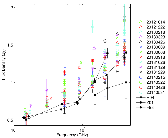
Figure 1: Spectrum of Sgr A* from VLA observations. Absolute flux densities are determined using long baseline data for epochs where it is available. We also plot results from historical measurements of the flux density: Falcke et al. (1998, F98), Zhao et al. (2001, Z01), and Herrnstein et al. (2004, H04). The F98 data consist of one measurement at a single epoch while Z01 and H04 represent averages over many years.

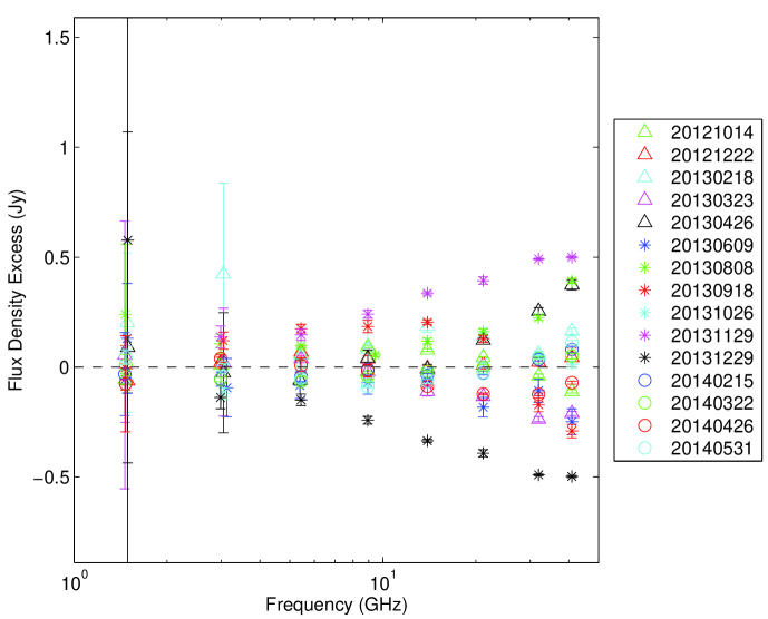
Figure 2: Differential spectrum of Sgr A* from all VLA epochs.

2.2 ALMA Observations

We carried out ALMA observations between mid-2013 and mid-2014 (Table 4), over eight epochs, each with band 6 (230 GHz) and band 7 (345 GHz) receivers. Details of the frequency setup are presented in Table 2. One spectral window in each band was configured with higher spectral resolution in order to permit detection of hydrogen recombination lines. We will discuss those results in a separate paper. Observations were snapshots with durations of a few minutes. The total flux density, corresponding to Stokes I, was produced by summing the response of parallel handed cross-correlations of the orthogonal linearly polarized feeds.

We set absolute amplitude calibration with observations of Titan and Neptune and set bandpass gains with observations of the compact source J1427-421. All calibrator sources and Sgr A* were phase-self-calibrated on timescales of a single integration (10 sec). For Sgr A*, phase self-calibration solutions were obtained only for baselines longer than $50\,k\lambda$. Flux densities for calibrators were determined by bootstrapping amplitude self-calibration solutions to the absolute flux density calibrator. Time-dependent amplitude gain solutions were applied to Sgr A*. Unfortunately, ALMA observations did not include system temperature measurements on Sgr A* itself. The pipeline software applied system temperatures obtained for J1733-130 (NRAO 530) to Sgr A*, which introduces an error because of the different atmospheric optical depth toward these two sources. To correct for this effect, we fitted system temperatures for all sources in each epoch to determine the atmospheric optical depth and then applied the correct system temperature to Sgr A*. Typical changes to the amplitude gain were a few percent, with a maximum value of 7%. Flux densities for Sgr A* were obtained through fitting a point-source of unknown flux to visibilities on baselines longer than $50\,k\lambda$. We report the results in Table 5. We do not report statistical errors on the flux densities because these are typically $\sim 1$ mJy, much less than the likely uncertainty from gain calibration errors for these bright sources. We show ALMA spectra for Sgr A* and all sources in Figure 3.

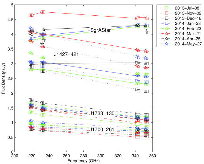
Figure 3: Spectrum of Sgr A* and calibrators from ALMA observations. Lines connect spectra for Sgr A* (solid), J1427-421 (dotted), J1733-130 (dashed), and J1700-261 (dash-dotted). Symbols and colors denote the observational epoch.

ALMA flux densities for the calibrators are consistent with recent SMA measurements of flux densities. We plot ALMA and SMA light curves for Sgr A* and J1733-130 in Figures 4 and 5. SMA data are described in the following Section. Where the data are contemporaneous, we see very good agreement in both ALMA bands.

The variability of the calibrators sets an upper bound on the calibration accuracy for Sgr A*. J1733-130, J1700-261, and J1427-421 show 5%, 9%, and 14% variability, respectively, in the fitted intensity at 230 GHz assuming a power-law spectrum for these sources. Thus, we take 5% as the systematic calibration error in the Sgr A* flux density.

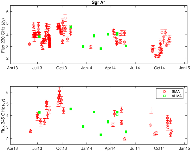
Figure 4: ALMA and SMA light curves at 230 GHz (top) and 345 GHz (bottom) for Sgr A*. Each ALMA spectral window is plotted, covering 218 to 235 GHz (top) and 341 to 355 GHz (bottom). The two lower frequency spectral windows for each ALMA band are plotted with filled symbols. These match most closely the plotted SMA flux densities, which are in the range 212 to 241 GHz and 331 to 356 GHz, respectively, and have mean frequencies of 221 and 338 GHz.

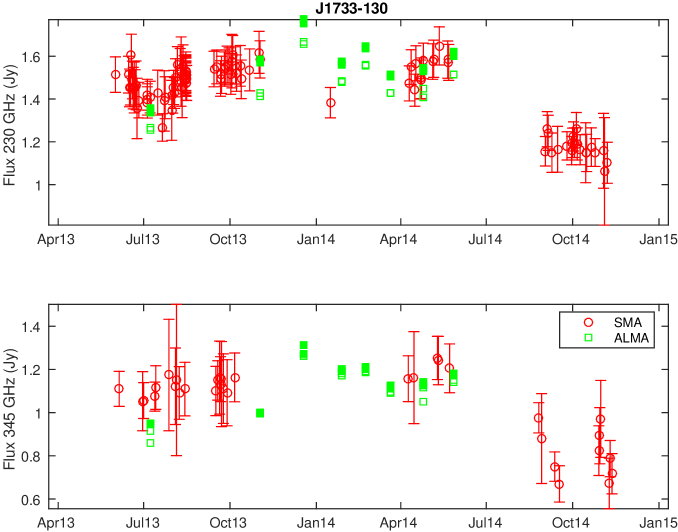
Figure 5: ALMA and SMA light curves at 230 GHz (top) and 345 GHz (bottom) for J1733-130. Symbols are the same as in Figure 4.

2.3 SMA Observations

Observations of the flux density of Sgr A* were obtained using the SMA, an interferometric array of eight 6-m diameter radio dishes located near the summit of Mauna Kea, Hawaii (Ho et al., 2004). In most cases the SMA was operating in a single receiver mode, providing 4 GHz continuum bandwidth in a single polarization, in two sidebands, with the array tuned to one of the three main SMA bands (1.3 mm, 1.1 mm and 870 micron).

Data were obtained during short ($\sim$20 min), self-contained observation sets, in which observations of Sgr A* alternated with those of the relatively nearby blazar J1733-130, and were bookended with observations of a flux standard (typically Neptune). These observations were “piggy backed” on full-track scheduled observations-of-the-day for the SMA. This explains the apparent randomness in sky frequencies. In addition, the flux densities were estimated from a measurements with a single linear polarization. The fractional linear polarization in Sgr A* is typically in the range of 5-10 percent and changes rapidly. The single polarization estimate of the flux density for a polarization of 10 percent has an rms error of 7 percent. This error is comparable to the level of the statistical errors. To this data set were added more extensive observations over several hours in dual polarization mode on 5 July and 15 Aug 2013, which allowed short-term monitoring.

Data from each observing period were calibrated with the millimeter interferometer reduction (MIR) suite of reduction routines developed by the SMA, involving removal of visibility phase scatter due to atmospheric instability and scaling visibility amplitude via comparison with the flux standard. Neptune was the primary flux standard used (85% of observations), with Uranus (13%) and Titan (2%) as the other standards. For Uranus and Neptune, we used the broadband spectral model from Griffin & Orton (1993). However, due to the presence of broad CO absorption in the spectrum of Neptune which is not included in the Griffin and Orton spectral fit, we opted to use data that were at least 8 GHz separated from either the CO(1-2) or CO(3-2) rotational transitions. For Titan, we used the spectral model developed by author Gurwell, which is now included in the CASA data reduction package as well (see Butler, 2012). In all cases the expected error on the flux density scale based upon using these models is  5%. On the other hand, since we are most interested in tracking changes in flux with time, the intrinsic bias in the flux density model is less important.

The presence of gas along the line of sight toward Sgr A* leads to deep absorption of the Sgr A* continuum at the CO transitions, as well as their isotopologues. For this reason, we masked spectral regions around these transitions in the Sgr A* data. Likewise, the structure of the visibility data from Sgr A* indicated we were sensitive to broad scale continuum emission from dust in the vicinity of Sgr A*. In order to limit our data to emission from Sgr A* itself, we used only visibility data from baselines that exceeded 35 k$\lambda$, or roughly scales of 6″or finer, which was sufficient to isolate Sgr A* from the broader diffuse emission.

Flux densities from the SMA for Sgr A* and J1733-130 are tabulated in Table 6.

3 Results

The mean spectrum of Sgr A* from VLA, ALMA, and SMA observations is presented in Table 7 and Figure 6, along with variability, minimum flux, and maximum flux. Variability is substantially stronger at millimeter wavelengths than at radio wavelengths. The ratio of the rms variability to the total flux density, known as the modulation index, is 8% at 40 GHz and below, while it is $\sim 20\%$ at millimeter wavelengths. This variability cannot be attributed to differences in calibration accuracy.

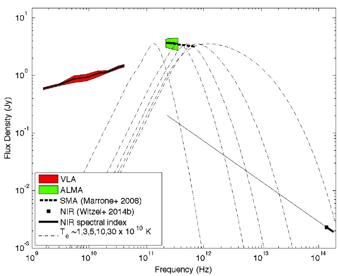
Figure 6: Mean spectrum of Sgr A* from VLA and ALMA observations. The solid black line shows the mean and the shaded regions show the $1\sigma$ boundaries for the flux density based on the rms of the variations. We also plot a curve showing the 230 to 690 GHz spectrum as measured by Marrone et al. (2006). We plot several model curves representing synchrotron emission from relativistic thermal Maxwell-Juttner distributions. We also plot NIR mean flux densities and spectral indices from Witzel et al. (2014b), along with a curve showing the extension of the NIR spectral index to shorter wavelengths (thin solid line). See text for details.

At VLA frequencies between 1 and 40 GHz, the mean spectral index $\alpha$ is $0.28\pm 0.03$ ($S\propto\nu^{\alpha}$) and shows evidence for steepening at short wavelengths. A mean spectral index of 0.5 between 40 and 218 GHz is required to connect the VLA and ALMA spectra, comparable to what has been seen previously (Falcke et al., 1998). We also fit the ALMA data with a power-law spectrum (Figure 7). The mean spectral index for frequencies between 217 and 355 GHz is $\alpha=-0.06\pm 0.26$, which is flatter and more variable than those of the calibrators. The calibrators have mean spectral indices between 217 and 355 GHz of $-0.67\pm 0.06$, $-0.56\pm 0.08$, and $-0.57\pm 0.07$ for J1733-130, J1700-261, and J1427-421, respectively.

Marrone et al. (2006) found that the 230 to 690 GHz spectral index ranged in four epochs from -0.4 to +0.2, with a mean of -0.13. Our results span the same range of $\alpha$ and are statistically indistinguishably from those of Marrone et al. (2006); that is, the spectrum is consistent with a flat or slightly declining power-law spectrum above 230 GHz. Assuming stationary statistics for Sgr A* between the early observations and these new observations, we conclude that there is no evidence for spectral curvature or greater steepening in the spectrum between 230 and 690 GHz.

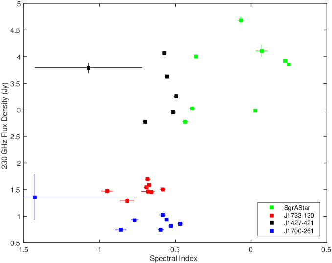
Figure 7: Fitted 230-GHz flux density and spectral index from the ALMA data (217 to 351 GHz) for Sgr A* and the calibrators.

The millimeter and submillimeter spectrum of Sgr A* indicates that the optical depth is $\sim 1$ at frequencies as high as 690 GHz. The result suggests that the source must be composed of stratified regions near the optically thick-to-thin transition in order to produce a near-flat synchrotron spectrum over this broad frequency range. A single optically thin synchrotron component cannot reproduce the spectrum. This spectrum can be explained in the context of the classical Blandford & Königl (1979) jet model, but also by inflowing accretion flow models with radially evolving density and magnetic fields together with some non-thermal particles (Yuan et al., 2003a).

Despite this degeneracy in the emission geometry, it is clear that above 350 GHz, Sgr A* has to become optically thin. This conclusion is supported by the transition to higher linear polarization at higher frequencies (Bower et al., 2003; Marrone et al., 2006), and the increased variability and power-law spectrum seen in the infrared band (e.g., Genzel et al., 2003; Ghez et al., 2004; Eckart et al., 2006; Witzel et al., 2012, 2014b).

Our simultaneous radio through submillimeter data can provide some interesting constraints on the underlying particle distribution, when put into context with the infrared measurements. In Fig. 6 we include the average IR flux based on VLT and Keck measurements (Witzel et al., 2012, 2014b). These results are consistent with a mean flux density of $\sim 3$ mJy in the $K_{s}$ band and a stable spectral index $\alpha\sim-0.6$ between $K_{s}$ and $H$ band. Previous estimates of the NIR spectral index appear to show steeper spectral indices but may have suffered from non-simultaneous observations of the variable flux density (e.g., Bremer et al., 2011). To illustrate the new limits on the radiating particle distributions, we plot for reference a series of synchrotron spectra from mildly relativistic thermal electrons in equipartition with the magnetic field, ranging from $1-30\times 10^{10}$ K, assuming an emission region of size $3r_{g}$. The observed brightness temperature of Sgr A* at 230 GHz is $\sim 6\times 10^{10}$ K (Doeleman et al., 2008). These are fiducial values spanning the range from the literature (see, e.g., Falcke & Markoff, 2013, and references therein), to illustrate how stratified, self-absorbed regions can add to a near-flat spectrum, but also to place some limits on the fraction and distribution of non-thermal particles present. The peak of a given temperature component can shift by a factor of a few in frequency for different emission size regions or energy partition between radiating particles and the magnetic energy density. However, it is clear that a peak temperature (in the plasma closest to the black hole) below a few $10^{10}$ K cannot account for the extension of the self-absorbed spectrum through the ALMA range shown, and that a peak temperature much higher than a few $10^{11}$ K would violate the IR limits. It is also clear from these spectra that a purely thermal distribution cannot account for the IR flux.

The intersection of the IR power-law with the intermediate ranges indicates that a non-thermal “tail” of particles is present, with normalization on the order of $\leq 1$% of the thermal peak. This fraction is consistent with the results of fits to Sgr A* in quiescence, using a self-consistent calculation of the particle distribution given a mechanism for injecting a power-law of nonthermal particles (Dibi et al., 2014) . Recent work exploring second-order acceleration processes in turbulent, magnetized plasmas by Lynn et al. (2014) shows the self-consistent production of a such a nonthermal tail; however, its slope and relation to the thermal peak may be difficult to match to these newest constraints. Therefore the combination of simultaneous ALMA (eventually using even higher frequency bands) and IR data offers the best constraints yet on the shape of the radiating particle distributions and nonthermal fraction. The results presented here can already be used to guide implementation of the inclusion of particle acceleration in semi-analytical models (e.g. Markoff et al., 2001; Yuan et al., 2003b; Broderick & Loeb, 2009) and in the so-called “painting” of GRMHD simulations to produce images (e.g., Dexter et al., 2012; Mościbrodzka & Falcke, 2013; Mościbrodzka et al., 2014; Chan et al., 2014). Simultaneous observations between ALMA, IR, and X-ray, particularly during flaring, would provide strong constraints on the upper extreme of the nonthermal population and accelerating mechanisms.

3.1 Presence of a Bow Shock

Bow shock emission from the interaction of G2 with the accretion flow was anticipated to appear and peak months before the center of mass reached periastron (Narayan et al., 2012). The bow shock would excite nonthermal electrons that then produce synchrotron radiation in the magnetic field of the accretion flow. The synchrotron radiation is expected to peak at frequencies near 1 GHz and decline with an optically thin power-law index $\sim-0.7$. The predicted peak flux density of the radio light curve scales with a number of factors, including the relative velocity of the cloud, the accretion flow density profile, the efficiency of nonthermal electron energy production, and the timescale for electrons to cool. Perhaps the most important term is the cross-sectional area of the shock as it impacts the accretion flow. Sa̧dowski et al. (2013) use the geometrical size of G2 as observed at large radii, $\sim 3\times 10^{30}{\rm\,cm^{2}}$. Shcherbakov (2014), on the other hand, constructs a magnetically arrested, tidally distorted cloud, which has an area $\sim 10^{29}{\rm\,cm^{2}}$. Crumley & Kumar (2013) model G2 as a wind driven from a hidden star with a radius that shrinks as the external pressure in the accretion flow increases, leading to a minimum area at periastron of $\sim 10^{28}{\rm\,cm^{2}}$. The flux density in all models scales linearly with the area. Thus, predictions of the 1 GHz excess flux density excess range from $>10$ Jy for some models to $<0.1$ Jy for others.

Synchrotron lifetimes for the radiating electrons in the accretion inflow are long, so the timescale for the radio emission is determined by the dynamics of the bow shock. Shcherbakov (2014) predicts a characteristic timescale of four months, which is comparable to predictions in other models.

The L band data alone in the first and last epochs of our experiment show that no significant secular change has occurred over the course of this experiment. Between October 2012 and May 2014, the 1.5 GHz flux density changed by at most 12 mJy (2%). We can examine in more detail whether there is evidence for shorter time scale variations through an analysis of all the measurements in the three lowest VLA frequency bands. We compute estimates of the flux density excess above the average at 1.0 GHz using low frequency measurements (Figure 8). We extrapolate the flux density excess at 1.5, 3.1, and 5.4 GHz to 1 GHz, assuming a power-law spectrum with index $\alpha=-0.7$, appropriate for optically thin synchrotron emission. At frequencies above 5 GHz, intrinsic variability rises rapidly and is likely to exceed estimates of any bow shock-related variability. 1.5 GHz results alone are sometimes only weakly sensitive to variations because of limited overlap in $(u,v)$ coverage for the most compact configurations.

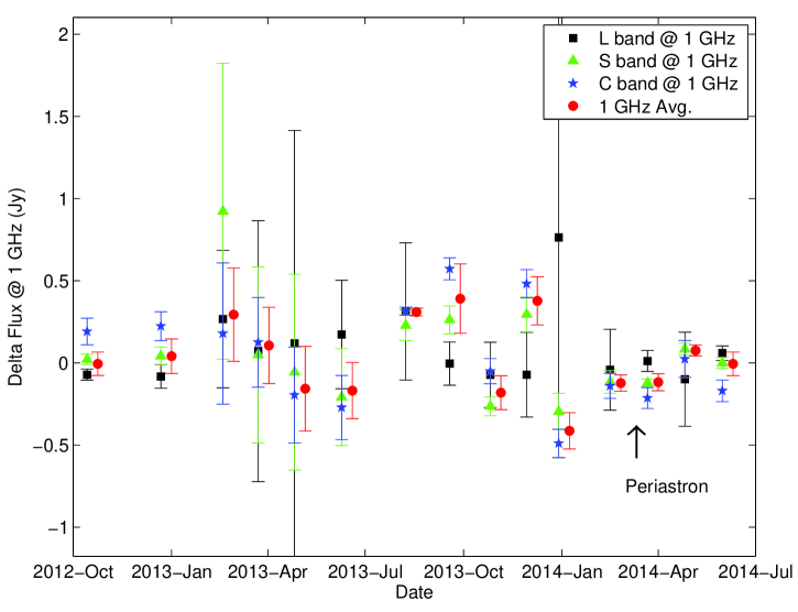
Figure 8: Estimates of the 1.0 GHz flux density excess above the average flux density. We extrapolate L, S, and C band (1.5, 3.1, 5.4 GHz) flux density excesses to 1 GHz using a power-law index of -0.7. The red symbols show the average of all three bands. Time is offset for the averages by 10 days for clarity in the figure. The arrow marks the estimated time of periastron (Pfuhl et al., 2015).

The average 1 GHz flux density excess computed in this way is only significantly non-zero for a single epoch, 2013 August 08, with a value of $0.310\pm 0.024$ Jy. The excess is positive and comparable for all three bands and very high significance at 5 GHz. The subsequent epoch, 2013 September 18, has a comparable value, $0.391\pm 0.211$ Jy, but much lower significance. The total flux density spectrum for 2013 August 08 is one of the most elevated across the band, with a peak flux density of 1.8 Jy at 40 GHz. These observations were obtained in a compact configuration and no total flux density measurements were obtained at 1.4 and 3.1 GHz.

For 11 of 15 epochs, the 95% confidence upper limit on 1 GHz flux density excess is 0.4 Jy. For the remaining four epochs, the upper limit is 0.8 Jy. A four-month moving average of the average 1 GHz flux has a peak at 0.3 Jy, centered on the 2013 August 08 epoch, and typical values of 0.1 Jy. These results clearly exclude an object with size $3\times 10^{30}{\rm\,cm^{2}}$. At 95% confidence, we can set an upper limit to the size of G2 of $\sim 2\times 10^{29}{\rm\,cm^{2}}$. This can be attributed to the magnetically arrested cloud derived by Shcherbakov (2014) or due to a pressure-confined stellar wind (Crumley & Kumar, 2013). Alternatively, the detailed model of the accretion flow structure could be in error.

3.2 Changes in the Mean Spectrum

The new data appear to show higher radio flux densities at frequencies $>2$ GHz over historical averages (Figure 1 and Table 7). The 40.9 GHz flux density, for instance, has a mean of 1.5 Jy and a range of 1.3 to 1.9 Jy, whereas Herrnstein et al. (2004) found a 43 GHz flux density mean of 1.0 Jy and a range of 0.6 to 1.9 Jy. Similar results with smaller amplitudes differences are apparent at lower frequencies. The flux densities from Falcke et al. (1998) and Zhao et al. (2001) are higher than those of Herrnstein et al. (2004) but still show a lower average flux density at most frequencies relative to the new VLA data. Zhao et al. (2001) presented many epochs of archival data obtained between 1979 and 1999. Herrnstein et al. (2004) reported over 100 epochs with regular monitoring from 2000 to 2003, while Falcke et al. (1998) is from a single-epoch simultaneous spectrum.

Over the whole radio spectrum, we infer an increase of $\sim 30\%$ relative to Herrnstein et al. (2004) and $\sim 10\%$ relative to Zhao et al. (2001) in the total flux density. These differences are comparable to the variability between Herrnstein et al. (2004) and Zhao et al. (2001) and consistent with variability seen in low-luminosity AGN (LLAGN) in general (Nagar et al., 2002; Ho, 2008). Thus, these differences cannot be attributed to any effects associated with the G2 periastron. The mean flux density that we measure at 21 GHz, $1.16\pm 0.05$ Jy, is comparable to the 22 GHz flux density measured over a similar time period with the Japanese VLBI Network, $1.23\pm 0.33$ Jy (Tsuboi et al., 2015). The lower variability in our result may reflect some of the difficulties of providing accurate amplitude calibration for VLBI arrays.

A comparison against historical millimeter and submillimeter flux densities also does not reveal any significant change. Dexter et al. (2014) presents historical data for Sgr A* at 230, 345, and 690 GHz with dates from 2001 through 2012. The flux densities from this paper span timescales from minutes to years and were obtained with multiple telescopes with varying calibration accuracy. The mean ALMA Band 6 (230 GHz) flux density is $3.6\pm 0.6$ Jy while the mean historical flux density at 230 GHz is $3.4\pm 0.5$ Jy. Similarly, for Band 7 (345 GHz) and historical 345 GHz data, we find $3.6\pm 0.8$ Jy and $3.0\pm 0.6$ Jy, respectively. Results from the SMA data are comparable. Thus, increases in the millimeter and submillimeter mean flux density are no more than 20% relative to historical averages, again consistent with typical LLAGN variability levels.

A Kolmogorov-Smirnov test shows that the ALMA and SMA measurements are consistent ($p\sim 0.1$) with originating from the same distribution. The ALMA and SMA measurements differ from the Dexter et al. (2014) measurements with varying significance. SMA 230 and 345 GHz data differ from the Dexter et al. (2014) distributions with $p<10^{-2}$, while the Band 6 (230 GHz) and Dexter 230 GHz and Band 7 and 345 GHz distributions differ with significances of $p=0.03$ and $p<10^{-3}$. These variations may be partly the result of different calibration accuracies and as the result of evolution of the light curves over $\sim 10$ yr. Similar to the case with the radio spectrum, there is no clear evidence that the millimeter and submillimeter changes are the result of the G2 periastron.

We have analyzed the light curve data for our measurements near 220 GHz from both ALMA and the SMA. There are 104 data points spanning an interval of 524 days with the shortest interval being 0.02 days. The data were binned in a sparsely filled array of 32,768 elements and Fourier transformed. The resulting spectrum was averaged into logarithmically spaced frequency intervals. The spectrum has a simple power law form characterized as $S\propto f^{\alpha}$ over a frequency interval of 0.04 to 2 cycle/day. $\alpha$ was found to be $-0.15\pm 0.08$. The error bar was determined by bootstrap resampling. This result is intuitively obvious from the light curve, i.e. the variations over a period of a few day are uncorrelated and have the same range as the variations over the entire data span. The spectral variations from historical data at millimeter/submillimeter wavelengths are known to approximate white noise at frequencies less than 3 cycles/day, with a steepening power law above that frequency (Dexter et al., 2014). It is plausible that an enhancement of emission caused by G2 might have produced long term variations indicative of red noise. However, there is no evidence for this effect.

4 Discussion and Conclusions

The spectrum of Sgr A* from radio to submillimeter wavelengths has remained remarkably stable over the past 30 years. Our new VLA, ALMA, and SMA results demonstrate that this stability has continued throughout the apparent periastron passage of G2. In the case of low-frequency emission, the absence of significant change permits us to constrain the size of the ensuing bow shock to be a factor of 30 smaller than the apparent G2 size observed with NIR wavelengths at larger distances from the black hole. These observations do not resolve the nature of G2. The smaller bow shock size is consistent with both cloud and stellar-wind models.

Witzel et al. (2014a) propose a model that may reconcile the apparently discrepant NIR continuum and spectroscopic observations and may also be consistent with our results. $L^{\prime}$ continuum observations reveal a compact source while Br-$\gamma$ observations reveal an extended source that appears to be tidally disrupted. Witzel et al. (2014a) argue that the continuum emission is the photosphere of a binary stellar merger, while the ionized emission represents a smaller tidally disrupted tail. The $L^{\prime}$ source has a cross-sectional area of $\sim 6\times 10^{27}$ cm², much less than our upper limit of $2\times 10^{29}$ cm². However, the size of the extended Br-$\gamma$ emission, which is consistent between VLT and Keck observations, primarily determines the creation of a bow shock. Some form of confinement for the diffuse gas appears to be important for attenuating the shock amplitude.

The lack of any enhanced short wavelength radio and millimeter emission from the black hole is also consistent with a compact size for G2. Simulations have shown that more extended objects are more readily disrupted and would therefore be more likely to have some gas initiate enhanced accretion onto the black hole.

At shorter wavelengths, the mean flux density has not increased by more than $\sim 20\%$ relative to historical averages. This is within the range of variations seen in the past and in other LLAGN. Thus, we cannot attribute any increase in the flux density to a G2-induced enhancement of the accretion rate. The amplitude and timescale for a change in the accretion rate, should G2 be fully disrupted, are uncertain. In order for the disrupted material to enhance the flux density, the gas must reach a radius of a few Schwarzschild radii to contribute to the accretion flow and/or enhance jet power. The free-fall time from $1000R_{Sch}$ is $t_{ff}\sim 0.1$ yr. If a fraction $f$ of the material were on a plunging orbit due to tidal disruption or a spread in orbital characteristics, we would have expected an enhancement of the overall flux density during these observations. The flux density should scale as

$${\Delta S\over S}=\left({fM_{G2}t_{ff}^{-1}\over\dot{M}}\right)^{\gamma},$$ (1)

where $\gamma\sim 1$ is a model-dependent constant for jet and accretion disk models (Falcke et al., 1993; Markoff et al., 2007; Mościbrodzka et al., 2012). For a G2 mass of $M_{G2}\approx 3M_{\earth}=10^{-5}M_{\odot}$ appropriate for the gas-cloud model and a steady-state accretion rate onto Sgr A* of $\dot{M}\sim 10^{-8}M_{\odot}\,{\rm yr^{-1}}$, and ${\Delta S\over S}\stackrel{{\scriptstyle\scriptstyle<}}{{\scriptstyle\sim}}0.2$, we find $f\stackrel{{\scriptstyle\scriptstyle<}}{{\scriptstyle\sim}}2\times 10^{-5}$ for $\gamma=1$. That is, very little of G2’s mass has yet accreted directly onto the black hole. Longer term monitoring (10 yr) will be sensitive to $f\stackrel{{\scriptstyle\scriptstyle>}}{{\scriptstyle\sim}}10^{-3}$ reaching the black hole through an increase of the average flux density. The bulk of the material is more likely to accrete on the viscous time scale, $t_{v}>>t_{ff}$. $t_{v}\sim t_{ff}\alpha_{v}^{-1}(H/R)^{-2}$, where $\alpha_{v}\sim 0.1$ – 1 is the viscous parameter and $H$ is the height at radius $R$. For reasonable parameters, $t_{v}\sim 0.1$ – 100 yr. Continued monitoring of the radio through millimeter flux densities can constrain further the properties and origin of G2 as well as the properties of the accretion flow at large radii.

The long-term stability of the radio/millimeter spectrum indicates that episodic events such as a fully disrupted cloud falling onto the black hole are rare. Such cloud disruptions may take place but they must have timescales that are long compared to the free-fall time.

We confirm a flat spectrum for Sgr A* emission in the millimeter/submillimeter regime. The emission is likely to originate from a stratified region with optical depth in transition between optically thick and thin. Optically thick emission at frequencies of $>230$ GHz may influence images obtained with the Event Horizon Telescope (Fish et al., 2013). Accretion disk models with tilted disks and/or high ratios of ion to electron temperature produce larger regions with optical depth greater than 1 (Mościbrodzka et al., 2009; Dexter & Fragile, 2013). Higher optical depths may obscure or complicate the interpretation of gravitational lensing effects such as the black hole shadow. On the other hand, higher optical depth in regions that are offset from the black hole as expected from Doppler boosting may enhance the contrast associated with geometric features. New ALMA measurements of the spectrum at frequencies from 100 to 950 GHz can resolve the uncertainty in the spectrum between the submillimeter and the NIR regime and assist in optimization of EHT observations.

Table 1: VLA Observations

Epoch	UT	Beam Q band	Beam L band	Configuration
		(arcsec2, deg)	(arcsec2, deg)
20121014	23:16 - 00:25	$0.13\times 0.11$ , 11.7	$2.97\times 2.45$, 45.1	A
20121222	17:30 - 18:39	$0.17\times 0.06$ , -15.8	$2.74\times 1.45$, -12.5	A
20130218	13:42 - 14:51	$4.36\times 1.65$ , -13.6	$79.21\times 74.20$, -72.9	D
20130323	12:02 - 13:11	$4.39\times 2.77$ , 29.3	$90.13\times 52.88$, 36.9	D
20130426	10:56 - 12:05	$4.43\times 2.83$ , 28.0	$88.42\times 46.85$, 50.2	D
20130609	06:25 - 07:34	$1.53\times 1.12$ , 42.9	$103.35\times 25.77$, -26.2	C
20130808	03:30 - 04:39	$1.39\times 0.93$ , 24.2	$38.22\times 19.51$, 29.1	C
20130918	01:33 - 02:42	$0.75\times 0.40$ , 63.1	$26.32\times 8.73$, 32.4	CnB
20131026	23:14 - 00:24	$0.43\times 0.27$ , 28.9	$12.05\times 5.85$, 23.4	B
20131129	19:46 - 20:55	$0.41\times 0.28$ , 23.4	$9.05\times 5.87$, 26.8	B
20131229	17:48 - 18:57	$0.43\times 0.30$ , 33.7	$38.08\times 14.34$, -1.3	B
20140215	14:11 - 15:21	$0.14\times 0.10$ , 37.3	$3.37\times 3.00$, -101.8	BnA
20140322	13:26 - 14:35	$0.13\times 0.09$ , 22.0	$3.26\times 1.53$, 24.0	A
20140426	10:19 - 11:28	$0.12\times 0.08$ , 27.0	$3.01\times 2.11$, -27.4	A
20140531	08:11 - 09:20	$0.28\times 0.15$ , 43.6	$3.41\times 2.07$, -28.1	A

Table 2: Frequency Coverage

Tel.	Band	$\nu_{lower}$	$\nu_{upper}$	$N_{ch}$
		(GHz)	(GHz)
VLA	L	994.0	2006.0	1024
VLA	S	1988.0	3948.0	1024
VLA	C	4488.0	6448.0	1024
VLA	X	7988.0	9948.0	1024
VLA	U	12988.0	14948.0	1024
VLA	K	20188.0	22148.0	1024
VLA	A	32008.0	31968.0	1024
VLA	Q	39988.0	41948.0	1024
ALMA	B6-1	217.0	219.0	128
ALMA	B6-2	219.0	221.0	128
ALMA	B6-3	231.0	232.9	3840
ALMA	B6-4	232.8	234.8	128
ALMA	B7-1	340.6	342.6	128
ALMA	B7-2	342.6	344.6	128
ALMA	B7-3	350.7	352.7	128
ALMA	B7-4	352.7	354.6	3840

Table 3: VLA Results

Epoch	Frequency	Flux Density	Delta Flux Density
	(GHz)	(Jy)	(Jy)
20121014	1.5	$0.578\pm 0.016$	$-0.055\pm 0.026$
20121014	3.0	$0.739\pm 0.045$	$0.010\pm 0.014$
20121014	5.4	$0.867\pm 0.031$	$0.059\pm 0.025$
20121014	8.9	$0.982\pm 0.031$	$0.093\pm 0.005$
20121014	13.9	$1.092\pm 0.006$	$0.078\pm 0.007$
20121014	21.1	$1.213\pm 0.007$	$0.045\pm 0.002$
20121014	32.0	$1.370\pm 0.011$	$-0.041\pm 0.009$
20121014	40.9	$1.427\pm 0.004$	$-0.110\pm 0.008$
20121222	1.5	$0.558\pm 0.029$	$-0.062\pm 0.054$
20121222	3.0	$0.691\pm 0.008$	$0.020\pm 0.025$
20121222	5.4	$0.876\pm 0.029$	$0.068\pm 0.027$
20121222	8.9	$0.952\pm 0.037$	$0.037\pm 0.015$
20121222	13.9	$1.009\pm 0.007$	$-0.004\pm 0.011$
20121222	21.1	$1.170\pm 0.012$	$0.010\pm 0.015$
20121222	32.0	$1.525\pm 0.102$	$0.022\pm 0.020$
20121222	40.9	$1.478\pm 0.052$	$0.043\pm 0.043$
20130218	1.5	…	$0.202\pm 0.317$
20130218	3.0	…	$0.424\pm 0.413$
20130218	5.4	…	$0.055\pm 0.131$
20130218	8.9	…	$0.081\pm 0.075$
20130218	13.9	$1.749\pm 0.088$	$0.186\pm 0.028$
20130218	21.1	$1.421\pm 0.021$	$0.140\pm 0.011$
20130218	32.0	$1.505\pm 0.015$	$0.059\pm 0.008$
20130218	40.9	$1.666\pm 0.040$	$0.163\pm 0.015$
20130323	1.5	…	$0.055\pm 0.610$
20130323	3.0	…	$0.023\pm 0.246$
20130323	5.4	…	$0.038\pm 0.083$
20130323	8.9	…	$-0.020\pm 0.026$
20130323	13.9	$1.455\pm 0.013$	$-0.111\pm 0.021$
20130323	21.1	$1.344\pm 0.035$	$-0.134\pm 0.015$
20130323	32.0	$1.274\pm 0.017$	$-0.237\pm 0.012$
20130323	40.9	$1.395\pm 0.018$	$-0.211\pm 0.009$
20130426	1.5	…	$0.090\pm 0.980$
20130426	3.0	…	$-0.026\pm 0.273$
20130426	5.4	…	$-0.060\pm 0.090$
20130426	8.9	…	$0.041\pm 0.037$
20130426	13.9	…	$-0.009\pm 0.021$
20130426	21.1	$1.562\pm 0.029$	$0.122\pm 0.009$
20130426	32.0	$1.648\pm 0.017$	$0.254\pm 0.015$
20130426	40.9	$1.882\pm 0.132$	$0.374\pm 0.023$
20130609	1.5	…	$0.131\pm 0.250$
20130609	3.1	…	$-0.094\pm 0.133$
20130609	5.4	$1.097\pm 0.105$	$-0.083\pm 0.060$
20130609	8.9	$1.059\pm 0.069$	$-0.070\pm 0.053$
20130609	13.9	$1.137\pm 0.040$	$-0.060\pm 0.006$
20130609	21.1	$1.037\pm 0.219$	$-0.183\pm 0.045$
20130609	32.0	$1.286\pm 0.051$	$-0.108\pm 0.052$
20130609	40.9	$1.278\pm 0.058$	$-0.249\pm 0.059$
20130808	1.5	…	$0.240\pm 0.319$
20130808	3.0	…	$0.106\pm 0.043$
20130808	5.4	$0.835\pm 0.086$	$0.096\pm 0.007$
20130808	9.4	$1.276\pm 0.022$	$0.055\pm 0.008$
20130808	13.9	$1.273\pm 0.038$	$0.118\pm 0.013$
20130808	21.1	$1.335\pm 0.031$	$0.161\pm 0.013$
20130808	32.0	$1.596\pm 0.006$	$0.225\pm 0.010$
20130808	40.9	$1.826\pm 0.014$	$0.391\pm 0.011$
20130918	1.5	…	$-0.003\pm 0.100$
20130918	3.0	$0.796\pm 0.025$	$0.120\pm 0.039$
20130918	5.4	$1.134\pm 0.032$	$0.175\pm 0.020$
20130918	8.9	$1.190\pm 0.023$	$0.185\pm 0.028$
20130918	13.9	$1.295\pm 0.014$	$0.204\pm 0.011$
20130918	21.1	$1.336\pm 0.013$	$0.129\pm 0.016$
20130918	32.0	$1.227\pm 0.031$	$-0.172\pm 0.031$
20130918	40.9	$1.275\pm 0.031$	$-0.291\pm 0.031$
20131026	1.5	$0.588\pm 0.037$	$-0.055\pm 0.150$
20131026	3.0	$0.659\pm 0.052$	$-0.121\pm 0.026$
20131026	5.4	$0.826\pm 0.020$	$-0.015\pm 0.023$
20131026	8.9	$0.945\pm 0.030$	$-0.066\pm 0.025$
20131026	13.9	$1.085\pm 0.015$	$-0.016\pm 0.008$
20131026	21.1	$1.215\pm 0.011$	$0.022\pm 0.003$
20131026	32.0	$1.392\pm 0.004$	$0.057\pm 0.007$
20131026	40.9	$1.472\pm 0.006$	$0.013\pm 0.014$
20131129	1.5	$0.683\pm 0.025$	$-0.055\pm 0.197$
20131129	3.0	$0.896\pm 0.150$	$0.137\pm 0.049$
20131129	5.4	$0.782\pm 0.044$	$0.147\pm 0.026$
20131129	8.9	$1.012\pm 0.028$	$0.241\pm 0.018$
20131129	13.9	$1.177\pm 0.022$	$0.335\pm 0.008$
20131129	21.1	$1.388\pm 0.028$	$0.393\pm 0.017$
20131129	32.0	$1.636\pm 0.009$	$0.492\pm 0.003$
20131129	40.9	$1.829\pm 0.032$	$0.499\pm 0.005$
20131229	1.5	…	$0.577\pm 1.013$
20131229	3.0	$0.729\pm 0.043$	$-0.138\pm 0.052$
20131229	5.4	$0.647\pm 0.062$	$-0.149\pm 0.026$
20131229	8.9	$0.791\pm 0.025$	$-0.242\pm 0.018$
20131229	13.9	$0.887\pm 0.028$	$-0.335\pm 0.008$
20131229	21.1	$0.999\pm 0.013$	$-0.392\pm 0.016$
20131229	32.0	$1.146\pm 0.005$	$-0.490\pm 0.004$
20131229	40.9	$1.334\pm 0.054$	$-0.498\pm 0.005$
20140215	1.5	$0.538\pm 0.095$	$-0.032\pm 0.189$
20140215	3.0	$0.680\pm 0.033$	$-0.054\pm 0.032$
20140215	5.4	$0.720\pm 0.040$	$-0.043\pm 0.023$
20140215	8.9	$0.877\pm 0.022$	$-0.010\pm 0.020$
20140215	13.9	$0.970\pm 0.012$	$-0.038\pm 0.009$
20140215	21.1	$1.135\pm 0.008$	$-0.027\pm 0.009$
20140215	32.0	$1.374\pm 0.003$	$0.035\pm 0.007$
20140215	40.9	$1.556\pm 0.015$	$0.080\pm 0.014$
20140322	1.5	$0.597\pm 0.056$	$0.009\pm 0.049$
20140322	3.0	$0.682\pm 0.025$	$-0.056\pm 0.011$
20140322	5.4	$0.999\pm 0.042$	$-0.065\pm 0.019$
20140322	8.9	$0.860\pm 0.017$	$-0.042\pm 0.013$
20140322	13.9	$1.001\pm 0.015$	$-0.020\pm 0.005$
20140322	21.1	$1.166\pm 0.008$	$-0.003\pm 0.013$
20140322	32.0	$1.392\pm 0.002$	$0.042\pm 0.004$
20140322	40.9	$1.526\pm 0.004$	$0.050\pm 0.013$
20140426	1.5	$0.512\pm 0.077$	$-0.076\pm 0.219$
20140426	3.0	$0.775\pm 0.039$	$0.039\pm 0.017$
20140426	5.4	$0.776\pm 0.068$	$0.007\pm 0.034$
20140426	8.9	$0.862\pm 0.011$	$-0.016\pm 0.029$
20140426	13.9	$0.944\pm 0.009$	$-0.088\pm 0.005$
20140426	21.1	$1.057\pm 0.005$	$-0.122\pm 0.004$
20140426	32.0	$1.264\pm 0.006$	$-0.124\pm 0.006$
20140426	40.9	$1.466\pm 0.005$	$-0.071\pm 0.007$
20140531	1.5	$0.590\pm 0.009$	$0.045\pm 0.034$
20140531	3.0	$0.734\pm 0.035$	$-0.000\pm 0.015$
20140531	5.4	$0.828\pm 0.043$	$-0.052\pm 0.020$
20140531	8.9	$0.891\pm 0.015$	$-0.089\pm 0.005$
20140531	13.9	$1.019\pm 0.011$	$-0.065\pm 0.008$
20140531	21.1	$1.166\pm 0.002$	$-0.030\pm 0.001$
20140531	32.0	$1.428\pm 0.058$	$0.044\pm 0.008$
20140531	40.9	$1.871\pm 0.177$	$0.112\pm 0.008$

Table 4: ALMA Observations

Epoch	UT	Beam B6 (230 GHz)	Beam B7 (345 GHz)	Flux Cal.
		(arcsec2, deg)	(arcsec2, deg)
20130708	02:14-02:44	$1.14\times 0.53$, 65.1	$0.38\times 0.29$, 73.8	Titan
20131102	22:39-22:57	$0.91\times 0.46$, -84.2	$0.51\times 0.30$, -87.2	Neptune
20131218	14:07-14:27	$1.36\times 0.64$, 88.3	$0.93\times 0.44$, 86.0	Titan
20140128	10:26-10:44	$2.39\times 0.78$, 78.8	$1.64\times 0.52$, 77.6	Titan
20140222	09:20-09:45	$1.89\times 0.92$, 69.3	$1.28\times 0.62$, 68.2	Titan
20140321	09:17-09:35	$0.99\times 0.67$, 79.3	$0.65\times 0.43$, 77.1	Titan
20140425	06:59-07:29	$0.71\times 0.58$, 78.7	$0.45\times 0.38$, 88.8	Titan
20140527	05:47-06:06	$0.62\times 0.50$, -75.2	$0.40\times 0.33$, -75.8	Titan

Table 5: ALMA Results

Epoch	Source	Flux Density (Jy)
		218.0 GHz	220.0 GHz	231.9 GHz	233.8 GHz	341.6 GHz	343.6 GHz	351.7 GHz	353.6 GHz
20130708	SgrAStar	3.792	3.795	3.872	3.892	4.259	4.278	4.270	4.265
20131102	SgrAStar	4.635	4.649	4.752	4.758	4.537	4.564	4.569	4.537
20131218	SgrAStar	2.976	2.970	2.997	3.010	3.032	3.046	3.012	3.003
20140128	SgrAStar	3.868	3.868	3.944	3.957	4.293	4.313	4.309	4.294
20140222	SgrAStar	2.811	2.803	2.800	2.801	2.332	2.341	2.311	2.301
20140321	SgrAStar	4.078	4.047	3.983	4.002	3.476	3.447	3.428	3.406
20140425	SgrAStar	4.121	4.111	4.004	4.163	4.296	4.287	4.295	4.064
20140527	SgrAStar	3.054	3.048	3.054	3.051	2.587	2.596	2.568	2.556
20130708	J1733-130	1.359	1.337	1.256	1.264	0.952	0.951	0.917	0.857
20131102	J1733-130	1.586	1.570	1.429	1.413	0.998	0.994	0.995	0.998
20131218	J1733-130	1.771	1.754	1.668	1.657	1.311	1.273	1.261	1.263
20140128	J1733-130	1.576	1.561	1.477	1.482	1.203	1.190	1.181	1.173
20140222	J1733-130	1.649	1.638	1.557	1.560	1.214	1.201	1.192	1.187
20140321	J1733-130	1.517	1.502	1.426	1.426	1.125	1.109	1.097	1.092
20140425	J1733-130	1.545	1.532	1.406	1.449	1.140	1.126	1.114	1.053
20140527	J1733-130	1.619	1.600	1.517	1.514	1.179	1.169	1.142	1.150
20131218	J1427-421	2.899	2.876	2.739	2.750	2.131	2.079	2.065	2.058
20140128	J1427-421	3.073	3.041	2.908	2.907	2.422	2.387	2.375	2.379
20140222	J1427-421	3.370	3.353	3.201	3.206	2.665	2.658	2.639	2.645
20140321	J1427-421	3.773	3.735	3.570	3.582	2.931	2.900	2.859	2.856
20140425	J1427-421	4.015	3.984	3.669	3.799	-0.019	-0.019	-0.016	-0.015
20140527	J1427-421	4.227	4.187	4.002	4.002	3.253	3.217	3.191	3.176
20130708	J1700-261	0.967	0.962	0.914	0.916	0.701	0.685	0.666	0.651
20131102	J1700-261	0.791	0.784	0.721	0.720	0.517	0.518	0.525	0.522
20131218	J1700-261	0.774	0.775	0.732	0.734	0.592	0.583	0.574	0.585
20140128	J1700-261	0.887	0.882	0.842	0.846	0.716	0.707	0.706	0.700
20140222	J1700-261	0.969	0.961	0.921	0.924	0.749	0.744	0.738	0.738
20140321	J1700-261	0.846	0.838	0.800	0.804	0.664	0.657	0.650	0.646
20140425	J1700-261	…	…	…	…	0.773	0.763	0.757	0.723
20140527	J1700-261	1.072	1.062	1.004	1.005	0.824	0.799	0.803	0.799

Table 6: SMA Results

Epoch	UT	Frequency	$S_{\rm Sgr~{}A*}$	$S_{\rm J1733-130}$
		(GHz)	(Jy)	(Jy)
20130601	13:18	218.60	$3.217\pm 0.168$	$1.514\pm 0.083$
20130605	13:23	336.40	$2.680\pm 0.145$	$1.110\pm 0.081$
20130609	13:21	271.80	$4.743\pm 0.246$	$1.276\pm 0.081$
20130610	13:32	265.99	$3.237\pm 0.188$	$1.271\pm 0.106$
20130612	12:15	271.79	$4.055\pm 0.206$	$1.319\pm 0.078$
20130615	12:08	218.48	$3.951\pm 0.210$	$1.514\pm 0.086$
20130616	12:53	218.95	$3.956\pm 0.210$	$1.452\pm 0.088$
20130617	12:15	219.71	$4.836\pm 0.245$	$1.452\pm 0.080$
20130618	12:03	218.47	$4.605\pm 0.237$	$1.605\pm 0.098$
20130619	12:41	218.95	$3.618\pm 0.193$	$1.489\pm 0.088$
20130620	12:13	214.60	$3.982\pm 0.207$	$1.451\pm 0.097$
20130621	12:37	218.77	$4.018\pm 0.213$	$1.454\pm 0.119$
20130622	12:41	218.93	$3.957\pm 0.205$	$1.451\pm 0.086$
20130623	11:39	218.68	$4.079\pm 0.249$	$1.464\pm 0.114$
20130624	12:10	218.75	$3.986\pm 0.224$	$1.356\pm 0.141$
20130626	11:43	218.68	$3.980\pm 0.211$	$1.395\pm 0.083$
20130630	12:13	333.40	$3.832\pm 0.259$	$1.053\pm 0.137$
20130701	10:35	342.96	$4.023\pm 0.212$	$1.056\pm 0.083$
20130705	07:18	226.86	$4.204\pm 0.228$	$1.384\pm 0.073$
20130705	08:55	226.86	$4.796\pm 0.245$	$1.420\pm 0.072$
20130705	11:41	226.86	$3.980\pm 0.204$	$1.398\pm 0.073$
20130708	11:07	218.87	$3.989\pm 0.205$	$1.409\pm 0.074$
20130713	10:55	336.38	$3.524\pm 0.195$	$1.074\pm 0.067$
20130714	10:44	333.40	$3.267\pm 0.194$	$1.116\pm 0.101$
20130716	10:36	218.84	$3.265\pm 0.184$	$1.430\pm 0.105$
20130717	11:05	265.99	$3.439\pm 0.181$	$1.263\pm 0.088$
20130719	10:32	265.97	$3.315\pm 0.170$	$1.090\pm 0.064$
20130720	10:42	271.78	$3.597\pm 0.188$	$1.206\pm 0.080$
20130721	10:30	218.69	$2.887\pm 0.152$	$1.267\pm 0.064$
20130723	10:43	218.84	$3.463\pm 0.215$	$1.391\pm 0.141$
20130724	10:45	218.90	$3.522\pm 0.207$	$1.406\pm 0.098$
20130728	10:12	336.07	$3.467\pm 0.268$	$1.174\pm 0.258$
20130731	10:07	218.79	$3.869\pm 0.401$	$1.347\pm 0.140$
20130801	09:58	218.79	$3.475\pm 0.248$	$1.419\pm 0.085$
20130802	09:38	218.79	$4.200\pm 0.217$	$1.454\pm 0.080$
20130803	09:01	218.82	$4.740\pm 0.244$	$1.428\pm 0.072$
20130804	08:46	334.73	$5.044\pm 0.287$	$1.122\pm 0.177$
20130804	09:39	215.44	$4.727\pm 0.250$	$1.499\pm 0.089$
20130805	08:51	336.98	$4.854\pm 0.340$	$1.151\pm 0.350$
20130806	09:49	218.96	$3.788\pm 0.205$	$1.558\pm 0.087$
20130808	09:09	333.98	$4.014\pm 0.291$	$1.091\pm 0.122$
20130809	08:34	218.85	$4.298\pm 0.224$	$1.538\pm 0.098$
20130810	09:13	218.77	$4.356\pm 0.333$	$1.528\pm 0.162$
20130811	08:55	218.77	$3.857\pm 0.294$	$1.451\pm 0.138$
20130812	09:10	218.99	$3.744\pm 0.205$	$1.557\pm 0.096$
20130813	09:10	218.66	$4.642\pm 0.246$	$1.513\pm 0.089$
20130814	08:19	334.00	$4.469\pm 0.275$	$1.109\pm 0.124$
20130815	03:27	226.85	$3.307\pm 0.172$	$1.517\pm 0.085$
20130815	03:56	226.85	$3.228\pm 0.173$	$1.475\pm 0.081$
20130815	04:27	226.85	$3.114\pm 0.163$	$1.514\pm 0.084$
20130815	04:56	226.85	$3.062\pm 0.165$	$1.523\pm 0.084$
20130815	05:27	226.85	$3.118\pm 0.164$	$1.510\pm 0.083$
20130815	05:56	226.85	$3.641\pm 0.192$	$1.490\pm 0.078$
20130815	06:25	226.85	$3.623\pm 0.186$	$1.510\pm 0.081$
20130815	06:57	226.85	$3.582\pm 0.184$	$1.497\pm 0.080$
20130815	07:25	226.85	$3.638\pm 0.188$	$1.516\pm 0.088$
20130815	08:01	226.85	$3.742\pm 0.196$	$1.494\pm 0.078$
20130815	08:26	226.85	$3.533\pm 0.182$	$1.495\pm 0.083$
20130815	08:53	226.85	$3.529\pm 0.182$	$1.497\pm 0.081$
20130815	09:24	226.85	$3.332\pm 0.176$	$1.530\pm 0.090$
20130816	08:12	220.59	$3.149\pm 0.165$	$1.475\pm 0.082$
20130914	06:24	218.93	$4.685\pm 0.246$	$1.540\pm 0.083$
20130916	06:28	331.32	$5.048\pm 0.282$	$1.100\pm 0.114$
20130917	06:43	219.19	$4.736\pm 0.238$	$1.550\pm 0.079$
20130918	06:15	331.31	$5.492\pm 0.280$	$1.149\pm 0.091$
20130920	06:12	331.31	$5.310\pm 0.318$	$1.162\pm 0.169$
20130921	05:01	219.87	$4.778\pm 0.242$	$1.496\pm 0.083$
20130921	05:01	334.79	$5.751\pm 0.297$	$1.155\pm 0.104$
20130922	05:49	220.64	$4.566\pm 0.233$	$1.513\pm 0.087$
20130922	05:49	355.92	$6.090\pm 0.342$	$1.132\pm 0.197$
20130924	05:38	331.37	$5.093\pm 0.297$	$1.111\pm 0.161$
20130925	06:30	219.21	$4.271\pm 0.216$	$1.540\pm 0.080$
20130926	06:28	218.93	$4.345\pm 0.219$	$1.548\pm 0.081$
20130928	05:24	220.71	$4.229\pm 0.214$	$1.561\pm 0.086$
20130928	05:24	355.92	$5.330\pm 0.294$	$1.092\pm 0.153$
20130930	05:54	220.28	$4.335\pm 0.219$	$1.557\pm 0.082$
20131002	05:32	220.27	$5.007\pm 0.261$	$1.517\pm 0.095$
20131003	05:30	220.27	$3.438\pm 0.190$	$1.577\pm 0.125$
20131004	04:22	219.85	$5.101\pm 0.260$	$1.607\pm 0.090$
20131006	05:06	334.92	$4.424\pm 0.244$	$1.163\pm 0.113$
20131007	05:00	220.27	$4.574\pm 0.232$	$1.557\pm 0.087$
20131008	04:37	239.61	$4.035\pm 0.215$	$1.521\pm 0.085$
20131012	04:26	218.83	$5.420\pm 0.290$	$1.555\pm 0.095$
20131013	04:27	218.83	$4.530\pm 0.235$	$1.492\pm 0.090$
20131022	04:08	239.61	$3.630\pm 0.190$	$1.536\pm 0.098$
20131101	03:25	218.90	$4.532\pm 0.235$	$1.618\pm 0.098$
20131102	03:16	219.37	$4.118\pm 0.219$	$1.585\pm 0.087$
20140116	19:58	225.02	$2.957\pm 0.150$	$1.383\pm 0.071$
20140408	13:59	266.10	$3.482\pm 0.180$	$1.271\pm 0.070$
20140409	16:42	334.01	$3.232\pm 0.183$	$1.157\pm 0.106$
20140410	17:01	219.74	$4.211\pm 0.214$	$1.473\pm 0.082$
20140412	16:41	218.92	$4.361\pm 0.221$	$1.549\pm 0.081$
20140415	16:22	356.05	$4.146\pm 0.280$	$1.162\pm 0.213$
20140416	16:40	218.78	$3.820\pm 0.192$	$1.441\pm 0.075$
20140417	16:37	218.43	$3.976\pm 0.203$	$1.567\pm 0.082$
20140422	16:10	220.56	$3.228\pm 0.202$	$1.491\pm 0.091$
20140423	16:47	218.97	$3.479\pm 0.188$	$1.497\pm 0.095$
20140425	15:19	215.27	$3.301\pm 0.179$	$1.578\pm 0.083$
20140505	15:01	219.02	$4.022\pm 0.212$	$1.575\pm 0.083$
20140506	14:49	218.74	$3.409\pm 0.176$	$1.588\pm 0.087$
20140510	13:43	336.95	$4.499\pm 0.237$	$1.253\pm 0.100$
20140511	14:15	336.95	$3.387\pm 0.182$	$1.241\pm 0.112$
20140512	15:43	218.93	$4.155\pm 0.214$	$1.648\pm 0.089$
20140521	14:31	219.00	$3.368\pm 0.181$	$1.584\pm 0.087$
20140522	14:12	219.00	$4.127\pm 0.215$	$1.571\pm 0.084$
20140523	14:15	332.14	$1.999\pm 0.135$	$1.205\pm 0.113$
20140826	08:13	335.55	$3.173\pm 0.168$	$0.976\pm 0.070$
20140829	07:09	353.75	$4.458\pm 0.271$	$0.880\pm 0.208$
20140902	07:39	241.36	$2.955\pm 0.153$	$1.156\pm 0.069$
20140903	07:45	271.52	$2.799\pm 0.145$	$1.054\pm 0.069$
20140904	07:07	220.77	$2.586\pm 0.138$	$1.259\pm 0.082$
20140905	07:20	220.77	$2.924\pm 0.154$	$1.242\pm 0.082$
20140909	07:18	241.36	$3.020\pm 0.176$	$1.149\pm 0.092$
20140912	06:06	335.59	$2.421\pm 0.136$	$0.750\pm 0.068$
20140915	05:45	220.20	$2.158\pm 0.153$	$1.165\pm 0.107$
20140917	06:19	333.39	$2.500\pm 0.141$	$0.670\pm 0.084$
20140925	05:40	214.17	$2.154\pm 0.119$	$1.181\pm 0.066$
20140930	05:15	219.42	$2.309\pm 0.142$	$1.159\pm 0.066$
20141001	05:50	213.23	$2.747\pm 0.159$	$1.195\pm 0.069$
20141002	05:05	213.44	$3.456\pm 0.182$	$1.225\pm 0.068$
20141003	05:39	219.52	$3.191\pm 0.178$	$1.196\pm 0.069$
20141005	05:25	218.68	$2.557\pm 0.160$	$1.262\pm 0.075$
20141006	05:36	218.67	$2.659\pm 0.167$	$1.190\pm 0.075$
20141009	05:18	218.62	$4.222\pm 0.250$	$1.163\pm 0.070$
20141015	05:24	219.71	$3.514\pm 0.317$	$1.149\pm 0.140$
20141016	05:16	218.90	$3.804\pm 0.259$	$1.148\pm 0.087$
20141021	05:03	220.26	$4.190\pm 0.235$	$1.175\pm 0.090$
20141025	04:09	219.42	$3.139\pm 0.170$	$1.150\pm 0.065$
20141029	04:10	335.58	$3.783\pm 0.227$	$0.824\pm 0.115$
20141030	04:03	335.58	$3.365\pm 0.219$	$0.893\pm 0.130$
20141031	04:18	356.16	$2.961\pm 0.282$	$0.971\pm 0.178$
20141103	04:10	220.27	$3.502\pm 0.316$	$1.158\pm 0.175$
20141104	04:09	218.63	$3.701\pm 0.346$	$1.062\pm 0.251$
20141107	03:49	220.26	$3.680\pm 0.281$	$1.102\pm 0.096$
20141109	03:55	333.33	$3.531\pm 0.252$	$0.672\pm 0.117$
20141110	03:46	333.36	$2.359\pm 0.199$	$0.787\pm 0.084$
20141112	03:51	333.36	$2.609\pm 0.201$	$0.717\pm 0.093$

Table 7: Mean Spectrum of Sgr A* 

Freq.	Mean Flux Density	Standard Dev.	Minimum Flux Density	Maximum Flux Density	$N_{\rm epoch}$	Tel.
(GHz)	(Jy)	(Jy)	(Jy)	(Jy)
1.6	0.592	0.028	0.512	0.683	8	VLA
3.1	0.702	0.032	0.659	0.896	10	VLA
5.4	0.870	0.118	0.647	1.134	12	VLA
9.0	0.932	0.129	0.791	1.276	12	VLA
14.0	1.075	0.135	0.887	1.749	14	VLA
21.1	1.164	0.052	0.999	1.562	15	VLA
32.0	1.382	0.087	1.146	1.648	15	VLA
40.9	1.485	0.073	1.275	1.882	15	VLA
218.0	3.667	0.650	2.811	4.635	8	ALMA
220.0	3.661	0.652	2.803	4.649	8	ALMA
231.9	3.676	0.664	2.800	4.752	8	ALMA
233.8	3.704	0.680	2.801	4.758	8	ALMA
341.6	3.602	0.866	2.332	4.537	8	ALMA
343.6	3.609	0.870	2.341	4.564	8	ALMA
351.7	3.595	0.884	2.311	4.569	8	ALMA
353.6	3.553	0.860	2.301	4.537	8	ALMA
216.8	3.677	0.762	2.154	5.420	68	SMA
223.9	3.391	0.489	2.586	4.796	23	SMA
238.2	3.310	0.424	2.955	4.035	4	SMA
266.8	3.369	0.096	3.237	3.482	4	SMA
274.0	3.526	0.697	2.799	4.743	4	SMA
331.1	3.205	1.074	1.999	5.492	14	SMA
338.3	3.436	0.863	2.421	5.751	13	SMA
352.6	4.890	0.721	4.146	6.090	4	SMA

References

- Akiyama et al. (2014) Akiyama, K., Kino, M., Sohn, B., Lee, S., Trippe, S., & Honma, M. 2014, in IAU Symposium, Vol. 303, IAU Symposium, ed. L. O. Sjouwerman, C. C. Lang, & J. Ott, 288–292
- Anninos et al. (2012) Anninos, P., Fragile, P. C., Wilson, J., & Murray, S. D. 2012, ApJ, 759, 132
- Blandford & Königl (1979) Blandford, R. D. & Königl, A. 1979, 232, 34
- Bower et al. (2003) Bower, G. C., Wright, M. C. H., Falcke, H., & Backer, D. C. 2003, 588, 331
- Bremer et al. (2011) Bremer, M., Witzel, G., Eckart, A., Zamaninasab, M., Buchholz, R. M., Schödel, R., Straubmeier, C., García-Marín, M., & Duschl, W. 2011, A&A, 532, A26
- Broderick & Loeb (2009) Broderick, A. E. & Loeb, A. 2009, ApJ, 697, 1164
- Butler (2012) Butler, B. 2012, ALMA Memo Series, 594
- Chan et al. (2014) Chan, C.-K., Psaltis, D., Ozel, F., Narayan, R., & Sadowski, A. 2014, ”subm. (arXiv:1410.3492)”
- Chandler & Sjouwerman (2013) Chandler, C. J. & Sjouwerman, L. O. 2013, The Astronomer’s Telegram, 5153, 1
- Crumley & Kumar (2013) Crumley, P. & Kumar, P. 2013, MNRAS, 436, 1955
- Degenaar et al. (2013) Degenaar, N., Reynolds, M. T., Miller, J. M., Kennea, J. A., & Wijnands, R. 2013, The Astronomer’s Telegram, 5006, 1
- Dexter & Fragile (2013) Dexter, J. & Fragile, P. C. 2013, MNRAS, 432, 2252
- Dexter et al. (2014) Dexter, J., Kelly, B., Bower, G. C., Marrone, D. P., Stone, J., & Plambeck, R. 2014, MNRAS, 442, 2797
- Dexter et al. (2012) Dexter, J., McKinney, J. C., & Agol, E. 2012, MNRAS, 421, 1517
- Dibi et al. (2014) Dibi, S., Markoff, S., Belmont, R., Malzac, J., Barrière, N. M., & Tomsick, J. A. 2014, MNRAS, 441, 1005
- Do et al. (2009) Do, T., Ghez, A. M., Morris, M. R., Yelda, S., Meyer, L., Lu, J. R., Hornstein, S. D., & Matthews, K. 2009, ApJ, 691, 1021
- Dodds-Eden et al. (2011) Dodds-Eden, K., Gillessen, S., Fritz, T. K., Eisenhauer, F., Trippe, S., Genzel, R., Ott, T., Bartko, H., Pfuhl, O., Bower, G., Goldwurm, A., Porquet, D., Trap, G., & Yusef-Zadeh, F. 2011, ApJ, 728, 37
- Doeleman et al. (2008) Doeleman, S. S., Weintroub, J., Rogers, A. E. E., Plambeck, R., Freund, R., Tilanus, R. P. J., Friberg, P., Ziurys, L. M., Moran, J. M., Corey, B., Young, K. H., Smythe, D. L., Titus, M., Marrone, D. P., Cappallo, R. J., Bock, D., Bower, G. C., Chamberlin, R., Davis, G. R., Krichbaum, T. P., Lamb, J., Maness, H., Niell, A. E., Roy, A., Strittmatter, P., Werthimer, D., Whitney, A. R., & Woody, D. 2008, Nature, 455, 78
- Eatough et al. (2013) Eatough, R. P., Falcke, H., Karuppusamy, R., Lee, K. J., Champion, D. J., Keane, E. F., Desvignes, G., Schnitzeler, D. H. F. M., Spitler, L. G., Kramer, M., Klein, B., Bassa, C., Bower, G. C., Brunthaler, A., Cognard, I., Deller, A. T., Demorest, P. B., Freire, P. C. C., Kraus, A., Lyne, A. G., Noutsos, A., Stappers, B., & Wex, N. 2013, Nature, 501, 391
- Eckart et al. (2006) Eckart, A., Baganoff, F. K., Schödel, R., Morris, M., Genzel, R., Bower, G. C., Marrone, D., Moran, J. M., Viehmann, T., Bautz, M. W., Brandt, W. N., Garmire, G. P., Ott, T., Trippe, S., Ricker, G. R., Straubmeier, C., Roberts, D. A., Yusef-Zadeh, F., Zhao, J. H., & Rao, R. 2006, A&A, 450, 535
- Falcke et al. (1998) Falcke, H., Goss, W. M., Matsuo, H., Teuben, P., Zhao, J., & Zylka, R. 1998, ApJ, 499, 731
- Falcke et al. (1993) Falcke, H., Mannheim, K., & Biermann, P. L. 1993, A&A, 278, L1
- Falcke & Markoff (2013) Falcke, H. & Markoff, S. B. 2013, Classical and Quantum Gravity, 30, 244003
- Fish et al. (2013) Fish, V., Alef, W., Anderson, J., Asada, K., Baudry, A., Broderick, A., Carilli, C., Colomer, F., Conway, J., Dexter, J., Doeleman, S., Eatough, R., Falcke, H., Frey, S., Gabányi, K., Gálvan-Madrid, R., Gammie, C., Giroletti, M., Goddi, C., Gómez, J. L., Hada, K., Hecht, M., Honma, M., Humphreys, E., Impellizzeri, V., Johannsen, T., Jorstad, S., Kino, M., Körding, E., Kramer, M., Krichbaum, T., Kudryavtseva, N., Laing, R., Lazio, J., Loeb, A., Lu, R.-S., Maccarone, T., Marscher, A., Mart’ı-Vidal, I., Martins, C., Matthews, L., Menten, K., Miller, J., Miller-Jones, J., Mirabel, F., Muller, S., Nagai, H., Nagar, N., Nakamura, M., Paragi, Z., Pradel, N., Psaltis, D., Ransom, S., Rodr’iguez, L., Rottmann, H., Rushton, A., Shen, Z.-Q., Smith, D., Stappers, B., Takahashi, R., Tarchi, A., Tilanus, R., Verbiest, J., Vlemmings, W., Walker, R. C., Wardle, J., Wiik, K., Zackrisson, E., & Zensus, J. A. 2013, ArXiv e-prints
- Genzel et al. (2010) Genzel, R., Eisenhauer, F., & Gillessen, S. 2010, Reviews of Modern Physics, 82, 3121
- Genzel et al. (2003) Genzel, R., Schödel, R., Ott, T., Eckart, A., Alexander, T., Lacombe, F., Rouan, D., & Aschenbach, B. 2003, Nature, 425, 934
- Ghez et al. (2004) Ghez, A. M., Wright, S. A., Matthews, K., Thompson, D., Le Mignant, D., Tanner, A., Hornstein, S. D., Morris, M., Becklin, E. E., & Soifer, B. T. 2004, ApJ, 601, L159
- Gillessen et al. (2013) Gillessen, S., Genzel, R., Fritz, T. K., Eisenhauer, F., Pfuhl, O., Ott, T., Schartmann, M., Ballone, A., & Burkert, A. 2013, ApJ, 774, 44
- Gillessen et al. (2012) Gillessen, S., Genzel, R., Fritz, T. K., Quataert, E., Alig, C., Burkert, A., Cuadra, J., Eisenhauer, F., Pfuhl, O., Dodds-Eden, K., Gammie, C. F., & Ott, T. 2012, Nature, 481, 51
- Griffin & Orton (1993) Griffin, M. J. & Orton, G. S. 1993, Icarus, 105, 537
- Guillochon et al. (2014) Guillochon, J., Loeb, A., MacLeod, M., & Ramirez-Ruiz, E. 2014, ApJ, 786, L12
- Haggard et al. (2014) Haggard, D., Baganoff, F. K., Rea, N., Zelati, F. C., Ponti, G., Heinke, C., Campana, S., Israel, G. L., Yusef-Zadeh, F., & Roberts, D. 2014, The Astronomer’s Telegram, 6242, 1
- Herrnstein et al. (2004) Herrnstein, R. M., Zhao, J.-H., Bower, G. C., & Goss, W. M. 2004, AJ, 127, 3399
- Ho (2008) Ho, L. C. 2008, ARA&A, 46, 475
- Ho et al. (2004) Ho, P. T. P., Moran, J. M., & Lo, K. Y. 2004, ApJ, 616, L1
- Hora et al. (2014) Hora, J. L., Witzel, G., Ashby, M. L. N., Becklin, E. E., Carey, S., Fazio, G. G., Ghez, A., Ingalls, J., Meyer, L., Morris, M. R., Smith, H. A., & Willner, S. P. 2014, ApJ, 793, 120
- Kennea et al. (2013) Kennea, J. A., Burrows, D. N., Kouveliotou, C., Palmer, D. M., Göğüş, E., Kaneko, Y., Evans, P. A., Degenaar, N., Reynolds, M. T., Miller, J. M., Wijnands, R., Mori, K., & Gehrels, N. 2013, ApJ, 770, L24
- Lynn et al. (2014) Lynn, J. W., Quataert, E., Chandran, B. D. G., & Parrish, I. J. 2014, ApJ, 791, 71
- Macquart & Bower (2006) Macquart, J.-P. & Bower, G. C. 2006, ApJ, 641, 302
- Markoff et al. (2007) Markoff, S., Bower, G. C., & Falcke, H. 2007, MNRAS, 379, 1519
- Markoff et al. (2001) Markoff, S., Falcke, H., Yuan, F., & Biermann, P. L. 2001, A&A, 379, L13
- Marrone et al. (2006) Marrone, D. P., Moran, J. M., Zhao, J.-H., & Rao, R. 2006, Journal of Physics Conference Series, 54, 354
- Mori et al. (2013) Mori, K., Gotthelf, E. V., Zhang, S., An, H., Baganoff, F. K., Barrière, N. M., Beloborodov, A. M., Boggs, S. E., Christensen, F. E., Craig, W. W., Dufour, F., Grefenstette, B. W., Hailey, C. J., Harrison, F. A., Hong, J., Kaspi, V. M., Kennea, J. A., Madsen, K. K., Markwardt, C. B., Nynka, M., Stern, D., Tomsick, J. A., & Zhang, W. W. 2013, ApJ, 770, L23
- Mościbrodzka & Falcke (2013) Mościbrodzka, M. & Falcke, H. 2013, A&A, 559, L3
- Mościbrodzka et al. (2014) Mościbrodzka, M., Falcke, H., Shiokawa, H., & Gammie, C. F. 2014, A&A, 570, A7
- Mościbrodzka et al. (2009) Mościbrodzka, M., Gammie, C. F., Dolence, J. C., Shiokawa, H., & Leung, P. K. 2009, ApJ, 706, 497
- Mościbrodzka et al. (2012) Mościbrodzka, M., Shiokawa, H., Gammie, C. F., & Dolence, J. C. 2012, ApJ, 752, L1
- Murray-Clay & Loeb (2012) Murray-Clay, R. A. & Loeb, A. 2012, Nature Communications, 3
- Nagar et al. (2002) Nagar, N. M., Falcke, H., Wilson, A. S., & Ulvestad, J. S. 2002, A&A, 392, 53
- Narayan et al. (2012) Narayan, R., Özel, F., & Sironi, L. 2012, ApJ, 757, L20
- Neilsen et al. (2013) Neilsen, J., Nowak, M. A., Gammie, C., Dexter, J., Markoff, S., Haggard, D., Nayakshin, S., Wang, Q. D., Grosso, N., Porquet, D., Tomsick, J. A., Degenaar, N., Fragile, P. C., Houck, J. C., Wijnands, R., Miller, J. M., & Baganoff, F. K. 2013, ApJ, 774, 42
- Pfuhl et al. (2015) Pfuhl, O., Gillessen, S., Eisenhauer, F., Genzel, R., Plewa, P. M., Ott, T., Ballone, A., Schartmann, M., Burkert, A., Fritz, T. K., Sari, R., Steinberg, E., & Madigan, A.-M. 2015, ApJ, 798, 111
- Phifer et al. (2013) Phifer, K., Do, T., Meyer, L., Ghez, A. M., Witzel, G., Yelda, S., Boehle, A., Lu, J. R., Morris, M. R., Becklin, E. E., & Matthews, K. 2013, ApJ, 773, L13
- Rea et al. (2013) Rea, N., Esposito, P., Pons, J. A., Turolla, R., Torres, D. F., Israel, G. L., Possenti, A., Burgay, M., Viganò, D., Papitto, A., Perna, R., Stella, L., Ponti, G., Baganoff, F. K., Haggard, D., Camero-Arranz, A., Zane, S., Minter, A., Mereghetti, S., Tiengo, A., Schödel, R., Feroci, M., Mignani, R., & Götz, D. 2013, ApJ, 775, L34
- Revnivtsev et al. (2004) Revnivtsev, M. G., Churazov, E. M., Sazonov, S. Y., Sunyaev, R. A., Lutovinov, A. A., Gilfanov, M. R., Vikhlinin, A. A., Shtykovsky, P. E., & Pavlinsky, M. N. 2004, A&A, 425, L49
- Sa̧dowski et al. (2013) Sa̧dowski, A., Narayan, R., Sironi, L., & Özel, F. 2013, MNRAS, 433, 2165
- Schartmann et al. (2012) Schartmann, M., Burkert, A., Alig, C., Gillessen, S., Genzel, R., Eisenhauer, F., & Fritz, T. K. 2012, ApJ, 755, 155
- Scoville & Burkert (2013) Scoville, N. & Burkert, A. 2013, ApJ, 768, 108
- Shannon & Johnston (2013) Shannon, R. M. & Johnston, S. 2013, MNRAS, 435, L29
- Shcherbakov (2014) Shcherbakov, R. V. 2014, ApJ, 783, 31
- Sjouwerman & Chandler (2014) Sjouwerman, L. O. & Chandler, C. J. 2014, in IAU Symposium, Vol. 303, IAU Symposium, ed. L. O. Sjouwerman, C. C. Lang, & J. Ott, 327–329
- Tsuboi et al. (2015) Tsuboi, M., Asaki, Y., Kameya, O., Yonekura, Y., Miyamoto, Y., Kaneko, H., Seta, M., Nakai, N., Takaba, H., Wakamatsu, K.-i., Miyoshi, M., Fukuzaki, Y., Uehara, K., & Sekido, M. 2015, ApJ, 798, L6
- Witzel et al. (2012) Witzel, G., Eckart, A., Bremer, M., Zamaninasab, M., Shahzamanian, B., Valencia-S., M., Schödel, R., Karas, V., Lenzen, R., Marchili, N., Sabha, N., Garcia-Marin, M., Buchholz, R. M., Kunneriath, D., & Straubmeier, C. 2012, ApJS, 203, 18
- Witzel et al. (2014a) Witzel, G., Ghez, A. M., Morris, M. R., Sitarski, B. N., Boehle, A., Naoz, S., Campbell, R., Becklin, E. E., Canalizo, G., Chappell, S., Do, T., Lu, J. R., Matthews, K., Meyer, L., Stockton, A., Wizinowich, P., & Yelda, S. 2014a, ApJ, 796, L8
- Witzel et al. (2014b) Witzel, G., Morris, M., Ghez, A., Meyer, L., Becklin, E., Matthews, K., Lu, J. R., Do, T., & Campbell, R. 2014b, in IAU Symposium, Vol. 303, IAU Symposium, ed. L. O. Sjouwerman, C. C. Lang, & J. Ott, 274–282
- Yuan et al. (2003a) Yuan, F., Quataert, E., & Narayan, R. 2003a, 598, 301
- Yuan et al. (2003b) —. 2003b, ApJ, 598, 301
- Zhao et al. (2001) Zhao, J., Bower, G. C., & Goss, W. M. 2001, ApJ, 547, L29