Scalable Variational Inference in Log-supermodular Models

Abstract

We consider the problem of approximate Bayesian inference in log-supermodular models. These models encompass regular pairwise MRFs with binary variables, but allow to capture high-order interactions, which are intractable for existing approximate inference techniques such as belief propagation, mean field, and variants. We show that a recently proposed variational approach to inference in log-supermodular models –L-Field– reduces to the widely-studied minimum norm problem for submodular minimization. This insight allows to leverage powerful existing tools, and hence to solve the variational problem orders of magnitude more efficiently than previously possible. We then provide another natural interpretation of L-Field, demonstrating that it exactly minimizes a specific type of Rényi divergence measure. This insight sheds light on the nature of the variational approximations produced by L-Field. Furthermore, we show how to perform parallel inference as message passing in a suitable factor graph at a linear convergence rate, without having to sum up over all the configurations of the factor. Finally, we apply our approach to a challenging image segmentation task. Our experiments confirm scalability of our approach, high quality of the marginals, and the benefit of incorporating higher-order potentials.

1 Introduction

Performing inference in probabilistic models is one of the central challenges in machine learning, providing a foundation for making decisions with uncertain data. Unfortunately, the general problem is intractable and one must resort to approximate inference techniques. The importance of this problem is witnessed by the amount of interest it has attracted in the research community, which has resulted in a large family of approximations, most notably the mean-field (Wainwright & Jordan, 2008) and belief propagation (Pearl, 1986) algorithms and their variants. One major drawback of these and many other techniques is the exponential dependence on the size of the largest factor which restricts the class of models one can use. In addition, these methods generally involve non-convex objectives, resulting in local optima (or even non-convergence).

We consider the problem of inference in distributions over sets, also known as point processes. Formally, we have some finite ground set $V$ and a measure $P$ that assigns some probability $P(A)$ to every subset $A\subseteq V$. We would like to point out that we can equivalently see such distributions as being defined over $|V|$ Bernoulli random variables $X_{i}\in\{0,1\}$, one for every element in the ground set $i\in V$ indicating if element $i$ has been selected. As a concrete example showing this equivalence consider the task of image segmentation in computer vision, where one wants to separate the foreground from the background pixels. Traditionally, one defines one random variable $X_{p}\in\{0,1\}$ for each pixel $p$ indicating if the pixel is in the foreground or the background. We can also isomorphically treat the distribution as being defined over subsets of the set of all pixels $V$. In this case, for any subset $A\subseteq V$ the quantity $P(A)$ is the probability of pixels $A$ belonging to the foreground. In the remaining of the paper we will employ this latter view of distributions over sets. The additional assumption that we make is that the distribution is log-supermodular, i.e. can be written as $P(A)=\frac{1}{\mathcal{Z}}\exp(-F(A))$, where $F$ is some submodular function.

Related work.

Submodular functions are a family of set functions exhibiting a natural diminishing returns property, originating first in the field of combinatorial optimization (Edmonds, 1970). They have been applied to many problems in machine learning, including clustering (Narasimhan et al., 2005), variable selection (Krause & Guestrin, 2005), structured norms (Bach, 2010), dictionary learning (Cevher & Krause, 2011), etc. Submodular functions have huge implications for the tractability of (approximate) optimization, akin to convexity and concavity in continuous domains. While the major emphasis has consequently been on optimization, submodular functions can be also employed to define probabilistic models. Special cases include Ising models used in computer models and the determinantal point process (DPP) (Kulesza & Taskar, 2012) used for modeling diversity. Alas, submodularity does not render the inference problem tractable, which remains extremely difficult even for the Ising model (Goldberg & Jerrum, 2007; Jerrum & Sinclair, 1993) which has only pairwise interactions.

The study of approximate Bayesian inference in general log-supermodular models has been recently initiated by Djolonga & Krause (2014). They provide a general variational approach –L-Field– that optimizes bounds on the partition function via the differentials of submodular functions. While their approach leads to optimization problems that can be solved exactly in polynomial time for arbitrary high order interactions, presently the approach is slow, and impractical for large scale inference tasks such as those arising in computer vision.

Our contributions.

We improve over their result in several ways. First, by showing an equivalence of L-Field with a classical problem in submodular minimization – the minimum norm point problem – we obtain access to a large family of specially crafted algorithms that can handle models with very large numbers of variables. In the experimental section we indeed perform inference over images, which have hundreds of thousands of variables. This insight also implies, for example, that the approximation agrees on the mode of the distribution, hence the MAP problem is solved for free. Secondly, by establishing another important connection, namely to a specific type of information divergence, we shed light on the type of approximations that result from this method. Thirdly, we show how special structure of many real-world log-supermodular models (such as those in image segmentation with high-order potentials) enable a highly efficient parallel message passing algorithm that converges to the global optimum at a linear rate. Lastly, we perform extensive experiments on a challenging image segmentation task, demonstrating that our approach is scalable, provides more accurate marginals than existing techniques, and provides evidence on the effectiveness of models using high-order interactions.

2 Background: Submodularity and log-supermodular models

Formally, a function $F:2^{V}\to\mathbb{R}$ is said to be submodular if for any pair of sets $A\subseteq B$ and $x\notin B$ it holds that

$$F(\{x\}\cup A)-F(A)\geq F(\{x\}\cup B)-F(B).$$

In other words, the gain of adding any element $x$ decreases as the context grows, which is the diminishing returns property already mentioned. Additionally, without any loss of generality we assume that $F$ is normalized so that $F(\emptyset)=0$. We will consider Gibbs distributions that arise from these models, more specifically probability measures of the form

$$P(S)=\frac{1}{\mathcal{Z}}\exp(-F(S)),$$

for some submodular $F:2^{V}\to\mathbb{R}$. These models are called log-supermodular or attractive for reasons explained below.

Examples.

A typical example of such models is the regular Ising model, which can be used for the image segmentation task from the introduction. Continuing with that example, we define a set of edges $E$ that connect neighboring pixels, and for every pair of neighbors $\{p,p^{\prime}\}$ we specify a weight $w_{\{p,p^{\prime}\}}\geq 0$ that quantifies their similarity. To model the preference of neighbors to be assigned to the same segment, we use the cut function

$$\forall A\subseteq V\colon F(A)=\sum_{\{p,p^{\prime}\}\in E}1_{|A\cap\{p,p^{\prime}\}|=1}w_{\{p,p^{\prime}\}}.$$

Hence, if we place two neighboring pixels $p$ and $p^{\prime}$ in different segments, we will cut the edge $\{p,p^{\prime}\}$ and be “penalized” by the corresponding weight, which explains the attractive behavior of the model. We can go one step further and define regions $P_{i}\subseteq V$ which we would prefer to be in the same segment. One strategy to generate the regions, used by Kohli et al. (2009) is to generate superpixels, as illustrated on Figure 1. We can then modify the model to incorporate these higher order potentials by adding terms of the form $\phi(|P_{i}\cap A|/|P_{i}|)$ for some concave function $\phi$. As a concrete example, consider $\phi(z)=z(1-z)$, which assigns a value of 0 when the pixels in the superpixel are in the same segment, and assigns a larger penalty otherwise, which is maximal when the pixels are equally split between the two segments.

Figure 1: Generated superpixels to be used as attractive higher order potentials for encouraging label consistency.

Modular functions.

The simplest family of submodular functions are modular functions, which can be seen as the discrete analogue of linear functions. Namely, a function $s:2^{V}\to\mathbb{R}$ is said to be modular if for all $A\subseteq V$ it holds that $s(A)=\sum_{i\in A}s(\{i\})$. The family of distributions that arise from these functions are exactly the family of completely factorized distributions, because

$$P(S)\propto\exp(-s(S))=\prod_{i\in S}\exp(-s_{i}).$$

As evident from their definition, modular functions are uniquely defined through the quantities $s(\{i\})$ for all $i\in V$. It is very useful to view modular functions as vectors $\mathbf{s}\in\mathbb{R}^{V}$ with coordinates $s_{i}=s(\{i\})$.

Submodular polyhedra.

There are several polyhedra that contain some of these modular functions (in their vectorial representation) that we will make use of. More specifically, we are interested in the submodular polyhedron $P(F)$ and the base polytope $B(F)$, which are defined as

$$P(F) =\{\mathbf{s}\in\mathbb{R}^{V}\mid\forall A\subseteq V\colon s(A)\leq F(A)\},$$ (1)

$$B(F) =P(F)\cap\{\mathbf{s}\in\mathbb{R}^{V}\mid s(V)=F(V)\}.$$ (2)

In other words, $P(F)$ is the set of all modular lower bounds of the function $F$, while $B(F)$ adds the further restriction that the bound must be tight at the ground set $V$. It can be shown that these polyhedra are not empty and their geometry is also well understood (Fujishige, 2005; Bach, 2013). Moreover, what is especially surprising, is that even though $B(F)$ is defined with exponentially many inequalities, we can optimize linear functions over it in $O(|V|\log|V|)$ time with a simple greedy strategy (Edmonds, 1970).

MAP estimation and the minimum norm point.

A very natural question that arises for any probabilistic model is that of finding a MAP configuration, which for log-supermodular distribution amounts to minimizing the function $F$. This is a problem that has been studied in much detail and has resulted in numerous approaches. The fastest known combinatorial algorithm due to Orlin (2009) has a bound of $O(n^{6}+\tau n^{5})$, where $\tau$ is the cost of evaluating the function, and can be prohibitively expensive to run for larger ground sets. An algorithm that performs better in practice, but only has a pseudopolynomial running time guarantee (Chakrabarty et al., 2014), is the Fujishige-Wolfe algorithm (Fujishige, 1980). This method approaches the problem by solving the following convex program, known as the minimum norm problem.

$$\underset{\mathbf{s}\in B(F)}{\operatorname{minimize}}\,\|\mathbf{s}\|^{2}.$$ (3)

One can extract the solution to the submodular minimization problem from the solution to the above problem by thresholding, which is formalized in the following theorem.

Theorem 1 (Fujishige (2005)).

If $\mathbf{s}^{*}$ is the optimal solution to problem (3), define the following sets

$$A_{-} =\{v\mid v\in V\textrm{ and }s^{*}_{v}<0\},\textrm{and}$$

$$A_{0} =\{v\mid v\in V\textrm{ and }s^{*}_{v}\leq 0\}.$$

Then $A_{-}$ and $A_{0}$ are the unique minimal and maximal minimizers of $F$.

3 Variational inference with L-Field

The main barrier to performing inference in log-supermodular models is the computation of the normalizing factor $\mathcal{Z}$, also known as the partition function in the statistical physics literature. We cannot compute it directly as we have to sum up over all $S\subseteq V$, so we have to use approximative techniques. One common approach is to define an optimization problem over some variational parameter $\mathbf{q}$, so that we can compute the quantity of interest by optimizing this problem.

We now review the variational approximation technique recently introduced by Djolonga & Krause (2014). Their method relies on two main observations: (i) modular functions have analytical log-partition functions and (ii) submodular functions can be lower-bounded by modular functions. The main idea is the following: if it holds that $\forall A\subseteq V\colon s(A)\leq F(A)$, then it will certainly be the case that

$$\log\sum_{A\subseteq V}e^{-F(A)}\leq\log\sum_{A\subseteq V}e^{-s(A)}=\sum_{i\in V}\log(1+e^{-s_{i}}).$$

We thus have a family of variational upper bounds on the partition function parametrized by the modular functions $\mathbf{s}$, over which we can optimize to minimize the right hand side of the inequality. As shown by Djolonga & Krause (2014) this variational problem can be reduced to the following convex separable optimization problem over the base polytope

$$\underset{\mathbf{s}\in B(F)}{\operatorname{minimize}}\sum_{i\in V}\log(1+\exp(-s_{i})).$$ (4)

This problem – L-Field – can be then solved using the divide-and-conquer algorithm (Bach, 2013; Jegelka et al., 2013) by solving at most $O(\min\{|V|,\log\frac{1}{\epsilon}\})$ MAP problems, where $\epsilon$ is the tolerated error on the marginals. It can be also approximately solved using the Frank-Wolfe algorithm at a convergence rate of $O(1/k)$. While these results establish tractability of the variational approach, in general solving even one MAP problem requires submodular minimization – an expensive task, and repeated solution may be too costly. Convergence of the Frank-Wolfe method is empirically slow.

4 L-Field $\equiv$ Minimum norm point.

Our first main contribution is the following, perhaps surprising, result:

Theorem 2.

Problems (4) and (3) have the same solution.

The proof of this theorem (given in the appendix) crucially depends on the peculiar characteristics of the base polytope. Similar results have been shown (for other objectives) by Nagano & Aihara (2012). This theorem has three immediate, extremely important consequences. First, since the minimum-norm point approach is often the method of choice for submodular minimization anyway, this insight reduces the cost from solving many MAP problems to a single minimum norm point problem, which leads to substantial performance gains – a factor of $O(|V|)$ if we seek the optimal variational solution! Secondly, given this equivalence and Theorem 1, we can immediately see that we can in fact extract the MAP solution by thresholding the marginals at $1/2$.

Corollary 1.

We can extract the unique minimal and maximal MAP solutions by thresholding the optimal marginal vector at $1/2$.

Thus, the L-Field approach results in the exact MAP solution in addition to approximate marginals and an upper bound on the partition function. Thirdly, since the minimum norm point problem is well studied, faster algorithms for important special cases become available. In particular, in §6, we demonstrate how certain types of log-supermodular distributions enable extremely efficient parallel inference.

5 The divergence minimization perspective

The L-Field approach attacks the partition function directly. One can of course employ the factorized distribution parametrized by the minimizer $\mathbf{s}^{*}$ of the upper bound to obtain approximate marginals. However, it is not immediately clear what properties the resulting distribution has, apart from agreeing on the mode (as shown by Corollary 1). To this end, we turn to the theory of divergence measures as that will enable us to understand the solutions preferred by the method. Divergence measures are functions ${D({P}\,\|\,{Q})}$ of two probability distributions $P$ and $Q$ that quantify the degree of dissimilarity between the arguments. Once we have picked a divergence measure $D$, we are interesting in minimizing ${D({P}\,\|\,{Q})}$ among some set of approximative distributions $Q\in\mathcal{Q}$. The family which is of particular interest to us is that of completely factorized distributions that assign positive probabilities, which we now formally define.

Definition 1.

We define the set $\mathcal{Q}$ of completely factorized positive distributions as

$$\mathcal{Q}=\{Q\mid Q(S)\propto\prod_{i\in S}\exp(-q_{i})\;\textrm{ for some }\mathbf{q}\in\mathbb{R}^{V}\}.$$

There are many choices for a divergence measure, the most prominent examples being the KL-divergence and the family of Rényi divergences (Rényi, 1961). Of particular interest for our analysis is the special infinite order of the Rényi divergence, defined as follows:

Definition 2 (Van Erven & Harremoës (2012)).

Define the Rényi divergence of infinite order between $P(S)$ and $Q(S)$

$${D_{\infty}({P}\,\|\,{Q})}=\log\sup_{S\subseteq V}\frac{P(S)}{Q(S)}.$$ (5)

In the terminology of Minka et al. (2005) we can see that the $D_{\infty}$ divergence is inclusive, which means that it would try to “cover” as much as possible from the distribution: The variational approximation is conservative in the sense that it attempts to spread mass over all sets that achieve substantial mass under the true distribution. As we now show, it turns out that when we minimize this divergence for log-supermodular distributions we can focus our attention only on some specific factorized distributions.

Lemma 1.

When $P$ is log-supermodular, to solve $\operatorname{minimize}_{Q\in\mathcal{Q}}{D_{\infty}({P}\,\|\,{Q})}$ we have to only optimize over modular functions $q$ that are global lower bounds of $F$.

What this lemma essentially says, is that a minimizing distribution $\mathbf{q}^{*}$ can be always found in $P(F)$. This result also implies the central result of this section, that the variational approach we have considered essentially minimizes the infinite divergence.

Theorem 3.

When $P$ is log-supermodular, the problem $\operatorname{minimize}_{Q\in\mathcal{Q}}{D_{\infty}({P}\,\|\,{Q})}$ is equivalent to problem (4).

This theorem has the following immediate consequence:

Corollary 2.

For log-supermodular models, problem $\operatorname{minimize}_{Q\in\mathcal{Q}}{D_{\infty}({P}\,\|\,{Q})}$ is polynomial-time tractable via $O(|V|)$ MAP (submodular minimization) problems.

Hence, any log-supermodular distribution has the property that we can find the closest factorized distribution to it w.r.t. this specific divergence in polynomial time, irrespective of whether the distribution factorizes into smaller factors or not. We would like to point out that the above criterion does not necessarily hold in general for non-log-supermodular distributions, which we formally show.

Lemma 2.

Lemma 1 does not hold for general point processes. Specifically, there exists a log-submodular counter example.

The proofs of all claims are provided in the supplemental material.

6 Parallel inference for decomposable models

Very often the submodular function $F$ has structure that one can exploit to procure faster inference algorithms. In particular, the function often decomposes, i.e., can be written as a sum of (simpler) functions as

$$F(S)=\sum_{i=1}^{R}F_{i}(S\cap V_{i}),$$

where $F_{i}:2^{V_{i}}\to\mathbb{R}$ are submodular functions with ground sets $V_{i}$. This setting has been considered, e.g., by Stobbe & Krause (2010) and Jegelka et al. (2013). The decomposition implies that the corresponding distribution factorizes as follows

$$P(S)\propto\prod_{i=1}^{R}\exp(-F_{i}(S\cap V_{i})).$$ (6)

In fact, the examples we discussed in §2 both have this form, factorizing either into pairwise potentials or into the potentials defined by the superpixels. Such models can be naturally represented via a factor graph $G$ that has as nodes the union of the ground sets $V_{i}$ and the factors $F_{1},\ldots,F_{R}$. We then add edges $E$ in a bipartite way by connecting each factor $F_{i}$ to the elements $V_{i}$ that participate in it (e.g. $F_{i}$ is connected to $v$ iff $v\in V_{i}$). For any node $w$ in the graph (either a factor, or variable node), we will denote its neighbors by $\delta(w)$.

When the function enjoys such a decomposition, the base polytope can be written as the Minkowski sum of the base polytopes of the summands, or formally

$$B(F)=\sum_{i=1}^{R}B(F_{i}).$$

Hence, the minimum norm problem (3) that we are interested in can be rewritten as the following problem.

$$\underset{\mathbf{q}_{i}\in B(F_{i})}{\operatorname{minimize}}\sum_{v\in V}(\sum_{F_{i}\in\delta(v)}q_{i,v})^{2}.$$

In the following, we discuss two natural message passing algorithms exploiting this structure.

Expectation propagation.

A very natural approach would be to perform block coordinate descent one factor at a time. If we look through the lens of divergence measures, as introduced in §5, we can make a clear connection to (a variant of) expectation propagation, the message passing approach of Minka et al. (2005) specialized to minimizing the divergence ${D_{\infty}({P}\,\|\,{Q})}$, which we now briefly describe. The main idea is to approximate each factor $\exp(-F_{i}(S\cap V_{i}))$ with a completely factorized distribution $Q_{i}(S)\propto\exp(-q_{i}(S))$, such that the product $\prod_{i=1}^{R}Q_{i}$ is a good approximation to the true distribution in terms of the given divergence. Then, we optimize iteratively using the following procedure.

1. Pick a factor $F_{i}$.

2. Replace the other factors $F_{j}$ for $j\neq i$ with their approximations $Q_{j}$ and minimize

   $${D_{\infty}({\frac{1}{\mathcal{Z}_{i}}\exp(-F_{i}(S))\prod_{j\neq i}Q_{j}}\,\|\,{\prod_{j=1}^{R}Q_{j}})}$$

   over the factorized approximation $Q_{i}$.

In other words, we choose a factor and minimize the infinite divergence for that factor, but instead of using the true factors $\exp(-F_{j}(S))$ for $j\neq i$, we replace them with their current modular approximations $Q_{j}$.

A parallel approach.

One downside of the approach presented above is that it has to be applied sequentially, i.e., one factor has to be updated at a time to ensure convergence. An alternative is to apply an approach used by Jegelka et al. (2013), which allows to perform message passing in parallel without losing the convergence guarantees. Jegelka et al. (2013) assume that all factors depend on all variables (i.e. $V_{i}=V$). In the following, we generalize their setting in order to allow $V_{i}\neq V$. By changing the dual problem they consider (shown in detail in the appendix) we arrive at a form that is more natural to our setting and can be seen as performing message passing in the factor graph. To describe the messages, we have to define the following pair of norms that arise from the structure of the factor graph.

Definition 3.

For any $\mathbf{x}_{S}\in\mathbb{R}^{S}$, where $S\subseteq V$, we define the following pair of norms.

$$\|\mathbf{x}_{S}\|_{G}^{2}=\sum_{v\in S}\frac{1}{|\delta(v)|}x_{v}^{2},\;\textrm{and}\;\|\mathbf{x}_{S}\|_{G*}^{2}=\sum_{v\in S}|\delta(v)|x_{v}^{2}.$$

The messages from variables to factors are simple sums, similar to those in standard belief propagation

$$\mu^{t+1}_{v\to F_{i}}=\frac{1}{|\delta(v)|}\sum_{F_{j}\in\delta(v)}\mu^{t}_{F_{j}\to v}.$$

The factors always keep some vector on their base polyhedron, which at iteration $t$ will be denoted by $\mathbf{q}^{t}_{i}\in B(F_{i})$. Then, based on the incoming messages, they update this vector by solving a convex problem, which is much cheaper than the exhaustive computation one has to do for belief propagation (which is exponential in the factor size). We will denote the message sent from node $u$ to node $w$ at iteration $t$ by $\mu^{t}_{u\to w}$. If $\mathbf{m}^{t}_{i}\in\mathbb{R}^{V_{i}}$ is the vector of messages received at iteration $t$ at node $F_{i}$ (one message from each $v\in V_{i}$), then the factor solves a projection problem parametrized by $(\mathbf{m}^{t}_{i},\mathbf{x}^{t}_{i})$, whose solution is assigned to $\mathbf{x}^{t+1}_{i}$. Written formally, we have

$$\mathbf{q}^{t+1}_{i}=\underset{\mathbf{q}_{i}\in B(F_{i})}{\mathrm{argmin}}\|\mathbf{q}_{i}-(\mathbf{q}_{i}^{t}-\mathbf{m}_{i}^{t})\|^{2}_{G*}.$$

As this is a convex separable problem on the base polytope, it can be solved for example using the divide-and-conquer algorithm (Bach, 2013). Having solved this problem, the factor sends the following messages to its neighbours

$$\mu^{t+1}_{F_{i}\to v}=\mathbf{q}^{t+1}_{v}.$$

Stated differently, it will send to every variable node $v$ the coordinate of the stored vector corresponding to that variable. At every iteration $t$ we can extract the current factorized approximation to the full distribution by simply considering the incoming messages at the variable nodes. Specifically, the approximation $\mathbf{q}^{t}$ at time step has in the $v$-th coordinate the sum of incoming messages at the node $v$, or formally

$$q^{t}_{v}=\sum_{F_{i}\in\delta(F_{j})}\mu^{t}_{F_{i}\to v}.$$

Because the algorithm can be seen as performing block coordinate descent on a specific problem (discussed in the appendix), the message passing algorithm described above possesses strong convergence guarantees that depend on the structure of the factor graph. These guarantees even hold if all messages from nodes to factors, and all messages from factors to nodes are each computed in parallel. An important quantity that appears in the convergence rate is the maximal variable connectivity $\Delta_{V}=\max_{v\in V}|\delta(v)|$. Based on recent new results by Nishihara et al. (2014) on block coordinate descent for a similar dual (assuming that all factors depend on all variables, as considered by Jegelka et al. (2013)), we extend their analysis to obtain a linear convergence rate for our message passing scheme.

Theorem 4 (Extension of Nishihara et al. (2014)).

If the graph is $\Delta_{V}$-regular, s.t. every variable appears in exactly $\Delta_{V}$ factors, then the message passing algorithm converges linearly with rate ${(1-\frac{1}{|V|\Delta_{V}})}^{2}$. More specifically

$$\|\mathbf{q}^{t}-\mathbf{q}^{*}\|\leq 2\|\mathbf{q}^{0}-\mathbf{q}^{*}\|_{\infty}\sqrt{\Delta_{V}E}(1-\frac{1}{|V|^{2}\Delta_{V}^{2}})^{t},$$

where $\mathbf{q}^{*}$ is the optimal point, $\mathbf{q}^{0}$ is the initial point and $E$ is the number of edges in the factor graph.

7 Experiments

(a) Original image.

(b) FBP 1.

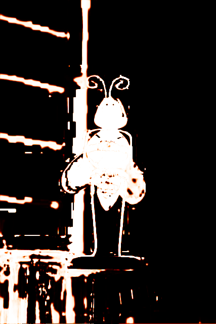
(c) FBP 2.

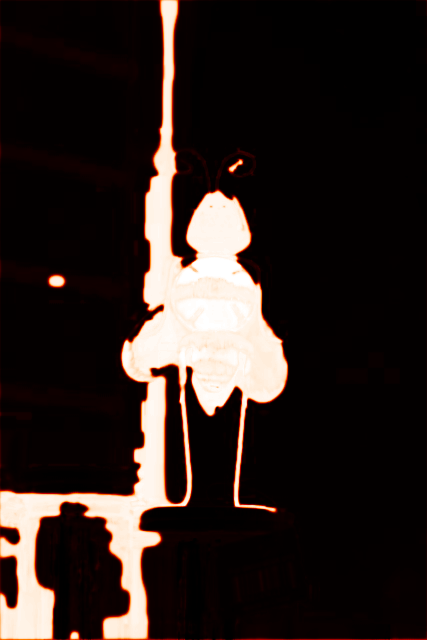
(d) FBP 3.

(e) FBP 4.

(f) HOP 1.

(g) Ground truth.

(h) DR 1.

(i) DR 2.

(j) DR 3.

(k) DR 4.

(l) HOP 2.

Figure 2: Example marginals from the different approximation procedures for the original image (a) with ground truth segmentation (g). For the results comparing FBP and DR (b-e,h-k) we have used the same pairwise weights and weights. The strength of the prior used monotonically decreases with the number specified after the respective method (i.e., b,f,h correspond to strong and e,k,l, to weak priors). Note how FBP is overconfident, whereas our method offers marginals with much higher dynamic range.

We now report experimental results on applying our parallel variational inference scheme to a challenging image segmentation problem as motivated in §2. The goal of our experiments is to test the scalability of our approach to large problems, and to evaluate the quality of the marginals both qualitatively and quantitatively. We used the data from Jegelka & Bilmes (2011), which contains a total of 36 images, each with a highly detailed (pixel-level precision) ground truth segmentation. Due to intractability, we cannot compute the exact marginals against which we would ideally wish to compare. As a proxy for measuring the quality of the approximations, we use the area under the ROC curve (AUC) as compared to the ground truth segmentation. We classify each pixel independently as fore- or background by comparing its approximate marginal against a threshold, which we vary to obtain the ROC curve. We have used the following model, which contains both pairwise and higher-order interactions.

$$F(A)=\alpha m(A)+\beta F_{\textrm{cut}}(A)+\gamma\sum_{P_{i}\in\mathcal{P}}\phi\left(\frac{|A\cap P_{i}|}{|P_{i}|}\right),$$

where

• the unary potentials $m(\cdot)$ were learned from labeled data using a 5 component GMM;

• the pairwise potentials $F_{\textrm{cut}}$ connect neighboring pixels $\mathbf{x}$ and $\mathbf{x}^{\prime}$ with weights $w(\mathbf{x},\mathbf{x}^{\prime})=\exp(-\theta\|\mathbf{x}-\mathbf{x}\|^{2})$, where $\mathbf{x}$ and $\mathbf{x}^{\prime}$ are the RGB values of the pixels;

• the higher order potentials were generated using the mean-shift algorithm of Comaniciu & Meer (2002). We have used two overlapping layers of superpixels, each layer with different granularity. The concave function was defined as $\phi(z)=z(1-z)$.

We compared the following inference techniques. The reported typical running times are for an image of size 427x640 pixels on a quad core machine and we report the wall clock time of the inference code (without setting up the factor graph or generating the superpixels).

• Unary potentials only with independent predictions, i.e., $\beta=\gamma=0$.

• Belief propagation (BP), mean-field (MF) and fractional belief propagation (FBP) for the pairwise model (i.e. $\gamma=0$). We have used the implementation from libDAI (Mooij, 2010). The maximum number of iterations was set to 30. We note that this code is not parallelized. When we observe fast convergence, for example BP can converge in 3 iterations, it takes about 45 seconds. Even though we have set a relatively low number of iterations, the running times can be extremely slow if the methods do not converge. For example, running mean-field for 30 iterations can take more than 3 minutes.

• Our approach using only pairwise potentials ($\gamma=0$), solved using the total variation Douglas-Rachford (DR) code from (Barbero & Sra, 2011, 2014; Jegelka et al., 2013). We ran for at most 100 iterations. The inference takes typically less than a second.

• Our approach with higher order potentials (HOP) only $(\beta=0)$. The inference takes less than 12 seconds.

For every method we tested several variants using different combinations for $\alpha,\beta,\gamma$ and $\theta$ (exact numbers provided in the appendix). Then, we performed a leave-one-out cross-validation for estimating the average AUC. We have also generated a sequence of 10 trimaps by growing the boundary around the true foreground to estimate accuracy over the hardest pixels, namely those at the boundary.

Method	Avg. AUC	Std. Dev.	Avg. AUCT	Std. Dev.
hop	0.9638	0.0596	0.9567	0.0642
dr	0.9602	0.0617	0.9496	0.0691
fbp	0.9500	0.0662	0.9357	0.0975
mf	0.9486	0.0675	0.9420	0.0764
unary	0.9484	0.0681	0.9425	0.0759
bp	0.9445	0.0779	0.9360	0.0964

Figure 3: Average scores of the methods estimated using leave-one-out cross validation. The Avg. AUC column is the average area under the ROC curve. The Avg. AUCT column reports the average of the mean AUC over the 10 trimaps. The second and the fourth columns are the standard deviation of the preceding columns.

(a) Average ROC curves for the different methods.

(b) Average AUC for trimaps of increasing size.

Figure 4: Comparison of inference methods in terms of their accuracy. For each method we optimize the parameters via grid-search, and report leave-one-out cross-validation results. (a) ROC curves for classifying pixels as fore- or background by independently thresholding marginals, averaged over the whole image. (b) Results over the trimaps (blurred boundaries around the ground truth segmentation), focusing on “difficult” pixels. For every algorithm and every of the 10 trimap sizes we report the average area under the curve.

Accuracy.

We first wish to quantitatively compare the accuracy of the approximate marginals. We report the aggregate results in Figure 3, and the ROC curves in Figure 4. We can clearly see that our approach outperforms the traditional inference methods for both objectives — the AUC over the whole image and over the challenging boundary (trimaps). Sometimes we see very poor behavior of the alternative methods, which can be attributed to either their over-confidence (as verified below), or the fact that they optimize non-convex objectives and can fail to converge within the given number of iterations. Lastly, capturing high-order interactions leads to higher accuracy (in particular around the boundary) than pairwise potentials only.

Properties of marginals.

We would also like to understand the qualitative characteristics of the resulting marginals of our methods when compared with the traditional techniques. From the discussion on the divergence minimization in §5, we would expect the approximate marginals to avoid assigning low probabilities and rather prefer to err conservatively, i.e., on the side of causing false positives. On the other hand, it is known that the results of belief propagation are often over-confident. For this purpose, we provide a visual comparison in Figure 2. Namely, each of the four FBP/DR pairs are results using the respective algorithms for the same parameters of the model. We observe exactly what the theory predicts — the distribution obtained via L-Field is less concentrated around the object and mass is spread around more. The contrast is starkest on Figures 2 (b) and (h), where we use a very strong pairwise prior (high $\beta$). On Figures 2 (e) and (k) we have used a very weak pairwise prior (low $\beta$), and as expected the resulting marginals are mainly determined by the unary part and the choice of inference procedure does not make a difference. The results in the last column are from the higher order model, with two different values of $\gamma$ (the strength of the higher order potential). We can see that the resulting probabilities better preserve the boundaries of the object and the fine details, which is one of the main benefits of using these models.

8 Conclusion

We have addressed the problem of variational inference in log-supermodular distributions. In particular, building on the L-Field approach of Djolonga & Krause (2014), we established two natural, important interpretations of their method. First, we showed how L-Field can be reduced to solving the well-studied minimum norm point problem, making a wealth of tools from submodular optimization suddenly available for approximate Bayesian inference. Secondly, we showed that the factorized distributions returned by L-Field minimize a particular type of information divergence. Both of these theoretical connections are immediately algorithmically useful. In particular, for the common case of decomposable models, both connections lead to efficient message passing algorithms. Exploiting the minimum norm connection, we proved strong convergence rates for a natural parallel approach, with convergence rates dependent on the factor graph structure. Lastly, we demonstrate our approach on a challenging image segmentation task. Our results demonstrate the accuracy of our marginals (in terms of AUC score) compared to those produced by classical techniques like belief propagation, mean field and variants, on models where these can be applied. We also show that performance can be further improved by moving to high-order potentials, leading to models where classical marginal inference techniques become intractable. We believe our results provide an important step towards practical, efficient inference in models with complex, high-order variable interactions.

Appendix A Theory

A.1 Equivalence between the minimum norm and inference problems

We will show a stronger result from which Theorem 2 follows by taking $w_{i}=1$ and $y_{i}=0$.

Lemma 3.

For positive weights $w_{i}>0$ the objectives $\sum_{i\in V}w_{i}(x_{i}-y_{i})^{2}$ and $\sum_{i\in V}\frac{1}{w_{i}}\log(\exp(-w_{i}x_{i})+\exp(-w_{i}y_{i}))$ have the same optimum under the constraint $\mathbf{x}\in B(F)$.

Proof.

For the second objective we have that

$$\sum_{i\in V}\frac{1}{w_{i}}\log(\exp(-w_{i}x_{i})+\exp(-w_{i}y_{i}))\stackrel{{\scriptstyle\mathbf{z}=-\mathbf{x}}}{{=}}\sum_{i\in V}\frac{1}{w_{i}}\log(\exp(w_{i}z_{i})+\exp(-w_{i}y_{i})).$$

Hence, the optimum of the problem is the negative of the problem on $-B(F)$, which is the base polytope of the submodular function $\overline{F}(A)=F(V-A)-F(V)$. The gradient of this objective with respect to any $z_{i}$ is equal to $\sigma(w_{i}(z_{i}+y_{i}))$, where $\sigma(u)=1/(1+e^{-u})$ is the sigmoid function. As the weights $w_{i}$ are positive, we have that

$$\sigma(w_{i}(z_{i}+y_{i}))\leq\sigma(w_{j}(z_{j}+y_{j}))\iff w_{i}(z_{i}+y_{i})\leq w_{j}(z_{j}+y_{j}).$$

From Fujishige (2005)[Theorem 8.1], it follows that the above problem and $\sum_{i}w_{i}(z_{i}+y_{i})^{2}$ have the same solution $\mathbf{z}^{*}$ on $-B(F)=B(\overline{F})$. However, if $\mathbf{z}^{*}$ is the projection of $-\mathbf{y}$ onto $-B(F)$, then $\mathbf{x}=-\mathbf{z}^{*}$ is the projection of $\mathbf{y}$ onto $B(F)$. ∎

A.2 Connection to the infinite Rényi divergences

If we expand the Rényi infinite divergence for $P(S)=\frac{1}{\mathcal{Z}_{p}}\exp(-F(S))$ and $Q(S)=\frac{1}{\mathcal{Z}_{q}}\exp(-q(S))$ for modular $q(\cdot)$ we get the following

$${D_{\infty}({P}\,\|\,{Q})}=\log\sup_{A\subseteq V}\frac{P(A)}{Q(A)}=\log\sup_{A\subseteq V}\frac{\exp(-F(A))/\mathcal{Z}_{p}}{\exp(-q(A))/\mathcal{Z}_{q}}=\log\mathcal{Z}_{q}-\log\mathcal{Z}_{p}+\sup_{A\subseteq V}\{q(A)-F(A)\}.$$ (7)

As we will consider the problem of minimizing the above quantity with respect to the modular function $q$ we can ignore the constant $\log\mathcal{Z}_{p}$. We will also expand the log-partition function of $q$, $\log\mathcal{Z}_{q}=\sum_{i\in V}\log(1+\exp(-q_{i}))$ and introduce a new variable $t$ capturing the supremum above to arrive at the following formulation.

$$\begin{split}\textrm{minimize}&\sum_{i\in V}\log(1+\exp(-q_{i}))+t\\ \textrm{subject to}&\quad q(A)\leq F(A)+t\quad\textrm{for all }A\subseteq V\end{split}$$ (8)

Definition 4.

For any normalized submodular function $F$, define $\mathcal{L}^{*}(F)$ to be the optimum value of minimizing $\sum_{i\in V}\log(1+\exp(-s_{i}))$ subject to $\mathbf{s}\in B(F)$.

To show the connection, we will need the following two lemmas.

Lemma 4 (Djolonga & Krause (2014)).

By strong Fenchel duality we have that

$$\mathcal{L}^{*}(F)=\min_{\mathbf{s}\in B(F)}\sum_{i\in V}\log(1+\exp(-s_{i}))=\sup_{\mathbf{p}\in[0,1]^{V}}\mathbb{H}[\mathbf{p}]-f(\mathbf{p}),$$

where $f$ is the Lovász extension of $F$ and $\mathbb{H}[\mathbf{p}]$ is the entropy of a random vector of independent Bernoulli random variables.

The following lemma is already known, as such functions have been already used, but we prove it for completeness.

Lemma 5.

For any normalized submodular function $F:2^{V}\to\mathbb{R}$ define $F_{\beta}:2^{V}\to\mathbb{R}$ as follows.

$$F_{\beta}(S)=\begin{cases}0&\text{if }S=\emptyset\\ F(S)+\beta&\text{if }S\neq\emptyset\end{cases}$$

Then, $F_{\beta}$ is submodular, normalized and has Lovász extension $f_{\beta}(\mathbf{w})=f(\mathbf{w})+\beta\max_{i}w_{i}$.

Proof.

To show that $F$ is submodular we need to show that (see e.g. (Bach, 2013)[Prop. 2.3]) for any $A\subseteq V$ and any $j,k\in V-A$ we have that $F_{\beta}(A\cup\{k\})-F_{\beta}(A)\geq F_{\beta}(A\cup\{j,k\})-F_{\beta}(A\cup\{j\})$. If $A\neq\emptyset$, then the above inequality follows immediately from the submodularity of $F$. Otherwise, we have the inequality $F(\{k\})+\beta-F(\emptyset)\geq F(\{j,k\})-F(\{j\})$, which again easily follows from the submodularity of $F$ and the fact that $\beta\geq 0$. The Lovász extension of $F_{\beta}$ is defined as

$$f_{\beta}(w)=\sum_{k=1}^{|V|}w_{j_{k}}\big{(}F_{\beta}(\{j_{1},\ldots,j_{k}\})-F_{\beta}(\{j_{1},\ldots,j_{k-1}\})\big{)},$$

where the indices are chosen so that $w_{j_{1}}\geq w_{j_{2}}\geq\ldots\geq w_{j_{|V|}}$. Then, every term in the sum will be the same if we replace $F_{\beta}$ with $F$ (because $\beta$ will be added and subtracted), except for the first term when $k=1$. This term is equal to $w_{j_{1}}(F(\{j_{1}\})+\beta-F(\emptyset))$, and the result follows immediately as $w_{j_{1}}=\max_{i}w_{i}$. ∎

Lemma 6.

For submodular functions Problem (8) reaches the minimum for $t=0$.

Proof.

Define $\textsc{OPT}_{\beta}$ to be the optimum value of problem (8) for $t=\beta$. Note that $\textsc{OPT}_{\beta}=\mathcal{L}^{*}(F_{\beta})+\beta$. Then

$$\textsc{OPT}_{0}\stackrel{{\scriptstyle\mathrm{Lem.}\ref{lem:duality}}}{{=}}\mathbb{H}[\mathbf{p}]-f(\mathbf{p})\leq\mathbb{H}[\mathbf{p}]-f(\mathbf{p})+\beta\underbrace{(1-\max_{i}p_{i})}_{\geq 0}\stackrel{{\scriptstyle\mathrm{Lem.}\ref{lem:fbeta}}}{{=}}\mathbb{H}[\mathbf{p}]-f_{\beta}(\mathbf{p})+\beta\stackrel{{\scriptstyle\mathrm{Lem.}\ref{lem:duality}}}{{\leq}}\mathcal{L}^{*}(f_{\beta})+\beta=\textsc{OPT}_{\beta}.$$

∎

And this immediately implies Lemma 1 and Theorem 3. We will now prove Lemma 2 by giving a specific counterexample.

Lemma 7.

There is a supermodular function for which the minimum is achieved for some $t>0$.

Proof.

For $t=0$, the Lagrange dual problem of Problem (8) is

$$\begin{split}\textrm{maximize}&-\sum_{A\subseteq V}F(A)\lambda_{A}+\sum_{i\in V}h(\sum_{A\ni i}\lambda_{A})\\ \textrm{subject to}&\quad 0\leq\sum_{A\ni i}\lambda_{A}\leq 1\quad\textrm{for all }i\in V,\\ \end{split}$$ (9)

where $h(p)=-p\log p-(1-p)\log(1-p)$ is the binary entropy function (defined so that $h(0)=h(1)=0$). The Lagrange dual is easily derived if we note that $-h(-u)$ is the covex conjugate of the primal objective and use (Boyd & Vandenberghe, 2004)[§5.1.6]. Consider the function

$$F(\emptyset)=0,F(\{1\})=-20,F(\{2\})=-8,F(\{1,2\})=-16,$$

which is supermodular as

$$F(1\mid\{2\}) =-16-(-8)=-8>-20=F(\{1\}),\textrm{ and}$$

$$F(2\mid\{1\}) =-16-(-20)=4>8=F(\{2\}).$$

For $t=1$ consider the primal feasible variable $x=(-19,-7)$, which has an objective value $<27.1$. For $t=0$ take the dual variable $\lambda_{\emptyset}=\lambda_{V}=0,\lambda_{1}=1=\lambda_{2}=1$, with a value of $-F(1)\lambda_{1}-F(0)\lambda_{0}+0=28>27.1$ and thus a strictly better value is achieved for $t=1$. ∎

Appendix B Proofs for Section 6

We will first define a dual formulation of the minimization problem, for which the claimed message passing scheme does BCD. We will work with the set of all valid Lagrange multipliers $\Lambda=\{\lambda\in\mathbb{R}^{\sum_{i=1}^{R}|V_{i}|}\colon(\forall v\in V)\>\sum_{i\in\delta(v)}\lambda_{v,i}=0\}$ and the product of base polytopes $\mathcal{B}=\otimes_{i=1}^{R}B(F_{i})$. For any element $\mathbf{y}$ of either of these sets we will denote by $y_{i,v}$ the coordinate corresponding to variable $v\in V_{i}$ of the $i$-th block ($1\leq i\leq R$). Moreover, for any vector $\mathbf{x}\in\mathbb{R}^{V}$ we will denote by $\mathbf{x}|_{S}$ its restriction to the coordinates $S\subseteq V$.

Theorem 5 (Following (Jegelka et al., 2013)).

The dual problem of

$$\textrm{minimize}_{\mathbf{x}}f(\mathbf{x})+\frac{1}{2}\|\mathbf{x}\|^{2}=\textrm{minimize}_{\mathbf{x}}\sum_{i=1}^{R}(f(\mathbf{x}|_{V_{i}})+\frac{1}{2}\|\mathbf{x}|_{V_{i}}\|_{G}^{2})$$ (10)

is equal to

$$\underset{\lambda\in\Lambda,\mathbf{y}_{i}\in B(F_{i})}{\textrm{maximize}}\sum_{i=1}^{R}-\frac{1}{2}\|\mathbf{y}_{i}-\lambda_{i}\|_{G*}^{2},$$ (11)

Proof.

The proof is based on that of (Jegelka et al., 2013)[Lemma 1]. The considered problem is the following.

$$\min_{\mathbf{x}}f(\mathbf{x})+\frac{1}{2}\|\mathbf{x}|_{2}^{2} =\min_{\mathbf{x}}\sum_{i=1}^{R}(f_{i}(\mathbf{x}_{V_{i}})+\frac{1}{2}\|\mathbf{x}_{V_{i}}\|_{G}^{2})\;\textrm{s.t.}\;\mathbf{x}_{V_{i}}=\mathbf{x}|_{V_{i}}$$

$$=\min_{\mathbf{x},\mathbf{x}_{V_{i}}}\max_{\lambda_{i}}\sum_{i=1}^{R}(f_{i}(\mathbf{x}_{V_{i}})+\frac{1}{2}\|\mathbf{x}_{V_{i}}\|_{G}^{2}-\lambda_{i}^{T}(\mathbf{x}_{V_{i}}-\mathbf{x}|_{V_{i}})).$$

Because we have zero duality gap, we can change the order of optimization. Then, if we optimize for $\mathbf{x}$, we see that the Lagrange multipliers have to belong to $\Lambda$, which was defined above. Hence, we have the following problem

$$\max_{\lambda\in\Lambda}\sum_{i}\min_{\mathbf{x}_{V_{i}}}\max_{\mathbf{y}_{i}\in B(F_{i})}(\mathbf{x}_{V_{i}}^{T}\mathbf{y}_{i}+\frac{1}{2}\|\mathbf{x}_{V_{i}}\|_{G}^{2}-\lambda_{i}^{T}\mathbf{x}_{V_{i}})=\max_{\lambda\in\Lambda}\sum_{i}\max_{\mathbf{y}_{i}\in B(F_{i})}\min_{\mathbf{x}_{V_{i}}}(\mathbf{x}_{V_{i}}^{T}\mathbf{y}_{i}+\frac{1}{2}\|\mathbf{x}_{V_{i}}\|_{G}^{2}-\lambda_{i}^{T}\mathbf{x}_{V_{i}}).$$

Consider the inner problem, i.e.

$$\operatorname{minimize}_{\mathbf{x}_{V_{i}}}\mathbf{x}_{V_{i}}^{T}\mathbf{y}_{i}+\frac{1}{2}\|\mathbf{x}_{V_{i}}\|_{G}^{2}-\lambda_{i}^{T}\mathbf{x}_{V_{i}}=\operatorname{minimize}_{\mathbf{x}_{V_{i}}}\mathbf{x}_{V_{i}}^{T}(\mathbf{y}_{i}-\lambda_{i})+\frac{1}{2}\|\mathbf{x}_{V_{i}}\|_{G}^{2},$$

which is exactly the negative of the convex conjugate of $\frac{1}{2}\|\cdot\|_{G}^{2}$ evaluated at $\lambda_{i}-\mathbf{y}_{i}$. Because the convex conjugate is equal to $\frac{1}{2}\|\cdot\|_{G*}^{2}$ (see e.g. (Boyd & Vandenberghe, 2004)[Ex. 3.22]), the above minimum is equal to $-\frac{1}{2}\|\mathbf{y}_{i}-\lambda_{i}\|_{G*}^{2}$, which we had to show.

∎

We can now easily see that the message passing algorithm is doing BCD for the dual — each node $F_{i}$ is first projecting to $\Lambda$ by subtracting the component-wise mean, and then clearly projecting onto $B(F_{i})$ under the norm defined in Definition 3.

We will now show the linear convergence rate. Because we consider the $k$-regular case, the primal can be written in the following simpler form

$$\underset{\mathbf{x}}{\operatorname{minimize}}\sum_{i=1}^{r}f(\mathbf{x}|_{V_{i}})+\frac{1}{2k}\|\mathbf{x}|_{V_{i}}\|^{2},$$

and the decomposed dual becomes the problem of finding the closest points between $\Lambda$ and $\mathcal{B}$

$$\underset{\lambda\in\Lambda,\mathbf{y}_{i}\in B(F_{i})}{\textrm{maximize}}\sum_{i}-\frac{k}{2}\|\mathbf{y}_{i}-\lambda_{i}\|^{2}.$$ (12)

We now use exactly the same argument as in (Nishihara et al., 2014)[§3.3] with some small changes necessary to accommodate our different definitions of $\Lambda$ and $\mathcal{B}$. Please refer to that paper and references therein for the terminology used in the remaining of the proof. We will show that the Friedrich’s angle between any two faces of $\mathcal{B}$ and $\Lambda$ is at most $\frac{2}{k^{2}|V|^{2}}$, which combined with (Nishihara et al., 2014)[Thm. 2 and Cor. 5] implies the theorem. To make the notation easier to parse, we will assume that the elements in $\mathcal{B}$ and $\Lambda$ are ordered so that first come the $|V_{1}|$ elements corresponding to $F_{1}$, then the $|V_{2}|$ elements corresponding to $F_{2}$ and so forth. Under this ordering, the vector space $\Lambda$ can be written as the nullspace of the following matrix

$$S=\frac{1}{\sqrt{k}}\bigg{(}\begin{array}[]{c|c|c}\underbrace{S_{1}}_{\in\mathbb{R}^{V\times V_{1}}}&\ldots&\underbrace{S_{R}}_{\in\mathbb{R}^{V\times V_{R}}}\end{array}\bigg{)},\text{where}\;[V_{i}]_{v,v^{\prime}}=[v=v^{\prime}].$$ (13)

As noted in (Nishihara et al., 2014), using (Bach, 2013)[Prop. 4.7] we can express the affine hull $\mathrm{aff}_{0}(\mathcal{B}_{z})$ of any face $\mathcal{B}_{z}$ as (where for each $i\in\{1,\ldots,R\}$ the sets $A_{r,1},\ldots,A_{r,M_{r}}$ form a partition of $V_{i}$)

$$\textrm{aff}_{0}(\mathcal{B}_{z})=\bigcap_{r=1}^{R}\bigcap_{m=1}^{M_{r}}\{(\mathbf{y}_{1},\ldots,\mathbf{y}_{R})\colon y_{r}(A_{r,1}\cup\ldots\cup A_{r,m})=0\},\textrm{where}\;\mathbf{y}_{i}\in B(F_{i}).$$

This set can be also written as the nullspace of the following matrix

$$T=\begin{pmatrix}\frac{\mathbf{1}^{T}_{A_{1,1}}}{\sqrt{|A_{1,1}|}}&&\\ \frac{\mathbf{1}^{T}_{A_{1,2}}}{\sqrt{|A_{1,2}|}}&&\\ \vdots&&\\ \frac{\mathbf{1}^{T}_{A_{1,M_{1}}}}{\sqrt{|A_{1,M_{1}}|}}&&\\ &\ddots&\\ &&\frac{\mathbf{1}^{T}_{A_{1,1}}}{\sqrt{|A_{R,1}|}}\\ &&\frac{\mathbf{1}^{T}_{A_{1,2}}}{\sqrt{|A_{R,2}|}}\\ &&\vdots\\ &&\frac{\mathbf{1}^{T}_{A_{1,M_{R}}}}{\sqrt{|A_{R,M_{R}}|}}\end{pmatrix}.$$

To compute the Friedrich’s angle we are interested in the singular values of $ST^{T}$ (Nishihara et al., 2014)[Lemma 6], which is equal to

$$ST^{T}=\frac{1}{\sqrt{k}}\bigg{(}\frac{\mathbf{1}_{A_{1,1}}}{\sqrt{|A_{1,1}|}},\ldots,\frac{\mathbf{1}_{1,M_{1}}}{\sqrt{|A_{1,M_{1}}|}},\ldots\frac{\mathbf{1}_{A_{R,1}}}{\sqrt{|A_{R,1}|}},\ldots,\frac{\mathbf{1}_{R,M_{R}}}{\sqrt{|A_{R,M_{R}}|}}\bigg{)}.$$

Hence, we have to analyze the eigenvalues of the square matrix $(ST^{T})^{T}(ST^{T})$, whose rows and columns are indexed by $\mathcal{I}=\{(r,m)\colon r\in[R],m\in[M_{r}]\}$, and whose $((r_{i},m_{i}),(r_{j},m_{j}))$ entry is

$$\frac{1}{k}\frac{|A_{r_{i},m_{i}}\cap A_{r_{j},m_{j}}|}{\sqrt{|A_{r_{i},m_{i}}||A_{r_{j},m_{j}}|}}.$$

We create a graph with vertices $\mathcal{I}$ and we add edges between distinct $(r_{i},m_{i})$ and $(r_{j},m_{j})$ with weight $|A_{r_{i},m_{i}}\cap A_{r_{j},m_{j}}|$ (zero weight means that we do not add that edge). The normalized graph Laplacian of this graph is equal to

$$[\mathcal{L}]_{(r_{i},m_{i}),(r_{j},m_{j})}=\begin{cases}1&\textrm{if }(r_{i},m_{i})=(r_{j},m_{j})\\ -\frac{1}{k-1}\frac{|A_{r_{i},m_{i}}\cap A_{r_{j},m_{j}}|}{\sqrt{|A_{r_{i},m_{i}}||A_{r_{j},m_{j}}|}}&\textrm{otherwise}.\end{cases}$$

Hence, $(ST^{T})^{T}(ST^{T})=I-\frac{k-1}{k}\mathcal{L}$. We want to lower-bound the Cheeger constant $h$ of this graph. Because the spectrum of a graph is the union of the spectra of the connected components we will assume that the graph is connected, as we can apply the same argument to every component. From the definition of $h$ we have that

$$h\geq 2\frac{\textrm{minimum cut}}{\textrm{volume}},\textrm{where}\;\textrm{volume}=\sum_{v\in V}|\delta(v)|(|\delta(v)|-1)=|V|(k^{2}-k).$$

What remains is to bound the minimum cut from below. Because the graph is connected, for any cut $U$ there must exist some $v$ that is in sets on both sides of the cut. Let $m$ be the number of sets in $U$ that contain it, and let $k-m$ be the number of sets in the complement that contain it. Then, the cut is of size is at least $m(k-m)\geq k-1$. Hence

$$h\geq 2\frac{k-1}{|V|(k^{2}-k)}=\frac{2}{|V|k}.$$

And by Cheeger’s inequality the smallest positive eigenvalue $\lambda_{2}$ of the Laplacian $\mathcal{L}$ is at least $\frac{2}{k^{2}|V|^{2}}$, which from the relationship $(ST^{T})^{T}(ST^{T})=I-\frac{k-1}{k}\mathcal{L}$ implies that the squared Friedrich’s angle $c_{F}^{2}$ between $\Lambda$ and $\mathcal{B}$ is at most

$$c_{F}^{2}\leq c_{F}=1-\frac{k-1}{k}\lambda_{2}\leq 1-\frac{1}{|V|^{2}k^{2}},$$

which completes the proof.

Appendix C Experiments

We have used the parameter values in the table below.

Parameter	Values
$\theta$	$0.1,0.001,0.0001$
$\alpha$	$1,0.1,0.01,0.001$
$\beta$	$10,1,0.1,0.01,0.001$
$\gamma$	$10,1,0.1,0.01,0.001$

References

- Bach (2010) Bach, Francis. Structured sparsity-inducing norms through submodular functions. In NIPS, 2010.
- Bach (2013) Bach, Francis. Learning with submodular functions: a convex optimization perspective. Foundations and Trends® in Machine Learning, 6(2-3), 2013.
- Barbero & Sra (2014) Barbero, Álvaro and Sra, Suvrit. Modular proximal optimization for multidimensional total-variation regularization. 2014.
- Barbero & Sra (2011) Barbero, Álvaro and Sra, Suvrit. Fast Newton-type methods for total variation regularization. In ICML, pp. 313–320, 2011.
- Boyd & Vandenberghe (2004) Boyd, Stephen P and Vandenberghe, Lieven. Convex Optimization. Cambridge University Press, 2004.
- Cevher & Krause (2011) Cevher, Volkan and Krause, Andreas. Greedy dictionary selection for sparse representation. IEEE Journal of Selected Topics in Signal Processing, 99(5):979–988, September 2011.
- Chakrabarty et al. (2014) Chakrabarty, Deeparnab, Jain, Prateek, and Kothari, Pravesh. Provable submodular minimization using Wolfe’s algorithm. In Advances in Neural Information Processing Systems, pp. 802–809, 2014.
- Comaniciu & Meer (2002) Comaniciu, Dorin and Meer, Peter. Mean shift: A robust approach toward feature space analysis. Pattern Analysis and Machine Intelligence, IEEE Transactions on, 24(5):603–619, 2002.
- Djolonga & Krause (2014) Djolonga, Josip and Krause, Andreas. From MAP to marginals: Variational inference in Bayesian submodular models. In Neural Information Processing Systems (NIPS), 2014.
- Edmonds (1970) Edmonds, Jack. Submodular functions, matroids, and certain polyhedra. Combinatorial structures and their applications, pp. 69–87, 1970.
- Fujishige (1980) Fujishige, Satoru. Lexicographically optimal base of a polymatroid with respect to a weight vector. Mathematics of Operations Research, 5(2):186–196, 1980.
- Fujishige (2005) Fujishige, Satoru. Submodular functions and optimization, volume 58 of Annals of Discrete Mathematics. 2005.
- Goldberg & Jerrum (2007) Goldberg, Leslie Ann and Jerrum, Mark. The complexity of ferromagnetic ising with local fields. Combinatorics, Probability and Computing, 16(01):43–61, 2007.
- Jegelka & Bilmes (2011) Jegelka, Stefanie and Bilmes, Jeff. Submodularity beyond submodular energies: coupling edges in graph cuts. In Computer Vision and Pattern Recognition (CVPR), 2011 IEEE Conference on, pp. 1897–1904, 2011.
- Jegelka et al. (2013) Jegelka, Stefanie, Bach, Francis, and Sra, Suvrit. Reflection methods for user-friendly submodular optimization. In NIPS, 2013.
- Jerrum & Sinclair (1993) Jerrum, Mark and Sinclair, Alistair. Polynomial-time approximation algorithms for the ising model. SIAM Journal on computing, 22(5):1087–1116, 1993.
- Kohli et al. (2009) Kohli, Pushmeet, Ladický, L’ubor, and Torr, Philip H.S. Robust higher order potentials for enforcing label consistency. International Journal of Computer Vision, 82(3):302–324, 2009.
- Krause & Guestrin (2005) Krause, Andreas and Guestrin, Carlos. Near-optimal nonmyopic value of information in graphical models. In Conference on Uncertainty in Artificial Intelligence (UAI), July 2005.
- Kulesza & Taskar (2012) Kulesza, A. and Taskar, B. Determinantal point processes for machine learning. Foundations and Trends in Machine Learning, 5(2–3), 2012.
- Minka et al. (2005) Minka, Tom et al. Divergence measures and message passing. Technical report, Technical report, Microsoft Research, 2005.
- Mooij (2010) Mooij, Joris M. libDAI: A free and open source C++ library for discrete approximate inference in graphical models. The Journal of Machine Learning Research, 11:2169–2173, 2010.
- Nagano & Aihara (2012) Nagano, Kiyohito and Aihara, Kazuyuki. Equivalence of convex minimization problems over base polytopes. Japan journal of industrial and applied mathematics, 29(3):519–534, 2012.
- Narasimhan et al. (2005) Narasimhan, Mukund, Jojic, Nebojsa, and Bilmes, Jeff. Q-clustering. In NIPS, volume 5, pp. 5, 2005.
- Nishihara et al. (2014) Nishihara, Robert, Jegelka, Stefanie, and Jordan, Michael I. On the convergence rate of decomposable submodular function minimization. In Advances in Neural Information Processing Systems, pp. 640–648, 2014.
- Orlin (2009) Orlin, James B. A faster strongly polynomial time algorithm for submodular function minimization. Mathematical Programming, 118(2):237–251, 2009.
- Pearl (1986) Pearl, Judea. Fusion, propagation, and structuring in belief networks. Artificial intelligence, 29(3):241–288, 1986.
- Pedregosa et al. (2011) Pedregosa, F., Varoquaux, G., Gramfort, A., Michel, V., Thirion, B., Grisel, O., Blondel, M., Prettenhofer, P., Weiss, R., Dubourg, V., Vanderplas, J., Passos, A., Cournapeau, D., Brucher, M., Perrot, M., and Duchesnay, E. Scikit-learn: Machine learning in Python. Journal of Machine Learning Research, 12:2825–2830, 2011.
- Rényi (1961) Rényi, Alfréd. On measures of entropy and information. In Fourth Berkeley symposium on mathematical statistics and probability, volume 1, pp. 547–561, 1961.
- Stobbe & Krause (2010) Stobbe, Peter and Krause, Andreas. Efficient minimization of decomposable submodular functions. In Proc. Neural Information Processing Systems (NIPS), 2010.
- Van Erven & Harremoës (2012) Van Erven, Tim and Harremoës, Peter. Rényi divergence and Kullback-Leibler divergence. arXiv preprint arXiv:1206.2459, 2012.
- Wainwright & Jordan (2008) Wainwright, Martin J. and Jordan, Michael I. Graphical models, exponential families, and variational inference. Found. Trends Mach. Learn., 1(1-2):1–305, 2008.