Scale Factor Self-Dual Cosmological Models

Abstract

We implement a conformal time scale factor duality for Friedmann-Robertson-Walker cosmological models, which is consistent with the weak energy condition. The requirement for self-duality determines the equations of state for a broad class of barotropic fluids. We study the example of a universe filled with two interacting fluids, presenting an accelerated and a decelerated period, with manifest UV/IR duality. The associated self-dual scalar field interaction turns out to coincide with the “radiation-like” modified Chaplygin gas models. We present an equivalent realization of them as gauged Kähler sigma models (minimally coupled to gravity) with very specific and interrelated Kähler- and super-potentials. Their applications in the description of hilltop inflation and also as quintessence models for the late universe are discussed.

1 Introduction

The physical phenomena occurring at different periods of the universe expansion are usually described by effective cosmological models, representing gravity coupled to scalar fields with appropriately chosen interactions specific for the energy scales in consideration. The increasing precision of the recent astrophysical data 2015arXiv150202114P ; 2015arXiv150201589P allows to further select a restricted number of favored shapes of the corresponding potentials Martin2013 , thus providing important hints in the search of dynamical symmetry principles governing the universe evolution Hooft:2014kq ; Kallosh:2013jk ; Kallosh:2014rz ; Ellis:2014lq ; Hinterbichler:2011hl . At extremely high energies, where no preferred scales exist, the conformal or Weyl symmetries completely determine the corresponding effective gravity-matter actions Kallosh:2010uo ; Kallosh:2002ph ; Kachru:2003jt ; Ferrara:2013fv ; Ferrara:2010zp . The description of lower densities and large scales phenomena, however, requires spontaneous or explicit breaking of the scale invariance Hooft:2014kq ; Kallosh:2013jk ; Kallosh:2014rz ; Hinterbichler:2011hl ; Csaki:2014dk . Hence an important problem to be addressed concerns the nature of the additional symmetries that might be responsible for the selection of very special combinations of interaction terms giving rise to scale non-invariant models with one of the favored inflaton or/and quintessence potentials Martin2013 ; Barreiro:2000mi ; Copeland:2006if ; Kamenshchik:2001ec ; Caldwell:1998wq ; Binetruy:1999qf ; Brax:1999ee .

In order to highlight the power of discrete symmetries (and of the physical principles behind them) in the derivation of the matter interactions, we consider a particular class of cosmological models manifesting discrete UV/IR symmetry that relate the short-distances and early-times behavior to that at large-distances and late-times. Although this symmetry should be broken at certain intermediate energy scales, it turns out to provide an effective description of the high energy features of the universe evolution in terms of the low energy ones. A few examples of such UV/IR-self-duality can be realized in selected cosmological models with two periods of decelerated/accelerated expansion, as for example in the $\Lambda$CDM model and its quintessence extensions Caldwell:1998wq ; Barreiro:2000mi ; Copeland:2006if ; Kamenshchik:2001ec . Our goal is to demonstrate that appropriate transformations of the metric and energy density, which keep invariant the critical scale ($L_{c}$) of the transition from radiation, matter or dark-matter (DM) dominated phase to the dark-energy (DE) one, act as a specific discrete on-shell Weyl symmetry of these models.

Since the early and the late Universe is approximately homogeneous and isotropic, i.e. $ds^{2}=a^{2}(\eta)[-d\eta^{2}+ds_{3}^{2}(k)]$, it is natural to expect that the desired UV/IR symmetries are related to the scale factor duality (SFD) transformations Veneziano91scalefactor ; Gasperini:2003sh ; Chimento:2003il ; Chimento:2008qq of the corresponding FRW equations. Our main result consists in the implementation of the conformal time scale factor duality in the way consistent with the weak energy condition. We also demonstrate that such SFD’s, when combined with time reflections, can be promoted to manifest UV/IR symmetries for a broad class of cosmological models. The requirement of self-duality allows us to fix the form of the matter self-interactions as well.

2 Conformal time Scale-Factor Duality

Let us introduce the following specific form of the conformal time SFD transformations of the scale factor $a(\eta)$, the energy density $\rho(a)$ and pressure $p(a)$ of the matter-fluid:

$$\tilde{a}(\eta)=\frac{c^{2}_{0}}{a(\eta)},\quad\quad\tilde{a}^{2}\tilde{\rho}(\tilde{a})=a^{2}\rho(a),\quad\quad\tilde{a}^{2}[3\tilde{p}(\tilde{a})+\tilde{\rho}(\tilde{a})]=-a^{2}[3p(a)+\rho(a)]$$ (1)

As one can easily check, they keep unchanged the form of the FRW equations

$$\kappa^{2}\rho=6\left(\frac{a^{\prime}}{a^{2}}\right)^{2}+\frac{6k}{a^{2}},\quad\quad\rho^{\prime}+3\frac{a^{\prime}}{a}(\rho+p)=0,$$

$$\kappa^{2}p=2\left(\frac{a^{\prime}}{a^{2}}\right)^{2}-\frac{4a^{\prime\prime}}{a^{3}}-\frac{2k}{a^{2}},\quad\quad\kappa^{2}=16\pi G,$$ (2)

(with $a^{\prime}=\frac{da}{d\eta}$, etc.) independently of the values of $k=0,\pm 1$, i.e. for spatially flat, open or closed universes. By construction, they are mapping expanding solutions of the original model to contracting ones of its dual, $\tilde{a}^{\prime}>0\mapsto{a}^{\prime}<0$, and vice-versa. However, one can use the invariance of eqs. (2) under time reflections

$$\eta\mapsto\tilde{\eta}\equiv 2\eta_{c}-\eta\ ,\quad a(\eta)\mapsto a(\tilde{\eta}),$$ (3)

which in composition with the scale factor duality (1),

$$\tilde{a}(\tilde{\eta})=\frac{c^{2}_{0}}{a(\eta)},$$ (4)

allows to relate two dual solutions both expanding or contracting, i.e. $a^{\prime}>0\mapsto\bar{a}^{\prime}>0$, etc. This particular form ensures that the critical time $\eta_{c}$, corresponding to the fixed point $\tilde{a}(\eta_{c})=a(\eta_{c})$, with $c_{0}^{2}=a(\eta_{c})^{2}$, remains invariant.

We next consider a few consequences of eqs. (1), representing the main features of the corresponding dual pairs of cosmological models in the case of fluids with generic equation of state (EoS), $p=\omega(\rho)\rho$ and $\tilde{p}=\tilde{\omega}(\tilde{\rho})\tilde{\rho}$.

Matter/DE duality: Since the deceleration parameters $q$ and $\tilde{q}$ have always opposite signs $q(\omega)=-\tilde{q}(\tilde{\omega})$, i.e.

$$\omega(\rho)+\tilde{\omega}(\tilde{\rho})=-\frac{2}{3},\quad q(\omega)=\frac{1}{2}[1+3\omega(\rho)][1+k\big{(}\frac{a}{a^{\prime}}\big{)}^{2}],$$ (5)

we realize that the entire radiation, matter or DM dominated phases of decelerated expansion are always mapped into the corresponding DE dominated accelerated expansion periods in the dual model. The fact that the transformations (1) give rise to such a matter/DE duality becomes evident in the case of perfect fluids with $\omega=const$. Then all the DE fluids $-1\leq\omega\leq-\frac{1}{3}$ are transformed into “matter-like” ones, with $-\frac{1}{3}\leq\omega\leq\frac{1}{3}$, and vice-versa. We have thus examples of pairs of dual Friedmann universes – e.g. the de Sitter universe ($\omega=-1$) is dual to the radiation filled universe ($\omega=1/3$), corresponding to the well known inverse proportionality relation between their scale factors,

$$a^{2}_{rad}(\eta)\sim\eta^{2}\;;\quad{\text{and}}\quad a_{dS}^{2}(\eta)\sim 1/\eta^{2}.$$

A dust dominated universe ($\omega=0$), with $\rho_{\omega=0}\sim 1/a^{3}$, is dual to cosmic domain-walls, $\rho_{\omega=-2/3}\sim 1/a$. The cosmic string gas, with $\omega_{str}=-\frac{1}{3}$, is dual to itself. Notice that outside the range of $-1\leq\omega\leq\frac{1}{3}$, the duality allows us to describe certain “phantom DE fluids”, with $-\frac{5}{3}\leq\omega<-1$, in terms of ordinary matter fluids with $\frac{1}{3}<\omega\leq 1$.

Weak energy condition’s consistency: An important property of the conformal time scale factor duality (1) is that it preserves the weak energy condition (WEC) for a broad variety of fluids. That is, if we require that the WEC ($p+\rho\geq 0$ and $\rho\geq 0$) is satisfied by both dual fluids, we find that the EoS parameters $\omega(\rho)$ and $\tilde{\omega}(\tilde{\rho})$ are restricted to the interval $[-1,1/3]$. This condition is not only fulfilled by all perfect fluids with constant $\omega$ such as dark energy, cold (dark) matter and radiation, but also by countless examples of dual models involving more complicated interacting multi-component fluids.

UV/IR duality: The scale factor inversions, independently of their cosmic Veneziano91scalefactor ; Gasperini:2003sh ; Chimento:2003il ; Chimento:2008qq or conformal time realizations, are always mapping the short distance scales (at certain fixed time $\eta$) in the original model to the large scales (at the same $\eta$) in the dual model and vice-versa. In the case of conformal time SFD’s (1), however, these relations are enhanced by an important new UV/IR ingredient. Namely, for WEC consistent fluids high energy densities $\rho$ and high scalar curvatures $R$ are always transformed to lower ones in the dual models. Perfect fluids, with $\rho_{\omega}=D_{\omega}a^{-3(1+\omega)}$ ($-1<\omega<\frac{1}{3}$) provide the simplest example of such UV/IR duality: their duals are again perfect fluids with $\tilde{\omega}=-\frac{2}{3}-\omega$ and $\tilde{\rho}=\rho^{\frac{3\omega-1}{3(\omega+1)}}$. The curvature transformation $\tilde{R}(R)$ turns out to be similar to that of $\tilde{\rho}(\rho)$, since as a consequence of eqs.(2) we have $R=\frac{\kappa^{2}}{2}(1-3\omega)\rho$. As expected, for the self-dual fluid, $\omega_{str}=-\frac{1}{3}$, we recover the proper inversion rule $\tilde{R}_{str}=\kappa^{4}/R_{str}$. Similar high/low densities and curvatures transformations take place for certain cosmological models involving two-component interacting $\omega(\rho)\neq const$ fluids considered in Sect.3 below.

Duality of event and particle horizons: As a consequence of the scale factor inversion followed by time reflection (4), the sign of the Hubble factor $H(a(\eta))=\frac{a^{\prime}}{a^{2}}$ is kept unchanged and its transformation law is given by $\tilde{a}\tilde{H}=aH$ (cf. eqs. (1)). This property allows us to demonstrate that scale factor duality maps a particle horizon in the original universe into a cosmological event horizon of its dual, and vice-versa. Take, for simplicity, flat, singular universes with scale factor in the range $(0,\infty)$. Then $r_{e}=\int_{a}^{\infty}\frac{da}{Ha^{2}}$ and $r_{p}=\int_{0}^{a}\frac{da}{Ha^{2}}$ are the comoving radii of event and particle horizons, respectively, and one can easily derive their duality transformations:

$$\tilde{r}_{p}=\int_{0}^{\tilde{a}}\frac{1}{\tilde{H}\tilde{a}}\;\frac{d\tilde{a}}{\tilde{a}}=-\int_{a(\tilde{a}=0)}^{a(\tilde{a})}\frac{1}{Ha}\frac{da}{a}=\int^{\infty}_{a}\frac{1}{Ha}\frac{da}{a}=r_{e},$$ (6)

while for the physical radii $L_{e}=ar_{e}$ and $L_{p}=ar_{p}$ we obtain:

$$\frac{L_{p}}{a}=\frac{\tilde{L}_{e}}{\tilde{a}}.$$ (7)

For $k\neq 0$ the same reasoning applies. Thus the dual of a universe possessing a particle horizon necessarily presents an event horizon, and vice-versa. This relates their causal structure: if the original universe has a space-like past infinity, its dual will have a space-like future infinity, while a null past infinity is dual to a null future infinity. Such is the case for matter fluids (presenting space-like past infinity and particle horizon) and DE fluids (presenting space-like future infinity and event horizons), in accordance with (5).

The scale factor duality, originally introduced as an extension of the superstring T-duality for time dependent cosmological backgrounds of dilaton gravity Veneziano91scalefactor ; Gasperini:2003sh , admits a few different cosmic and conformal time realizations, both in Einstein and in dilaton-axion gravities. It is known to be an essencial ingredient of the alternative models of dilaton driven pre-big-bang inflation. Its Einstein gravity cosmic time implementation has been used for the description of “phantom models” of dark energy Chimento:2003il ; Chimento:2008qq . Although our motivations to study the cosmological implications of the conformal time scale factor duality mainly concerns its applications as an UV/IR symmetry of the two phases of the post-inflationary evolution of the universe, we find worthwhile to briefly stand out the diferences and the similarities between the properties of these three families of scale factor dual cosmological models.

Cosmic time SFD in Einstein gravity: The cosmological models obtained by imposing the requirement of scale factor duality in cosmic time, $ds^{2}=-dt^{2}+a^{2}(t)ds_{3}^{2}(k=0)$,

$$\tilde{a}(t)=\frac{c^{2}_{0}}{a(t)},\quad\quad\tilde{\rho}_{cos}=\rho_{cos},\;\;\;\;\tilde{p}_{cos}=-p_{cos}-2\rho_{cos},\;\;\;\;\omega_{cos}+\tilde{\omega}_{cos}=-2,$$ (8)

studied in refs.Chimento:2003il ; Chimento:2008qq , manifest quite different features from the conformal time dual models considered in the present paper. The fact that the scale factor transformations leave unchanged the corresponding energy densities is the origin of an unavoidable presence of “phantoms” ($\tilde{\omega}_{cos}<-1$), as well as of the violation of the weak energy condition and, as a consequence, of their non-conventional UV/IR behavior.

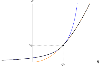
Figure 1: Self-dual solution obtained from the composition of two dual perfect fluids. The blue line represents $a_{\omega}(2\eta_{c}-\eta)$ for $\omega=-\tfrac{2}{3}$ (cosmic domain walls); the orange line represents its dual $a_{\tilde{\omega}}(\eta)$ for $\tilde{\omega}=0$ (dust). The black dashed line is the continuous, piecewise function $a(\eta)$, with $a(\eta)=a_{\omega}(2\eta_{c}-\eta)$ for $\eta\leq\eta_{c}$, and $a(\eta)=a_{\tilde{\omega}}(\eta)$ for $\eta\geq\eta_{c}$.

Dilaton gravity self-dual models: The original cosmic time scale factor duality transformations Veneziano91scalefactor ; Gasperini:2003sh ,

$$a(-t)=\frac{1}{a(t)},\quad\tilde{\varphi}=\varphi-6\ln a,\quad\tilde{\rho}_{dg}=a^{6}\rho_{dg},\;\;\;\;\tilde{p}_{dg}=-a^{6}p_{dg},\;\;\;\;\omega_{dg}+\tilde{\omega}_{dg}=0,$$ (9)

act as a discrete $Z_{2}\otimes Z_{2}$ symmetry of the homogeneous and isotropic solutions of dilaton gravity with a dilaton field $\varphi(t)$ coupled to specific (dual) matter fluids. As usual, the dilaton has a vanishing potential and the standard interaction with perfect fluids of density $\rho_{dg}$ and pressure $p_{dg}$, is assumed.

Despite the evident differences in the realizations of the corresponding cosmic and conformal time scale factor duality (1), (4) and (9), the problems addressed are quite similar: the construction of physically consistent self-dual solutions, presenting two phases (accelerated and decelerated) that are joined at the fixed points of time-reflection, $t_{c}$ or $\eta_{c}$. However, the presence or the absence of a dilaton allows for non-equivalent choices of the instants of acceleration/deceleration transition, and of different realizations of the dual or self-dual fluids, resulting in cosmological solutions with qualitatively different properties.

The simplest pre-big-bang cosmological solutions of dilaton gravity are obtained by considering a pair of perfect fluids, dual with respect to (9), one with accelerated and the other with decelerated expansions, “glued” together at $t=0$. The result is a self-dual cosmological model with a pre-big-bang inflationary phase in $t<0$ driven by a nontrivial dilaton $\varphi(t)$, and followed by the standard $\Lambda$CDM matter/radiation dominated period in $t>0$, with a constant dilaton. These models entail a curvature singularity and an infinite jump of the dilaton at the “big-bang” in $t=0$ Veneziano91scalefactor ; Gasperini:2003sh .

The conformal time Einstein gravity cosmological models obtained from (1) admit similar, but less singular and even completely non-singular, self-dual solutions, now in the Einstein frame. Indeed, a similar gluing procedure may be applied, e.g., to dual pairs of perfect fluids with $\omega\in(-1,1/3)$, related by (1). We join the scale factors at the point of time reflection $\eta_{c}$, when the dual scales coincide: $a(\eta_{c})=\tilde{a}(\eta_{c})=c_{0}$. The result, shown in fig.1, represents a simple two-phases universe evolution starting with a “big-bang” singularity (at $\eta=-\infty$), undergoing a phase of “inflationary” (i.e. accelerated) expansion up to $\eta_{c}$, when the deceleration period (driven by the dual fluid) begins. This composite solution is “almost smooth”, with only a finite jump of the deceleration parameter $q(a)$ and of the curvature at the joint at $\eta_{c}$. One can also construct physically more interesting universes presenting a completely smooth transition between the accelerated and decelerated phases. These models are based on a particular family of two interacting self-dual fluids with SFD invariant EoS derived in Sect.3, and further studied in Sect.5 below.

Our final remark concerns the common UV/IR features of the considered Einstein and dilaton gravity dual cosmological models. One can easily verify that eq.(9) give rise to a “density inversion law” $\tilde{\rho}_{dg}\propto\rho_{dg}^{\frac{\omega-1}{\omega+1}}$ for a pair of dual perfect fluids which shows that, similarly to the Einstein gravity conformal time dual models, also in dilaton gravity the high energy densities are mapped by scale factor duality (9) to low densities and vice versa.

3 Self-Dual Fluids

The properties established above provide a clear indication on how to convert the duality transformations (1) between pairs of dual cosmological models into an effective $Z_{2}\times Z_{2}$ symmetry of a single FRW solution by requiring its self-duality:

$$\tilde{a}(\eta)=a(\tilde{\eta}),\quad\quad\tilde{\rho}(\tilde{a})=\rho(\tilde{a}),\quad\quad\tilde{p}(\tilde{a})=p(\tilde{a}),$$ (10)

with $\tilde{\eta}=2\eta_{c}-\eta$ given by the time reflection (3). These constraints allow us to find the EoS for families of self-dual fluids, with $\tilde{\omega}(\tilde{\rho})=\omega(\tilde{\rho})$, as solutions to the functional equations

$$\frac{c_{0}^{2}}{a(\eta)}=a(2\eta_{c}-\eta),\quad\rho({\Omega}a)={\Omega}^{-2}\rho(a),\quad\omega(\rho)+\omega({\Omega}^{-2}\rho)=-\frac{2}{3},\quad\Omega\equiv\frac{c_{0}^{2}}{a^{2}}.$$ (11)

As suggested by the proper definition of the pairs of dual fluids with $\omega=const$, one possible solution is the sum of their densities,

$$\rho_{\omega}^{sd}(a)=Ba^{3\omega-1}+\tilde{B}a^{-3(1+\omega)},\quad\quad\tilde{B}=Bc_{0}^{2(1+3\omega)}.$$

With the addition of other pairs of dual fluids (and/or the self-dual fluid $\rho_{c}=\Omega_{c}a^{-2}$), one may construct more realistic models, as for example

$$\rho_{{\rm{\Lambda CDM}}}^{sd}=\Omega_{\Lambda}+\frac{\Omega_{rad}}{a^{4}}+\frac{\Omega_{dw}}{a}+\frac{\Omega_{dust}}{a^{3}}+\frac{\Omega_{c}}{a^{2}}.$$ (12)

This is nothing but the standard $\Lambda$CDM model enhanced by a new term, $\rho_{dw}=\Omega_{dw}/a$, representing cosmic domain walls with $\omega_{dw}=-2/3$. The fraction of the critical energy density due to this contribution is set fixed by the constraint of self-duality as

$$\Omega_{rad}/\Omega_{\Lambda}=(\Omega_{dust}/\Omega_{dw})^{2}=c_{0}^{4}.$$ (13)

The most general solution of the eqs. (11) for the energy density of a two-component self-dual fluid takes the form:

$$\rho=\Big{(}Ba^{-3(1+\beta)}+Da^{-3(1+\gamma)}\Big{)}^{\frac{4}{3(\gamma+\beta+2)}},$$ (14)

with $D=Bc_{0}^{3(\gamma-\beta)}>0,\ (\gamma+1)(\beta+1)\geq 0$. Its asymptotic behavior for small and large values of the scale factor is described by a family of dual pairs of perfect fluids with EoS parameters

$$\omega_{\gamma}=\frac{\gamma-3\beta-2}{3(\gamma+\beta+2)},\quad\quad\omega_{\beta}=\frac{\beta-3\gamma-2}{3(\gamma+\beta+2)},\quad\quad\omega_{\gamma}+\omega_{\beta}=-\frac{2}{3}.$$ (15)

Notice that all the self-dual fluids (14) satisfy the same “boundary” conditions: $\rho\to\{0\ {\text{or}}\ \infty\}$ when $a\to\{\infty\ {\text{or}}\ 0\}$, respectively. The exception is for $\beta=-1$, with an arbitrary $\gamma\equiv\frac{4}{3}\delta-1$. Then one of the asymptotic limits leads to a finite density, $\rho\to\rho_{dS}\equiv B^{\frac{1}{\delta}}$, and is a de Sitter universe with EoS parameter $\omega_{\beta}=-1$. On the opposite limit we find radiation, with $\omega_{\gamma}=1/3$. The self-dual fluid in this case is actually a modified Chaplygin gas Debnath:2004cq ; Benaoum:hh , with a rather simple EoS

$$\rho=\Big{(}B+Da^{-4\delta}\Big{)}^{\frac{1}{\delta}},\ \ \ p=\frac{1}{3}\rho-\frac{4}{3}B\rho^{1-\delta}.$$ (16)

The same approach can be used in the construction of more general self-dual energy densities, as for example,

$$\rho=\sum_{\alpha}\left(C_{\alpha}+E_{\alpha}a^{-r_{\alpha}}\right)^{p_{\alpha}}\left(B_{\alpha}+D_{\alpha}a^{-s_{\alpha}}\right)^{q_{\alpha}};\quad\quad r_{\alpha}p_{\alpha}+s_{\alpha}q_{\alpha}=4,$$ (17)

representing a composition of multiple different Chapligyn gas-like constituents. Each of the terms in the sum are separately self-dual given that their coefficients are related by

$$E_{\alpha}=c_{0}^{r_{\alpha}}\ C_{\alpha}\ ;\quad D_{\alpha}=c_{0}^{s_{\alpha}}\ B_{\alpha}\ .$$ (18)

Such combinations allow for richer phenomenological applications of self-dual models – but, on the other hand, they introduce many new free parameters and thus call for further physical requirements in order to select one (or a few) among the allowed densities.

In the following, we shall restrict ourselves to the study of the simplest two-fluids family of self-dual models (16). They permit a rather explicit analytic description, which makes evident the UV/IR nature of the corresponding conformal time SFD transformations (10) and (11). As we have already mentioned, the scale factor inversions always map the short distance scales into large distance ones in the dual model, and vice-versa Veneziano91scalefactor ; Gasperini:2003sh . This universal property is now complemented by the remarkably simple energy density and scalar curvature “inversion laws”:

$$\tilde{\rho}^{\delta}-\rho_{dS}^{\delta}=\frac{\rho_{dS}^{2\delta}}{\rho^{\delta}-\rho_{dS}^{\delta}},\quad\quad\quad\tilde{R}^{\tau}-R_{dS}^{\tau}=\frac{R_{dS}^{2\tau}}{R^{\tau}-R_{dS}^{\tau}},$$ (19)

with $\tau=\frac{\delta}{1-\delta}$. They are obtained by substitution of $a(\rho)$ from eq.(16) into the $\rho$ transformation law (11), i.e. in $\tilde{\rho}=\frac{a^{4}}{c_{0}^{4}}\rho$, and by taking into account the relation between curvatures and densities for the modified Chaplygin gas (16):

$$R=R_{dS}\left(\frac{\rho}{\rho_{dS}}\right)^{1-\delta},\quad\quad\quad R_{dS}=2\Lambda_{dS}=\frac{12}{L_{dS}^{2}}.$$ (20)

Hence, for the considered self-dual models with $\delta<1$, high densities and curvatures are transformed into small ones and vice-versa. The critical density $\rho_{c}\equiv\rho(\eta_{c})$, which marks the transition between decelerated and accelerated phases, is defined as a fixed point $\tilde{\rho}_{c}=\rho_{c}$ of the above transformation (19). With the help of the curvature radius $L^{2}\equiv 12/R$ transformation law

$$\tilde{L}^{\frac{2\delta}{1-\delta}}+L^{\frac{2\delta}{1-\delta}}=L_{dS}^{\frac{2\delta}{1-\delta}},$$ (21)

one can also calculate the “critical curvature scale” $L_{c}=\tilde{L}_{c}$ in terms of the (asymptotic) de Sitter radius: $L_{c}=2^{\frac{\delta-1}{2\delta}}L_{dS}$.

4 Reconstruction of the self-dual matter potentials

The requirements for scale factor duality of the FRW equations (2) can be also realized in an equivalent form by replacing the matter fluid with one scalar field $\sigma(\eta)$ with potential $V(\sigma)$, as usual:

$$\rho=\frac{1}{2}(\sigma^{\prime}/a)^{2}+V,\quad\quad\quad p=\frac{1}{2}(\sigma^{\prime}/a)^{2}-V,$$

where $\sigma^{\prime}=\frac{d\sigma}{d\eta}$. An efficient method for the explicit construction of self-dual scalar field potentials is provided by defining a superpotential ${\cal W}(\sigma)$ Cvetic:1995jo ; Cvetic:1997fx ; Townsend:2007ta ; Skenderis:2007yb and the related BPS-like first order equations:

$$a^{\prime 2}=\frac{a^{2}}{4}(\kappa^{2}a^{2}{\cal W}^{2}-4k),\quad\quad\sigma^{\prime 2}=-\frac{a^{3}}{2}\frac{d{\cal W}^{2}}{da},\quad\quad V(a)=\frac{3}{2}{\cal W}^{2}+\frac{a}{4}\frac{d{\cal W}^{2}}{da}.$$ (22)

In order to take advantage of the results already obtained in the case of fluids, we have substituted ${\cal W}(\sigma)$ and $V(\sigma)$ by ${\cal W}(a)=\sqrt{\frac{2}{3}\rho}$ and $V(a)$, taking into account the explicit expression of $a(\sigma)$. The corresponding scale factor self-duality transformations (11) now read

$${\cal W}(\Omega a)=\Omega^{-1}{\cal W}(a),\quad\tilde{\sigma}(\sigma)=\pm\int{\sqrt{\frac{2V-{\cal W}^{2}}{3{\cal W}^{2}-2V}}}d\sigma+\sigma_{0},$$

$$V(\Omega a)=-\Omega^{-2}\Big{(}V(a)-2{\cal W}^{2}(a)\Big{)},\quad\Omega\equiv\frac{c_{0}^{2}}{a^{2}}.$$ (23)

When applied to the example of the modified Chaplygin gas model (16) with $k=0$, the above equations give

$${\cal W}(\sigma)=\sqrt{\frac{2}{3}\rho_{dS}}\left(\cosh\left(\frac{\delta}{\sqrt{2}}\kappa(\sigma-\sigma_{0})\right)\right)^{\frac{1}{\delta}},\quad a(\sigma)=c_{0}\left(\sinh\left(\frac{\delta}{\sqrt{2}}\kappa(\sigma-\sigma_{0})\right)\right)^{-\frac{1}{2\delta}}$$ (24)

These results are sufficient to reproduce the self-dual potential:

$$V_{sd}(\sigma)=\frac{2}{\kappa^{2}L^{2}_{dS}}\Bigg{\{}\left[\cosh^{2}\left(\frac{\delta}{\sqrt{2}}\kappa(\sigma-\sigma_{0})\right)\right]^{\frac{1}{\delta}}+2\left[\cosh^{2}\left(\frac{\delta}{\sqrt{2}}\kappa(\sigma-\sigma_{0})\right)\right]^{\frac{1-\delta}{\delta}}\Bigg{\}},$$ (25)

and to derive the corresponding scalar field duality transformations as well:

$$\sinh\left(\frac{\delta}{\sqrt{2}}\kappa(\tilde{\sigma}-\tilde{\sigma}_{0})\right)\sinh\left(\frac{\delta}{\sqrt{2}}\kappa(\sigma-\sigma_{0})\right)=1.$$ (26)

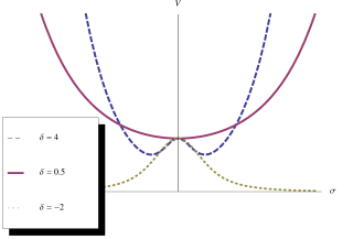
Figure 2: Self-dual potential (25) for different values of $\delta$. The de Sitter vacuum sits at $\sigma_{0}=0$.

Notice that the above non-linear $\tilde{\sigma}(\sigma)$ duality transformation is simply related to the scale factor inversions (1), i.e. $\tilde{a}(\tilde{\sigma})a(\sigma)=c_{0}^{2}$, and as expected it maps large $\sigma$ into small $\tilde{\sigma}$, and vice-versa.

The shape of the self-dual potential (25) depends crucially on the parameter $\delta$, as shown in fig.2. Models with $\delta>3/2$ present a double-well potential, with the maximum centered at $\sigma=\sigma_{0}$ (blue traced line). For $0<\delta\leq\frac{3}{2}$, the extremum $\sigma=\sigma_{0}$ is a global minimum (solid purple line), while for $\delta<0$ it becomes a global maximum (dotted yellow line). Such differences in shape reflect the allowed values of the effective mass $m^{2}_{\sigma}=V^{\prime\prime}(\sigma=\sigma_{0})$ of the scalar field $\sigma$, given by $L^{2}_{dS}m^{2}_{\sigma}=4\delta\left(\frac{3}{2}-\delta\right)$. As it is seen from eqs. (19) and (20), models with $\delta>1$ present a rather unphysical feature: the curvature of the universe increases with the deceasing of the matter density. We shall therefore exclude these models from the subsequent discussions.

5 UV/IR symmetric cosmological models

The eventual applications of the simplest family of self-dual models (25) (representing the modified Chaplygin gas (16), with $k=0$) in the description of the universe evolution require further investigation of the properties of their FRW’s solutions in order to establish for which values of the parameters $\delta$ and $L_{dS}$ they might be in agreement with the predictions of selected inflationary and/or $\Lambda$CDM-type models. The simple form of their energy density (16) allows to derive the exact solutions $\eta(a)$:

$$\eta\left(\frac{a}{c_{0}}\right)=\frac{aL_{dS}}{c^{2}_{0}}\ _{2}F_{1}\left(\frac{1}{2\delta},\frac{1}{4\delta};1+\frac{1}{4\delta};-\left(\frac{a}{c_{0}}\right)^{4\delta}\right),\quad c_{0}^{4\delta}=\frac{D}{B}=D\left(\frac{\kappa L_{dS}}{\sqrt{6}}\right)^{2\delta},$$ (27)

by direct integration of the first of eqs.(2). Their self-duality can be verified by taking into account the following identity between hypergeometric functions:

$$\eta(a/c_{0})=-\eta(c_{0}/a)+2\eta_{c},\quad\quad\eta_{c}=\frac{L_{dS}}{8\delta c_{0}}\frac{\left[\Gamma\left(\frac{1}{4\delta}\right)\right]^{2}}{\Gamma\left(\frac{1}{2\delta}\right)}.$$ (28)

[] []

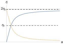
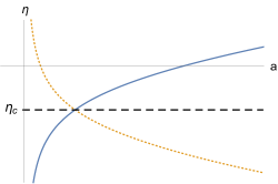
Figure 3: Conformal time as a function of scale factor, given by eq. (27). Blue lines represent $\eta(a/c_{0})$ and dotted orange lines, $\eta(c_{0}/a)$. (a) $\delta>0$; (b) $\delta<0$.

It can also be easily seen as the symmetry between the curves $\eta(a/c_{0})$ and $\eta(c_{0}/a)$ under a mirror reflection over the line $\eta_{c}$, as shown in fig.3. The geometric meaning of the self-duality condition, expressed in the first of the functional relations (11), is illustrated in fig.4: the blue curve gives the evolution of an universe as $\eta(a/c_{0})$; the pair of “dual” blue points have $\eta$-coordinates equidistant from the fixed point $\eta_{c}$. The scale-factor self-duality assures that the geometries at any such pair of blue points are related by a simple scale factor inversion – as it can be clearly seen with the help of the auxiliary orange curve $\eta(c_{0}/a)$.

Although the explicit form of the scale factor $a(\eta)$ can only be obtained in a few particular cases of $\delta=1,1/2,1/4$, the asymptotic behavior of $a(\eta)$ in the distant future and past of the universe may be read from the asymptotic limits of the hypergeometric function. The particular features depend crucially on the sign of $\delta$, i.e. on the shapes of the qualitatively different matter potentials (see fig.2).

In case $\delta>0$ – corresponding to the potential (25) indicated by the purple solid line in fig.2 – we realize that eq. (27) describes an expanding universe with singularity at $\eta=0$ and dominated by radiation, $a^{2}(\eta)\sim\eta^{2}$, at its initial decelerated phase. It ends, accelerated, as a de Sitter universe in the “far future”, when $a^{2}(\eta)\approx L_{dS}^{2}/(\eta_{f}-\eta)^{2}$, which shows that the end of its life is reached at finite conformal time $\eta_{f}=2\eta_{c}$ (see fig.3). Both the surfaces representing the singularity and future infinity are space-like, and therefore these universes present both particle and event horizons. If $L_{p}(\eta)$ is the physical radius of the particle horizon at an instant $\eta$ (necessarily in the decelerated period), then it relates to the physical radius $L_{e}(\tilde{\eta})$ of the event horizon at the instant $\tilde{\eta}=2\eta_{c}-\eta$ (necessarily in the accelerated period) through (cf. eq. (7))

$$L_{e}(\tilde{\eta})=\left(\frac{\tilde{L}}{L}\right)^{\frac{1}{1-\delta}}L_{p}(\eta),$$ (29)

where $L^{2}(\eta)\equiv 12/R(\eta)$ and $\tilde{L}^{2}\equiv 12/R(\tilde{\eta})$ are the Ricci curvature radius of space-time at each instant.

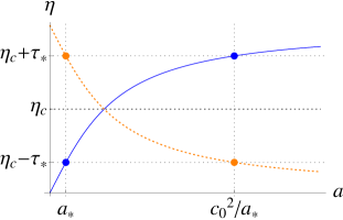
Figure 4: Geometric nature of self-duality. Blue curve is $\eta(a/c_{0})$, dotted orange curve is $\eta(c_{0}/a)$. The pairs of blue (and orange) points are related by a scale factor inversion.

The existence of both types of horizon was to be expected: as discussed in Sect.2, duality maps particle into event horizons and vice-versa, therefore a self-dual universe must possess either both types of horizon or none.

The solutions with $\delta<0$ – corresponding to the yellow dotted line in fig.2 – manifest quite different features, with monotonically decreasing and bounded density, $\rho_{dS}>\rho>0$, and curvature, $R_{dS}>R>0$, as it is clear form the fact that $V(\sigma)$ is always finite. Now, $\eta$ is defined on the entire real line, and thus we have an eternally expanding universe (see fig.3); here, past and future infinity are null hypersurfaces and there are neither particle nor event horizons, nor singularities. As one can see by taking $a\rightarrow 0$ in eq. (27), at the remote past ($\eta\rightarrow-\infty$) the space is asymptotically de Sitter, and is accelerated up to the moment $\eta_{c}$, when the decelerated phase begins. For large and positive $\eta$, in the far future, radiation dominates, with $a(\eta)^{2}\sim\eta^{2}$.

Let us consider in more detail the $\delta=\frac{1}{2}$ example, a self-dual fluid whose energy density

$$\rho(a)=\left(B+D\,a^{-2}\right)^{2}=\Omega_{\Lambda}+\frac{\Omega_{rad}}{a^{4}}+\frac{\Omega_{c}}{a^{2}}$$ (30)

is a sum of three interacting fluids: a cosmological constant with $\Omega_{\Lambda}=B^{2}$, radiation with $\Omega_{rad}=D^{2}$, and a cosmic string gas with $\Omega_{c}=2BD$. The EoS is $p=\frac{1}{3}\rho-\frac{4}{3}\sqrt{\Omega_{\Lambda}\rho}$. A particularly simple form of the $\eta(a)$ solution (27) then provides an explicit expression for the scale factor $a(\eta)$:

$$a(\eta)=c_{0}\tan\left(\frac{c_{0}}{L_{dS}}\eta\right),\quad 0<\eta<2\eta_{c}=\frac{L_{dS}}{c_{0}}\times\pi/2,\quad\frac{c_{0}}{L_{dS}}=\kappa\sqrt{\frac{\Omega_{c}}{12}},$$ (31)

The behavior near the singularity is readily seen by taking $\eta\ll 1$, so $a\sim\eta$, while the far future of the universe is attained in the limit $a\to\infty$, corresponding to the finite value of conformal time $\eta\to\eta_{f}=\frac{L_{dS}}{c_{0}}\times\pi/2=2\eta_{c}$. The simple form of $a(\eta)$ opens the opportunity to write this solution as a function of cosmic time as well:

$$a(t)=c_{0}\sqrt{e^{2L_{dS}t/c_{0}^{2}}-1},\quad\quad t=\int a(\eta)d\eta=-\frac{c_{0}^{2}}{L_{dS}}\log\left[\cos\left(\frac{L_{dS}}{c_{0}}\eta\right)\right].$$

We can also find the explicit transformation between the dual cosmic times. After calculating $\tilde{t}=\int\tilde{a}(\tilde{\eta})d\tilde{\eta}=-\int\frac{c_{0}^{2}}{a(\eta)}d\eta$, we easily find that $\tilde{t}(t)$ is given implicitly by

$$e^{-2L_{dS}\tilde{t}/c_{0}^{2}}=1-e^{-2L_{dS}t/c_{0}^{2}}.$$ (32)

We see that the conformal time scale factor duality (4) can be realized as a cosmic time scale factor inversion, $\tilde{a}(\tilde{t})=\frac{c^{2}_{0}}{a(t)}$, but with the rather nontrivial cosmic time transformation above.

The methods developed in the present paper were designed for the description of selected UV/IR symmetric cosmological models , representing two phases of decelerated and accelerated expansion. The above analysis of the FRW solutions of the simplest self-dual models (25), however, indicates two distinct physical regimes that can be asymptotically described by them:

Post-inflationary cosmology: The models with $0<\delta\leq 1$ (purple solid line in fig.2) possess features specific for the standard model post-inflationary cosmology. We have already seen in eq. (30) that the case $\delta=\frac{1}{2}$ corresponds to a combination of radiation, dark energy and a string gas, but without dust. For $\delta=\frac{1}{4}$ we now have all the elements of the self-dual version of $\Lambda$CDM shown in eq. (12):

$$\rho=\left(B+Da^{-1}\right)^{4}=\Omega_{\Lambda}+\frac{\Omega_{rad}}{a^{4}}+\frac{\Omega_{dw}}{a}+\frac{\Omega_{dust}}{a^{3}}+\frac{\Omega_{c}}{a^{2}},$$

with a specific relation between the critical densities

$$\Omega_{dust}=4BD^{3},\quad\Omega_{dw}=4DB^{3},\quad\Omega_{c}=6B^{2}D^{2},\quad\Omega_{rad}=D^{4},\quad\Omega_{\Lambda}=B^{4}.$$

Modifications of $\Lambda$CDM can also be found. For example, the self-dual potential with $\delta=3/4$ manifests many of the properties of the Chaplygin-like quintessence models Kamenshchik:2001ec ; Debnath:2004cq ; Benaoum:hh ; Chimento:kq . The energy density, which at early times is approximated by radiation, $\rho\approx\Omega_{rad}/a^{4}$, at relatively late times gets a contribution from the cosmological constant and dust, $\rho\approx\rho_{dS}+\Omega_{dm}/a^{3}$.

Hilltop inflation: On the other hand, the models with $\delta<0$ (yellow dotted line in fig.2) provide a realization of hilltop inflation Boubekeur:2005sw . The self-dual potential (25), nearby the “unstable” de Sitter vacuum at $\sigma=0$, take a form $V(\sigma)\approx 1-|\delta|\sigma^{2}$. Inflation takes place as the field rolls down this maximum, and ends when the field reaches the Planck scale, with $\sigma_{end}\sim m_{Pl}\equiv 1$. We may then calculate the number of e-foldings before the end of inflation

$$N(\sigma)=-\frac{1}{2|\delta|}\int_{1}^{\sigma}\frac{d\sigma^{\prime}}{\sigma^{\prime}},$$

and parametrize the field as $\sigma=e^{-2|\delta|N}$. The spectral index $n_{s}$ and the tensor-to-scalar ratio $r$, are then

$$n_{s}=1-4|\delta|-12\delta^{2}e^{-4|\delta|N},\quad r=32\delta^{2}e^{-8|\delta|N}.$$

Setting $N=60$ at the moment of horizon crossing and taking $\delta\approx-0.075$, we find $n_{s}\approx 1+4\delta\approx 0.97$, and $r\sim 10^{-5}$, which are in good agreement with the recent Planck2015 data 2015arXiv150201589P ; 2015arXiv150202114P .

As we have mentioned, more realistic inflationary and quintessence models (or even generalizations of $\Lambda$CDM) can be constructed when self-dual fluids with a more general EoS or with more components are considered, as in the examples given by eqs. (12), (14) and (17). Although they have not an explicit scalar field representation and require specific relations between the values of the critical densities of the constituent fluids, their advantage is to offer an equivalent description of the early time short distances physics in terms of the late time large distances one, guaranteed by scale-factor self-duality.

6 Concluding remarks

The most intriguing result of our study of the conformal time scale factor self-duality transformations is their “almost Weyl” form, seen in eqs. (11) and (23), as rescalings of the metric, superpotential, etc. – but with the exception of the matter field transformations (26). The question arrises of whether one can find an equivalent form of the considered models where the new matter field obeys a standard Weyl transformation. We begin with the encouraging observation that by a simple change of the field variable $\phi^{2}=\Phi\bar{\Phi}=6\tanh^{2}(\delta\sigma)$ (with $\kappa^{2}=2$) our self-dual models (25) are transformed into $SU(1,1)/U(1)$ Kähler sigma models, with gauge fixed $U(1)$ symmetry $\Phi=\bar{\Phi}=\phi$ and minimally coupled to Einstein gravity. Indeed such an embedding into ${\cal N}=1$ supergravity with one chiral matter supermultiplet is quite natural and expected due to its well known role in the construction of both quintessence Barreiro:2000mi ; Copeland:2006if ; Kamenshchik:2001ec ; Binetruy:1999qf ; Brax:1999ee and inflationary models Kallosh:2010uo ; Kallosh:2002ph ; Kachru:2003jt ; Kallosh:2014dw ; Ferrara:2013fv ; Ferrara:2010zp . The new feature, however, consists in a very special relation between the Kähler potential $K(\Phi,\bar{\Phi})$ and the superpotential $|{\cal Z}|={\cal W}(\phi)=e^{\frac{K}{2}}|W|$,

$$K=-\frac{1}{2\delta^{2}}\ln\Big{(}1-\frac{1}{6}\Phi\bar{\Phi}\Big{)},\quad|{\cal Z}|=\frac{\sqrt{2}}{L_{dS}}e^{\delta K},$$ (33)

where $W(\Phi)$ denotes the holomorphic superpotential of ${\cal N}=1$ Poincaré supergravity Kallosh:2014dw ; Cvetic:1995jo ; Cvetic:1997fx ; Townsend:2007ta ; Skenderis:2007yb . It is worthwhile to also mention that the inflationary $\alpha$-attractors Kallosh:2013jk ; Kallosh:2014rz , obtained within the superconformal supergravity approach Ferrara:2013fv ; Ferrara:2010zp , for a special choice of the inflaton potential:

$$f_{sd}^{2}\left(\frac{\phi}{\sqrt{6}}\right)=V_{sd}(\phi)=\frac{1}{9}\Big{(}\frac{6B}{6-\phi^{2}}\Big{)}^{\frac{1}{\delta}}(9-\phi^{2}),\ \alpha=\frac{1}{6\delta^{2}}$$

turns out to coincide with our model (25). There exists however an important difference between the well known “boundary” conditions for the $\alpha$-attractor potentials and those of our self-dual example, $f^{2}_{sd}(0)\neq 0$ and $f^{2}_{sd}(\pm 1)=\infty$ (for $\delta>0$), while for the attractors of ref. Kallosh:2013jk ; Kallosh:2014rz $f^{2}_{att}(0)=0$ and $f^{2}_{att}(1)={\rm{const.}}<\infty$. As a consequence, the vacua at the extremum $\phi=0$ represent different geometries: Minkowski for attractors and de Sitter for the self-dual potential (25), thus indicating that the supersymmetry is also broken on the latter.

With such a Kähler sigma model representation of the self-dual model (25), we may realize the conformal time SFD transformations (10) as a particular $Z_{2}$ Weyl transformation, now eqs. (1), (11) and (26) assuming a simple “linear form”:

$$\tilde{\phi}(\bar{\eta})=\Omega^{-\delta}\phi(\eta),\quad\quad\tilde{a}(\bar{\eta})=\Omega a(\eta),\quad\quad\Omega(\phi)=\Big{(}\frac{\phi^{2}}{6-\phi^{2}}\Big{)}^{\frac{1}{2\delta}}.$$ (34)

We should note these relations are valid on-shell – the knowledge of the explicit form of the scale factor $a(\sigma)$ as a function of the scalar field is needed in order to derive the $\tilde{\sigma}(\sigma)$ transformations (26), as well as their Weyl counterparts. The above form of the considered $Z_{2}\times Z_{2}$ symmetry also suggests an enlightening interpretation of the requirement for scale factor self-duality. It can be considered as an effective rescaling of the field $\phi$ and of the metric by a dynamically determined dilatation factor $\Omega(a_{*})>1$ at fixed time $\eta_{*}<\eta_{c}$, which when combined with the time reflection $\tilde{\eta}_{*}=2\eta_{c}-\eta_{*}$ ensures the equivalence of the short-distance physics at $\eta_{*}$ with the large-distance one at the “dual” instant $\tilde{\eta}_{*}$.

Our investigation of the self-duality aspects of the conformal time scale factor inversions has revealed they have an interesting new face as a UV/IR symmetry of a family of cosmological models manifesting two periods of expansion. As discussed in Sect.2, the problems we have addressed, although bearing some similarities, are not identical to the original dilaton gravity applications of the scale factor duality Veneziano91scalefactor ; Gasperini:2003sh . It is nevertheless worthwhile to mention that some of its most notable pre-big-bang features can be realized in our Einstein gravity cosmological models – one can construct a class of pre-big-bang-like self-dual solutions, despite the absence of the dilaton. This is achieved by taking an expanding solution of model (16) for $\delta>0$ (the blue curve in fig.3), and gluing it, at $\eta=0$, with its contracting image (the dotted orange line in fig. 3) obtained by the SFD inversion (1) together with a particular time translation, $\bar{\eta}=\eta-2\eta_{c}$. The result is a past-extended solution with an initial and a final accelerated periods (asymptotically de Sitter in the far future and past, $\eta\to\pm 2\eta_{c}$) separated by a decelerated phase in the middle of which (at $\eta=0$) there is a big-bang singularity. It is then natural to expect that the cosmological models we have studied might be identified as an Einstein frame version of certain pure dilaton gravity models (without any matter fluids), but with non-trivial potentials fixed by the self-duality requirement. This also suggests that some of the established self-duality properties may be observed in their Jordan frame realizations.

References

- (1) Planck Collaboration, P. A. R. Ade, N. Aghanim, M. Arnaud, F. Arroja, M. Ashdown, J. Aumont, C. Baccigalupi, M. Ballardini, A. J. Banday, and et al., Planck 2015. XX. Constraints on inflation, arXiv:1502.02114.
- (2) Planck Collaboration, P. A. R. Ade, N. Aghanim, M. Arnaud, M. Ashdown, J. Aumont, C. Baccigalupi, A. J. Banday, R. B. Barreiro, J. G. Bartlett, and et al., Planck 2015 results. XIII. Cosmological parameters, arXiv:1502.01589.
- (3) J. Martin, C. Ringeval, and V. Vennin, Encyclopædia Inflationaris, Physics of the Dark Universe 5 (Dec., 2014) 75–235.
- (4) G. T. Hooft, Local conformal symmetry: the missing symmetry component for space and time, 1410.6675.
- (5) R. Kallosh and A. Linde, Universality class in conformal inflation, JCAP 7 (July, 2013) 2.
- (6) R. Kallosh, A. Linde, and D. Roest, Large field inflation and double -attractors, JHEP 8 (Aug., 2014) 52.
- (7) J. Ellis, M. A. G. García, D. V. Nanopoulos, and K. A. Olive, A no-scale inflationary model to fit them all, JCAP 8 (Aug., 2014) 44.
- (8) K. Hinterbichler and J. Khoury, The pseudo-conformal universe: scale invariance from spontaneous breaking of conformal symmetry, JCAP 4 (Apr., 2012) 23.
- (9) R. Kallosh, A. Linde, and T. Rube, General inflaton potentials in supergravity, Phys.Rev.D 83 (Feb., 2011) 043507.
- (10) R. Kallosh, A. Linde, S. Prokushkin, and M. Shmakova, Supergravity, dark energy and the fate of the universe, Phys.Rev.D 66 (2002) 123503.
- (11) S. Kachru, R. Kallosh, A. Linde, and S. P. Trivedi, de sitter vacua in string theory, Phys.Rev.D 68 (2003) 046005.
- (12) S. Ferrara, R. Kallosh, A. Linde, and M. Porrati, Minimal supergravity models of inflation, Phys.Rev.D 88 (Oct., 2013) 085038.
- (13) S. Ferrara, R. Kallosh, A. Linde, A. Marrani, and A. Van Proeyen, Superconformal symmetry, NMSSM, and inflation, Phys.Rev.D 83 (Jan., 2011) 025008.
- (14) C. Csáki, N. Kaloper, J. Serra, and J. Terning, Inflation from Broken Scale Invariance, Phys.Rev.Lett. 113 (Oct., 2014) 161302.
- (15) T. Barreiro, E. J. Copeland, and N. J. Nunes, Quintessence arising from exponential potentials, Phys.Rev.D 61 (2000) 127301.
- (16) E. J. Copeland, M. Sami, and S. Tsujikawa, Dynamics of dark energy, Int.J.Mod.Phys.D 15 (2006) 1753–1936.
- (17) A. Y. Kamenshchik, U. Moschella, and V. Pasquier, An alternative to quintessence, Phys.Lett.B 511 (2001) 265–268.
- (18) R. R. Caldwell, R. Dave, and P. J. Steinhardt, Cosmological imprint of an energy component with general equation of state, Phys.Rev.Lett. 80 (1998) 1582–1585.
- (19) P. Binetruy, Models of dynamical supersymmetry breaking and quintessence, Phys.Rev.D 60 (1999) 063502.
- (20) P. Brax and J. Martin, Quintessence and supergravity, Phys.Lett.B 468 (1999) 40–45.
- (21) G. Veneziano, Scale factor duality for classical and quantum strings, Phys.Lett. 265 (1991) 265–287.
- (22) M. Gasperini and G. Veneziano, The pre-big bang scenario in string cosmology, Phys.Rept. 373 (2003) 1–212.
- (23) L. P. Chimento and R. Lazkoz, Constructing phantom cosmologies from standard scalar field universes, Phys.Rev.Lett. 91 (2003) 211301.
- (24) L. P. Chimento and W. Zimdahl, Duality invariance and cosmological dynamics, Int.J.Mod.Phys.D 17 (2008) 2229–2254.
- (25) U. Debnath, A. Banerjee, and S. Chakraborty, Role of modified chaplygin gas in accelerated universe, Class.Quant.Grav. 21 (2004) 5609–5618.
- (26) H. Benaoum, Accelerated universe from modified chaplygin gas and tachyonic fluid, hep-th/020.
- (27) M. Cvetic and H. H. Soleng, Naked singularities in dilatonic domain wall space-times, Phys.Rev.D 51 (1995) 5768–5784.
- (28) M. Cvetic and H. H. Soleng, Supergravity domain walls, Phys.Rept. 282 (1997) 159–223.
- (29) P. K. Townsend, From wave geometry to fake supergravity, Journal of Physics A Mathematical General 41 (Aug., 2008) D4014.
- (30) K. Skenderis, P. K. Townsend, and A. Van Proeyen, Domain-wall/cosmology correspondence in AdS/dS supergravity, JHEP 8 (Aug., 2007) 36.
- (31) J. Lu, D. Geng, L. Xu, Y. Wu, and M. Liu, Reduced modified Chaplygin gas cosmology, JHEP 1502 (2015) 071, [arXiv:1312.0779].
- (32) L. P. Chimento and R. Lazkoz, Large-scale inhomogeneities in modified Chaplygin gas cosmologies, Phys.Lett.B 615 (June, 2005) 146–152.
- (33) L. Boubekeur and D. H. Lyth, Hilltop inflation, JCAP 0507 (2005) 010.
- (34) R. Kallosh, Planck 2013 and superconformal symmetry, 1402.0527.