Methane depletion in both polar regions of Uranus inferred from HST/STIS and Keck/NIRC2 observations

Abstract

From Space Telescope Imaging Spectrograph (STIS) observations of Uranus in 2012, when good views of its north polar regions were available, we found that the methane volume mixing ratio declined from about 4% at low latitudes to about 2% at 60^∘ N and beyond. This depletion in the north polar region of Uranus in 2012 is similar in magnitude and depth to that found in the south polar regions in 2002. This similarity is remarkable because of the strikingly different appearance of clouds in the two polar regions: we have never seen any obvious signs of convective activity in the south polar region, while the north has been peppered with numerous small clouds thought to be of convective origin. Keck and Hubble Space Telescope imaging observations close to equinox at wavelengths of 1080 nm and 1290 nm, with different sensitivities to methane and hydrogen absorption but similar vertical contribution functions, imply that the depletions were simultaneously present in 2007, and at least their gross character is probably a persistent feature of the Uranus atmosphere. The depletion appears to be mainly restricted to the upper troposphere, with the depth increasing poleward from about 30^∘ N, reaching $\sim$4 bars at 45^∘ N and perhaps much deeper at 70^∘ N, where it is not well constrained by our observations. The latitudinal variations in degree and depth of the depletions are important constraints on models of meridional circulation. Our observations are qualitatively consistent with previously suggested circulation cells in which rising methane-rich gas at low latitudes is dried out by condensation and sedimentation of methane ice particles as the gas ascends to altitudes above the methane condensation level, then is transported to high latitudes, where it descends and brings down methane depleted gas. Since this cell would seem to inhibit formation of condensation clouds in regions where clouds are actually inferred from spectral modeling, it suggests that sparse localized convective events may be important in cloud formation. A more complex meridional circulation pattern may be necessary to reproduce the observed cloud distribution, but microwave observations appear to be most compatible with a single deep circulation cell. The small-scale latitudinal variations we found in the effective methane mixing ratio between 55^∘ N and 82^∘ N have significant inverse correlations with zonal mean latitudinal variations in cloud reflectivity in near-IR Keck images taken before and after the HST observations. If the CH₄ /H₂ absorption ratio variations are interpreted as local variations in para fraction instead of methane mixing ratio, we find that downwelling correlates with reduced cloud reflectivity. While there has been no significant secular change in the brightness of Uranus at continuum wavelengths between 2002 and 2012, there have been significant changes at wavelengths sensing methane and/or hydrogen absorption, with the southern hemisphere darkening considerably between 2002 and 2012, by $\sim$25% at mid latitudes near 827 nm, for example, while the northern hemisphere has brightened by $\sim$25% at mid latitudes at the same wavelength.

1. Introduction

Uranus experiences the solar system’s largest fractional seasonal forcing because its spin axis has a 98^∘ inclination to its orbital plane. It is thus not surprising to see a time-dependent north-south asymmetry in Uranus’ cloud structure. An especially interesting asymmetry noted by Sromovsky et al. (2012) is the continued complete absence of discrete cloud features south of 45^∘ S, while numerous discrete cloud features have been observed north of 45^∘ N in recent near-IR H-filter Keck images (Fig. 1). Voyager imaging in 1986 recorded no bright cloud features between the south pole and 45^∘ S. Nor were any seen in near-IR Hubble Space Telescope (HST) images taken with the Near-IR Camera and Multi-Object Spectrometer (NICMOS) beginning in 1997, nor in Keck images beginning in 2003. Some mechanism appears to be inhibiting convection at high southern latitudes that is not present at high northern latitudes. A very significant and possibly related result came from analysis of 2002 Space Telescope Imaging Spectrometer (STIS) observations by Karkoschka and Tomasko (2009), subsequently referenced as KT2009, and confirmed by the analysis of Sromovsky et al. (2011). They found a strong depletion of methane in the upper troposphere (down to a few bars at least) at high southern latitudes, suggesting a downwelling flow at these latitudes, which would tend to inhibit convective cloud formation. This raised the possibility of a connection between methane depletion and a lack of discrete cloud features, suggesting that high northern latitudes, where discrete clouds are seen, might not be depleted in methane. If so, the methane depletion might be a seasonal effect. In 2002, five years before equinox, the sub-observer latitude was 21.4^∘ S and the north polar region was not visible, so that testing this hypothesis would require new observations when the north polar region was exposed to view. We thus proposed new STIS observations of Uranus, which were obtained in late September 2012 (HST program 12894, Sromovsky, PI), five years after equinox, when the sub-observer latitude was 19.5^∘ N. The analysis of these new observations is the primary topic in what follows.

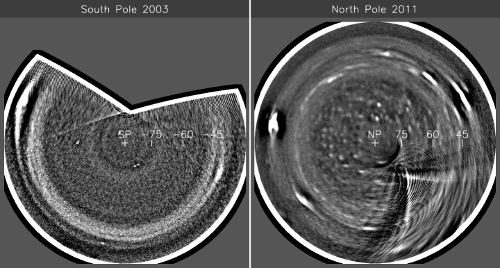
Figure 1.— Shift-and-add high-pass filtered projections of Uranus’ 2003 South (L) and 2011 North (R) polar regions reveal a large asymmetry in cloud features poleward of 45^∘, suggesting very different degrees of polar convection, a likely seasonal effect (Sromovsky et al. 2012). The images were obtained with the Keck 2 telescope and NIRC2 instrument using an H filter (1.62 $\mu$m central wavelength). The small bright features in the polar region in the 2011 image are 1-2% brighter than their surroundings. The features in the lower right quadrant of that image are heavily distorted by projection artificats.

Constraining the mixing ratio of CH₄ on Uranus is based on differences in the spectral absorption of CH₄ and H₂, illustrated by the penetration depth plot of Fig. 2A. Methane absorption dominates at most wavelengths, but hydrogen’s Collision Induced Absorption (CIA) is relatively more important in a narrow spectral range near 825 nm. Model calculations that don’t have the correct ratio of methane to hydrogen lead to a relative reflectivity mismatch near this wavelength. An example is shown in Fig. 2B-D, in which model calculations are compared to 2002 STIS observations assuming methane profiles with 2.2% and 4.0% deep volume mixing ratios. The two assumptions lead to very different errors in the vicinity of 825 nm, clearly indicating that the larger mixing ratio is a better choice. Karkoschka and Tomasko (2009) used this spectral constraint to infer a methane mixing ratio of 3.2% at low latitudes, but dropping to 1.4% at high southern latitudes. Sromovsky et al. (2011) analyzed the same data set, but used only temperature and mixing ratio profiles that were consistent with the Lindal et al. (1987) refractivity profiles. They confirmed the depletion but inferred a somewhat higher mixing ratio of 4% at low latitudes and found that better fits were obtained if the high latitude (down to $\sim$2-4 bars). Subsequently, 2009 groundbased spectral observations at the NASA Infrared Telescope Facility (IRTF) using the SpeX instrument, which provided coverage of the key 825-nm spectral region, were used by Tice et al. (2013) to infer that both polar regions were weakly depleted in methane, but they inferred lower methane mixing ratios, smaller latitudinal variations, and higher uncertainties than the STIS-based analysis of KT2009 and Sromovsky et al. (2011). These lower IRTF-based values might be a result of lower spatial resolution combined with worse view angles into the polar regions than obtained by HST observations.

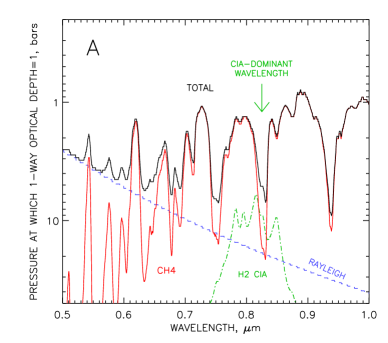
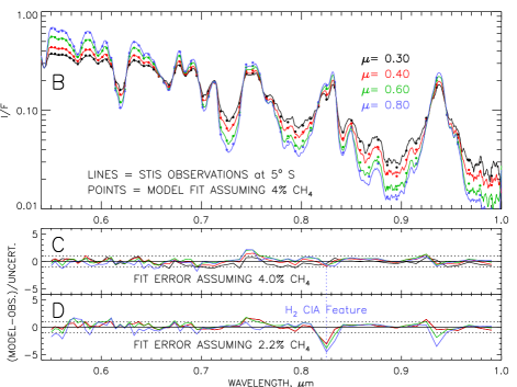
Figure 2.— A: Penetration depth vs. wavelength as limited by different opacity sources assuming the F1 methane profile and absorption models discussed in Sec. 6.1. Note the greater importance of H₂ CIA near 825 nm. The dark solid curve includes all absorbers, while the other curves are for single absorbers in isolation. B: Example model fit for the F1 profile of Sromovsky et al. (2011) with a deep methane volume mixing ratio of 4%, and fit errors for deep methane mixing ratios of 4% (C) and 2.2% (D). The fit errors near 825 nm are a sensitive indicator of the mixing ratio of CH₄ to H₂.

In the following we begin with a description of our 2012 HST/STIS observations, and the complex data reduction and calibration procedures. We then describe the relatively direct implications of latitudinal spectral variations and simplified model results. Finally, we describe our radiation transfer calculation methods and the results of constraining the cloud structure and methane distributions to fit the observed spectra. We show that the methane depletion is indeed present in both polar regions but of significantly different character. The results provide no obvious explanation for the asymmetry in polar cloud structure, but do raise some important questions about cloud formation. The important implications for meridional circulation models are discussed before summarizing our results.

2. Observations

Our 2012 observations used four HST orbits, three of them devoted to STIS spatial mosaics and one orbit to Wide Field Camera 3 (WFC3) support imaging. The STIS observations were taken on 27-28 September 2012 and the WFC3 observations on 30 September 2012. Observing conditions and exposures are summarized in Table 1.

Table 1Science exposures from HST program 12894. All STIS spectra used the 52^′′$\times$0.1^′′ slit.

	Start	Start	Instrument	Filter or	Exposure	No. of	Phase
Orbit	Date (UTH)	Time (UTH)		Grating	(sec)	Exp.	Angle (∘)
1	2012-09-27	21:22:29	STIS	MIRVIS	10.1	1	0.09
1	2012-09-27	21:38:11	STIS	G430L	70.0	13	0.09
2	2012-09-27	22:56:43	STIS	G750L	86.0	18	0.08
3	2012-09-28	00:32:26	STIS	G750L	86.0	18	0.08
4	2012-09-30	22:44:50	WFC3	F336W	30.0	1	0.09
4	2012-09-30	22:46:35	WFC3	F467M	16.0	1	0.09
4	2012-09-30	22:48:15	WFC3	F547M	6.0	1	0.09
4	2012-09-30	22:49:39	WFC3	F631N	65.0	1	0.09
4	2012-09-30	22:52:08	WFC3	F665N	52.0	1	0.09
4	2012-09-30	22:54:15	WFC3	F763M	26.0	1	0.09
4	2012-09-30	22:56:02	WFC3	F845M	35.0	1	0.09
4	2012-09-30	22:57:56	WFC3	F953N	250.0	1	0.09
4	2012-09-30	23:04:27	WFC3	FQ889N	450.0	1	0.09
4	2012-09-30	23:16:02	WFC3	FQ937N	160.0	1	0.09
4	2012-09-30	23:23:05	WFC3	FQ727N	240.0	1	0.09

On September 28 the sub-observer planetographic latitude was 19.5^∘ S, the observer range was 19.0613 AU (2.851530$\times$10⁹ km), and the equatorial angular diameter of Uranus was 3.6976 arcseconds.

2.1. STIS spatial mosaics.

STIS observations used the G430L and G750L gratings and the CCD detector, which has $\sim$0.05 arcsecond square pixels covering a nominal 52${}^{\prime\prime}\times$52^′′ square field of view (FOV) and a spectral range from $\sim$200 to 1030 nm (Hernandez et al. 2012). Using the 52${}^{\prime\prime}\times$0.1^′′ slit, the resolving power varies from 500 to 1000 over each wavelength range due to fixed wavelength dispersion of the gratings. Observations had to be carried out within a few days of Uranus opposition (29 September 2012) when the telescope roll angle could be set to orient the STIS slit parallel to the spin axis of Uranus.

One STIS orbit produced a mosaic of half of Uranus using the CCD detector, the G430L grating, and 52${}^{\prime\prime}\times$0.1^′′ slit. The G430L grating covers 290 to 570 nm with a 0.273 nm/pixel dispersion. The slit was aligned with Uranus’ rotational axis, and stepped from the evening limb to the central meridian in 0.152 arcsecond increments (because the planet has no high spatial resolution center-to-limb features at these wavelengths we used interpolation to fill in missing columns of the mosaic). Two additional STIS orbits were used to mosaic the planet with the G750L grating and 52${}^{\prime\prime}\times$0.1^′′ slit (524-1027 nm coverage with 0.492 nm/pixel dispersion), with limb to central meridian stepping at 0.0569 arcsecond intervals. This was the same procedure that was used successfully for HST program 9035 in 2002 (E. Karkoschka, P.I.). As Uranus’ equatorial radius was 1.85 arcseconds when observations were performed, stepping from one step off the limb to the central meridian required 13 positions for the G430L grating (at 0.152 arcseconds/step) and 36 for the G750L grating (at 0.0569 arcseconds/step). Two orbits were needed to complete the G750L grating observations, spanning a total time of 2 h 17 m, during which Uranus rotated 47^∘. This rotation was not a problem because of the high degree of zonal symmetry of Uranus and because our analysis rejected any small scale deviations from it, such as rare discrete cloud features.

Exposure times were similar to those used in the 2002 program, with 70-second exposures for G430L and 86-second exposures for G750L gratings, using the 1 electron/DN gain setting. These exposures yielded single-pixel signal-to-noise ratios of around 10:1 at 300 nm, $>$ 40:1 from around 400 to 700 nm, and decreasing to around 20:1 (methane windows) to $<$ 10:1 (methane absorption bands) at 1000 nm.

2.2. Supporting WFC3 imaging.

Since STIS images can be radiometrically calibrated for point sources or infinitely-extended sources, and Uranus is neither, an empirically determined correction function must be applied to the images as a function of wavelength. This function was determined for the 2002 STIS observations using WFPC2 images of Uranus taken around the same time as the 2002 STIS Uranus observations. To ensure that this function was determined as well as possible for the Cycle 20 observations in 2012, and to cross check the extensive spatial and spectral corrections that are required for STIS observations, we used one additional orbit of WFC3 imaging at a pixel scale of 0.04 arcseconds with eleven different filters spread over the 300-1000 nm range of the STIS spectra. These WFC3 images are displayed in Fig. 3, along with synthetic images with the same spectral weighting constructed from STIS spatially resolved spectra, as described in the following section. The filters and exposures are provided in Table 1.

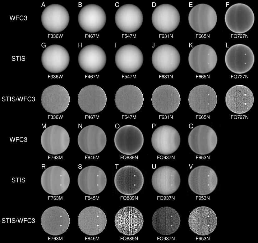
Figure 3.— WFC3 images of Uranus taken on 30 September 2012 (A-F and M-Q) compared to synthetic band-pass filter images (G-L and R-V) created from weighted averages of STIS spectral data cubes using WFC3 throughput and solar spectral weighting. The north pole is at at the right. Portions of the synthetic images east of the central meridian are obtained by reflection of the images west of the central meridian. That is why the single cloud feature appears twice in images where cloud contrast is sufficient to make the cloud visible. The STIS data were acquired three days before the WFC3 data, which were taken when the discrete cloud was not visible. The ratio images are stretched to make 0.8 black and 1.2 white. A direct comparison of latitude scans at fixed view angles is provided in the on-line analysis supplement file.

3. Data reduction and calibration.

The STIS pipeline processing used at STScI does not yield suitably calibrated two-dimensional spectral images for an object like Uranus. Considerable additional effort was required to reach a final calibration of these data, using techniques developed by KT2009 and closely followed in the calibration of the 2012 STIS observations. Flat-fielded science images, fringe flats, and WAVECALS from the STScI STIS data processing pipeline are the inputs to a rather extensive post-processing suite, each step of which is described in Section 1 of the on-line analysis supplemental file. (WAVECALS are exposures of arc sources used for wavelength calibration.) The output is a cube of geometrically and radiometrically calibrated monochromatic images of Uranus. However, this cube needs a final correction based on comparisons with the WFC3 support images.

Each WFC3 image was deconvolved with an appropriate Point-Spread Function (PSF) obtained from the Tiny Tim code of Krist (1995). To match the spatial resolution of the STIS images, the WFC3 images were then reconvolved with an approximation of the PSF given in the analysis supplemental file. They were then converted to I/F using header PHOTFLAM values and the Colina et al. (1996) solar flux spectrum, averaged over the WFC3 filter bandpasses. (The PHOTFLAM value is used to convert instrument DN/second to flux units.) To obtain a disk-averaged I/F, the planet’s light was integrated out to 1.1 equatorial radii and averaged over the planet’s cross section in pixels, computed using NAIF ephemerides (Acton 1996) and SPICELIB limb ellipse model (SPICELIB is NAIF toolkit software used in generating navigation and ancillary instrument information files.) The disk-averaged I/F was also computed for each of the STIS monochromatic images, and the filter- and solar flux-weighted I/F was computed for each of the WFC3 filter passbands that we used.

By comparing the uncalibrated STIS synthetic disk-averaged I/F to the corresponding WFC3 values, we constructed a correction function to radiometrically calibrate the STIS cube. Figure 4 shows the ratios of STIS to WFC3 disk-integrated brightnesses, and the quadratic function that we fit to these ratios as a function of wavelength. We weighted the filters by the square root of their band widths, and computed an effective wavelength weighted according to the product of the solar spectrum and the I/F spectrum of Uranus. The RMS deviation of individual filters from the calibration curve given in Fig. 4 is 3.7%, but only 0.94% when the FQ937N filter is omitted from the RMS calculation (but still included in the fit). While the FQ937N ratio deviates by 10% from the final calibration curve, it is not likely due to a problem with the filter calibration, as a comparison with the uranian satellite Ariel found it to be consistent with the other filters. More likely is that the darker parts of the STIS spectrum require slightly different calibrations than the brighter parts due to residual errors in Charge Transfer Efficiency (CTE) corrections (described in Section 1 of the analysis supplement file). Figure 4 also shows the function that was used to radiometrically calibrate the 2002 STIS data by KT2009. We do not know whether the difference in functions is due to a true STIS instrument change, to spatial variations across the CCD (2012 and 2002 observations were acquired at different locations on the CCD), or to a difference in filters used in the two calibrations (the 2002 data were calibrated using images taken by the Wide Field Planetary Camera 2 (WFPC2) instrument, the predecessor to WFC3).

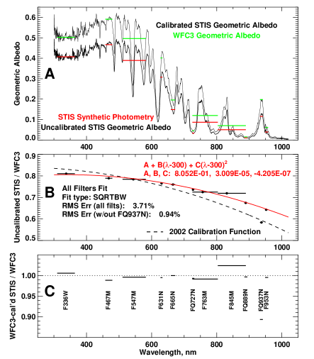
Figure 4.— A: Disk-integrated I/F spectra before final calibration (lower curve) and after final calibration (upper curve), where horizontal red bars indicate synthetic I/F values computed from pre-calibration spectra and horizontal green bars indicate I/F values obtained from WFC3 imaging. B: Synthetic band-pass filter disk-integrated I/F values (pre-calibration) divided by corresponding I/F values obtained from WFC3 measurements (horizontal bars). The red (solid) curve and legend coefficients defining it, were obtained by fitting all ratio values including that obtained from the FQ937N filter. The black (dashed) curve is the calibration function obtained from the 2002 data set. C: Ratio of synthetic disk-integrated I/F values obtained from calibrated STIS spectra to the corresponding WFC3 values.

As a sanity check on the STIS processing we compared line scans across WFC3 images to the corresponding scans across synthetic WFC3 images created from our calibrated STIS data cubes. These generally were in excellent agreement for $\mu$ values from 0.3 to 0.8, as demonstrated by plots given in Section 2 of the on-line analysis supplement file. The most significant discrepancy is in the overall I/F level computed for the FQ937N filter, a consequence of our calibration curve being 10% high for that filter. This can also be seen in the ratio images plotted in Fig. 3.

3.1. Center-to-limb fitting

Center-to-limb profiles provide important constraints on the vertical distribution of cloud particles as well as the vertical variation of methane compared to hydrogen. Because Uranus has a high degree of zonal uniformity, these profiles are fairly smooth functions that can be characterized by a small number of parameters, making it possible to constrain the profiles accurately, reducing the effects of noise and skipping over any small discrete cloud features. Because the observations were taken very close to zero phase angle these functions are almost perfectly symmetric about the central meridian, so that they depend on only one cosine value (observer and solar zenith angles are essentially equal). This is also one reason we were able to characterize these profiles by measuring only one half of the Uranus disk. These fits also facilitate the separation of latitudinal variations from those associated with view angle variations.

Before fitting the center-to-limb (CTL) profile for each wavelength, the spectral data are smoothed in the wavenumber domain to a resolution of 36 cm^-1, which equals the resolution we use in computing the Raman spectrum, but is four times finer than the sampling we use in constraining cloud models. The smoothing is helpful in reducing noise at longer wavelengths without degrading important spectral features. For each 1^∘ of latitude from 54^∘ S to 85^∘ N, all image samples within 1^∘ of the selected latitude and with $\mu>$ 0.175 are collected and fit to the empirical function

$$I(\mu)=a+b\mu+c/\mu,$$ (1)

assuming all samples were collected at the desired latitude and using the $\mu$ value for the center of each pixel of the image samples. Sample fits are provided in Fig. 5 and in Fig. 2 of the on-line supplement. Most of the scatter about the fitted profiles is due to noise, which is often amplified by the deconvolution process. Because the range of observed $\mu$ values decreases away from the equator at high southern and northern latitudes, we chose a moderate value of $\mu$=0.6 as the maximum view-angle cosine to provide a reasonably large unextrapolated range of 33.6^∘ S to 72.6^∘ N for 2012 observations and 74.5^∘ S to 31.7^∘ N for 2002. Unless otherwise noted all our results are derived without extrapolation.

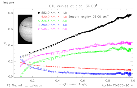
Figure 5.— Sample center-to-limb fits for 30^∘ N, as described in the main text. STIS I/F samples and fit lines with uncertainty bands are shown for five different wavelengths indicated in the legends. The latitude band sampled for these fits is darkened in the inset image of the half-disk of Uranus.

The CTL fits can also be used to create zonally smoothed images by replacing the observed I/F for each pixel by the fitted value. Results of that procedure are displayed in a later section, with further examples shown in the analysis supplement.

4. Direct comparison of methane and hydrogen absorptions vs. latitude.

If methane and hydrogen absorptions had the same dependence on pressure, then it would be simple to estimate the latitudinal variation in their relative abundances by looking at the relative variation in I/F values with latitude for wavelengths that produce similar absorption at some reference latitude. Although this idea is compromised by different vertical variations in absorption, which means that latitudinal variation in the vertical distribution of aerosols can also play a role, it is nevertheless useful in a semi-quantitative sense. Thus we explore several cases below.

4.1. Direct comparison of key near-IR wavelength scans in 2007

Our first example is based on a comparison of HST NICMOS measurements using an F108N filter (centered at 1080 nm), which is dominated by H₂ CIA, with KeckII/NIRC2 measurements using a PaBeta filter (centered at 1290 nm), which is completely dominated by methane absorption. [The NICMOS observation came from HST program 11118, L. Sromovsky PI, and was taken at 4:39 UT on 28 July 2007, at a phase angle of 2.00^∘ and a sub-observer latitude of 0.61^∘. The Keck II image was taken at 14:39 UT on 31 July 2007, at a phase angle of 1.87^∘ and a sub-observer latitude of 0.51^∘.] That these two observations sense roughly the same level in the atmosphere is demonstrated by the penetration depth plot in Fig. 6, which also displays the filter transmission functions. Although the Keck image has the higher spatial resolution, both images are adequate to resolve the gross latitudinal variations of interest. The I/F profiles for these two filters near the 2007 Uranus equinox are displayed in Fig. 7 for $\mu$=0.4 and $\mu$=0.6. These are plotted as true I/F values (not scaled in any way). At high latitudes in both hemispheres, and at both zenith angle cosines, the two profiles agree with each other quite closely and are both increasing towards the equator. But at low latitudes, the reflectivity profile for the hydrogen-dominated wavelength continues to increase, while the profile for the methane-dominated wavelength decreases substantially, indicating that methane absorption is much higher at low latitudes than at high latitudes.This suggests that upper tropospheric methane depletion (relative to low latitudes) was present at both northern and southern high latitudes in 2007, at least roughly similar to the pattern that was inferred by Tice et al. (2013) from analysis of 2009 IRTF SpeX observations. Latitudinal variations in aerosol scattering could distort these results somewhat, but because they affect both wavelengths to similar degrees, most of the effect is likely due to methane variations.

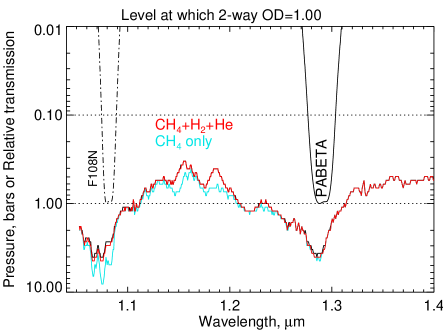
Figure 6.— Near-IR penetration depths vs. wavelength compared to filter transmission for F108N NICMOS and PaBeta Keck/NIRC2 filters, which sense similar atmospheric levels in a clear atmosphere, but are dominated by different gas absorptions (H₂ and CH₄ respectively).

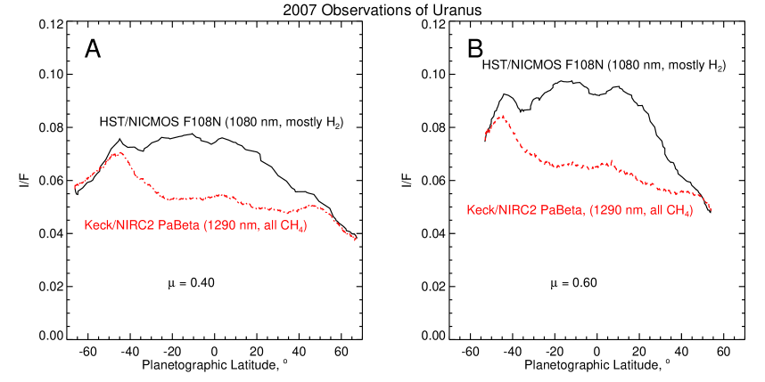
Figure 7.— Latitudinal profiles at fixed zenith angle cosines of 0.4 (A) and 0.6 (B) for F108N and PaBeta (Keck/NIRC2) filters taken near the Uranus equinox in 2007. At this point the southern hemisphere was still generally brighter than the northern hemisphere and the 38^∘ S - 58^∘ S southern bright band was still better defined and considerably brighter than the corresponding northern bright band. The relatively low equatorial I/F values for the methane-dominated PaBeta filter (1290 nm) indicates increased CH₄/H₂ absorption at low latitudes.

4.2. Direct comparison of key STIS wavelength scans

A similar spectral comparison of the 2012 STIS observations can also be informative. By selecting wavelengths that at one latitude provide similar I/F values but very different contributions by H₂ CIA and methane, one can then make comparisons at other latitudes to see how I/F values at the two wavelengths vary with latitude. If aerosols did not vary at all with latitude, then this would be a clear measure of the ratio of CH₄ to H₂. Fig. 8 displays a detailed view of I/F spectral region where hydrogen CIA exceeds methane absorption (see Fig. 2 for penetration depths). Near 930 nm and 827 nm the I/F values are similar but the former is dominated by methane absorption and the latter by hydrogen absorption. Near 835 nm there is a relative minimum in hydrogen absorption, while methane absorption is still strong. At 50^∘ N latitude and $\mu$=0.6, I/F values are nearly the same at all three wavelengths, suggesting that they all produce roughly the same attenuation of the vertically distributed aerosol scattering. At low latitudes, as shown in Fig. 9A, the I/F for the hydrogen-dominated wavelength increases, while the I/F for the methane-dominated wavelength decreases substantially, indicating an increase in the amount of methane relative to hydrogen at low latitudes. Similar effects are seen for the 2002 observations. For $\mu$=0.8 (Fig. 9B), which probes more deeply, the changes are even more dramatic. A color composite of these wavelengths (using R=930 nm, G= 834.6 nm, and B= 826.8 nm) is shown in Fig. 10, where the three components are balanced to produce comparable dynamic ranges for each wavelength. This results in nearly blue low latitudes where absorption at the two methane dominated wavelengths is relatively high and green/orange polar regions as a result of the decreased absorption by methane there.

Figure 8.— I/F and absorption spectra comparing the equilibrium H₂ CIA coefficient spectrum (divided by 1.2e-7, shown as dot-dash curve) and methane absorption coefficient spectrum (dashed). Note that the I/F spectrum has nearly equal I/F values at 826.8 nm (A), 834.6 nm (B), and 930 nm (C), but H₂ absorption is much greater at A than at B, while the opposite is true of methane absorption, and at C only methane absorption is present. In a reflecting layer model, changes in cloud reflectivity should affect wavelengths A-C by the same factor, but changes in methane mixing ratio would affect C most and A least.

Figure 9.— I/F vs latitude at $\mu=0.6$ (A) and $\mu=0.8$ (B) for three wavelengths with different amounts of methane and hydrogen absorption. Thin curves are from 2002 and thick curves from 2012. These are plots of center-to-limb fitted values instead of raw image data. In both cases the methane-dominated wavelengths have much reduced I/F at low latitudes. The 2002 calibration is based on WFPC2 comparisons and leads to I/F values 3% lower than the original KT2009 calibration.

The spectral comparisons in Figs. 9 and 10 also reveal substantial secular changes between 2002 and 2012. At wavelengths for which methane and/or hydrogen absorption are important, the northern low-latitudes have brightened substantially, while the southern low latitudes have darkened. The 2002-2012 differences shown in Fig. 9 are not due to a view-angle effect because comparisons in that figure are made at the same view and illumination angles for both years. The bright bands between 38^∘ and 58^∘ (north and south) have also changed significantly, with the southern band darkening dramatically, while the northern band brightened by a smaller amount. The northern bright band in 2012 was of lower contrast than the southern bright band in 2002. However, at continuum wavelengths (see Fig. 4 in the analysis supplement file) secular changes are not evident. Aside from what appears to be a small calibration disagreement between 2002 and 2012, in which corrected 2002 I/F values are about 2% higher (at continuum wavelengths), the latitudinal variations are very similar for both epochs. [The corrected 2002 calibration we use here is based on WFPC2 comparisons and leads to I/F values that are 3% smaller than published by KT2009.] The small size of these continuum differences is partly a result of the relatively smaller impact of particulates at short wavelengths where Rayleigh scattering is more significant. At absorbing wavelengths the optical depth and vertical distribution of particulates have a greater fractional effect on I/F and thus small secular changes in these parameters can be more easily noticed.

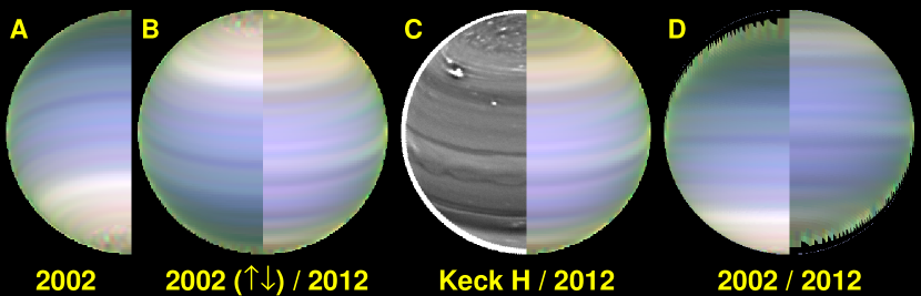
Figure 10.— Color composites of fitted center-to-limb smoothed images for 2002 (A, B, D) and 2012 (B-D) using color assignments R = 930 nm (all methane), G = 834.6 nm (methane and hydrogen), and B = 826.8 nm (mostly hydrogen). North is up in all images except the reflected 2002 image in B. The blue tint at low latitudes for both years is due to locally increased methane absorption. In B the 2002 image is inverted after remapping to the same central latitude as the 2012 image. The obvious asymmetry is not surprising because Uranus was in southern fall in 2002 and northern spring in 2012. In C we compare 2012 STIS observations with a Keck/NIRC2 near-IR image taken in the same year, high-pass filtered to enhance cloud structure. Note the small cloud features north of the high-latitude bright band. In D we compare 2002 and 2012 STIS observations at the same latitudes (i.e. without reflection of 2002 about the equator) and with both observations remapped to place the equator at the center of the image. In D the enhancement is the same for both 2002 and 2012, but using the 2012 albedo calibration function for both data sets (the solid curve in Fig. 4). The southern high latitudes in 2002 were brighter and whiter than corresponding northern latitudes in 2012, providing evidence for a seasonal lag. The dark band near the center of the two images is 5^∘ south of the equator. A comparison of latitudinal variations at fixed view angles is provided in Fig. 9.

5. A simplified model of methane/hydrogen variations

Here we model detailed relative latitudinal variations in effective methane mixing ratios using a simplified fast spectral model that we put on an absolute scale with selected full radiative transfer model results.

5.1. Model description

KT2009 estimated the latitude variation of the CH₄ volume mixing ratio using a simple model to fit the spectral region where hydrogen and methane have comparable effects on the observed I/F spectrum. They assumed that in the region from 819 nm to 835 nm the I/F spectrum could be approximated by

$$I/F=\exp(C_{0}+C_{1}\times k_{CH_{4}}+C_{2}\times k_{H_{2}}),$$ (2)

where $k_{CH_{4}}$ and $k_{H_{2}}$ are absorption coefficients of methane and hydrogen respectively. While this looks like a reflecting-layer model, it is actually more general. The coefficients $C_{1}$ and $C_{2}$ give the weighted path lengths of observed photons. Because the methane coefficient is essentially independent of temperature and pressure, the weighting for coefficient $C_{1}$ is the methane mixing ratio. But because $k_{H_{2}}$ not only depends on temperature, but also on the square of the density, $C_{2}$ has a pressure-dependent weighting. Mean path lengths are also affected by aerosols. The observed variation of $C_{2}$ is about 10 % peak-to-peak, aside from features that are consistent with noise. We expect that C₁ would have a similar variation if the methane mixing ratio is constant with latitude, and if the path lengths of photons do not vary much across the selected spectral region. Because $C_{1}$ and $C_{2}$ have different weightings, one might expect a little different variation for $C_{1}$, perhaps 5 % or 15 %. Thus, if the ratio $C_{1}/C_{2}$ shows latitudinal variations of about 5 %, that could be due to aerosols. If they are much larger, it strongly suggests that they are due to a variation of the methane mixing ratio. Whether the path lengths vary across the spectral region or not can be tested by fitting the spectral shape with Eq. 2. The fits shown in Fig. 11 are good. In fact, the slight misfit at the peak of the curves is likely due to a slight change of path lengths, indicating that the chosen spectral interval cannot be expanded without introducing systematic errors. To evaluate the hydrogen absorption coefficient, KT2009 used an effective fixed temperature of 80 K, which we also used because it provided an approximate overall best fit to the spectra over a range of latitudes. We also followed KT2009 in assuming equilibrium hydrogen.

Figure 11.— The 2012 I/F spectrum (solid curves) from 815 to 835 nm at $\mu$=0.6 for two sample latitudes: 0^∘ (left) and 65^∘ (right), using the simplified model (+) of Eq. 2, as discussed in the text. Also shown are relative variations of absorption by methane (dotted) and H₂ (dot-dash for para and double-dot-dash for ortho).

While KT2009 chose ten 1.6-nm wide segments from 819 to 835 nm, we here extended the range down to 815 nm to better sample the para hydrogen absorption peak near that wavelength, giving us 50 wavelengths over this range. The disadvantage of the wider interval is that fit quality is lower and somewhat more variable. However, sample calculations show very little difference in the derived latitudinal profile. In computing the $\chi^{2}$ estimates of fit quality, we assumed a somewhat arbitrary value of 2% in relative I/F calibration-absorption modeling error and combined that with the center-to-limb fitting errors using the root of the summed squares. We used an arbitrary scaling of the $k_{H_{2}}$ coefficients, then carried out a non-linear regression to obtain best fit model coefficients, uncertainties, and the ratio of $C_{1}/C_{2}$ and its uncertainty. Additional uncertainty is present due to the simplifications of the assumed model physics. The sample fits provided in Fig. 11 show that the model is quite successful at fitting the observed spectra, and also allows tight constraints on the model coefficients and on the ratio of coefficients, which we use as a proxy for the CH₄ /H₂ ratio. Section 5 of the on-line analysis supplemental file provides a more extended discussion of this model and our attempts to constrain both effective temperature and hydrogen para fraction as well as relative absorber amounts.

5.2. Model results for latitude dependence of CH₄/H₂.

Fitting this crude model to every latitude for both 2002 and 2012 center-to-limb fits leads to the latitude dependence shown in Fig. 12, where latitudes shown for each data set include the measured ranges and slight extrapolations of about 7^∘ of latitude (the modest uncertainties of such projections are illustrated in Fig. 2 of the on-line supplement). The estimated error bounds shown here, which are twice as large as the formal fitting errors, are based on splitting the spectral data into two independent subsets and comparing the two profile results. Here we use a scaling of the $C_{1}/C_{2}$ ratio that best matches the methane volume mixing ratio (VMR) values estimated from full radiation transfer modeling that properly accounts for the density dependence and temperature dependence of hydrogen absorption (discussed in subsequent sections). It is noteworthy that a single scale factor applied to all latitudes yields consistency with the full radiation transfer results at three different latitudes with different aerosol reflectivities. Using the same scale factor on the 2002 profile leads to about a 4% overall average between 30^∘ S and 20^∘ N. There are substantial differences between 2002 and 2012 where the two profiles overlap, though many of the small scale variations occur at nearly the same latitudes. The relative variations between 35^∘ S and 35^∘ N have a correlation of 70%, with the 2012 variations being about 10% larger than the 2002 variation. Yet the average 2012 methane VMR is closer to 4.5% at low southern latitudes where the 2002 profile is closer to 3.8%. Some of this difference might be due to the difference in aerosol structure, which is indicated by the higher reflectivity of the southern hemisphere in 2002 (see Fig. 9). Most of the small scale variability seen in the 2002 ratio is due to the hydrogen absorption term. Because this occurs without any evident small scale variability in the aerosol term (Fig. 9B), it suggests the possibility that small-scale temperature variations or vertical mixing variations that produce changes in para fractions might be responsible (this is discussed further in the next paragraph). A significant part of the small scale structure seen in the 2012 methane VMR values is also due to hydrogen coefficient variations, especially north of 60^∘ N where the model cloud reflectivity varies relatively smoothly with latitude (Fig. 12B), at least at these wavelengths (small variations are seen at near-IR wavelengths, as discussed later).

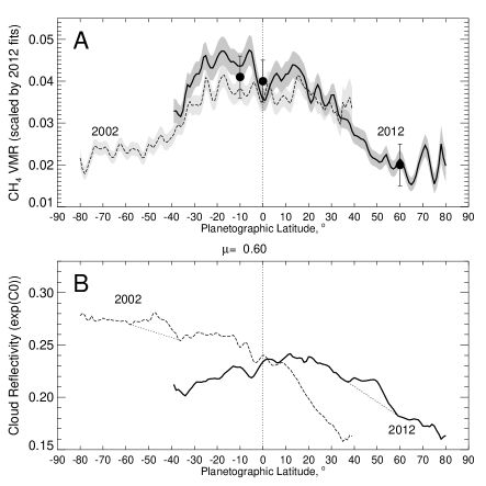
Figure 12.— A: Latitude dependence of the ratio $C_{1}/C_{2}$, which is crudely proportional to the CH₄/H₂ mixing ratio, scaled to best match the 2012 CH₄ VMR estimates at 10^∘ S, the equator, and 60^∘ N, obtained from radiation transfer modeling. Those results are plotted as larger filled circles with error bars. The same scaling used on the 2002 data (thin dashed line) leads to a slightly lower methane VMR at low latitudes. Error bars for the $C_{1}/C_{2}$ ratio points are provided only for scattered samples for clarity. B: The aerosol reflectivity term (exp(C0)), for 2002 and 2012, using the KT2009 spectral calibration divided by 1.03 for 2002 results. Dotted lines interpolate across the regions where bright bands are seen (38^∘ - 58^∘).

Also noteworthy is the difference between 2012 north and 2002 south polar regions (there is no overlap between 2002 and 2012 in either polar region). In 2002 the mixing ratio from 75^∘ S to 50^∘ S is close to 2.4% and exhibits only small variations with latitude, while the 2012 profile at equivalent northern latitudes displays substantial and nearly sinusoidal variations with a latitudinal wavelength near 10^∘. It should be noted that each of these points is derived from 50 wavelengths and is thus far less noisy than one might suspect based on the plots of single wavelengths, as in Figs. 9 and 10. The reality of these high-latitude features is further supported by the fact that the same analysis applied to similar latitudes in the opposite hemisphere using 2002 observations did not find such large variations, suggesting that the variations are more likely due to a hemispheric difference rather than an inherent high latitude artifact of the analysis. Also, there is no obvious reason why such artifacts should suddenly disappear at latitudes below 60^∘ N. Further evidence supporting the reality of these latitudinal variations in the methane to hydrogen absorption ratio is the discovery of a correlated pattern of cloud reflectivity variations in high-resolution Keck imagery, which is discussed in the analysis supplement file. A hint of this pattern can also be seen in Fig. 10C. We found similar patterns in August and November images and both had moderately significant negative correlations with the methane VMR ($\sim$ 9 % for August and($\sim$ 5-10 % for November). While the correlations are suggestive, it is still possible that the STIS latitudinal variation is due to noise and new observations will be needed to confirm this feature. The explanation for this feature, presuming that it is real, might be that latitude bands of reduced above-cloud methane lead to clouds appearing locally brighter due to reduced methane absorption. An alternate explanation is that the local variation in methane to hydrogen absorption is due to changes in the para fraction of hydrogen. If we force the methane mixing ratio to be constant over the 55^∘ - 82^∘ latitude range and fit spectral variations by adjusting the para fraction and effective temperature, then para fraction increases appear where we previously had methane decreases. The para increases suggest downwelling and thus we have a correlation of descending motion with reduced cloud amount (or reduced cloud reflectivity). This alternative interpretation presents a more appealing picture than our initial interpretation, although it has a slightly worse spectral fit quality.

6. Full radiative transfer modeling of methane and aerosol distributions

The spectral profile comparisons (Figs. 7, 8, and 9), and especially the somewhat more quantitative modeling of Fig. 12, strongly suggest that there is a permanent and more or less symmetric high latitude methane depletion on Uranus. But, because hydrogen absorption has a density squared dependence, and the methane has a vertically varying mixing ratio, a more accurate constraint on methane requires full radiative transfer modeling, including the effects of more realistic aerosol distributions, as described in the following. The more complete modeling is also needed to provide the scaling factor that converts the $C_{1}/C_{2}$ ratio plotted in Fig. 12 to a methane VMR.

6.1. Radiation transfer calculations

We used the radiation transfer code described by Sromovsky (2005a), which include Raman scattering and polarization effects on outgoing intensity, though this is a minor virtue at the wavelengths employed in our analysis. To save computational time we employed the accurate polarization correction described by Sromovsky (2005b). After trial calculations to determine the effect of different quadrature schemes on the computed spectra, we selected 14 zenith angle quadrature points per hemisphere and 14 azimuth angles. Calculations with 10 quadrature points and 10 azimuth angles changed fit parameters by only about 1%, which is much less than their uncertainties. To characterize methane absorption at CCD wavelengths we used the coefficients of KT2009. To model collision-induced opacity of H₂-H₂ and He-H₂ interactions, we interpolated tables of absorption coefficients as a function of pressure and temperature that were computed with a program provided by Alexandra Borysow (Borysow et al. 2000), and available at the Atmospheres Node of NASA’S Planetary Data System. We assumed equilibrium hydrogen for most calculations, following KT2009 and Sromovsky et al. (2011).

6.2. Cloud model

The cloud model we used (referred to as the compact model in what follows) is a modification of the KT2009 diffuse model (containing 4 vertically extended layers) that is fully described in Section 7 of the supplemental analysis file. Our five-layer model is illustrated in Fig. 13 and summarized in Table 2. In this table, parameter names begin with $m$ for layers containing Mie particles and with $hg$ for layers containing particles with double Henyey-Greenstein phase functions. Here we use Mie particle scattering as a convenient parameterization of wavelength dependence, realizing that the particles are generally not spherical. Adjustable parameters are identified in the Value column of the table. We chose this model because it provided substantially better fits than the diffuse model. Our top two haze layers use the same parameterization as KT2009. The main change we made to the KT2009 model was to replace its middle tropospheric layer with two compact layers: an upper middle tropospheric cloud layer (UMTC) and a lower middle tropospheric cloud layer (LMTC). The UMTC layer is composed of Mie particles, which we characterized by a gamma size distribution with an adjustable mean particle radius and a fixed normalized variance of 0.1, a fixed refractive index of 1.4, and an imaginary index of zero. For the LMTC layer we used particles with the same scattering properties as given by KT2009 for their tropospheric particles. Both of these compact layers have the bottom pressure as a free (adjustable) parameter and a top pressure that is a fixed fraction of 0.93 $\times$ the bottom pressure. This degree of confinement is approximately the same as obtained for the cloud layer inferred from the radio occultation analysis (Sromovsky et al. 2011). The motivation for introducing these replacement layers was to obtain more flexibility in vertical structure and to allow the possibility of including a thin cloud near the methane condensation level, as suggested by the occultation analysis.

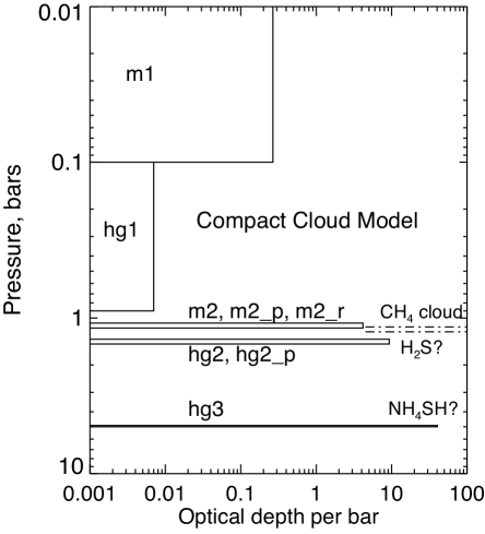
Figure 13.— Compact cloud model vertical structure. Compared to the KT2009 model, this has two layers with additional adjustable parameters of base pressure (for the new $hg2$ layer) and base pressure and particle radius (for the new $m2$ layer).

Table 2Compact cloud model parameters

	Parameter/function	Value
Stratospheric haze	$m1\_pd$ (bottom pressure)	fixed at 100 mb
of Mie particles	$m1\_r$ (particle radius)	fixed at 0.1 $\mu$m
with gamma size	$m1\_b$ (variance)	fixed at 0.3
distribution	$n1$ (refractive index)	nr=1.4, ni given by KT2009
	$m1\_odpb$ (optical depth/bar)	adjustable1
Upper tropospheric haze	$hg1\_pd$ (bottom pressure)	fixed at 0.9 bars (top pressure = $m1\_pd$)
of double HG particles	$\varpi(\lambda)$ (single-scatt. albedo)	KT2009 function
(UTH)	phase function (KT2009)	$g_{1}=0.7$, $g_{2}=0.3$, $f_{1}(\lambda)$ given by KT2009
	$hg1\_odpb$ (optical depth/bar)	adjustable2
Upper middle tropospheric	$m2\_p$ (bottom pressure)	adjustable3 (top pressure = $m2\_p\times$0.93)
cloud layer of Mie	$m2\_r$ (particle radius)	adjustable4
particles (UMTC)	$m2\_b$ (variance)	fixed at 0.3
	$n2$ (refractive index)	fixed at n=1.4
	$m2\_od$ (optical depth)	adjustable5
Lower middle tropospheric	$hg2\_p$ (bottom pressure)	adjustable6 (Ptop = $hg2\_p$ X 0.9)
cloud of double HG	$\varpi(\lambda)$ (single-scatt. albedo)	given by KT2009
particles (LMTC)	phase function (KT2009)	$g_{1}=0.7$, $g_{2}=0.3$, $f_{1}(\lambda)$ given by KT2009
	$hg2\_od$ (optical depth)	adjustable7
Bottom tropospheric cloud	$\varpi(\lambda)$	same as previous layer
(BTC)	phase function (DHG)	same as previous layer
	$hg3\_od$ (optical depth)	adjustable8
	$hg3\_p$ (bottom pressure)	fixed at 5 bars

NOTE: KT2009 equations defining wavelength dependent parameters are reproduced in the analysis supplement file. Usually $hg1\_odpb$ was found to be too small to bother including in our fits.

The last change we made was to replace the KT2009 bottom tropospheric layer by a compact cloud layer at 5 bars (the BTC, or bottom tropospheric cloud), with adjustable optical depth and with the KT2009 tropospheric scattering properties. Sromovsky et al. (2011) found that this layer was needed to provide accurate fits near 0.56 and 0.59 $\mu$m, but its pressure was not well constrained by the observations (pressure changes could be compensated by optical depth changes, to produce essentially the same fit quality). Whether this deep cloud is vertically diffuse or compact also could not be well constrained. Sample phase functions and the scattering properties of particles used in our cloud model are plotted vs. wavelength in the analysis supplement file (Section 7). Note that the KT2009 empirical functions defining wavelength-dependent single-scattering albedo and phase functions only apply over the 300 nm to 1000 nm range for which they were derived. The role played by each model layer in creating a spectrum that matches sample observations is also provided in the analysis supplement file (Section 8).

6.3. Fitting procedures

To avoid the complexity of fitting a wavelength-dependent imaginary index in the methane layer (the UMTC layer in Table 2) we fit only the wavelength range from 0.55 $\mu$m to 1.0 $\mu$m. We chose a wavenumber step of 118.86 cm^-1 for sampling the observed and calculated spectrum. This yielded 69 spectral samples, each at three different zenith angle cosines (0.3, 0.4, and 0.6), for a total of 207 points of comparison. Our compact layer model has seven to eight adjustable parameters (see Table 2), leaving 201 or 200 degrees of freedom ($N_{F}$) respectively. (The expected value of $\chi^{2}$ is equal to $N_{F}$ for an optimized fit, and the formal uncertainty in any fit parameter is given by the change in its value that increases $\chi^{2}$ by one unit when the remaining parameters are optimized (Press et al. 1992).) We fixed the BTC base pressure to 5 bars (see Table 2) and usually ignored the UTH layer because of its negligible effects. We used a modified Levenberg-Marquardt non-linear fitting algorithm (Sromovsky and Fry 2010) to adjust the fitted parameters to minimize $\chi^{2}$ and to estimate uncertainties in the fitted parameters. Evaluation of $\chi^{2}$ requires an estimate of the expected difference between a model and the observations due to the uncertainties in both. We followed the same approach for estimating uncertainties as used by Sromovsky et al. (2011), which combined measurement noise (estimated from comparison of individual measurements with smoothed values), modeling errors of 1%, relative calibration errors of 1% (larger absolute calibration errors were treated as scale factors), and effects of methane absorption coefficient errors, taken to be random with RMS value of 2% plus an offset uncertainty of 5$\times 10^{-4}$ (km-amagat)^-1. The uncertainty in $\chi^{2}$ is expected to be $\sim$25, and thus fit differences within this range are not of significantly different quality.

7. Compact model fits

The compact model described previously provides generally better fits than the diffuse models, reaching $\chi^{2}$ values in the low to mid 200’s compared to mid 300’s to low 500’s for the diffuse model. This is presumably due to its greater flexibility to fit vertical distributions because the main cloud layer is divided into two sublayers with adjustable pressures as well as adjustable optical depths. Another difference from diffuse models is that its upper sublayer has its wavelength dependence controlled by Mie scattering, which is parameterized by particle radius and refractive index, rather than the wavelength-dependent double Henyey-Greenstein parameters of of the lower sublayer, which we take to be those of KT2009 and reproduced in the analysis supplement file.

In the following, we first constrain the effective methane mixing ratio profile at key latitudes to define the scaling factor for Fig. 12, then try to fit cloud structure to the observed spectra over a wide range of latitudes, using the best-fit equatorial methane vertical profile to discover where it does not apply. Poleward of 30^∘ N we obtain improved fits by reducing the effective mixing ratio. But the best fits are obtained with a depletion profile that exhibits decreasing depletion with increasing depth, which also is more physically plausible than a uniform depletion at all depths. In other words, the preferred latitudinal profile of methane becomes more uniform at greater depths.

7.1. Constraining equivalent methane mixing ratios at key latitudes

The detailed latitudinal variation of the equivalent methane mixing ratios plotted in Fig. 12 is based on a scaled ratio of fit coefficients ($C_{1}/C_{2}$). To define that scaling, we used fits that fully account for the different vertical absorption profiles of hydrogen CIA and methane, carried out at three latitudes covering the range of mixing ratio variation (10^∘ S, 0^∘, and 60^∘ N). To estimate the optimum equivalent deep methane mixing ratio at each latitude we did compact model fits for a variety of methane profiles (D1, DE, E1, EF, F1, FG, and G) that have a range of deep methane mixing ratios (2.22%, 2.76%, 3.20%, 3.6%, 4.00%, 4.5%, and 4.88%, respectively). These profiles are all consistent with the Voyager 2 occultation measurements of Lindal et al. (1987), and thus also have different temperature and above-cloud methane profiles. They are all from Sromovsky et al. (2011) except for DE and FG, which we constructed to be occultation consistent using the same techniques as Sromovsky et al. (2011). The fit results at our selected key latitudes are plotted in Fig. 14, where we show two fit quality measures as a function of the deep methane mixing ratio of the profiles that were employed. The two measures are (1) $\chi^{2}$ and (2) the signed error at 825 nm divided by the error expected just from measurement errors. At 10^∘ S the minimum $\chi^{2}$ occurs at a lower methane mixing ratio (3.6%) than the minimum error at 825 nm (4.6%), while at the equator the two measures agree on 4%. For 60^∘ N, we find by extrapolating that the 825-nm error reaches zero at 1.6%, while the corresponding $\chi^{2}$ minimum is between 2.2% and 2.6%. We consider the 825-nm estimate to be the most relevant since it provides the most direct comparison between methane and hydrogen absorptions and uses the $\mu$ = 0.6 spectrum to weight the deep atmosphere more than the overall fit, which uses $\mu$ = 0.3, 0.4, and 0.6. However, its greater uncertainty limits led us to use intermediate estimates between these two measures: 4.1$\pm$0.5% at 10^∘ S, 4.0$\pm$0.5% at the equator, and 2.0$\pm$0.5% at 60^∘ N. These points were plotted in Fig. 12 as filled circles. That these results lead to such a consistent scaling for the simplified model justifies its use in estimating latitudinal variations. The low-latitude average mixing ratio is sufficiently close to the F1 profile value of 4% that we used F1 as our base profile.

Note that an occultation consistent profile with a deep mixing ratio as low as 1.6%, which is the deep VMR assumed by Tice et al. (2013), would be grossly inconsistent with the observed spectra at low latitudes. Though Tice et al. (2013) were able to fit their spectra with such low methane VMR values, they may have been able to make up for lacking methane absorption at longer wavelengths by assuming a low single-scattering albedo in their main cloud layer. Also, based on sample spectral fits shown in their Figs. 4, 7, and 15, they did not fit very well the critical spectral region near 825 nm, where their model spectra show relatively more hydrogen absorption than the observations, which suggests that their methane mixing ratio is too low. They also reduce the weight of this spectral region in their fits by assigning relatively large uncertainties compared to other regions with similar I/F values. Their fits were also aided by using much more above-cloud methane than would be allowed by the 0% relative humidity implied by the Voyager 2 occultation results of Lindal et al. (1987) for their assumed deep mixing ratio.

Figure 14.— Best-fit compact model parameters vs deep methane mixing ratio for undepleted occultation-consistent D1, E1, EF, F1, and G profiles from Sromovsky et al. (2011), and DE and FG profiles created using the same procedure. The fits are to STIS spectra at 10^∘ S, the equator, and 60^∘ N, for zenith angle cosines of 0.3, 0.4, and 0.6. The $\chi^{2}$ values are shown with solid curves, and the 825-nm error ratio to expected error at $\mu$=0.6 is shown with dotted curves. Horizontal arrows indicate which axis to read in each case.

7.2. Compact model fits versus latitude for the F1 profile

We first tried to fit the compact model to a range of latitudes, while assuming that the F1 profile of temperature and methane applied to all latitudes. The entire set of results is plotted in Fig. 15, and results for latitudes up to 30^∘ N are presented in Table 3. There are several remarkable features of these fits. First, the $m1$ vertically diffuse stratospheric haze layer is found to have significantly reduced opacity north of 25^∘ N. Whether this is a real effect and a real change from the structure inferred from 2002 observations or a result of a different spectral calibration using WFC3 observations is unknown. Perhaps a related difference is that the upper sublayer (UMTC) of the main cloud layer, a Mie layer, has a fitted particle radius generally in the 0.2-0.5 micron range, compared to the 1.2-micron radius that seemed to be preferred by the Sromovsky et al. (2011) analysis of 2002 STIS observations. This is likely due to the revised albedo calibration function (Fig. 4), which produces a stronger I/F decline with wavelength that is better matched by smaller particles (see analysis supplement file).

Table 3Best-fit parameters for equatorial compact cloud layer models versus latitude assuming simulated F1 profile for latitudes between 30^∘ S and 30^∘ N, and using depleted F1 profiles for higher latitudes.

Lat.	$m2\_p$	$hg2\_p$	$m1\_odpb$	$m2\_od$	$hg2\_od$	$hg3\_od$	$m2\_r$	$\chi^{2}$	(m-o)/u
∘	bar	bar					$\mu$m
-30	1.19$\pm$0.03	1.41$\pm$0.02	0.21$\pm$0.04	0.34$\pm$0.09	0.96$\pm$0.05	4.09$\pm$0.75	0.32$\pm$0.12	299	-0.32
-20	1.31$\pm$0.03	1.51$\pm$0.04	0.25$\pm$0.04	0.46$\pm$0.11	0.94$\pm$0.07	3.64$\pm$0.90	0.19$\pm$0.01	373	0.69
-10	1.25$\pm$0.02	1.52$\pm$0.03	0.42$\pm$0.04	0.39$\pm$0.09	1.10$\pm$0.07	3.84$\pm$0.90	0.18$\pm$0.03	338	0.85
0	1.18$\pm$0.02	1.48$\pm$0.03	0.62$\pm$0.03	0.43$\pm$0.07	1.19$\pm$0.06	3.94$\pm$0.67	0.47$\pm$0.05	205	-0.07
10	1.27$\pm$0.02	1.47$\pm$0.03	0.34$\pm$0.04	0.47$\pm$0.10	1.12$\pm$0.07	4.83$\pm$1.09	0.16$\pm$0.02	359	1.00
20	1.26$\pm$0.02	1.47$\pm$0.03	0.26$\pm$0.04	0.48$\pm$0.10	1.16$\pm$0.07	5.42$\pm$1.20	0.19$\pm$0.03	344	0.29
30	1.19$\pm$0.02	1.36$\pm$0.02	0.09$\pm$0.04	0.24$\pm$0.04	1.01$\pm$0.04	5.05$\pm$0.72	0.20$\pm$0.02	227	0.52
38	1.24$\pm$0.03	1.58$\pm$0.03	0.23$\pm$0.03	0.37$\pm$0.07	0.95$\pm$0.05	2.84$\pm$0.44	0.47$\pm$0.06	204	-0.23
45	1.23$\pm$0.04	1.53$\pm$0.03	0.21$\pm$0.04	0.38$\pm$0.09	1.06$\pm$0.06	1.86$\pm$0.43	0.45$\pm$0.08	307	-0.18
50	1.17$\pm$0.05	1.57$\pm$0.02	0.09$\pm$0.05	0.27$\pm$0.04	1.07$\pm$0.04	1.07$\pm$0.24	0.22$\pm$0.02	226	0.29
60	1.24$\pm$0.05	1.70$\pm$0.04	0.12$\pm$0.04	0.36$\pm$0.06	0.82$\pm$0.03	0	0.43$\pm$0.05	234	0.14
70	1.32$\pm$0.05	1.85$\pm$0.07	0.04$\pm$0.04	0.48$\pm$0.08	0.65$\pm$0.04	0	0.43$\pm$0.05	246	0.33

Note: The fits from -30^∘ to 30^∘ were done using the F1 thermal and methane profile, which has a deep methane volume mixing ratio of 4%, and a He/H₂ ratio of 0.1306. At other latitudes the fits used methane depleted profiles with $vx$=3.0 and depletion depths between the value that minimizes 825-nm errors and those that minimize $\chi^{2}$ (both listed in Table 4 and plotted in Fig. 15). The uncertainty in $\chi^{2}$ is $\sim$25 and thus fits differing by less than this are not of significantly different quality. The column labeled $(m-o)/u$ is the fit error at 0.825 $\mu$m expressed as the ratio of (model I/F - observed I/F) to the estimated I/F uncertainty for $\mu$ = 0.6. These results are plotted in Fig. 15. The parameter $hg1\_odpb$ was omitted from these fits for reasons discussed in the main text.

At the equator the results are also unusual. In diffuse model fits we found that the upper tropospheric haze (the second layer in Table 2) provided a sharply increased contribution at the equator, and seemed to be the main change associated with the bright equatorial band visible in many images at wavelengths of intermediate methane absorption (e.g. Fig. 3K, and S). In the compact model fits, however, changes in the next lower and higher layers (first and third layers in Table 2) seem to be relatively more important, with changes in pressure and particle size of the third layer ($m2\_p$ and $m2\_r$) as well as the optical depth per bar of the top layer ($m1\_odpb$) playing a role. The derived value of the optical depth per bar of the second layer ($hg1\_odpb$) for the compact model is comparable to its uncertainty and was ignored for most compact model fits.

Between 30^∘ S and 30^∘ N, the 825-nm signed error, given by (model-observed)/uncertainty, is relatively flat. The small positive error seen in this at most latitudes in this range suggests that the mixing ratio in the F1 profile is not quite large enough. The rather large negative 825-nm errors found at high latitudes are associated with excessively high methane mixing ratios in the model calculations. The $\chi^{2}$ measure of fit quality is generally low, but is a more erratic function of latitude over this range. Beyond 40^∘ N, the 825-nm signed error becomes much larger as the overall fit quality measured by $\chi^{2}$ becomes much worse. This indicates that the assumed latitude-independent profile of methane is not consistent with the observations. A different methane profile is clearly needed at high latitudes as was already demonstrated at 60^∘ N from fits used to define the scaling of the simplified model.

Figure 15.— Best-fit compact model parameters vs. latitude assuming the F1 structure and methane mixing ratio profile (left) and using the best-fit depletion depth profiles (right). Error bars indicate fitting uncertainty. In each case, the lower panel displays fit quality in terms of $\chi^{2}$ (+) and signed 825-nm error (o). In the bottom left plot, the behavior of the 825-nm error indicates that the actual methane absorption declines below the assumed value beginning about 40^∘ N. In the bottom right plot, both 825-nm error and $\chi^{2}$ benefit from use of depleted profiles. In the bottom panels horizontal arrows indicate which axis to read for each curve.

7.3. Why methane depletion should not extend to great depths

While structure and methane profiles with a 2% CH₄ deep mixing ratio provide the best fits at 60^∘ N compared to other profiles with constant mixing ratios up to the condensation level, the deep contrast between equator and pole (2% VMR to 4% VMR) is not physically plausible. Such deep latitudinal gradients in composition would lead to density gradients along isobars. As a consequence of geostrophic and hydrostatic balance, these gradients would lead to vertical wind shears (Sun et al. 1991). These vertical wind shears acting over the entire atmosphere would likely lead to cloud top winds that would be highly incompatible with the observed winds. Thus we considered methane vertical distributions in which the higher latitudes had depressed mixing ratios restricted to shallow depths in the upper troposphere only. As indicated by KT2009, the 2002 spectral observations did not require that methane depletions extend to great depths, and Sromovsky et al. (2011) showed that shallow depletions were preferred by the 2002 spectra. We will show here that the 2012 spectral constraints favor relatively shallow methane depletions at middle latitudes but increasingly deeper depletions at high latitudes.

Here we constructed profiles with shallow CH₄ depletion using the “proportionally descended gas” profiles of (Sromovsky et al. 2011) in which the model F1 mixing ratio profile $\alpha(P)$ is dropped down to increased pressure levels $P^{\prime}(\alpha)$ using the equation

$$P^{\prime}=P\times[1+(\alpha(P)/\alpha_{d})^{vx}(P_{d}/P_{c}-1)],$$ (3)

for $P_{tr}<P<P_{d}$, where $P_{d}$ is the pressure depth at which the revised mixing ratio $\alpha^{\prime}(P)=\alpha(P^{\prime})$ equals the uniform deep mixing ratio $\alpha_{d}$, $P_{c}$ is the methane condensation pressure before methane depletion, $P_{tr}$ is the tropopause pressure (100 mb), and the exponent $vx$ controls the shape of the profile between 100 mb and $P_{d}$. The profiles with $vx=1$ are similar in form to those adopted by Karkoschka and Tomasko (2011).

7.4. Compact model fits at 60^∘ N vs depletion depth

To account for the lower methane mixing ratio that is observed at high latitudes we need to find a methane sink that can create local depletions. The most obvious one is methane condensation, which can cause the low-temperature above-cloud region to have much lower methane mixing ratios than the regions below. When this depleted gas is mixed downward, it can cause local depressions of the methane mixing ratio in the upper troposphere. Thus we expect only the upper troposphere to be depleted and a significant question is whether we can constrain the depth of that depression using STIS observations.

Here we start with an F1 profile at 60^∘ N and then use Eqn. 3 to deplete the methane above a base pressure $P_{d}$ at a rate controlled by a secondary parameter $vx$, which causes rapid depletion with decreasing pressure when set to small values and smaller depletion rates when set to larger values. Sromovsky et al. (2011) found that $vx=1$ seemed to be preferred by the 2002 data set, but we found larger values preferred by the 2012 data set (this might also be true for 2002 if explored more extensively and with the 2012 calibration function). We tried a range of $P_{d}$ values for $vx$ ranging from 1 to 5. Subsets of our results are plotted in Fig. 16, which displays $\chi^{2}$ and 825-nm error values as a function of $P_{d}$ for different assumed values of $vx$. The optimum values are summarized in Table 4. We found that $\chi^{2}$ minima appear at increasing depths as the depletions become more gradual with decreasing pressure (for larger values of $vx$). The best fit at 60^∘ N was found for $vx=3.0$, with $P_{d}=30$ bars to minimize $\chi^{2}$ and 16 bars to minimize the 825-nm error. For $vx=2$, the $\chi^{2}$ minimum is near 10 bars and somewhat larger than the minimum for $vx=3$, while the minimum 825-nm error is found at 7.5 bars, closer to the $\chi^{2}$ minimum than for the $vx=3$ case. Clearly, $vx=1$ is a very poor choice. But even that profile fits better ($\chi^{2}$ = 320) than the D1 profile ($\chi^{2}$ = 360), which is the best fitting of the occultation consistent profiles with vertically uniform mixing ratios. The vertical variation of methane VMR for the best fit $P_{d}$ value is shown for each $vx$ case in Fig. 17A. Note that shallower and deeper depletions all produce similar mixing ratios near 1.7 bars, and that greater depletions at depth result in somewhat higher mixing ratios at pressures below 1.7 bars. It should also be noted that the STIS measurements aren’t sensitive to the large depths implied by the best-fit $P_{d}$ values. It is fitting the shape of the empirical profile at much lower pressures that constrains the $P_{d}$ value. Thus it would be worthwhile to explore other depletion functions with different vertical variations.

Figure 16.— Fit quality estimates for compact cloud layer model fits to spectra at 60^∘ N ($\chi^{2}$ on left axis, 825-nm error on right), shown as function of depletion depth $p_{d}$ for depletion profiles with different $vx$ values. Depletions are relative to an F1 base model.

7.5. Latitudinal variation in depletion depth and aerosol structure

To fix the problem of poor spectral fits at latitudes beyond 30^∘ N, we chose $vx=2$ and $vx=3$ vertical variation functions and found the best-fit value of $P_{d}$ as a function of latitude for each. At all latitudes we found that $vx=3$ provided the best fits. The $\chi^{2}$ and 825-nm error results as a function of $P_{d}$ for $vx=3$ are plotted in Fig. 12 of the analysis supplement. Here we list best-fit $P_{d}$ values in Table 4 and the best-fit aerosol parameters in Table 3, where the aerosol model is chosen for $P_{d}$ values between those giving the smallest $\chi^{2}$ and those giving the smallest 825-nm error. The best-fit aerosol results are also plotted in Fig. 15 (right panels) for comparison with the fits using the undepleted F1 profile at all latitudes. The depletion depth increases from 30^∘ N to 70^∘ N (the highest latitude fit) and in this region $\chi^{2}$ and 825-nm errors have been greatly reduced relative to the prior fits with undepleted profiles.

Figure 17.— Depletion models for 60^∘ N with different $vx$ values (A) and best fit depletion models for different latitudes (B), assuming $vx$=3.0 for all latitudes.

One puzzling result is that the cloud layer that we thought was associated with methane condensation (the UMTC or $m2$ layer in Fig. 13) continues into the polar regions where methane condensation should not occur because of the decreased methane mixing ratio. Perhaps we should not have used the same labels for $m2$ points at high latitudes that we used at latitudes from 30^∘ S to 30^∘ N (see right panel of Fig. 15). In fact, the sharp drop in optical depth of the $m2$ layer between 20^∘ N and 30^∘ N might have continued northward, and what we identified as the $m2$ layer north of 30^∘, might actually be a continuation of the $hg2$ cloud. In that case, the layer we identified as the $hg2$ cloud in these northern fits might actually have a different composition from the corresponding layer at low latitudes. Also note that the $hg3$ layer declines dramatically north of 50^∘ N, where $Pd$ exceeds the assumed depth of the cloud layer. The polar region possibly has a completely new set of cloud layers.

Table 4Optimum depletion depth based on fit quality and 825-nm error as a function of depletion profile rate (small $vx$ provides sharper depletions above the depletion depth limit $p_{d}$).

Planetographic		minimum $\chi^{2}$			minimum 825-nm error
Latitude, ∘ N	$vx$	$p_{d}$	$\chi^{2}$	825-nm error	$p_{d}$, bars	825-nm error	$\chi^{2}$
38	2.0	2.0	215	-0.50	3.0	0.28	226
38	3.0	3.0	204	-0.23	4.0	0.10	207
45	2.0	2.0	318	-0.77	3.0	-.07	326
45	3.0	4.0	307	-0.18	4.0	-0.18	307
50	2.0	4	239	-0.01	4	-0.01	239
50	3.0	10	225	0.57	8	0.29	226
60	1.5	5.5	282	0.19	5.0	0.00	282
60	2.0	10	238	0.48	7.0	-0.12	252
60	3.0	30	227	0.60	16	0.01	242
60	5.0	200	243	0.34	90	-0.02	249
70	2.0	12	253	0.50	8	-0.18	263
70	3.0	30	246	0.33	20	-0.09	254

8. Discussion: Methane as a constraint on meridional motions.

Fig. 18 illustrates a mechanism for depleting methane at high latitudes that is essentially the same as what was previously suggested by KT2009. Rising methane-rich gas at low latitudes is dried out by condensation and sedimentation of methane ice particles. That dried gas is then transported to high latitudes, where it begins to descend, bringing down methane depleted gas, which then gets mixed with methane-rich gas on its return flow. The figure illustrates two different styles of return flow. Without lateral eddy mixing across the streamlines, the only restoration of the methane mixing ratio would be through evaporation of the precipitating condensed methane at low latitudes. The depth of the depletion at high latitudes might be controlled by the depth of the meridional cell or the depth at which cross-streamline mixing predominates. The suggested circulation would promote formation of optically thin methane clouds (or hazes) at low latitudes, but inhibit methane cloud formation at high latitudes. This seems consistent with the lack of observed discrete cloud features south of 45^∘ S. However, we have seen discrete cloud features at high northern latitudes (Sromovsky et al. 2009), which might very well be composed of something other than methane, given that their cloud tops seem to be deeper than the methane condensation level (Sromovsky et al. 2012). The general downwelling would also tend to inhibit all condensation clouds, as sub-condensation mixing ratios would be created by such motions. However, this does not rule out localized regions of upwelling and formation of condensation clouds occupying a small fractional area.

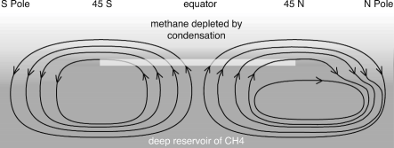
Figure 18.— Speculative meridional flows in which rising flows at low latitudes produce methane condensation (white region) that depletes the gas of methane; the depleted gas is transported to high latitudes where it descends to reduce the mixing ratio at higher pressure. The depletion depth might be limited by the depth of the circulation, or by lateral mixing. A very deep cell of this type has been inferred from microwave observations (see main text). Note that the streamlines of the northern cell provide an example of shallower depletions at intermediate high latitudes than those of the southern cell, the former option being more consistent with the observed increasing methane depletion depth at higher latitudes.

The circulation cell in Fig. 18 would need to be very deep to be consistent with microwave observations probing the 10-100 bar region of Uranus (de Pater et al. 1989, 1991; Hofstadter et al. 2007). These reveal a symmetry pattern in which microwave absorbers (NH₃, H₂S) are depleted at both high southern and high northern latitudes, suggesting a non-seasonal equator-to-pole meridional circulation, with upwelling at low latitudes and down-welling at high latitudes (de Pater and Lissauer 2010; de Pater et al. 1989, 1991; Hofstadter et al. 2007), similar to the circulation cells illustrated in Fig. 18. If this deep cell extended to the upper troposphere, it could be consistent with a shallow CH₄ depletion, as long as the flow at the several bar level was dominated by poleward flow that did not go through the drying-by-condensation process, as suggested by the inner streamline in the northern flow pattern in Fig. 18. While our best fits indicate that the largest fractional depletions occur in the upper troposphere, at higher latitudes some degree of depletion could extend deeper than the 10-bar level. Because these deep meridional cells would likely be dominated by deep atmospheric conditions, they would probably have the same symmetry properties as the deep atmosphere (symmetry about the equator), which would suggest qualitatively that the north and south polar regions should not look very different. With respect to the gross character of the methane depletion, they don’t look very different, even though they do exhibit different cloud morphologies.

A problem with a single deep cell in each hemisphere is that it would seem to inhibit formation of H₂S condensation clouds that are good candidates for producing the bright bands that form between 38^∘ and 58^∘ in both hemispheres. In fact, such a simple circulation would tend to inhibit all condensation clouds at high latitudes, in spite of the fact that cloud particles of some kind are detected there. A 3-layer circulation cell (Fig. 19) can provide more opportunities for condensation cloud formation. In this case the deep cell produces ammonia depletion through formation of an NH₄SH cloud at low latitudes, an intermediate cell produces high latitude condensation of H₂S, and the top cell provides high-latitude depletion of methane. This structure is also qualitatively compatible with the observed equatorward motion of the long-lived and largest discrete cloud feature seen on Uranus, known as the Berg (Sromovsky and Fry 2005; Sromovsky et al. 2009; de Pater et al. 2011). This feature is thought to have been at the level of the putative H₂S cloud, and in this model would ride along with the equatorial flow near the 1.5 bar level. However, the resemblance between the speculated structure in Fig. 19 and the structure shown in the right panels of Fig. 15 is crude at best. While there seems to be a change in cloud structure between high and low latitudes, if the interpretation is restricted to models with condensation clouds only, it is hard to explain the existence of what seems to be an H₂S cloud at low latitudes where the three-layer cell structure would inhibit such a cloud. Furthermore, the drift of the Berg may not be a relevant constraint on meridional flow. If the cloud features comprising the Berg were generated by an unseen vortex, its drift may be controlled more by the vorticity of the zonal flow than by weak meridional flows (Lebeau and Dowling 1998).

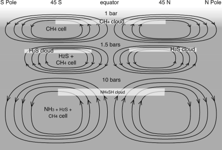
Figure 19.— Speculated 3-layer cell structure providing equatorward flow at the berg level and poleward flow above methane condensation and NH₄SH cloud formation levels. Here cloud formation/condensation regions are indicated by light rectangles.

An additional problem with the above suggested meridional circulation structures is that they do not appear to be consistent with Voyager observations. Using thermal emission measurements by the Voyager IRIS instrument in 1986 Flasar et al. (1987) inferred upwelling motions at $\pm$30^∘, where relatively lower temperatures were measured, and subsidence at both equator and poles. The temperatures were measured in the 60-200 mbar and 600-1000 mbar regions, and the circulations inferred from a zonally symmetric linear model with frictional and radiative damping. But this symmetric pattern is not evident in the para fraction distribution inferred by Conrath et al. (1998), which indicates a seasonal contrast between hemispheres at the time of the Voyager encounter, with the northern hemisphere having lower temperatures and higher para fractions, consistent with radiative cooling and downward motion. Hadley cell configurations with hemispherical symmetry are also not consistent with recent numerical modeling of the seasonal circulation of Uranus by Sussman et al. (2012), which indicates that there should be tropospheric cross-equatorial flow peaking near equinox. Another point worth noting is that the presumed upwelling at low latitudes, which is supported by the inference of an optically thin methane cloud in those regions, is not accompanied by an abundance of discrete cloud features at those latitudes. Likewise, the observed cloud structure at high northern latitudes, which appear somewhat deeper than expected for condensed methane, may be more related to localized upwellings rather than any broadly defined meridional cells. This may be similar to the situation on Jupiter in which a region of overall downwelling (a belt) contains many examples of localized convection and lightning (Showman and de Pater 2005). It is also conceivable that local increases in methane humidity might affect aerosol opacity even though the methane mixing ratio remained below saturation. The effect of water vapor humidity on the size and scattering properties of hygroscopic aerosols is significant and well known in the earth’s atmosphere (Pilat and Charlson 1966; Kasten 1969). It is conceivable that a haze of hydrocarbon aerosols originally formed in the stratosphere might have their scattering properties altered in regions of varying methane humidity, even without the occurrence of methane condensation. Such an effect might even give the appearance of a condensation cloud in regions of local upwelling. However, we do not know if the background aerosols on Uranus would interact with methane in the same way as hygroscopic aerosols interact with water vapor in the earth’s atmosphere.

Neptune provides an interesting second example of methane depletion at high latitudes. Using 2003 STIS spectra of Neptune, Karkoschka and Tomasko (2011) showed that between 80^∘ S and 20^∘ N the variation in Neptune’s effective methane mixing ratio was very similar to that observed for Uranus. To explain this distribution they also suggested a mechanism similar to what is illustrated in Fig. 18. In this case, the 45^∘ - 50^∘ S latitude band, one of the most active regions of cloud formation on Neptune (Karkoschka 2011) turns out to be a region where downwelling is needed to explain the methane depletion results. However, recent papers suggest a meridional circulation for Neptune that has upwelling in this region. From a re-analysis of Voyager/IRIS 25-50 $\mu$m mapping of tropospheric temperatures and para-hydrogen disequilibrium Fletcher et al. (2014) suggested a symmetric meridional circulation with cold air rising at mid-latitudes and warm air sinking at equator and poles. Based on a multiwavelength analysis that included near-IR to microwave observations in 2003, de Pater et al. (2014) also detected warm polar and equatorial regions, where they infer downwelling motion, and cooler middle latitudes, where they infer upwelling motion. Such a circulation pattern is inferred to extend to great depths and would seem to be in conflict with the pattern needed to produce the observed upper tropospheric methane depletion. Thus, both planets seem to have more complicated stories than we are currently able to explain with simplified models.

9. Summary and Conclusions

We observed Uranus with the HST/STIS instrument in 2012, aligning the instrument’s slit parallel to the spin axis of Uranus and stepping the slit across the face of Uranus from the limb to the center of the planet, building up half an image with each of 1800 wavelengths from 300.4 to 1020 nm. The main purpose was to constrain the distribution of methane in the atmosphere of Uranus, taking advantage of the wavelength region near 825 nm where where hydrogen absorption competes with methane absorption and displays a clear spectral signature. Our analysis of STIS observations of Uranus from 2012 and comparisons with similar 2002 observations, as well as analysis of imaging observations from 2007, have led us to the following conclusions.

1. In 2012 the methane mixing ratio in the upper troposphere of Uranus was depleted at high northern latitudes (relative to equatorial values), especially beyond 40^∘ latitude, to a degree very similar to what was inferred for southern high latitudes from 2002 STIS observations. This is based on (1) direct spectral comparisons of STIS latitudinal profiles at wavelengths with similar penetration depths but different amounts of hydrogen absorption, (2) simplified quantitative modeling of the 815-835 nm spectrum, and (3) full radiative transfer modeling.

2. We also found that the north and south depletions were simultaneous in 2007, as also suggested by the Tice et al. (2013) analysis of 2009 SpeX central meridian spectra, and thus probably not a seasonal effect. Our 2007 result is based on direct spectral comparisons near the equinox, using an HST/NICMOS F108N image that is sensitive to H₂ absorption and a Keck/NIRC2 PaBeta-filtered image that senses about the same atmospheric level, but is dominated by methane absorption.

3. We followed KT2009 in using a simplified model of the 815 nm - 835 nm spectral region to estimate the relative latitudinal variation of the methane volume mixing ratio at 1^∘ intervals. When this relative variation was absolutely scaled to match effective mixing ratios determined by full radiative transfer modeling at 10^∘ S, the equator, and 60^∘ N, we found that the effective mixing ratio varied on both large and small spatial scales. At the large scale we found the VMR to increase from roughly 2% within 30-40^∘ of the poles to about 4% within 20-30^∘ of the equator. The 2012 observations suggest an overall increase in methane VMR at low latitudes by about 0.5% relative to 2002. However, this might be due to a change in the vertical distribution of aerosols at low latitudes rather than a change in methane VMR.

4. Between 60^∘ N and 82^∘ N, the simplified model revealed a variation of $\pm$0.005 in methane VMR relative to a local mean of 0.020, and a nearly sinusoidal variation with a period of about 10^∘ in latitude. A similar variation was not seen in south polar regions using the same analysis techniques on a similar STIS data set from 2002. Nevertheless, there is a chance that this feature is not real and needs confirmation by further measurements.

5. Using Keck2/NIRC2 high-pass filtered H-band images from 16 August and 4 November 2012, we computed zonally averaged brightnesses and compared their variations with latitude with the methane VMR variations between 55^∘ N and 82^∘ N. We found similar patterns in the latitudinal variations of cloud reflectivity in August and November images and both had significant negative correlations with the methane VMR modulations in the same latitude region, suggesting that latitude bands of reduced above-cloud methane make the clouds appear brighter due to reduced methane absorption. An alternative interpretation is that the methane mixing ratio is relatively constant in this region, with para fraction variations (associated with local vertical circulation cells) explaining the variation in relative strengths of CH₄ and H₂ absorptions. In this case downwelling correlates with reduced cloud reflectivity.

6. At 60^∘ N, we tried a variety of vertical variation functions for the methane depletion profile, characterized by the exponent $vx$, which we varied from 1 to 5. We found that the depletion depth $P_{d}$ increased as the sharpness of the depletion decreased, with best-fit mixing ratios near 1.7 bars being comparable for all choices of $vx$. The best fit of all was obtained for $vx$ = 3, with $vx$ = 2 also providing a good fit with somewhat better agreement between the $P_{d}$ that minimized $\chi^{2}$ (10 bars) and the $P_{d}$ that minimized the 825-nm error (7.5 bars).

7. We carried out fits to determine depletion depth as a function of latitude, assuming a depletion profile shape defined by $vx=2$ and also by $vx=3$, with the latter shape providing the best fit at all latitudes. We found that $P_{d}$ increased with latitude, beginning just beyond 30^∘ N. At high latitudes the depth of the downwelling flow could exceed ten bars or more, although we are only sensitive to the upper tropospheric depletions ($P<10$ bars, as indicated by the penetration depth plot of Fig. 2), so that the relatively large depletion depths we found may be partly a result of the particular empirical function we used in our models. Other profile shapes might be able to fit the data without producing as great a depth of depletion.

8. Using the depleted profiles to constrain the aerosol parameters, we found a lowering in the altitude (increase in base pressure) of the $m2$ layer north of 30^∘ N (the third aerosol layer from the top). Since the lowered methane mixing ratio also implies that this layer can no longer be associated with widespread methane condensation (at lower latitudes it is located at the methane condensation level), it might here be composed of other materials or produced by widely dispersed local convective events, or produced by changes in background aerosols due to absorption of methane instead of condensation of methane.

9. The association of high-latitude methane depletions with descending motions of an equator-to-pole deep Hadley cell does not seem to be consistent with the behavior of the detected aerosol layers, at least if one ignores other cloud generation mechanisms such as sparse local convection. Both on Uranus and Neptune, aerosol layers seem to form in what are thought to be downwelling regions on the basis of the effective methane mixing ratio determinations. A three-layer set of circulation cells offers some advantages in producing condensation clouds, but also fails to provide a good match to the detected aerosol layers.

10. Secular changes between 2002 and 2012 vary with wavelength. At continuum wavelengths changes appear to be very small. When the KT2009 calibration is adjusted by 3% to match WFPC2 bandpass filtered images, the 2002 I/F value are found to be 2% greater than corresponding 2012 values. This residual difference may be due to calibration uncertainties. On the other hand, at wavelengths with noticeable gas absorption (as in Fig. 9), the northern hemisphere has brightened considerably since 2002, by about 25% at mid latitudes at 827 nm, and the southern hemisphere has darkened, by about 25% at mid latitudes at 827 nm.

In the future, better constraints on the vertical profile of methane as a function of latitude could be addressed by additional modeling work with the 2012 STIS spectra, trying different functional forms for vertical depletion profiles. More detailed analysis at more latitudes using full radiation transfer modeling for both 2002 and 2012 would be useful in clarifying whether low-latitude changes between 2002 and 2012 are real. Additional STIS observations in future cycles are also needed to confirm the northern high-latitude modulations we found in the apparent mixing ratio. Additional quantitative constraints might also be derived from analysis of the vertical wind shears that are implied by the horizontal density gradients associated with latitudinal compositional gradients. Additional work with numerical circulation modeling might also be productive in understanding how the methane mixing ratio affects and is affected by atmospheric circulation patterns.

Supplemental material.

An expanded discussion of analysis techniques and results is provided in the file ura_stis_analysis_supplement.pdf, which can be found on line at http://www.ssec.wisc.edu/planetary/uranus/onlinedata/ura2012stis/. The hyperspectral cube containing calibrated I/F values as a function of wavelength and location, with a navigation back plane that provides viewing geometry and latitude-longitude coordinates for each pixel, is also provided there in ura_stis2012_datacube.fits. A detailed explanation of the contents of this file can be found in the file README_SUPPLEMENTAL.TXT. A sample IDL program that reads the cube file, plots a monochromatic image, extracts data from a particular location on the disc, and plots a spectrum, is provided in the file stis_cube_read_example.pro. The IDL astronomy library will be needed to read the data cube, which is in the FITS format.

References

- Acton (1996) Acton, C. H., 1996. Ancillary data services of NASA’s Navigation and Ancillary Information Facility. Planet. and Space Sci. 44, 65–70.
- Borysow et al. (2000) Borysow, A., Borysow, J., Fu, Y., 2000. Semi-empirical model of collision-induced absorption spectra of H2-H2 complexes in the second overtone band of hydrogen at temperatures from 50 to 500 K. Icarus 145, 601–608.
- Colina et al. (1996) Colina, L., Bohlin, R. C., Castelli, F., 1996. The 0.12-2.5 micron Absolute Flux Distribution of the Sun for Comparison With Solar Analog Stars. Astron. J. 112, 307–315.
- Conrath et al. (1998) Conrath, B. J., Gierasch, P. J., Ustinov, E. A., 1998. Thermal Structure and Para Hydrogen Fraction on the Outer Planets from Voyager IRIS Measurements. Icarus 135, 501–517.
- de Pater et al. (2014) de Pater, I., Fletcher, L. N., Luszcz-Cook, S., DeBoer, D., Butler, B., Hammel, H. B., Sitko, M. L., Orton, G. O., Marcus, P. S., 2014. Neptune’s global circulation deduced from multi-wavelength observations. Icarus 000, submitted.
- de Pater and Lissauer (2010) de Pater, I., Lissauer, J. L., 2010. Planetary Sciences, 2nd ed. Cambridge University Press.
- de Pater et al. (1989) de Pater, I., Romani, P. N., Atreya, S. K., 1989. Uranus deep atmosphere revealed. Icarus 82, 288–313.
- de Pater et al. (1991) de Pater, I., Romani, P. N., Atreya, S. K., 1991. Possible microwave absorption by H2S gas in Uranus’ and Neptune’s atmospheres. Icarus 91, 220–233.
- de Pater et al. (2011) de Pater, I., Sromovsky, L., Hammel, H. B., Fry, P. M., LeBeau, R. P., Rages, K. A., Showalter, M. R., Matthews, K., 2011. Post-equinox Observations of Uranus: Berg’s Evolution, vertical structure, and track towards the qquator. Icarus 215, 332–345.
- Flasar et al. (1987) Flasar, F. M., Conrath, B. J., Pirraglia, J. A., Gierasch, P. J., 1987. Voyager infrared observations of Uranus’ atmosphere - Thermal structure and dynamics. J. Geophys. Res. 92, 15011–15018.
- Fletcher et al. (2014) Fletcher, L. N., de Pater, I., Orton, G. S., Hammel, H. B., Sitko, M. L., Irwin, P. G. J., 2014. Neptune at summer solstice: Zonal mean temperatures from ground-based observations, 2003-2007. Icarus 231, 146–167.
- Hernandez et al. (2012) Hernandez, S., Aloisi, A., Bohlin, R., Bostroem, A., Diaz, R., Dixon, V., Ely, J., Goudfrooij, P., Hodge, P., Lennon, D., Long, C., Niemi, S., Osten, R., Proffitt, C., Walborn, N., Wheeler, T., York, B., Zheng, W., 2012. STIS Instrument Handbook, Version 12.0, (Baltimore: STScI). Space Telescope Science Institute, Baltimore, Maryland.
- Hofstadter et al. (2007) Hofstadter, M. D., Butler, B. J., Gurwell, M. A., 2007. Imaging Uranus at Submillimeter to Centimeter Wavelengths. Bull. Am. Astron. Soc. 39, 424.
- Karkoschka (2011) Karkoschka, E., 2011. Neptune’s cloud and haze variations 1994-2008 from 500 HST-WFPC2 images. Icarus 215, 759–773.
- Karkoschka and Tomasko (2009) Karkoschka, E., Tomasko, M., 2009. The haze and methane distributions on Uranus from HST-STIS spectroscopy. Icarus 202, 287–309.
- Karkoschka and Tomasko (2011) Karkoschka, E., Tomasko, M. G., 2011. The haze and methane distributions on Neptune from HST-STIS spectroscopy. Icarus 211, 780–797.
- Kasten (1969) Kasten, F., 1969. Visibility forecast in the phase of pre-condensation. Tellus, 631–635.
- Krist (1995) Krist, J., 1995. Simulation of HST PSFs using Tiny Tim. In: Shaw, R. A., Payne, H. E., Hayes, J. J. E. (Eds.), Astronomical Data Analysis Software and Systems IV. Vol. 77 of Astronomical Society of the Pacific Conference Series. pp. 349–352.
- Lebeau and Dowling (1998) Lebeau, R. P., Dowling, T. E., 1998. EPIC Simulations of Time-Dependent, Three-Dimensional Vortices with Application to Neptune’s Great Dark Spot. Icarus 132, 239–265.
- Lindal et al. (1987) Lindal, G. F., Lyons, J. R., Sweetnam, D. N., Eshleman, V. R., Hinson, D. P., 1987. The atmosphere of Uranus - Results of radio occultation measurements with Voyager 2. J. Geophys. Res. 92, 14987–15001.
- Pilat and Charlson (1966) Pilat, M. J., Charlson, R. J., 1966. Theoretical and optical studies of humdity effects on the size distribution of a hygroscopic aerosol. Journal de Rcherches Atmosphèriques, 165–170.
- Press et al. (1992) Press, W. H., Teukolsky, S. A., Vetterling, W. T., Flannery, B. P., 1992. Numerical recipes in FORTRAN. The art of scientific computing, 2nd ed. Cambridge: University Press.
- Showman and de Pater (2005) Showman, A. P., de Pater, I., 2005. Dynamical implications of Jupiter’s tropospheric ammonia abundance. Icarus 174, 192–204.
- Sromovsky (2005a) Sromovsky, L. A., 2005a. Accurate and approximate calculations of Raman scattering in the atmosphere of Neptune. Icarus 173, 254–283.
- Sromovsky (2005b) Sromovsky, L. A., 2005b. Effects of Rayleigh-scattering polarization on reflected intensity: a fast and accurate approximation method for atmospheres with aerosols. Icarus 173, 284–294.
- Sromovsky and Fry (2005) Sromovsky, L. A., Fry, P. M., 2005. Dynamics of cloud features on Uranus. Icarus 179, 459–484.
- Sromovsky and Fry (2010) Sromovsky, L. A., Fry, P. M., 2010. The source of 3-m absorption in Jupiter’s clouds: Reanalysis of ISO observations using new NH3 absorption models. Icarus 210, 211–229.
- Sromovsky et al. (2009) Sromovsky, L. A., Fry, P. M., Hammel, H. B., Ahue, W. M., de Pater, I., Rages, K. A., Showalter, M. R., van Dam, M. A., 2009. Uranus at equinox: Cloud morphology and dynamics. Icarus 203, 265–286.
- Sromovsky et al. (2012) Sromovsky, L. A., Fry, P. M., Hammel, H. B., de Pater, I., Rages, K. A., 2012. Post-equinox dynamics and polar cloud structure on Uranus. Icarus 220, 694–712.
- Sromovsky et al. (2011) Sromovsky, L. A., Fry, P. M., Kim, J. H., 2011. Methane on Uranus: The case for a compact CH4 cloud layer at low latitudes and a severe CH4 depletion at high latitudes based on re-analysis of Voyager occultation measurements and STIS spectroscopy. Icarus 215, 292–312.
- Sun et al. (1991) Sun, Z., Schubert, G., Stoker, C. R., 1991. Thermal and humidity winds in outer planet atmospheres. Icarus 91, 154–160.
- Sussman et al. (2012) Sussman, M., Dowling, T. E., Greathouse, T. K., Chanover, N. J., 2012. Seasonal Circulation Modeling of Uranus. In: AAS/Division for Planetary Sciences Meeting Abstracts. Vol. 44 of AAS/Division for Planetary Sciences Meeting Abstracts. p. #504.02.
- Tice et al. (2013) Tice, D. S., Irwin, P. G. J., Fletcher, L. N., Teanby, N. A., Hurley, J., Orton, G. S., Davis, G. R., 2013. Uranus’ cloud particle properties and latitudinal methane variation from IRTF SpeX observations. Icarus 223, 684–698.