High-frequency approximation for periodically driven quantum systems from a Floquet-space perspective

Abstract

We derive a systematic high-frequency expansion for the effective Hamiltonian and the micromotion operator of periodically driven quantum systems. Our approach is based on the block diagonalization of the quasienergy operator in the extended Floquet Hilbert space by means of degenerate perturbation theory. The final results are equivalent to those obtained within a different approach [Phys. Rev. A 68, 013820 (2003), Phys. Rev. X 4, 031027 (2014)] and can also be related to the Floquet-Magnus expansion [J. Phys. A 34, 3379 (2000)]. We discuss that the dependence on the driving phase, which plagues the latter, can lead to artifactual symmetry breaking. The high-frequency approach is illustrated using the example of a periodically driven Hubbard model. Moreover, we discuss the nature of the approximation and its limitations for systems of many interacting particles.

1 Introduction

In the last years the concept of Floquet engineering has gained more and more interest. This form of quantum engineering is based on the fact that the time evolution of a periodically driven quantum system is, apart from a micromotion described by a time-periodic unitary operator, governed by a time-independent effective Hamiltonian [1, 2]. The aim is to engineer the properties of the effective Hamiltonian by designing a suitable time-periodic driving protocol. This concept has been employed very successfully in various experiments with ultracold atoms in driven optical lattices. This includes dynamic localization [3, 4, 5, 6, 7, 8, 9, 10], “photon”-assisted tunneling [11, 12, 13, 14, 15, 16, 17, 18], the control of the bosonic superfluid-to-Mott-insulator transition [19, 20], resonant coupling of Bloch bands [21, 22, 23, 24], the dynamic creation of kinetic frustration [25, 26], as well as the realization of artificial magnetic fields and topological band structures [27, 28, 29, 30, 26, 31, 32, 33, 34, 35, 36, 37, 38] (see also Ref. [39] for the creation of a topological band structure in an array of optical wave guides). In a quantum gas without a lattice, periodic driving has recently also been employed to tune [40] or induce [41] spin orbit coupling.

A prerequisite for Floquet engineering is a theoretical method to compute the effective Hamiltonian (as well as the micromotion operator), at least within a suitable approximation. In the high-frequency limit a rotating-wave-type approximation can be employed for this purpose. This approximation coincides with the leading order of a systematic high-frequency expansion that provides also higher-order corrections to the effective Hamiltonian and the micromotion operator [42, 43, 44, 45]. In this paper we show that this high-frequency expansion can be obtained by employing degenerate perturbation theory in the extended Floquet Hilbert space. Our approach provides an intuitive picture of the nature of the approximation and the conditions under which it can be expected to provide a suitable description of a driven quantum system. We point out that the time scale on which the approximation is valid can be increased by increasing the order of the approximation for the effective Hamiltonian, while keeping a lower-order approximation for the time-periodic micromotion operator. We also address the relation between the high-frequency expansion derived here and the Floquet-Magnus expansion [46] (see also Refs. [47, 48, 49]). The origin of a spurious dependence of the quasienergy spectrum in Floquet-Magnus approximation on the driving phase is discussed (see also references [42, 43, 45]). Using the example of a circularly driven tight-binding lattice, this artifact is, moreover, shown to produce a non-physical breaking of the rotational symmetry in the approximate quasienergy band structure. Finally, we discuss the validity of the high-frequency approximation for systems of many interacting particles.

This paper is organized as follows. Section 2 gives a brief introduction to the theory of periodically driven quantum systems (Floquet theory) and serves to define our notation. In Section 3 we formulate the problem that is then attacked in Section 4 by means of the degenerate perturbation theory developed in C. The relation to the Floquet-Magnus expansion is discussed in Section 5 and Section 6 illustrates the approximation scheme using the example of a circularly driven hexagonal lattice [27, 39, 38]. Finally Section 7 discusses effects of interactions within and beyond the high-frequency approximation, before we close with a brief summary in Section 8.

2 Quantum Floquet theory and notation

2.1 Floquet states

A quantum system described by a time-periodic Hamiltonian

$$\hat{H}(t)=\hat{H}(t+T)$$ (1)

possesses generalized stationary states $|\psi_{n}(t)\rangle$ called Floquet states [1]. These states are solutions to the time-dependent Schrödinger equation

$$i\hbar\mathrm{d}_{t}|\psi(t)\rangle=\hat{H}(t)|\psi(t)\rangle$$ (2)

of the form

$$|\psi_{n}(t)\rangle=|u_{n}(t)\rangle e^{-i\varepsilon_{n}t/\hbar},$$ (3)

with real quasienergy $\varepsilon_{n}$ and time-periodic Floquet mode

$$|u_{n}(t)\rangle=|u_{n}(t+T)\rangle.$$ (4)

Here $\mathrm{d}_{t}$ denotes the derivative with respect to the time $t$. The existence of Floquet states in time-periodically driven systems follows from Floquet’s theorem in a similar way as the existence of Bloch states in spatially periodic systems. For completeness, we give a simple proof for the existence of Floquet states in A.

The Floquet states are eigenstates of the time-evolution operator over one driving period,

$$\hat{U}(t_{0}+T,t_{0})|\psi_{n}(t_{0})\rangle=e^{-i\varepsilon_{n}T/\hbar}|\psi_{n}(t_{0})\rangle.$$ (5)

Here $\hat{U}(t_{2},t_{1})$ denotes the time evolution operator from time $t_{1}$ to time $t_{2}$. The eigenvalue $e^{-i\varepsilon_{n}T/\hbar}$ does not depend on the time $t_{0}$ from which the evolution over one driving period starts. Therefore, one can obtain the quasienergy spectrum by computing and diagonalizing $\hat{U}(t_{0}+T,t_{0})$ for an arbitrary $t_{0}$. The time-dependent Floquet states $|\psi_{n}(t)\rangle$ can subsequently be computed by applying the time-evolution operator, $|\psi_{n}(t)\rangle=\hat{U}(t,t_{0})|\psi_{n}(t_{0})\rangle$.

The Floquet states can be chosen to form a complete orthonormal basis at any fixed time $t$. As a consequence, the time evolution operator can be written like

$$\hat{U}(t_{2},t_{1})=\sum_{n}e^{-i\varepsilon_{n}(t_{2}-t_{1})/\hbar}|u_{n}(t_{2})\rangle\langle u_{n}(t_{1})|.$$ (6)

Moreover, one can express the time evolution of a state $|\psi(t)\rangle$ like

$$|\psi(t)\rangle=\sum_{n}c_{n}e^{-i\varepsilon_{n}(t-t_{0})/\hbar}|u_{n}(t)\rangle,$$ (7)

with time-independent coefficients $c_{n}=\langle u_{n}(t_{0})|\psi(t_{0})\rangle$. That is, if the system is prepared in a single Floquet state, $|c_{n}|=\delta_{n,n_{0}}$, its time evolution will be periodic and (apart from the irrelevant overall phase factor $e^{-i\varepsilon_{n_{0}}t/\hbar}$) described by the Floquet mode $|u_{n_{0}}(t)\rangle$. If the system is prepared in a coherent superposition of several Floquet states, the time evolution will not be periodic anymore and be determined by two contributions. The first contribution stems from the periodic time dependence of the Floquet modes $|u_{n}(t)\rangle$ and is called micromotion. The second contribution, which leads to deviations from a periodic evolution, originates from the relative dephasing of the factors $e^{-i\varepsilon_{n}t/\hbar}$. Thus, beyond the periodic micromotion, the time evolution of a Floquet system is governed by the quasienergies $\varepsilon_{n}$ of the Floquet states in a similar way as the time evolution of an autonomous system (with time-independent Hamiltonian) is governed by the energies of the stationary states.

2.2 Floquet Hamiltonian and micromotion operator

In order to study the dynamics over time spans that are long compared to a single driving period, one can ignore the micromotion by studying the time evolution in a stroboscopic fashion in steps of the driving period $T$. Such a stroboscopic time evolution is described by the time-independent Floquet Hamiltonian $\hat{H}^{F}_{t_{0}}$. It is defined such that it generates the time evolution over one period,

$$\exp\bigg{(}-\frac{i}{\hbar}T\hat{H}^{F}_{t_{0}}\bigg{)}\equiv\hat{U}(t_{0}+T,t_{0}).$$ (8)

and can be expressed like

$$\hat{H}^{F}_{t_{0}}=\sum_{n}\varepsilon_{n}|u_{n}(t_{0})\rangle\langle u_{n}(t_{0})|.$$ (9)

The parametric dependence on the initial time $t_{0}$ is periodic, $\hat{H}^{F}_{t_{0}+T}=\hat{H}^{F}_{t_{0}}$, and related to the micromotion. It indicates when during the driving period the dynamics sets in or is looked at and should not be confused with a time dependence of the Floquet Hamiltonian. From a Floquet Hamiltonian $\hat{H}^{F}_{t_{0}}$ obtained for the initial time $t_{0}$ one can construct a Floquet Hamiltonian for a different initial time $t_{0}^{\prime}$ by applying a unitary transformation, $\hat{H}^{F}_{t_{0}^{\prime}}=\hat{U}^{\dagger}(t_{0},t_{0}^{\prime})\hat{H}^{F}_{t_{0}}\hat{U}(t_{0},t_{0}^{\prime})$.

It is convenient to introduce a unitary operator that describes the periodic time dependence of the Floquet modes, i.e. the micromotion. Such a two-point micromotion operator can be defined by

$$\hat{U}_{F}(t_{2},t_{1})\equiv\sum_{n}|u_{n}(t_{2})\rangle\langle u_{n}(t_{1})|$$ (10)

so that, by construction, it evolves the Floquet modes in time,

$$|u_{n}(t_{2})\rangle=\hat{U}_{F}(t_{2},t_{1})|u_{n}(t_{1})\rangle.$$ (11)

It is periodic in both arguments, $\hat{U}_{F}(t_{2}+T,t_{1})=\hat{U}_{F}(t_{2},t_{1}+T)=\hat{U}_{F}(t_{2},t_{1})$.

If the Floquet states and their quasienergies are known, e.g. from computing and diagonalizing the time evolution operator over one period, one can immediately write down the Floquet Hamiltonian and the micromotion operator by making use of Eqs. (9) and (10). However, both the Floquet Hamiltonian $\hat{H}^{F}_{t_{0}}$ and the micromotion operator $\hat{U}_{F}(t,t^{\prime})$ might also be computed directly, without computing the Floquet states and the quasienergies before. This will be the aim of the approximation scheme described in the main part of this paper. From the Floquet Hamiltonian and the micromotion operator one can then immediately write down the time evolution operator like

$$\hat{U}(t_{2},t_{1})=e^{-i(t_{2}-t_{1})\hat{H}^{F}_{t_{2}}/\hbar}\hat{U}_{F}(t_{2},t_{1})=\hat{U}_{F}(t_{2},t_{1})e^{-i(t_{2}-t_{1})\hat{H}^{F}_{t_{1}}/\hbar}.$$ (12)

Moreover, the Floquet modes $|u_{n}(t_{0})\rangle$ and their quasienergies $\varepsilon_{n}$ can, in a subsequent step, be obtained from the diagonalization of $\hat{H}^{F}_{t_{0}}$,

$$\hat{H}^{F}_{t_{0}}|u_{n}(t_{0})\rangle=\varepsilon_{n}|u_{n}(t_{0})\rangle.$$ (13)

The periodic time-dependence of the Floquet modes can subsequently be computed by employing the micromotion operator, $|u_{n}(t)\rangle=\hat{U}_{F}(t,t_{0})|u_{n}(t_{0})\rangle$.

2.3 Quasienergy eigenvalue problem and extended Floquet Hilbert space

The phase factors $e^{-i\varepsilon_{n}T/\hbar}$ and the Floquet states $|\psi_{n}(t)\rangle$, solving the eigenvalue problem of the time-evolution operator over one period, are uniquely defined (apart from the freedom to multiply each Floquet state by a time independent phase factor). In turn, the quasienergies $\varepsilon_{n}$, and with them also the Floquet modes $|u_{n}(t)\rangle=e^{i\varepsilon_{n}t/\hbar}|\psi_{n}(t)\rangle$ and the Floquet Hamiltonian (9), are not defined uniquely. Namely, adding an integer multiple of $\hbar\omega$ to the quasienergy $\varepsilon_{n}$ does not alter the phase factor $e^{-i\varepsilon_{n}T/\hbar}$. Fixing each quasienergy $\varepsilon_{n}$ within this freedom fixes also the Floquet modes and the Floquet Hamiltonian. For example, one can choose all quasienergies to lie within the same interval of width $\hbar\omega$, often called a Brillouin zone. This term reflects a loose analogy to the theory of spatially periodic Hamiltonians, where the quasimomentum can be chosen to lie within a single reciprocal lattice cell such as the first Brillouin zone.

Starting from the known solution given by $|u_{n}(t)\rangle$ and $\varepsilon_{n}$, one can label all possible choices for the quasienergy by introducing the integer index $m$,

$$\varepsilon_{nm}=\varepsilon_{n}+m\hbar\omega.$$ (14)

The corresponding Floquet mode reads

$$|u_{nm}(t)\rangle=|u_{n}(t)\rangle e^{im\omega t},$$ (15)

such that

$$|\psi_{n}(t)\rangle=|u_{n}(t)\rangle e^{-i\varepsilon_{n}t/\hbar}=|u_{nm}(t)\rangle e^{-i\varepsilon_{nm}t/\hbar}.$$ (16)

When entering the right-hand side of Eq. (16) into the time-dependent Schrödinger equation (2), we arrive at

$$[\hat{H}(t)-i\hbar\mathrm{d}_{t}]|u_{nm}(t)\rangle=\varepsilon_{nm}|u_{nm}(t)\rangle.$$ (17)

This equation constitutes an eigenvalue problem in an extended Hilbert space $\mathcal{F}=\mathcal{H}\otimes\mathcal{L}_{T}$ [1, 2]. This space is given by the product space of the state space $\mathcal{H}$ of a quantum system and the space of square-integrable $T$-periodically time-dependent functions $\mathcal{L}_{T}$. Time is treated as a coordinate under periodic boundary conditions. In the extended Floquet Hilbert space $\mathcal{F}$, the scalar product combines the scalar product of $\mathcal{H}$ with time averaging and is defined by

$$\langle\!\langle u|v\rangle\!\rangle=\frac{1}{T}\int_{0}^{T}\!\mathrm{d}t\,\langle u(t)|v(t)\rangle.$$ (18)

We will use a double ket notation $|u\rangle\!\rangle$ for elements of $\mathcal{F}$; the corresponding state at time $t$ in $\mathcal{H}$ will be denoted by $|u(t)\rangle$. Vice versa, a state $|v(t)\rangle=|v(t+T)\rangle$, including its full periodic time dependence, is denoted by $|v\rangle\!\rangle$ when considered as element of $\mathcal{F}$. In the following we will stick to this convention and conveniently switch between both representations. Likewise, an operator acting in $\mathcal{F}$ will be indicated by an overbar to distinguish it from operators acting in $\mathcal{H}$, which are marked by a hat. For example, $\bar{Q}$ denotes the $\mathcal{F}$-space operator that in $\mathcal{H}$ is represented by

$$\hat{Q}(t)=\hat{H}(t)-i\hbar\mathrm{d}_{t}.$$ (19)

The operator $\bar{Q}$ is called quasienergy operator. It is hermitian in $\mathcal{F}$ and, as can be inferred from Eq. (17), its eigenstates and eigenvalues are the Floquet modes and their quasienergies,

$$\bar{Q}|u_{nm}\rangle\!\rangle=\varepsilon_{nm}|u_{nm}\rangle\!\rangle.$$ (20)

The complete set of solutions of the quasienergy eigenvalue problem (20) contains a lot of redundant information. In the extended space $|u_{nm}\rangle\!\rangle$ and $|u_{nm^{\prime}}\rangle\!\rangle$ constitute independent orthogonal solutions if $m^{\prime}\neq m$. These solutions are, however, related to each other by Eqs.  (14) and (15), and give rise to the same Floquet state $|\psi_{n}(t)\rangle$. All Floquet states $|\psi_{n}(t)\rangle$ of the system can, thus, be constructed, e.g., from those Floquet modes whose quasienergies lie in a single Brillouin zone of the $\hbar\omega$-periodic quasienergy spectrum.

Figure 1: Block structure of the quasienergy operator $\bar{Q}$ with respect to the “photon” index $m$. Each block corresponds to an operator $\hat{Q}_{m^{\prime}m}=\hat{H}_{m^{\prime}-m}+\delta_{m^{\prime}m}m\hbar\omega$ acting in the full state space $\mathcal{H}$. The diagonal blocks $\hat{H}_{0}+m\hbar\omega$ can be interpreted to act in the subspace of relative “photon” number $m$ and the off-diagonal blocks $\hat{H}_{m^{\prime}-m}$, which obey $\hat{H}_{m^{\prime}-m}=\hat{H}^{\dagger}_{m-m^{\prime}}$, describe $(m^{\prime}-m)$-“photon” processes.

The quasienergy eigenvalue problem (20) provides a second approach for computing the Floquet states or the Floquet Hamiltonian, alternative to the computation and diagonalization of the time evolution operator over one driving period. It provides the Floquet modes not only at a time $t_{0}$, but including their full periodic time dependence. Despite the drastically increased Hilbert space, treating the quasienergy eigenvalue problem (20) has also advantages. In order to diagonalize the hermitian quasienergy operator $\bar{Q}$, one can employ methods, concepts, and intuition from the physics of systems with time-independent Hamiltonians. When describing parameter variations, such as a smooth switching on of the driving amplitude, one can even derive a Schrödinger-type evolution equation acting in Floquet space and apply the adiabatic principle [50].

A complete set of orthonormal basis states $|\alpha m\rangle\!\rangle$ of $\mathcal{F}$ can be constructed by combining a complete set of orthonormal basis states $|\alpha\rangle$ of $\mathcal{H}$ with the complete set of time-periodic functions $e^{im\omega t}$ labeled by the integer $m$,

$$|\alpha m(t)\rangle=|\alpha\rangle e^{im\omega t}.$$ (21)

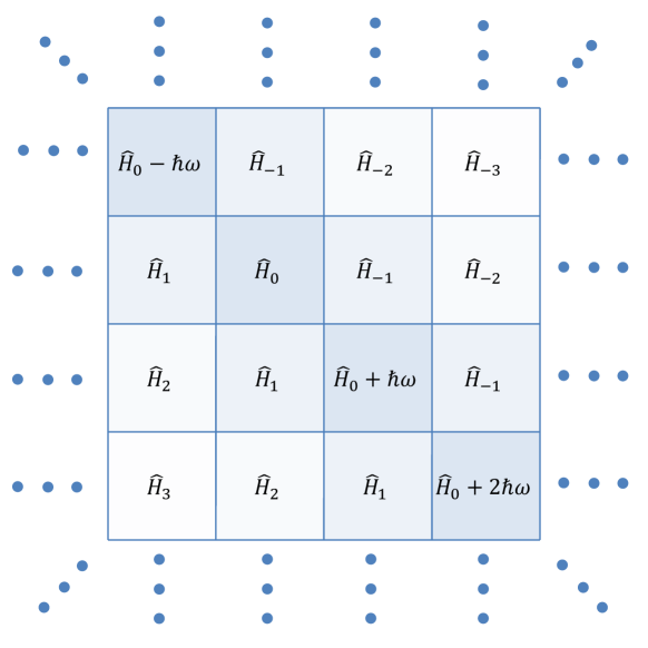
From this restricted class of basis states all possible sets of basis states can now be constructed by applying unitary operators $\bar{U}$, $|\alpha m\rangle\!\rangle_{U}=\bar{U}|\alpha m\rangle\!\rangle$. With respect to the basis $|\alpha m\rangle\!\rangle$ the quasienergy operator possesses the matrix elements

$$\langle\!\langle\alpha^{\prime}m^{\prime}|\bar{Q}|\alpha m\rangle\!\rangle = \frac{1}{T}\int_{0}^{T}\!\mathrm{d}t\,e^{-im^{\prime}\omega t}\langle\alpha^{\prime}|\hat{H}(t)-i\hbar\mathrm{d}_{t}|\alpha\rangle e^{im\omega t}$$ (22)

$$= \langle\alpha^{\prime}|\hat{H}_{m^{\prime}-m}|\alpha\rangle+\delta_{m^{\prime}m}\delta_{\alpha^{\prime}\alpha}m\hbar\omega,$$

where

$$\hat{H}_{m}=\frac{1}{T}\int_{0}^{T}\!\mathrm{d}t\,e^{-im\omega t}\hat{H}(t)=\hat{H}_{-m}^{\dagger}$$ (23)

is the Fourier transform of the Hamiltonian $\hat{H}(t)$, such that $\hat{H}(t)=\sum_{m=-\infty}^{\infty}e^{im\omega t}\hat{H}_{m}$. With respect to the Fourier indices $m$ the quasienergy operator possesses the transparent block structure depicted in Fig. 1. Each block represents an operator $\hat{Q}_{m^{\prime}m}=\hat{H}_{m^{\prime}-m}+\delta_{m^{\prime}m}m\hbar\omega$ acting in $\mathcal{H}$.

The structure of the quasienergy operator $\bar{Q}$ resembles that of the Hamiltonian describing a quantum system with Hilbert space $\mathcal{H}$ coupled to a photon-like mode in the classical limit of large photon numbers, where the spectrum becomes periodic in energy. In this picture $m$ plays the role of a relative photon number. The quasienergy eigenvalue problem (20) is, thus, closely related to the dressed-atom picture [52, 53] for a quantum system driven by coherent radiation [54]. Based on this analogy, one often uses the jargon to call $m$ the “photon” number. Moreover, the matrix elements of $\hat{H}_{m}$ are said to describe $m$-“photon” processes. This terminology suggests a very intuitive picture for the physics of time-periodically driven quantum systems and is also employed when the system is actually not driven by a photon mode.

In order to diagonalize or block diagonalize the quasienergy operator, it is natural and sufficient to consider unitary operators $\bar{U}$ that are translationally invariant with respect to the photon index $m$, $\langle\!\langle\alpha^{\prime}m^{\prime}|\bar{U}|\alpha m\rangle\!\rangle=\langle\alpha^{\prime}|\hat{U}_{m^{\prime}-m}|\alpha\rangle$. They correspond to time-periodic unitary operators $\hat{U}(t)=\sum_{m=-\infty}^{\infty}e^{im\omega t}\hat{U}_{m}$ acting in $\mathcal{H}$ (see also B). From Eq. (19) we can infer that a unitary transformation with such an operator $\bar{U}$,

$$\bar{Q} \to \bar{Q}^{\prime}=\bar{U}^{\dagger}\bar{Q}\bar{U}$$

$$|u\rangle\!\rangle \to |u^{\prime}\rangle\!\rangle=\bar{U}^{\dagger}|u\rangle\!\rangle,$$ (24)

is equivalent to a gauge transformation

$$\hat{H}(t) \to \hat{H}^{\prime}(t)=\hat{U}^{\dagger}(t)\hat{H}(t)\hat{U}(t)-i\hbar\hat{U}^{\dagger}(t)\mathrm{d}_{t}\hat{U}(t)$$

$$|\psi(t)\rangle \to |\psi^{\prime}(t)\rangle=\hat{U}^{\dagger}(t)|\psi(t)\rangle.$$ (25)

with a time-periodic unitary operator $\hat{U}(t)$. Accordingly, the matrix elements of the transformed quasienergy operator

$$\langle\!\langle\alpha^{\prime}m^{\prime}|\bar{Q}^{\prime}|\alpha m\rangle\!\rangle=\langle\alpha^{\prime}|\hat{H}_{m^{\prime}-m}^{\prime}|\alpha\rangle+\delta_{m^{\prime}m}\delta_{\alpha^{\prime}\alpha}m\hbar\omega,$$ (26)

are determined by the Fourier components $\hat{H}_{m}^{\prime}=\frac{1}{T}\int_{0}^{T}\!\mathrm{d}t\,e^{-im\omega t}\hat{H}^{\prime}(t)$ of the gauge-transformed Hamiltonian.

The unitary operator $\bar{U}_{D}$ that diagonalizes the quasienergy operator with respect to a certain basis $|\alpha m\rangle\!\rangle$,

$$\langle\!\langle\alpha^{\prime}m^{\prime}|\bar{U}_{D}^{\dagger}\bar{Q}\bar{U}_{D}|\alpha m\rangle\!\rangle=\delta_{m^{\prime}m}\delta_{\alpha^{\prime}\alpha}(\langle\alpha|\hat{H}_{D}|\alpha\rangle+m\hbar\omega)$$ (27)

is constructed such that it leads to a time-independent gauge-transformed Hamiltonian

$$\hat{H}_{D}=\hat{U}_{D}^{\dagger}(t)\hat{H}(t)\hat{U}_{D}(t)-i\hbar\hat{U}_{D}^{\dagger}(t)\mathrm{d}_{t}\hat{U}_{D}(t)$$ (28)

that is diagonal with respect to the basis states $|\alpha\rangle$,

$$\langle\alpha^{\prime}|\hat{H}_{D}|\alpha\rangle=\delta_{\alpha^{\prime}\alpha}\varepsilon_{\alpha}.$$ (29)

The Floquet Hamiltonian $\hat{H}^{F}_{t_{0}}$ is related to $H_{D}$ via the unitary transformation

$$\hat{H}^{F}_{t_{0}}=\hat{U}_{D}(t_{0})\hat{H}_{D}\hat{U}_{D}^{\dagger}(t_{0}).$$ (30)

The Floquet mode $|u_{\alpha m}\rangle\!\rangle=\bar{U}_{D}|\alpha m\rangle\!\rangle$ with quasienergy $\varepsilon_{\alpha m}=\varepsilon_{\alpha}+m\hbar\omega$ reads $|u_{\alpha m}(t)\rangle=\hat{U}_{D}(t)|\alpha\rangle e^{im\omega t}$, so that the micromotion operator can be expressed like

$$\hat{U}_{F}(t,t^{\prime})=\hat{U}_{D}(t)\hat{U}_{D}^{\dagger}(t^{\prime}).$$ (31)

3 Block diagonalization of the quasienergy operator and effective Hamiltonian

Figure 2: By block diagonalization of the quasienergy operator with respect to the photon index $m$, one obtains the effective Hamiltonian $\hat{H}_{F}$.

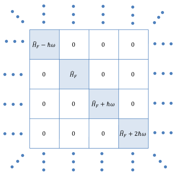
The quasienergy eigenvalue problem (20) is a convenient starting point for computing the Floquet Hamiltonian and the micromotion operator directly, without the need to compute the Floquet modes and their quasienergies. For this purpose one does not need to fully diagonalize the quasienergy operator. Instead one has to find a unitary operator $\bar{U}_{F}$ that block diagonalizes the quasienergy operator with respect to the “photon” index $m$,

$$\langle\!\langle\alpha^{\prime}m^{\prime}|\bar{U}^{\dagger}_{F}\bar{Q}\bar{U}_{F}|\alpha m\rangle\!\rangle=\delta_{m^{\prime}m}(\langle\alpha^{\prime}|\hat{H}_{F}|\alpha\rangle+\delta_{\alpha^{\prime}\alpha}m\hbar\omega),$$ (32)

as illustrated in Fig. 2. Here we have introduced the gauge-transformed Hamiltonian

$$\hat{H}_{F}=\hat{U}^{\dagger}_{F}(t)\hat{H}(t)\hat{U}_{F}(t)-i\hbar\hat{U}^{\dagger}_{F}(t)\mathrm{d}_{t}\hat{U}_{F}(t),$$ (33)

which by construction is time independent. In fact, choosing an operator $\bar{U}_{F}$ that block diagonalizes the quasienergy operator is equivalent to choosing $\hat{U}_{F}(t)$ such that the gauge transformation (33) leads to a time-independent Hamiltonian $\hat{H}_{F}$. This time-independent Hamiltonian $\hat{H}_{F}$ is called effective Hamiltonian. Note that the unitary operator $\bar{U}_{F}$ is not determined uniquely. For example, multiplying $\hat{U}_{F}(t)$ with any time-independent unitary operator from the right leads to a mixing of states within the diagonal blocks of $\bar{U}^{\dagger}_{F}\bar{Q}\bar{U}_{F}$, but does not destroy the block diagonal form. Unlike the operator $\bar{U}_{D}$ that diagonalizes the quasienergy operator, $\bar{U}_{F}$ does not depend on the basis states $|\alpha\rangle$.

Now, each of the diagonal blocks of $\bar{U}^{\dagger}_{F}\bar{Q}\bar{U}_{F}$ represents a possible choice for the Floquet Hamiltonian. This can be seen by writing the quasienergy operator like $\bar{Q}=\sum_{m=-\infty}^{\infty}\sum_{n}|u_{nm}\rangle\!\rangle(\varepsilon_{\alpha}+m\hbar\omega)\langle\!\langle u_{nm}|$ and comparing it to the representation (9) of the Floquet Hamiltonian. From the $m=m^{\prime}=0$ block one obtains

$$\hat{H}^{F}_{t_{0}} = \sum_{\alpha^{\prime}\alpha}|\alpha^{\prime}0(t_{0})\rangle_{F}\,{}_{F}\langle\!\langle\alpha^{\prime}0|\bar{Q}|\alpha 0\rangle\!\rangle_{F}\,{}_{F}\langle\alpha 0(t_{0})|$$ (34)

$$= \sum_{\alpha^{\prime}\alpha}\hat{U}_{F}(t_{0})|\alpha^{\prime}\rangle\,\langle\!\langle\alpha^{\prime}0|\bar{U}_{F}^{\dagger}\bar{Q}\bar{U}_{F}|\alpha 0\rangle\!\rangle\,\langle\alpha|\hat{U}_{F}^{\dagger}(t_{0})$$

$$= \hat{U}_{F}(t_{0})\hat{H}_{F}\hat{U}_{F}^{\dagger}(t_{0}),$$

where we have defined the rotated basis states

$$|\alpha m\rangle\!\rangle_{F}\equiv\bar{U}_{F}|\alpha m\rangle\!\rangle$$ (35)

and used Eq. (32). We can see that the Floquet Hamiltonian $\hat{H}^{F}_{t_{0}}$ is equivalent to the effective Hamiltonian $\hat{H}_{F}$ in the sense that both are related to each other by a unitary transformation. Moreover, we can use the unitary operator $\bar{U}_{F}$ to construct the micromotion operator:

$$\hat{U}_{F}(t,t^{\prime})=\hat{U}_{F}(t)\hat{U}_{F}^{\dagger}(t^{\prime}).$$ (36)

From $\hat{H}^{F}_{t}$ and $\hat{U}_{F}(t,t^{\prime})$ one can then directly obtain the time evolution operator using Eq. (12).

However, the time evolution operator $\hat{U}(t_{2},t_{1})$ can also be expressed directly in terms of $\hat{H}_{F}$ and $\hat{U}_{F}(t)$ without introducing $\hat{H}^{F}_{t_{0}}$ and $\hat{U}_{F}(t^{\prime},t)$. Namely [42],

$$\hat{U}(t_{2},t_{1})=\hat{U}_{F}(t_{2})e^{-\frac{i}{\hbar}(t_{2}-t_{1})\hat{H}_{F}}\hat{U}_{F}^{\dagger}(t_{1}).$$ (37)

Compared to the representation (12) of the time-evolution operator in terms of the Floquet Hamiltonian $\hat{H}^{F}_{t_{0}}$ and the micromotion operator $\hat{U}_{F}(t_{2},t_{1})$, this expression has the disadvantage that it is a product of three operators and not just of two. However, using the representation (37) has also advantages. The micromotion has been expressed by the one-point micromotion operator $\hat{U}_{F}(t)$, instead of by the two-point operator $\hat{U}_{F}(t,t^{\prime})$, and the phase evolution is described by an effective Hamiltonian $\hat{H}_{F}$ without the parametric dependence on the switching time $t_{0}$ of $\hat{H}^{F}_{t_{0}}$. The micromotion operator $\hat{U}_{F}(t)$ can also be expressed like

$$\hat{U}_{F}(t)=\exp\big{(}\hat{G}(t)\big{)}$$ (38)

in terms of an anti-hermitian operator $\hat{G}=-\hat{G}^{\dagger}$. The hermitian operator $\hat{K}(t)=i\hat{G}(t)$ has recently been given the intuitive name kick operator [43].

The diagonalization of the effective Hamiltonian $\hat{H}_{F}$,

$$\hat{H}_{F}|\tilde{u}_{n}\rangle=\varepsilon_{n}|\tilde{u}_{n}\rangle,$$ (39)

provides the Floquet modes and their quasienergies:

$$|u_{nm}(t)\rangle = \hat{U}_{F}(t)|\tilde{u}_{n}\rangle e^{im\omega t},$$ (40)

$$\varepsilon_{nm} = \varepsilon_{n}+m\hbar\omega.$$ (41)

Thus, the Floquet modes $|u_{n}(t)\rangle\equiv|u_{n0}(t)\rangle$, which describe the micromotion, are superpositions

$$|u_{n}(t)\rangle=\sum_{\alpha}\gamma_{\alpha n}|\alpha(t)\rangle_{F}.$$ (42)

of the time-dependent basis states

$$|\alpha(t)\rangle_{F}=\hat{U}_{F}(t)|\alpha 0\rangle=\hat{U}_{F}(t)|\alpha\rangle,$$ (43)

with time-independent coefficients

$$\gamma_{\alpha n}=\langle\alpha|\tilde{u}_{n}\rangle.$$ (44)

The strategy of computing the effective Hamiltonian directly, without computing the Floquet states before, separates the Floquet problem into two distinct subproblems related to the short-time and the long-time dynamics, respectively. The first problem, computing the effective Hamiltonian (as well as the micromotion operator), concerns the short-time dynamics within one driving period only. The second problem consists in the integration of the time evolution generated by the effective Hamiltonian for a given initial state or even in the complete diagonalization of the effective Hamiltonian. This separation allows to address the long-time dynamics over several driving periods in a very efficient way, without the need to follow the details of the dynamics within every driving period.

The advantage of splitting the Floquet problem into two parts becomes apparent especially when one of the two problems is more difficult than the other. A simple example for a case where computing the effective Hamiltonian is more difficult than diagonalizing it, is a periodically driven two-level system corresponding to a spin-1/2 degree of freedom. While the block diagonalization of the quasienergy operator can generally not be accomplished analytically, the effective Hamiltonian describes (like every time-independent $2\times 2$ Hamiltonian) a spin 1/2 in a constant magnetic field leading to a simple precession dynamics on the Bloch sphere. Thus, once the effective Hamiltonian and the micromotion operator are computed, the time evolution is known. An example for the opposite case, where the effective Hamiltonian can be computed at least approximately while its diagonalization is much harder, is a time-periodically driven Hubbard-type model [19]. It describes interacting particles on a tigh-binding lattice. This driven model allows for a quantitative description of experiments with ultracold atoms in optical lattices. In the limit of high-frequency forcing a suitable analytical approximation to the effective Hamiltonian can be well justified on the time scale of a typical optical lattice experiment. However, the effective Hamiltonian will constitute a many-body problem that is difficult to solve.

The possibility to compute the effective Hamiltonian for a many-body lattice system, at least within a suitable approximation, is also the basis for a novel and powerful type of quantum engineering. Here the properties of the effective Hamiltonian $\hat{H}_{F}$ are tailored by engineering the periodic time dependence of the Hamiltonian $\hat{H}(t)$. This Floquet engineering has recently been successfully applied to ultracold atomic quantum gases (see references in the introduction). The fact that the effective Hamiltonian can possess properties that are hard to achieve otherwise, like the coupling of the kinetics of charge-neutral atoms to a vector potential describing an (artificial) magnetic field [30, 31, 34, 35, 36, 37, 28, 55, 56, 32, 27, 57, 58, 59, 38, 39, 60], makes Floquet engineering also interesting for quantum simulation. Here, a quantum mechanical many-body model is realized accurately in the laboratory in order to investigate its properties by doing experiments. An essential prerequiste for Floquet engineering is an accurate approximation to the effective Hamiltonian. In the next section we will systematically derive a high-frequency approximation to both the effective Hamiltonian and the micromotion operator by block diagonalizing the quasienergy operator by means of degenerate perturbation theory.

4 High-frequency expansion from degenerate perturbation theory

Degenerate perturbation theory is a standard approximation scheme for the systematic block diagonalization of a hermitian operator into two subspaces—a subspace of special interest on the one hand and the rest of state space on the other—that are divided by a large spectral gap. Here we adapt the method such that it allows for a systematic block diagonalization of the quasienergy operator with respect to the “photon” index $m$ (C). Moreover, we will identify the system-independent “photonic” part $-i\hbar\mathrm{d}_{t}$ of the quasienergy operator (19), with $\langle\!\langle\alpha^{\prime}m^{\prime}|-i\hbar\mathrm{d}_{t}|\alpha m\rangle\!\rangle=\delta_{m^{\prime}m}\delta_{\alpha^{\prime}\alpha}m\hbar\omega$, as the unperturbed problem. As a consequence the system-specific Hamiltonian $\hat{H}(t)$ constitutes the perturbation. This will allow us to systematically derive simple and universal expansions for both the effective Hamiltonian $\hat{H}_{F}$ and the micromotion operator $\hat{U}_{F}(t)$ in the high-frequency limit, where $\hbar\omega$ constitutes a large spectral gap between the unperturbed subspaces (see Fig. 1). We would like to point out that the application of degenerate perturbation theory in the extended Floquet Hilbert space is a well established method. For example, it has recently been employed to estimate the matrix element for the resonant creation of collective excitations in a driven Bose-Hubbard model [51] and to treat a dissipative driven two-level system [61].

The basic strategy of our perturbative approach can be summarized as follows. The quasienergy operator is divided into an unperturbed part $\bar{Q}_{0}$ and a perturbation $\bar{V}$,

$$\bar{Q}=\bar{Q}_{0}+\bar{V}.$$ (45)

The unperturbed operator can be diagonalized and separates the extended Floquet Hilbert space $\mathcal{F}$ into uncoupled subspaces $\mathcal{F}^{(0)}_{m}$ of sharp “photon” numbers $m$ with projectors $\bar{P}_{m}=\sum_{\alpha}|\alpha m\rangle\!\rangle\langle\!\langle\alpha m|$. These subspaces shall be separated by unperturbed spectral gaps of the order of $\hbar\omega$, which are assumed to be large compared to the strength $p$ of the perturbation coupling states of different subspaces. When smoothly switching on the perturbation, such that the spectral gaps do not close, the unperturbed subspaces $\mathcal{F}^{(0)}_{m}$ will be transformed adiabatically to the perturbed subspaces $\mathcal{F}_{m}$ corresponding to a diagonal block of the perturbed problem. Since the perturbation is weak compared to the gap, $\mathcal{F}_{m}$ will differ from $\mathcal{F}^{(0)}_{m}$ by small admixtures of states $\not\in\mathcal{F}^{(0)}_{m}$ only. This admixture will be calculated perturbatively by expanding a unitary operator $\bar{U}_{F}$ that relates the basis states $|\alpha m\rangle\!\rangle$ spanning the unperturbed subpsaces $\mathcal{F}_{m}^{(0)}$ to the basis states $|\alpha m\rangle\!\rangle_{F}=\bar{U}_{F}|\alpha m\rangle\!\rangle$ spanning the perturbed subspaces $\mathcal{F}_{m}$. In contrast, if the spectral gap separating different subspaces would close, arbitrary weak coupling can hybridize degenerate states of different subspaces, contrary to the assumption of a weak perturbative admixture. The general formalism is developed in C and will be applied to a specific choice of the unperturbed problem in the following.

Figure 3: Structure of the quasienergy operator $\bar{Q}=\bar{Q}^{\prime}_{0}+\bar{V}^{\prime}_{D}+\bar{V}^{\prime}_{X}=\bar{Q}_{0}+\bar{V}_{D}+\bar{V}_{X}$, the unperturbed problem is given by $\bar{Q_{0}}^{(^{\prime})}$ and the perturbation $\bar{V}^{(^{\prime})}$ can be separated into a block diagonal part $\bar{V}_{D}^{(^{\prime})}$ that conserves the “photon” number $m$ and a part $\bar{V}_{X}^{(^{\prime})}$ comprising $m\neq 0$-photon processes. (a) Generic choice of the unperturbed operator $\bar{Q}_{0}^{\prime}$. (b) Simple system-independent choice of the unperturbed problem $\hat{Q}_{0}(t)=-i\hbar\mathrm{d}_{t}$ to be used here; all unperturbed states of identical “photon” number $m$ are degenerate.

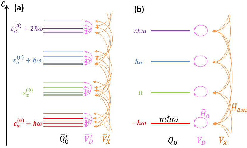
For the procedure described above a general and legitimate choice of the unperturbed problem would consist in the diagonal terms of the quasienergy operator with respect to a conveniently chosen set of basis states $|\alpha,m\rangle\!\rangle$,

$$\bar{Q}^{\prime}_{0} = \sum_{m}\sum_{\alpha}|\alpha m\rangle\!\rangle\langle\!\langle\alpha m|\bar{Q}|\alpha m\rangle\!\rangle\langle\!\langle\alpha m|$$ (46)

$$= \sum_{m}\sum_{\alpha}|\alpha m\rangle\!\rangle(\varepsilon_{\alpha}^{(0)}+m\hbar\omega)\langle\!\langle\alpha m|,$$

with $\varepsilon_{\alpha}^{(0)}=\langle\alpha|\hat{H}_{0}|\alpha\rangle$. The operator $\bar{Q}^{\prime}_{0}$ is diagonal with respect to the basis states $|\alpha m\rangle\!\rangle$ by construction and the corresponding perturbation $\bar{V}^{\prime}=\bar{Q}-\bar{Q}^{\prime}_{0}$ consists of a block-diagonal part $\bar{V}^{\prime}_{D}$ that couples states $|\alpha m\rangle\!\rangle$ and $|\alpha^{\prime}m\rangle\!\rangle$ of the same “photon” number $m$ and a block-off-diagonal part $\bar{V}^{\prime}_{X}$ that couples states $|\alpha m\rangle\!\rangle$ and $|\alpha^{\prime}m^{\prime}\rangle\!\rangle$ of different “photon” numbers $m^{\prime}$ and $m$. The problem to be solved by perturbation theory is visualized in Figure 3(a). The unperturbed problem and the perturbation expansion depend on the choice of the basis states $|\alpha\rangle$.

However, for the sake of simplicity we will not use Eq. (46). Instead we will simplify the unperturbed problem further, reducing it to the “photonic” part of the quasienergy operator,

$$\hat{Q}_{0}(t)=-i\hbar\mathrm{d}_{t},$$ (47)

or

$$\bar{Q}_{0}=\sum_{m}\sum_{\alpha}|\alpha m\rangle\!\rangle m\hbar\omega\langle\!\langle\alpha m|,$$ (48)

which does not depend on the system’s Hamiltonian. For this choice the unperturbed quasienergies are degenerate within each subspace and read $\varepsilon_{\alpha m}^{(0)}=m\hbar\omega$. So $\bar{Q}_{0}$ is diagonal not only with respect to a specific set of basis states, but with respect to any set of basis states of the type $|\alpha m\rangle\!\rangle$. The perturbation is given by the Hamiltonian,

$$\hat{V}(t)=\hat{H}(t)$$ (49)

or

$$\bar{V}=\bar{H}=\sum_{m^{\prime}m}\sum_{\alpha^{\prime}\alpha}|\alpha^{\prime}m^{\prime}\rangle\!\rangle\langle\alpha^{\prime}|\hat{H}_{m^{\prime}-m}|\alpha\rangle\langle\!\langle\alpha m|.$$ (50)

It can be decomposed like

$$\bar{V}=\bar{V}_{D}+\bar{V}_{X}.$$ (51)

Here the block-diagonal part $\bar{V}_{D}$ comprises the $m^{\prime}=m$ terms describing zero-“photon” processes determined by the time-averaged Hamiltonian,

$$\hat{V}_{D} = \hat{H}_{0},$$ (52)

$$\bar{V}_{D} = \sum_{m}\sum_{\alpha^{\prime}\alpha}|\alpha^{\prime}m\rangle\!\rangle\langle\alpha^{\prime}|\hat{H}_{0}|\alpha\rangle\langle\!\langle\alpha m|.$$ (53)

The block-off-diagonal part $\bar{V}_{X}$ describes $\Delta m$-“photon” processes determined by the Fourier components $\hat{H}_{\Delta m}$ of the Hamiltonian,

$$\hat{V}_{X}(t) = \sum_{\Delta m\neq 0}e^{i\Delta m\omega t}\hat{H}_{\Delta m}$$ (54)

$$\bar{V}_{X} = \sum_{m}\sum_{\Delta m\neq 0}\sum_{\alpha^{\prime}\alpha}|\alpha^{\prime}m+\Delta m\rangle\!\rangle\langle\alpha^{\prime}|\hat{H}_{\Delta m}|\alpha\rangle\langle\!\langle\alpha m|.$$ (55)

The problem is visualized in Figure 3(b). Its simple structure will allow us to write down universal analytical expressions for the leading terms of a perturbative high-frequency expansion of the effective Hamiltonian and the micromotion operator in powers of $p/\hbar\omega$, with $p$ symbolizing the perturbation strength.

Before moving on, we note in passing that it can be useful to shift the “photon” number of an unperturbed state $|\alpha m\rangle\!\rangle$ by some integer $\Delta m$, before applying the high-frequency approximation. Such a procedure can be useful, if two states $|\alpha_{1}\rangle$ and $|\alpha_{2}\rangle$ have time-averaged energies $\varepsilon^{(0)}_{\alpha}=\langle\alpha|\hat{H}_{0}|\alpha\rangle$ that are separated by $\Delta m$ “photon” energies of $\hbar\omega$, so that $\varepsilon^{(0)}_{\alpha_{2}}-\varepsilon^{(0)}_{\alpha_{1}}=\Delta m\hbar\omega+\delta$ with $\delta\ll\hbar\omega$. In this case the two unperturbed basis states $|\alpha_{1}m\rangle\!\rangle$ and $|\alpha_{2}m\rangle\!\rangle$, which are degenerate with respect to the unperturbed quasienergy operator, have average quasienergies $\langle\!\langle\alpha m|\bar{Q}|\alpha m\rangle\!\rangle=\varepsilon^{(0)}_{\alpha}+m\hbar\omega$ that are also separated by the large distance $\Delta m\hbar\omega+\delta$. Obviously, this violates the requirement that the perturbation should be weak. In turn the states $|\alpha_{1}m\rangle\!\rangle$ and $|\alpha_{2}(m-\Delta m)\rangle\!\rangle$ have average quasienergies that are nearly degenerate. Thus it is useful to redefine the “photon” number of states with quantum number $\alpha_{2}$, so that $|\alpha_{2}m\rangle\!\rangle^{\prime}=|\alpha_{2}(m-\Delta m)\rangle\!\rangle$. This redefinition is equivalent to a gauge transformation (2.3) in $\mathcal{H}$, where the unitary operator $e^{-i\Delta m\omega t}|\alpha_{2}\rangle\langle\alpha_{2}|$ is employed to shift the time-averaged energy of $|\alpha_{2}\rangle$ by $-\Delta m\hbar\omega$. After this transformation the high-frequency approximation can be applied and used to describe the resonant coupling between both states $|\alpha_{1}\rangle$ and $|\alpha_{2}\rangle$. Such a procedure can be employed, e.g., to describe resonant “photon”-assisted (or AC-induced) tunneling against a strong potential gradient [12, 45].

4.1 Micromotion

We wish to compute the unitary operator $\bar{U}_{F}$ that relates the unperturbed basis states $|\alpha m\rangle\!\rangle$ to the perturbed basis states $|\alpha m\rangle\!\rangle_{F}$ that block diagonalize the quasienergy operator in a perturbative fashion. In the canonical van Vleck degenerate perturbation theory, it is written like

$$\bar{U}_{F}=\exp(\bar{G}),$$ (56)

with anti-hermitian operator

$$\bar{G}=-\bar{G}^{\dagger}.$$ (57)

In order to minimize the mixing of unperturbed states belonging to the same unperturbed subspace, it is, moreover, required that $\bar{G}$ is block off diagonal. One can now systematically expand $\bar{G}$ like

$$\bar{G}=\sum_{\nu=1}^{\infty}\bar{G}^{(\nu)}$$ (58)

in powers of the perturbation. The general formalism for the perturbative expansion of $\bar{G}$ in a situation where the state space is partitioned into more than just two subspaces is described in C. Differences with respect to the standard procedure, where the state space is just bipartitioned, arise as a consequence of the fact that for multipartitioning it is generally not true anymore that the product of two block-off-diagonal operators is block diagonal.

The general form of the leading terms of the expansion (58) is given by Eqs. (232) and (236) of C. Let us evaluate them for the particular choice of the unperturbed problem (47). Apart from

$$\langle\!\langle\alpha^{\prime}m|\bar{G}^{(\nu)}|\alpha m\rangle\!\rangle=0,$$ (59)

for all diagonal matrix elements, following directly from $\bar{G}$ being block-off-diagonal, for $m^{\prime}\neq m$ we obtain

$$\langle\!\langle\alpha^{\prime}m^{\prime}|\bar{G}^{(1)}|\alpha m\rangle\!\rangle=-\frac{\langle\alpha^{\prime}|\hat{H}_{m^{\prime}-m}|\alpha\rangle}{(m^{\prime}-m)\hbar\omega}$$ (60)

and

$$\langle\!\langle\alpha^{\prime}m^{\prime}|\bar{G}^{(2)}|\alpha m\rangle\!\rangle = \frac{\langle\alpha^{\prime}|\big{[}\hat{H}_{0},\hat{H}_{m^{\prime}-m}\big{]}|\alpha\rangle}{[(m^{\prime}-m)\hbar\omega]^{2}}$$ (61)

$$+\,\frac{1}{2}\sum_{m^{\prime\prime}\neq m,m^{\prime}}\frac{\langle\alpha^{\prime}|\hat{H}_{m^{\prime}-m^{\prime\prime}}\hat{H}_{m^{\prime\prime}-m}|\alpha\rangle}{(m^{\prime}-m)\hbar\omega}$$

$$\times\bigg{[}\frac{1}{(m^{\prime\prime}-m^{\prime})\hbar\omega}+\frac{1}{(m^{\prime\prime}-m)\hbar\omega}\bigg{]}.$$

We can now also expand the unitary operator $\bar{U}_{F}$ in powers of the perturbation,

$$\bar{U}_{F}=\sum_{\nu=1}^{\infty}\bar{U}_{F}^{(\nu)}.$$ (62)

One finds

$$\bar{U}_{F}^{(0)} = 1,$$ (63)

$$\bar{U}_{F}^{(1)} = \bar{G}^{(1)},$$ (64)

$$\bar{U}_{F}^{(2)} = \bar{G}^{(2)}+\frac{1}{2}\big{[}\bar{G}^{(1)}\big{]}^{2},$$ (65)

where the second term of the last equation possesses matrix elements

$$\langle\alpha^{\prime}m^{\prime}|\frac{1}{2}\big{[}\bar{G}^{(1)}\big{]}^{2}|\alpha m\rangle\!\rangle=\sum_{m^{\prime\prime}\neq m,m^{\prime}}\frac{\langle\alpha^{\prime}|\hat{H}_{m^{\prime}-m^{\prime\prime}}\hat{H}_{m^{\prime\prime}-m}|\alpha\rangle}{(m^{\prime}-m^{\prime\prime})(m^{\prime\prime}-m)(\hbar\omega)^{2}},$$ (66)

which are finite also for $m^{\prime}=m$.

The corresponding operators in $\mathcal{H}$ can be constructed by employing the relation

$$\hat{A}(t)=\sum_{m}e^{im^{\prime}\omega t}|\alpha^{\prime}\rangle\langle\!\langle\alpha^{\prime}m^{\prime}|\bar{A}|\alpha 0\rangle\!\rangle\langle\alpha|$$ (67)

that is valid for operators $\bar{A}$ that are translationally invariant with respect to the “photon” number, $\langle\!\langle\alpha^{\prime}m+\Delta m|\bar{A}|\alpha m\rangle\!\rangle=\langle\!\langle\alpha\Delta m|\bar{A}|\alpha 0\rangle\!\rangle$. In doing so, $\bar{U}_{F}$ and $\bar{G}$ translate into time periodic operators $\hat{U}_{F}(t)$ and $\hat{G}(t)$ and Eq. (56) into

$$\hat{U}_{F}(t)\equiv\exp(\hat{G}(t))$$ (68)

(see also B). The leading terms of the perturbation expansion take the form

$$\hat{G}^{(1)}(t) = -\sum_{m\neq 0}\frac{e^{im\omega t}}{m\hbar\omega}\hat{H}_{m}\,,$$ (69)

$$\hat{G}^{(2)}(t) = \sum_{m\neq 0}\Bigg{\{}\frac{e^{im\omega t}\big{[}\hat{H}_{0},\hat{H}_{m}\big{]}}{(m\hbar\omega)^{2}}+\frac{1}{2}\sum_{m^{\prime}\neq 0,m}\frac{e^{i(m-m^{\prime})\omega t}\big{[}\hat{H}_{-m^{\prime}},\hat{H}_{m}\big{]}}{m(m-m^{\prime})(\hbar\omega)^{2}}\Bigg{\}}$$

and

$$\hat{U}_{F}^{(0)}(t) = 1,$$ (71)

$$\hat{U}_{F}^{(1)}(t) = \hat{G}^{(1)}(t),$$ (72)

$$\hat{U}_{F}^{(2)}(t) = \hat{G}^{(2)}(t)+\frac{1}{2}\sum_{m\neq 0}\sum_{m^{\prime}\neq 0}\frac{e^{i(m+m^{\prime})\omega t}\hat{H}_{m^{\prime}}\hat{H}_{m}}{m^{\prime}m(\hbar\omega)^{2}}.$$ (73)

One can express these terms also as time integrals. For the leading order we obtain

$$\hat{G}^{(1)}(t)=\hat{U}_{F}^{(1)}(t) = -\frac{1}{T}\int_{t_{0}}^{t_{0}+T}\!\mathrm{d}t^{\prime}\,\hat{H}(t^{\prime})\sum_{m=1}^{\infty}\frac{2i\sin(m\omega(t-t^{\prime}))}{m\hbar\omega}$$ (74)

$$= -\frac{i\pi}{\hbar\omega}\frac{1}{T}\int_{t}^{t+T}\!\mathrm{d}t^{\prime}\,\hat{H}(t^{\prime})\Big{(}1-2\frac{t-t^{\prime}}{T}\Big{)}.$$

In the final result we have separated a factor of $\frac{1}{T}$ representing the inverse integration time. It was obtained by setting the free parameter $t_{0}$ to $t_{0}=t$ allowing us to use

$$\sum_{k=1}^{\infty}\frac{\sin(kx)}{k}=\frac{\pi-x}{2}\qquad\mathrm{for}\qquad 0<x<2\pi,$$ (75)

which is formula 1.441-1 of reference [62].

One can now approximate $\hat{U}_{F}(t)$ up to a finite order $\tilde{\nu}$ by simply truncating the perturbative expansion of $\hat{U}_{F}(t)$ like $\hat{U}_{F}(t)\approx\sum_{\nu=0}^{\tilde{\nu}}\hat{U}_{F}^{(\nu)}(t)$. However, this approximation has the disadvantage that it does not preserve unitarity at any finite order $\tilde{\nu}$. In turn, truncating the expansion of $\hat{G}(t)$ leads to an approximation

$$\hat{U}_{F}(t)\approx\exp\bigg{(}\sum_{\nu=1}^{\tilde{\nu}}\hat{G}^{(\nu)}\bigg{)}\equiv\hat{U}^{[\tilde{\nu}]}_{F}(t)$$ (76)

that gives rise to a unitary operator $\hat{U}^{[\tilde{\nu}]}_{F}(t)$ for every finite $\tilde{\nu}$.

The unitary two-point micromotion operator can be written like

$$\hat{U}_{F}(t,t^{\prime})=\hat{U}_{F}(t)\hat{U}_{F}^{\dagger}(t^{\prime})\equiv\exp\big{(}\hat{F}(t,t^{\prime})\big{)}$$ (77)

with anti-hermitian operator $\hat{F}(t,t^{\prime})=-\hat{F}^{\dagger}(t,t^{\prime})$. Expanding $\hat{F}(t,t^{\prime})$ in powers of the perturbation,

$$\hat{F}(t,t^{\prime})=\sum_{\nu=1}^{\infty}\hat{F}^{(\nu)}(t,t^{\prime}),$$ (78)

and comparing the epxansion of $\exp\big{(}\hat{F}(t,t^{\prime})\big{)}$ in powers of the perturbation with that of $\exp\big{(}\hat{G}(t)\big{)}\exp\big{(}-\hat{G}(t^{\prime})\big{)}$, one can identify

$$\hat{F}^{(1)}(t,t^{\prime}) = \hat{G}^{(1)}(t)-\hat{G}^{(1)}(t^{\prime}),$$ (79)

$$\hat{F}^{(2)}(t,t^{\prime}) = \hat{G}^{(2)}(t)-\hat{G}^{(2)}(t^{\prime})-\frac{1}{2}\big{[}\hat{G}^{(1)}(t),\hat{G}^{(1)}(t^{\prime})\big{]},$$ (80)

and so on. This gives the explicit expressions for the leading orders

$$\hat{F}^{(1)}(t,t^{\prime}) = -\sum_{m\neq 0}\frac{1}{m\hbar\omega}\bigg{(}e^{im\omega t}-e^{im\omega t^{\prime}}\bigg{)}\hat{H}_{m},$$ (81)

$$\hat{F}^{(2)}(t,t^{\prime}) = \sum_{m\neq 0}\Bigg{\{}\frac{\Big{(}e^{im\omega t}-e^{im\omega t^{\prime}}\Big{)}\big{[}\hat{H}_{0},\hat{H}_{m}\big{]}}{(m\hbar\omega)^{2}}$$ (82)

$$+\,\frac{1}{2}\sum_{m^{\prime}\neq 0,m}\frac{\Big{(}e^{i(m-m^{\prime})\omega t}-e^{i(m-m^{\prime})\omega t^{\prime}}\Big{)}\big{[}\hat{H}_{-m^{\prime}},\hat{H}_{m}\big{]}}{m(m-m^{\prime})(\hbar\omega)^{2}}\Bigg{\}}$$

$$-\,\frac{1}{2}\sum_{m\neq 0}\sum_{m^{\prime}\neq 0}\frac{e^{im\omega t-im^{\prime}\omega t^{\prime}}\big{[}\hat{H}_{-m^{\prime}},\hat{H}_{m}\big{]}}{mm^{\prime}(\hbar\omega)^{2}}.$$

An approximation preserving the unitarity of the micromotion operator reads

$$\hat{U}_{F}(t,t^{\prime})\approx\exp\bigg{(}\sum_{\nu=1}^{\tilde{\nu}}\hat{F}^{(\nu)}(t,t^{\prime})\bigg{)}\equiv\hat{U}^{[\tilde{\nu}]}_{F}(t,t^{\prime}).$$ (83)

4.2 Effective Hamiltonian

In order to obtain the effective Floquet Hamiltonian from Eq. (34), we need to compute the matrix elements (32) for $m=m^{\prime}=0$,

$$H^{F}_{\alpha^{\prime}\alpha}\equiv\langle\alpha^{\prime}|\hat{H}_{F}|\alpha\rangle=\langle\!\langle\alpha^{\prime}0|\bar{U}_{F}^{\dagger}\bar{Q}\bar{U}_{F}|\alpha 0\rangle\!\rangle=Q_{0,\alpha^{\prime}\alpha}.$$ (84)

Expanding these matrix elements in powers of the perturbation, the leading terms $Q_{0,\alpha^{\prime}\alpha}^{(\nu)}$ are given by Eqs. (248), (249), (253), and (262) of C. Evaluating these expressions for the unperturbed problem (47), we obtain the perturbative expansion for the effective Hamiltonian

$$\hat{H}_{F}=\sum_{\nu=0}^{\infty}\hat{H}^{(\nu)}_{F},$$ (85)

with $\hat{H}^{(\nu)}_{F}=\sum_{\alpha^{\prime}\alpha}|\alpha^{\prime}\rangle Q_{0,\alpha^{\prime}\alpha}^{(\nu)}\langle\alpha|$. The leading terms are given by

$$\hat{H}_{F}^{(0)} = 0,$$ (86)

$$\hat{H}_{F}^{(1)} = \hat{H}_{0},$$ (87)

$$\hat{H}_{F}^{(2)} = \sum_{m\neq 0}\frac{\hat{H}_{m}\hat{H}_{-m}}{m\hbar\omega},$$ (88)

$$\hat{H}_{F}^{(3)} = \sum_{m\neq 0}\Bigg{(}\frac{\big{[}\hat{H}_{-m},\big{[}\hat{H}_{0},\hat{H}_{m}\big{]}\big{]}}{2(m\hbar\omega)^{2}}+\sum_{m^{\prime}\neq 0,m}\frac{\big{[}\hat{H}_{-m^{\prime}},\big{[}\hat{H}_{m^{\prime}-m},\hat{H}_{m}\big{]}\big{]}}{3mm^{\prime}(\hbar\omega)^{2}}\Bigg{)}.$$

One can express these terms also in terms of time integrals. The leading order is given by the time-averaged Hamiltonian,

$$\hat{H}_{F}^{(1)}=\frac{1}{T}\int_{0}^{T}\!\mathrm{d}t\,\hat{H}(t).$$ (90)

The first correction takes the form

$$\hat{H}_{F}^{(2)} = \frac{1}{T^{2}}\int_{0}^{T}\!\mathrm{d}t_{1}\int_{0}^{T}\!\mathrm{d}t_{2}\,\sum_{m\neq 0}\frac{e^{-im\omega(t_{1}-t_{2})}}{m\hbar\omega}\hat{H}(t_{1})\hat{H}(t_{2})$$ (91)

$$= \frac{1}{T^{2}}\int_{0}^{T}\!\mathrm{d}t_{1}\int_{0}^{t_{1}}\!\mathrm{d}t_{2}\,\sum_{m\neq 0}\frac{e^{-im\omega(t_{1}-t_{2})}}{m\hbar\omega}\big{[}\hat{H}(t_{1}),\hat{H}(t_{2})\big{]}$$

$$= \frac{2\pi}{i\hbar\omega}\frac{1}{2T^{2}}\int_{0}^{T}\!\mathrm{d}t_{1}\int_{0}^{t_{1}}\!\mathrm{d}t_{2}\,\Big{(}1-2\frac{t_{1}-t_{2}}{T}\Big{)}\big{[}\hat{H}(t_{1}),\hat{H}(t_{2})\big{]},$$

where the sum over $m$ has been evaluated using Eq. (75) and where we have separated a factor of $1/(2T^{2})$ representing the inverse integration area. In $\tilde{\nu}$th order the effective Hamiltonian is approximated by

$$\hat{H}_{F}\approx\sum_{\nu=0}^{\tilde{\nu}}\hat{H}^{(\nu)}_{F}\equiv\hat{H}^{[\tilde{\nu}]}_{F}.$$ (92)

The results obtained here via degenerate perturbation theory in the extended Floquet Hilbert space are equivalent to the high-frequency expansion derived in references [42, 43, 44] by different means.

4.3 Role of the driving phase

An important property of the approximation (92) to the effective Hamiltonian is that it is independent of the driving phase. Namely, a shift in time

$$\hat{H}(t)\to\hat{H}^{\prime}(t)=\hat{H}(t-t^{\prime}),$$ (93)

which leads to

$$\hat{H}_{m}\to\hat{H}^{\prime}_{m}=e^{-im\omega t^{\prime}}\hat{H}_{m},$$ (94)

does not alter the perturbation expansion of $\hat{H}_{F}$,

$$\hat{H}_{F}^{(\nu)}\to\hat{H}_{F}^{{}^{\prime}(\nu)}=\hat{H}_{F}^{(\nu)}.$$ (95)

This is ensured by the structure of the perturbation theory, which restricts the products $\hat{H}_{m_{1}}\hat{H}_{m_{2}}\cdots\hat{H}_{m_{\nu}}$ that contribute to $\hat{H}_{F}^{(\nu)}$ to those with $m_{1}+m_{2}+\cdots m_{\nu}=0$. As an immediate consequence, also the approximate quasienergy spectrum, obtained from the diagonalization of $\hat{H}_{F}$, does not acquire a spurious dependence on the driving phase. In this respect, the high-frequency approximation obtained by truncating the high-frequency expansion of $\hat{H}_{F}$ at finite order, Eqs. (76) and (92), is consistent with Floquet theory.

A time shift does, however, modify the terms of the unitary operator $\hat{U}_{F}(t)$ in the expected way,

$$\hat{U}^{(\nu)}_{F}(t)\to\hat{U}^{{}^{\prime}(\nu)}_{F}(t)=\hat{U}^{(\nu)}_{F}(t-t^{\prime}),$$ (96)

since

$$\hat{G}^{(\nu)}(t)\to\hat{G}^{{}^{\prime}(\nu)}(t)=\hat{G}^{(\nu)}(t-t^{\prime}).$$ (97)

4.4 Quasienergy spectrum and Floquet modes

From the approximate Floquet Hamiltonian one can now compute the quasienergy spectrum and the Floquet modes by solving the eigenvalue problem

$$\hat{H}_{F}^{[{\nu}]}|\tilde{u}_{n}\rangle^{[{\nu}]}=\varepsilon^{[{\nu}]}|\tilde{u}_{n}\rangle^{[{\nu}]}.$$ (98)

One obtains

$$\varepsilon_{n}\approx\varepsilon_{n}^{[{\nu}]}$$ (99)

and

$$|u_{n}(t)\rangle\approx\hat{U}_{F}^{[{\nu}^{\prime}]}|u_{n}(t)\rangle^{[\nu]}\equiv|u_{n}^{[{\nu}^{\prime},{\nu}]}(t)\rangle.$$ (100)

Here we have allowed that the order ${\nu}^{\prime}$ of the approximate unitary operator $\hat{U}_{F}^{[\nu^{\prime}]}(t)$ describing the micromotion can be different from the order ${\nu}$ of the approximate Floquet Hamiltonian $\hat{H}_{F}^{[\nu]}$, which determines the Floquet spectrum and the dynamics on longer times. This corresponds to the approximation

$$\hat{H}^{F}_{t_{0}}\approx\hat{U}_{F}^{[{\nu}^{\prime}]}(t_{0})\hat{H}_{F}^{[{\nu}]}\hat{U}_{F}^{[{\nu}^{\prime}]{\dagger}}(t_{0})\equiv\hat{H}^{F[{\nu}^{\prime},{\nu}]}_{t_{0}}.$$ (101)

to the Floquet Hamiltonian $\hat{H}^{F}_{t_{0}}$.

The reason why it is generally useful to choose $\nu^{\prime}$ independent of $\nu$ is the following. In high-frequency approximation the time evolution from $t_{0}$ to $t$ is described by

$$|\psi(t)\rangle\approx\sum_{n}c_{n}^{[\nu^{\prime},\nu]}\,|u_{n}^{[\nu^{\prime},\nu]}(t)\rangle\,e^{-i\varepsilon_{n}^{[\nu]}(t-t_{0})/\hbar},$$ (102)

with $c_{n}^{[\nu^{\prime},\nu]}=\langle u_{n}^{[\nu^{\prime},\nu]}(t_{0})|\psi(t_{0})\rangle$. The accuracy with which the expression $c_{n}^{[\nu^{\prime},\nu]}\,|u_{n}^{[\nu^{\prime},\nu]}(t)\rangle$ captures the true micromotion of the system does not depend on the time span $(t-t_{0})$ of the integration, simply because this expression is time periodic. In turn, with increasing integration time $(t-t_{0})$, the approximate phase factors $e^{-i\varepsilon_{n}^{[\nu]}(t-t_{0})/\hbar}$ will deviate more and more from their actual value $e^{-i\varepsilon_{n}(t-t_{0})/\hbar}$. Thus, the longer the time span $t-t_{0}$ the better should be the approximation $\varepsilon_{n}\approx\varepsilon_{n}^{[\nu]}$, that is the larger should be $\nu$. In contrast, the order $\nu^{\prime}$ can be chosen independently of $(t-t_{0})$.

5 Relation to the Floquet-Magnus expansion

In this section we relate the high-frequency expansion of $\hat{H}_{F}$ and $\hat{G}(t)$ to the Floquet-Magnus expansion [46] (see also [63, 47, 48]). A discussion of this issue can also be found in references [42, 43, 45]. Recently, the Floquet-Magnus expansion has been employed frequently for the treatment of quantum Floquet systems. The starting point of the Floquet-Magnus expansion is the form (12) of the time evolution operator,

$$\hat{U}(t,t_{0}) = \hat{U}_{F}(t,t_{0})\,\exp\bigg{(}-\frac{i}{\hbar}(t-t_{0})\hat{H}^{F}_{t_{0}}\bigg{)}$$ (103)

$$= \exp\Big{(}\hat{F}(t,t_{0})\Big{)}\,\exp\bigg{(}-\frac{i}{\hbar}(t-t_{0})\hat{H}^{F}_{t_{0}}\bigg{)}.$$

Then both $\hat{F}(t,t_{0})$ and $\hat{H}^{F}_{t_{0}}$ are expanded in powers of the Fourier transform of the Hamiltonian. Note that in references [46, 47] the notation $P(t)=\hat{U}_{F}(t,0)$, $\Lambda(t)=\hat{F}(t,0)$, and $F=-\frac{i}{\hbar}\hat{H}^{F}_{0}$ is used, implicitly assuming $t_{0}=0$.

The Floquet-Magnus expansion of $\hat{F}(t,t_{0})$ is reproduced by our expressions (81) and (82). The Floquet-Magnus expansion of $\hat{H}^{F}_{t_{0}}$ can also be obtained within our formalism. Namely, expanding $\hat{H}^{F}_{t_{0}}$ in powers of the perturbation

$$\hat{H}^{F}_{t_{0}}=\sum_{\nu=1}^{\infty}\hat{H}^{F(\nu)}_{t_{0}},$$ (104)

gives

$$\hat{H}^{F(1)}_{t_{0}} = \hat{H}_{F}^{(1)},$$ (105)

$$\hat{H}^{F(2)}_{t_{0}} = \hat{H}_{F}^{(2)}+\hat{U}_{F}^{(1)}(t_{0})\hat{H}^{(1)}_{F}+\hat{H}^{(1)}_{F}\hat{U}_{F}^{(1){\dagger}}(t_{0}),$$ (106)

$$\hat{H}^{F(3)}_{t_{0}} = \hat{H}_{F}^{(3)}+\hat{U}_{F}^{(2)}(t_{0})\hat{H}_{F}^{(1)}+\hat{H}_{F}^{(1)}\hat{U}_{F}^{(2){\dagger}}(t_{0})$$

$$+\,\hat{U}_{F}^{(1)}(t_{0})\hat{H}_{F}^{(1)}\hat{U}_{F}^{(1){\dagger}}(t_{0}),$$

and so on. From these expressions one obtains

$$\hat{H}^{F(1)}_{t_{0}} = \hat{H}_{0},$$ (108)

$$\hat{H}^{F(2)}_{t_{0}} = \sum_{m\neq 0}\frac{1}{m\hbar\omega}\bigg{(}\hat{H}_{m}\hat{H}_{-m}+e^{im\omega t_{0}}\big{[}\hat{H}_{0},\hat{H}_{m}\big{]}\bigg{)}$$ (109)

and, in a subsequent step, also

$$\hat{H}^{F(1)}_{t_{0}} = \frac{1}{T}\int_{t_{0}}^{t_{0}+T}\!\mathrm{d}t_{1}\hat{H}(t_{1}),$$ (110)

$$\hat{H}^{F(2)}_{t_{0}} = \frac{2\pi}{i\hbar\omega}\frac{1}{2T^{2}}\int_{t_{0}}^{t_{0}+T}\!\mathrm{d}t_{1}\int_{t_{0}}^{t_{0}+t_{1}}\!\mathrm{d}t_{2}\,\big{[}\hat{H}(t_{1}),\hat{H}(t_{2})\big{]},$$ (111)

where we have again employed Eq. (75). For $t_{0}=0$ these expressions correspond to those of references [46, 47].

Truncating the Floquet-Magnus expansion after the finite order $\tilde{\nu}$, the Floquet Hamiltonian is approximated like

$$\hat{H}^{F}_{t_{0}}\approx\sum_{\nu=1}^{\tilde{\nu}}\hat{H}^{F(\nu)}_{t_{0}}\equiv\hat{H}^{FM[\tilde{\nu}]}_{t_{0}}.$$ (112)

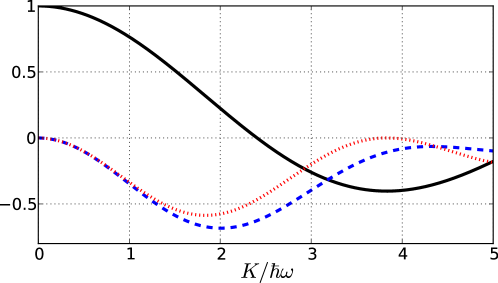
However, even though it is derived from a systematic expansion, this approximation is plagued by the following problem. For any finite order $\tilde{\nu}\geq 2$, the spectrum of the approximate Floquet Hamiltonian $\hat{H}^{FM[\tilde{\nu}]}_{t_{0}}$ possesses an artifactual dependence on $t_{0}$, or equivalently on the driving phase. This is not consistent with the spectrum of the exact Floquet Hamiltonian $\hat{H}_{t_{0}}^{F}$, which is independent of the driving phase. In second order, the $t_{0}$ dependence enters with the second term of Eq. (109). Let us consider, for example, a periodic Hamiltonian with even time dependence, $\hat{H}(t)=\hat{H}(-t)$, so that $\hat{H}_{m}=\hat{H}_{-m}$. In this case $\hat{H}^{F(2)}_{t_{0}}$ vanishes for $t_{0}$ being an integer multiple of $\pi/\omega$, while it is generally finite for other values of $t_{0}$. Therefore, generally the Floquet Hamiltonians $\hat{H}^{M[\tilde{\nu}]}_{Ft_{0}}$ and $\hat{H}^{M[\tilde{\nu}]}_{Ft_{0}^{\prime}}$ obtained from the Floquet-Magnus approximation for times $t_{0}\neq t_{0}^{\prime}$ are not related to each other by a unitary transformation, as it is the case for the exact Floquet Hamiltonian.

The origin of this spurious $t_{0}$ dependence lies in the fact that the expansion (104) of the Floquet Hamiltonian implies also an expansion $\hat{U}_{F}(t)=1+\hat{U}_{F}^{(1)}+\hat{U}_{F}^{(2)}(t)\cdots$ of the unitary operator $\hat{U}_{F}(t)$. At any finite order, such an expansion does not preserve unitarity and, thus, the spectrum of the approximate Floquet Hamiltonian $\hat{H}^{FM[\tilde{\nu}]}_{t_{0}}$ deviates from the $\tilde{\nu}$th-order spectrum obtained by diagonalizing the approximate effective Hamiltonian $\hat{H}_{F}^{[\tilde{\nu}]}$ given by Eq. (92).

This observation can be traced back further to the ansatz (103) for the time evolution operator. Bi-partitioning the time-evolution operator into two exponentials like in Eq. (103) does not allow for disentangling the phase evolution from the micromotion. This is different for the tri-partitioning ansatz

$$\hat{U}(t,t_{0}) = \hat{U}_{F}(t)\,\exp\bigg{(}-\frac{i}{\hbar}(t-t_{0})\hat{H}^{F}\bigg{)}\hat{U}_{F}^{\dagger}(t_{0})$$ (113)

$$= \exp\Big{(}\hat{G}(t)\Big{)}\,\exp\bigg{(}-\frac{i}{\hbar}(t-t_{0})\hat{H}^{F}\bigg{)}\exp\Big{(}-\hat{G}(t_{0})\Big{)},$$

which underlies the perturbative approach presented in the previous section. In the tri-partitioning ansatz (113), first $\hat{U}_{F}^{\dagger}(t_{0})$ transforms the state into a “reference frame” where by construction no micromotion is present. Then the phase evolution is generated by the effective Hamiltonian, before at time $t$ the state is finally rotated back to the original frame by $\hat{U}_{F}(t)$. In contrast $\hat{H}^{F}_{t_{0}}$, as it appears in the ansatz (103), carries also information about the micromotion. This fact is somewhat hidden, when the $t_{0}$ dependence of the Floquet Hamiltonian is not written out explicitly like in Ref. [47], where $t_{0}=0$ is assumed.

However, since we know that the effective Hamiltonian $\hat{H}_{F}$ and the Floquet Hamiltonian $\hat{H}^{F}_{t_{0}}$ possess the same spectrum, we also know that, when expanding both $\hat{H}_{F}$ and $\hat{H}^{F}_{t_{0}}$ in powers of the inverse frequency, also the spectra will coincide up to this order. This means that the $t_{0}$-dependent second term of Eq. (109) will not cause changes of the spectrum within the second order ($\propto\omega^{-1}$). Instead this second term can contribute to the third-order correction of the quasienergy spectrum, together with the terms of $\hat{H}_{t_{0}}^{(3)}$. This argument generalizes to higher orders.

Let us illustrate our reasoning using a simple example. A spin-1/2 system shall be described by the time-periodic Hamiltonian

$$\hat{H}(t)=a\hat{S_{x}}+b\cos(\omega t)\hat{S}_{y},$$ (114)

with spin operators $\hat{S}_{i}$ and Fourier components

$$\hat{H}_{0}=a\hat{S_{x}},\qquad\hat{H}_{1}=\hat{H}_{-1}=\frac{b}{2}\hat{S}_{y},\qquad\hat{H}_{m}=0\;\;\mathrm{for}\;\;|m|\geq 2.$$ (115)

According to equations (87) and (88), in second order the effective Hamiltonian is approximated by

$$\hat{H}_{F}\approx\hat{H}_{F}^{[2]}=\hat{H}_{F}^{(1)}+\hat{H}_{F}^{(2)},$$ (116)

with

$$\hat{H}_{F}^{(1)}=a\hat{S}_{x},\qquad\hat{H}_{F}^{(2)}=0.$$ (117)

Here the second-order term $\hat{H}_{F}^{(2)}$ vanishes since $[\hat{H}_{m},\hat{H}_{-m}]=0$. In second order the quasienergy spectrum is, thus, approximated by

$$\varepsilon_{\pm}\approx\varepsilon^{[2]}_{\pm}=\pm\frac{1}{2}\hbar a.$$ (118)

In contrast, the second-order approximation of the Floquet Hamiltonian based on the Floquet-Magnus expansion,

$$\hat{H}^{F}_{t_{0}}\approx\hat{H}_{t_{0}}^{FM[2]}=\hat{H}_{t_{0}}^{F(1)}+\hat{H}_{t_{0}}^{F(2)},$$ (119)

does contain a second-order term. Namely, from Eqs. (108) and (109) one obtains

$$\hat{H}_{t_{0}}^{F(1)}=a\hat{S}_{x},\qquad\hat{H}_{t_{0}}^{F(2)}=-\frac{ab}{\omega}\sin(\omega t_{0})\hat{S}_{z}.$$ (120)

It leads to the approximation of the quasienergy spectrum

$$\varepsilon_{\pm}\approx\varepsilon^{FM[2]}_{\pm} = \pm\frac{1}{2}\hbar a\sqrt{1+\big{[}(b/\omega)\sin(\omega t_{0})\big{]}^{2}}$$ (121)

$$= \pm\frac{1}{2}\hbar a\Big{(}1+\frac{1}{2}\big{[}(b/\omega)\sin(\omega t_{0})\big{]}^{2}+\cdots\Big{)}.$$

We can now make several observations that illustrate the reasoning of the previous paragraphs. First, we can see that $\varepsilon^{FM[2]}_{\pm}$ coincides with $\varepsilon^{[2]}_{\pm}$ within the order of the approximation. Deviations that occur are proportional to $\omega^{-2}$, while our second-order approximation should provide the correct terms up to the power $\omega^{-1}$. Second, despite the presence of a finite second-order term $\hat{H}_{t_{0}}^{F(2)}$ proportional to $\omega^{-1}$, $\varepsilon^{FM[2]}_{\pm}$ does not contain a correction $\propto\omega^{-1}$. This is consistent with the fact that $\hat{H}_{F}^{[2]}$ and, as a consequence, also $\varepsilon^{[2]}_{\pm}$ do not contain a second-order term. Third, we can see that, unlike the exact quasienergy spectrum, the approximate spectrum $\varepsilon^{FM[2]}_{\pm}$ depends on the time $t_{0}$ and, thus, also on the driving phase. However, this dependence on $t_{0}$ (or the driving phase) occurs only in terms $\propto\omega^{-2}$ that are not reproduced correctly within the second-order approximation. In a third-order approximation, the spectrum will be captured correctly and be independent of the driving phase up to the power $\omega^{-2}$ and so on.

As a further example, we will discuss the circularly driven hexagonal lattice in the next section. There, we will see that the spurious driving-phase dependence of the Floquet-Magnus expansion will, additionally, also induce a spurious breaking of the rotational symmetry of the quasienergy dispersion relation (Section 6.3). Thus, even a weak $t_{0}$ dependence can seemingly change the properties of the system in a fundamental way. Therefore, the Floquet-Magnus approximation should be used with care. The high-frequency approximation derived in the previous section 4 does not suffer from this problem.

6 Example: Circularly driven hexagonal lattice

In this section, we will discuss an instructive example of the physics of particles hopping on a hexagonal lattice [see Fig. 4(a)] subjected to a circular time-periodic force

$${\bm{F}}(t)=-F[\cos(\omega t){\bm{e}}_{x}+\sin(\omega t){\bm{e}}_{y}].$$ (122)

For a system of charged electrons such a force can be realized by applying circularly polarized light, whereas for a system of neutral particles (atoms in an optical lattice or photons in a wave guide) it can be achieved as an inertial force via circular lattice shaking [25, 26, 39, 38]. The driven hexagonal lattice is particularly interesting, as it is the prototype of a Floquet topological insulator [27, 57, 58, 59, 60]. It was pointed out by Oka and Aoki [27] that a non-vanishing forcing strength $F$ opens a topological gap in the band structure of the effective Hamiltonian. As a consequence, the system possesses a quantized Hall conductivity, when the lowest band is filled completely with fermions. While the original proposal [27] is considering graphene irradiated by circularly polarized light (see also Ref. [64]), the topologically non-trivial band structure described by the effective Hamiltonian has been probed experimentally in other systems: with classical light in a hexagonal lattice of wave guides [39] and with ultracold fermionic atoms in a circularly shaken optical lattice [38].

We have decided to discuss the circularly driven hexagonal lattice here, even though its single-particle physics has been described in detail already elsewhere [27, 58, 65, 38], because of several reasons. First, it is a paradigmatic example of a system where the second-order high-frequency correction to the effective Hamiltonian gives rise to qualitatively new physics. Second, since both directions, $x$ and $y$, are driven with a phase lag of $\pi/2$, the model is suitable to illustrate the difference between the high-frequency expansion advertised here and the Floquet-Magnus expansion. And third, it allows us to set the stage for the ensuing discussion (see Sect. 7) of the role of interactions, which have been discussed controversially recently [66, 67]. This issue includes two aspects: the impact of interactions on the validity of the high-frequency expansion as well as how interactions appear in the high-frequency expansion.

Figure 4: Hexagonal lattice with sublattice A (blue) and B (red). (a) The Hamiltonian $\hat{H}_{\mathrm{kin}}$ of the undriven model possesses real tunneling matrix elements $-J$ between neighboring sites. (b) The effective Hamiltonian $\hat{H}_{F}\approx\hat{H}_{F}^{(1)}+\hat{H}^{(2)}_{F}$ of the driven system features modified real tunneling matrix elements $-J^{(1)}$ between nearest neighbors, contained in $\hat{H}_{F}^{(1)}$, and complex tunneling matrix elements $-|J^{(2)}|e^{i\theta}$ (or $-|J^{(2)}|e^{-i\theta}$), contained in $\hat{H}_{F}^{(2)}$, for tunneling in anticlockwise (or clockwise) direction around the hexagonal plaquette.

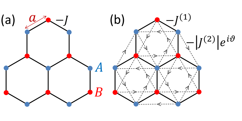
Let us consider the driven tight-binding Hamiltonian

$$\hat{H}_{\mathrm{dr}}(t)=-\sum_{\langle\ell^{\prime}\ell\rangle}J\hat{a}^{{\dagger}}_{\ell^{\prime}}\hat{a}^{\phantom{{\dagger}}}_{\ell}+\sum_{\ell}v_{\ell}(t)\hat{n}_{\ell}.$$ (123)

The first term describes the tunneling kinetics, with the sum running over all directed links $\langle\ell^{\prime}\ell\rangle$ connecting a site $\ell$ to its nearest neighbor $\ell^{\prime}$ on the hexagonal lattice depicted in Fig. 4(a). Here $\hat{a}^{\phantom{{\dagger}}}_{\ell}$ is the annihilation operator for a particle (boson or fermion) at the lattice site $\ell$ located at ${\bm{r}}_{\ell}$, and the tunneling parameter $J$ is real and positive. The second sum runs over the lattice sites and describes the effect of the driving force in terms of the time-periodic on-site potential $v_{\ell}(t)=-{\bm{r}}_{\ell}\cdot{\bm{F}}(t)$ and the number operator $\hat{n}_{\ell}=\hat{a}^{{\dagger}}_{\ell}\hat{a}^{\phantom{{\dagger}}}_{\ell}$. The direction of the vector pointing from site $\ell$ to a neighbor $\ell^{\prime}$ defines an angle $\varphi_{\ell^{\prime}\ell}$,

$${\bm{r}}_{\ell^{\prime}}-{\bm{r}}_{\ell}\equiv a[\cos(\varphi_{\ell^{\prime}\ell}){\bm{e}}_{x}+\sin(\varphi_{\ell^{\prime}\ell}){\bm{e}}_{y}],$$ (124)

with $\varphi_{\ell\ell^{\prime}}=\varphi_{\ell^{\prime}\ell}+\pi$. This angle determines the temporal driving phase of the relative potential modulation between both sites,

$$v_{\ell^{\prime}}(t)-v_{\ell}(t)=Fa\cos(\omega t-\varphi_{\ell^{\prime}\ell}).$$ (125)

6.1 Change of gauge

As will be seen shortly, we are interested in the regime of strong forcing, where the amplitude $K\equiv Fa$ of the relative potential modulation between two neighboring sites is comparable to or larger than $\hbar\omega$. Therefore, the Hamiltonian $\hat{H}_{\mathrm{dr}}(t)$ is not a suitable starting point for the high-frequency approximation.

A remedy is provided by a gauge transformation with the time-periodic unitary operator [25]

$$\hat{U}(t)=\exp\Big{(}i\sum_{\ell}\chi_{\ell}(t)\hat{n}_{\ell}\Big{)},$$ (126)

where

$$\chi_{\ell}(t) = -\int_{0}^{t}\!\mathrm{d}t^{\prime}\,\frac{v_{\ell}(t^{\prime})}{\hbar}+\frac{1}{T}\int_{0}^{T}\!\mathrm{d}t^{\prime\prime}\int_{0}^{t^{\prime\prime}}\!\mathrm{d}t^{\prime}\,\frac{v_{\ell}(t^{\prime})}{\hbar}$$ (127)

$$= \frac{F{\bm{r}}_{\ell}}{\hbar\omega}\cdot[-\sin(\omega t){\bm{e}}_{x}+\cos(\omega t){\bm{e}}_{y}].$$

This gauge transformation induces a time-dependent shift in quasimomentum, and the second integral has been included to eliminate an overall quasimomentum drift. It provides a constant that subtracts the zero-frequency component of the first integral, thus making the time average of $\chi_{\ell}(t)$ over one driving period vanish. One arrives at the translationally invariant time-periodic Hamiltonian

$$\hat{H}(t)=\hat{U}^{\dagger}(t)\hat{H}_{\mathrm{dr}}(t)\hat{U}(t)-{i\hbar\,}\hat{U}^{\dagger}(t)\dot{\hat{U}}(t)=-\sum_{\langle\ell^{\prime}\ell\rangle}Je^{i\theta_{\ell^{\prime}\ell}(t)}\hat{a}^{{\dagger}}_{\ell^{\prime}}\hat{a}^{\phantom{{\dagger}}}_{\ell}.$$ (128)

Here the scalar potential $v_{\ell}(t)$ is absent while the driving force is captured by the time-periodic Peierls phases

$$\theta_{\ell^{\prime}\ell}(t)=\chi_{\ell}(t)-\chi_{\ell^{\prime}}(t)=\frac{K}{\hbar\omega}\sin(\omega t-\varphi_{\ell^{\prime}\ell}).$$ (129)

Now we are in the position to apply the high-frequency approximation, even for $K\gg\hbar\omega$. The actual requirement is that $\hbar\omega$ must be large compared to the tunneling matrix element $J$, which determines both the spectral width of $\hat{H}_{0}$ and the strength of the coupling terms $\hat{H}_{m}$ with $m\neq 0$.

6.2 Effective Hamiltonian

The leading term in the expansion of the effective Hamiltonian is according to Eq. (87) given by the time-average of the driven Hamiltonian

$$\hat{H}_{F}^{(1)}=\hat{H}_{0}=-\sum_{\langle\ell^{\prime}\ell\rangle}J^{(1)}\hat{a}^{{\dagger}}_{\ell^{\prime}}\hat{a}^{\phantom{{\dagger}}}_{\ell}.$$ (130)

It corresponds to the undriven Hamiltonian with a modified effective tunneling matrix element

$$J^{(1)}=J\mathcal{J}_{0}\big{(}{\textstyle\frac{K}{\hbar\omega}}\big{)},$$ (131)

where $\mathcal{J}_{n}$ denotes a Bessel function of integer order $n$. This result was obtained by employing the relation

$$\exp(ir\sin(s))=\sum_{k=-\infty}^{\infty}\mathcal{J}_{k}(r)\exp(iks).$$ (132)

This Bessel-function-type renormalization of the tunnel matrix element, see Fig. 5 for a plot, allows to effectively reduce or even “switch off” completely the nearest neighbor tunneling matrix element. This effect is known as dynamic localization [3], coherent destruction of tunneling [4, 6], or band collapse [5]. It has been observed in the coherent expansion of a localized Bose condensate in a shaken optical lattice [7]. The effect has also been used to induce the transition between a bosonic superfluid to a Mott insulator (and back) by shaking an optical lattice [19, 20]. The possibility to make the tunneling matrix element negative has moreover been exploited to achieve kinetic frustration in a circularly forced triangular lattice and to mimic antiferromagnetism with spinless bosons [25, 26].

The second-order contribution to the effective Hamiltonian is given by Eq. (88) and can be written like

$$\hat{H}_{F}^{(2)}=\sum_{m=1}^{\infty}\frac{1}{m\hbar\omega}\big{[}\hat{H}_{m},\hat{H}_{-m}\big{]},$$ (133)

with the Fourier components of the Hamiltonian reading

$$\hat{H}_{m}=-\sum_{\langle\ell^{\prime}\ell\rangle}J\mathcal{J}_{m}\big{(}{\textstyle\frac{K}{\hbar\omega}}\big{)}e^{-im\varphi_{\ell^{\prime}\ell}}\,\hat{a}^{{\dagger}}_{\ell^{\prime}}\hat{a}^{\phantom{{\dagger}}}_{\ell}.$$ (134)

By using the relation $\big{[}\hat{a}^{{\dagger}}_{k}\hat{a}^{\phantom{{\dagger}}}_{l},\hat{a}^{{\dagger}}_{m}\hat{a}^{\phantom{{\dagger}}}_{n}\big{]}=\delta_{lm}\hat{a}^{{\dagger}}_{k}\hat{a}^{\phantom{{\dagger}}}_{n}-\delta_{kn}\hat{a}^{{\dagger}}_{m}\hat{a}^{\phantom{{\dagger}}}_{l}$, which holds both for bosonic and fermionic operators $\hat{a}^{\phantom{{\dagger}}}_{\ell}$, as well as $\mathcal{J}_{-m}(x)=(-)^{m}\mathcal{J}_{m}(x)$, one arrives at

$$\hat{H}^{(2)}_{F}=-\sum_{\langle\!\langle\ell^{\prime}\ell\rangle\!\rangle}J^{(2)}_{\mathrm{\langle\!\langle\ell^{\prime}\ell\rangle\!\rangle}}\,\hat{a}^{{\dagger}}_{\ell^{\prime}}\hat{a}^{\phantom{{\dagger}}}_{\ell},$$ (135)

where the sum runs over next-nearest neighbors $\ell^{\prime}$ and $\ell$. The effective tunneling matrix element is given by

$$J_{\langle\!\langle\ell^{\prime}\ell\rangle\!\rangle}^{(2)}=\frac{J^{2}}{\hbar\omega}\sum_{m=1}^{\infty}\frac{1}{m}\mathcal{J}_{m}^{2}\big{(}{\textstyle\frac{K}{\hbar\omega}}\big{)}2i\sin\big{(}m[\varphi_{\ell^{\prime}k}-\varphi_{\ell k}]\big{)},$$ (136)

where $k$ denotes the intermediate lattice site between $\ell^{\prime}$ and $\ell$, via which the second-order tunneling process occurs. One can immediately see that the tunneling matrix elements $J_{\langle\!\langle\ell^{\prime}\ell\rangle\!\rangle}^{(2)}$ are purely imaginary and that they depend, as an odd function, on the relative angle $\varphi_{\ell^{\prime}k}-\varphi_{\ell k}$ only. This relative angle is given by $\varphi_{\ell^{\prime}k}-\varphi_{\ell k}=-\sigma_{\ell^{\prime}\ell}\frac{2\pi}{3}$, with sign $\sigma_{\ell^{\prime}\ell}=+1$ ($\sigma_{\ell^{\prime}\ell}=-1$) for tunneling in anticlockwise (clockwise) direction around a hexagonal lattice plaquette. Therefore, one finds

$$J_{\langle\!\langle\ell^{\prime}\ell\rangle\!\rangle}^{(2)}=iJ^{(2)}\sigma_{\ell^{\prime}\ell}=|J^{(2)}|e^{i\sigma_{\ell^{\prime}\ell}\theta}$$ (137)

forming the pattern of effective tunneling matrix elements depicted in Fig. 4(b). Here

$$J^{(2)}=-\frac{J^{2}}{\hbar\omega}\sum_{m=1}^{\infty}\frac{1}{m}\mathcal{J}_{m}^{2}\big{(}{\textstyle\frac{K}{\hbar\omega}}\big{)}2\sin\big{(}m2\pi/3\big{)}\simeq-\sqrt{3}\frac{J^{2}}{\hbar\omega}\mathcal{J}_{1}^{2}\big{(}{\textstyle\frac{K}{\hbar\omega}}\big{)}$$ (138)

and

$$\theta=\mathrm{sign}(J^{(2)})\frac{\pi}{2}.$$ (139)

Since $|\mathcal{J}_{m}(x)|$ decays like $|x|^{|m|}$ with respect to the order $m$, for sufficiently small $K/\hbar\omega$ the sum is to good approximation exhausted by its first term, as is demonstrated also in Fig. 5.

Figure 5: Effective tunneling matrix elements $J^{(1)}/J$ (solid black line) and $J^{(2)}/(J^{2}/\hbar\omega)$ (dashed blue line), as well as the leading term $-\sqrt{3}\mathcal{J}_{1}^{2}(K/\hbar\omega)$ contributing to $J^{(2)}/(J^{2}/\hbar\omega)$ (dotted red line).

The approximate effective Hamiltonian [58]

$$\hat{H}_{F}\approx\hat{H}_{F}^{(1)}+\hat{H}_{F}^{(2)},$$ (140)

as it is depicted in Fig. 4(b), directly corresponds to the famous Haldane model [68] (see also reference [69]), being the prototype of a topological Chern insulator [70, 71]. The next-nearest neighbor tunneling matrix elements open a gap between the two low-energy Bloch bands of the hexagonal lattice, such that the bands acquire topologically non-trivial properties of a Landau level characterized by non-zero integer Chern number [72]. As a consequence, the system features chiral edge states, as they have been observed experimentally with optical wave guides [39], and a finite Hall conductivity, as it has been observed with ultracold fermionic atoms [38], which is quantized for a completely filled lower band. The fact that circular forcing can induce such non-trivial properties to a hexagonal lattice has been pointed out in Ref. [27]. This is the first proposal for a Floquet-topological insulator [60] (later proposals include Refs. [57, 59]). These systems can be defined as driven lattice systems with the effective Hamiltonian featuring new matrix elements that open topologically non-trivial gaps in the Floquet-Bloch band structure. Such new matrix elements appear in second (or higher) order of the high-frequency approximation that capture processes where a particle tunnels twice (or several times) during one driving period and that are of the order of $\sim J^{2}/\hbar\omega$. Therefore, Floquet topological insulators require the driving frequency to be at most moderately larger than the tunneling matrix element $J$. This is different for another class of schemes for the creation of artificial gauge fields and topological insulators recently pushed forward mainly in the context of ultracold quantum gases [30, 28, 29, 31, 32, 34, 35, 36, 37]. In these schemes non-trivial effects enter already in the leading first-order term of the high-frequency expansion, such that they work also in the high-frequency limit $\hbar\omega\gg J$.

The non-interacting driven hexagonal lattice considered in this section can easily be solved numerically, without further approximation. The driven Hamiltonian (128) obeys discrete translational lattice, with two sublattice states per lattice cell. As a consequence, the single-particle state space is divided into uncoupled sectors of sharp quasimomentum, each containing two states. The problem is reduced to that of a family of driven two-level systems labeled by the quasimomentum wave vector ${\bm{k}}$. The high-frequency approximation (140) is nevertheless useful. First, it gives rise to an analytical approximation to the Floquet Hamiltonian, directly corresponding to the paradigmatic Haldane model [58, 38]. Second, as we will argue in the next paragraph, the second-order approximation captures already the essential physics of the non-interacting system in the regime of large frequencies. And third, it allows for taking into account also some of the effects related to interactions (see section 7.1).

Let us briefly argue why the approximate effective Hamiltonian (140) captures the essential properties of the full one for the translationally invariant non-interacting system in the limit of large driving frequencies. The two-level Hamiltonian acting in the single-particle space of states with quasimomentum ${\bm{k}}$ is represented by a $2\times 2$ matrix of the general form $h({\bm{k}},t)=h_{0}({\bm{k}},t)+\bm{h}({\bm{k}},t)\cdot{\bm{\sigma}}$, with ${\bm{\sigma}}$ denoting the vector of Pauli matrices and vector $\bm{h}=(h_{x},h_{y},h_{z})$. If the elements $h_{i}({\bm{k}},t)\sim J$ are small compared to $\hbar\omega$, the perturbation expansion can be expected to converge. It is then left to argue that corrections beyond the second-order approximation (140) do not lead to qualitatively new behavior. This can be done employing the arguments by Haldane [68] (see also reference [69]). In the subspace of quasimomentum ${\bm{k}}$, the effective Hamiltonian $\hat{H}_{F}$ is represented by a time-independent matrix

$$h_{F}({\bm{k}})=h_{F0}({\bm{k}})+\bm{h}_{F}({\bm{k}})\cdot{\bm{\sigma}}.$$ (141)

Its components determine the single-particle quasienergy dispersion relation

$$\varepsilon^{F}_{\pm}({\bm{k}})=h_{F0}({\bm{k}})\pm\sqrt{|{\bm{h}}_{F}({\bm{k}})|},$$ (142)

with the two bands labeled by $-$ and $+$. The leading approximation of the effective Hamiltonian, $\hat{H}^{(1)}_{F}$, describes a hexagonal lattice with real nearest-neighbor tunneling matrix element $-J^{(1)}\sim J$ [see Fig. 4(b)]. It gives rise to a contribution ${\bm{h}}^{(1)}_{F}({\bm{k}})$ to the vector ${\bm{h}}_{F}({\bm{k}})$. Due to the fact that $\hat{H}^{(1)}_{F}$ obeys space-inversion and time-reversal symmetry, two inequivalent quasimomenta ${\bm{k}}_{\pm}$ (the corners $K$ and $K^{\prime}$ of the first Brillouin zone) exist, where ${\bm{h}}^{(1)}({\bm{k}}_{\pm})=0$ [69]. These are the Dirac points where the bands described by ${\bm{h}}^{(1)}({\bm{k}})$ touch in a cone-like fashion. Moreover, also $h_{z}^{(1)}({\bm{k}})=0$ for all ${\bm{k}}$, since nearest-neighbor tunneling contributes only to the sublattice-mixing off-diagonal matrix elements. Now, the second-order correction to the effective Hamiltonian $\hat{H}_{F}^{(2)}$ contains complex next-nearest-neighbor tunneling matrix elements $-|J^{(2)}|e^{\pm i\vartheta}$ [see Fig. 4(b)] of the order of $J^{2}/(\hbar\omega)$ [keeping $K/(\hbar\omega)$ fixed]. This gives rise to a correction ${\bm{h}}_{F}^{(2)}({\bm{k}})$, where only the $z$-component ${h}_{Fz}^{(2)}({\bm{k}})$ is non-zero, since next-nearest-neighbor tunneling is sublattice preserving. Moreover, the time-reversal symmetry breaking associated with the phase $\vartheta$ makes this $z$-component non-zero at the Dirac points, such that ${h}_{Fz}^{(2)}({\bm{k}}_{+})=-{h}^{(2)}_{Fz}({\bm{k}}_{-})\neq 0$. In this way the second-order correction removes the band touching and opens a gap between both bands. The opposite sign of ${h}^{(2)}_{Fz}({\bm{k}}_{+})$ and ${h}^{(2)}_{Fz}({\bm{k}}_{-})$ implies a finite Chern number of $\pm 1$ of the lowest band [68]. Now it is important to note that in second order the bands are separated by a gap of order $J^{2}/(\hbar\omega)$ (excluding situations, where the forcing strength is fine-tuned close to values giving $J^{(1)}=0$ or $J^{(2)}=0$). Even higher-order corrections, which in real space describe tunneling at even longer distances associated with a particle tunneling three or more times during one driving period, will be of the order of $J^{3}/(\hbar\omega)^{2}$. They will not be able to close this gap and change the topological properties of the bands anymore. Thus, the essential physics of the driven system is captured by the approximation (140).

Qualitatively new behavior beyond the high-frequency approximation occurs, however, when $\hbar\omega$ becomes small enough so that $\varepsilon^{F}_{+}({\bm{k}})-\varepsilon^{F}_{-}({\bm{k}})=m\hbar\omega$ with $m=1,2,3,\dots$ for some quasimomenta ${\bm{k}}$. In this case both bands are coupled resonantly in an $m$-“photon” process and hybridize. Such a hybridization is not captured by the perturbative approach underlying the high-frequency approximation. It occurs, roughly, when the gap between subspaces of different “photon” number closes. The new band gaps resulting from the avoided quasienergy level crossing between the states of quasienergy $\varepsilon^{F}_{-}({\bm{k}})$ and $\varepsilon^{F}_{+}({\bm{k}})-m\hbar\omega$ have been shown to give rise to intriguing topological properties without analog in non-driven systems [57, 73].

6.3 Comparison with Floquet-Magnus expansion

The circularly driven hexagonal lattice is also an instructive example that illustrates the difference between the high-frequency expansion of the effective Hamiltonian $\hat{H}_{F}$ on the one hand and of the Floquet Hamiltonian $\hat{H}_{t_{0}}^{F}$, as it appears in the Floquet-Magnus expansion, on the other.

According to Eqs. (108) and (109), the leading terms of the expansion of $\hat{H}^{F}_{t_{0}}$ read

$$\hat{H}^{F(1)}_{t_{0}}=\hat{H}^{(1)}_{F}$$ (143)

and

$$\hat{H}^{F(2)}_{t_{0}}=\hat{H}^{(2)}_{F}+\sum_{m\neq 0}\frac{1}{m\hbar\omega}e^{im\omega t_{0}}[\hat{H}_{0},\hat{H}_{m}].$$ (144)

Evaluating the difference between the Floquet Hamiltonian and the effective Hamiltonian in second order, one obtains

$$\hat{H}^{F(2)}_{t_{0}}-\hat{H}^{(2)}_{F}=-\sum_{\langle\!\langle\ell^{\prime}\ell\rangle\!\rangle}J^{(2)}_{t_{0}\langle\!\langle\ell^{\prime}\ell\rangle\!\rangle}\,\hat{a}^{{\dagger}}_{\ell^{\prime}}\hat{a}^{\phantom{{\dagger}}}_{\ell}.$$ (145)

Here

$$J^{(2)}_{t_{0}\langle\!\langle\ell^{\prime}\ell\rangle\!\rangle} = -\sum_{m\neq 0}\frac{J^{2}}{m\hbar\omega}\mathcal{J}_{0}\big{(}{\textstyle\frac{K}{\hbar\omega}}\big{)}\mathcal{J}_{m}\big{(}{\textstyle\frac{K}{\hbar\omega}}\big{)}\bigg{(}e^{im(\omega t_{0}-\varphi_{k\ell})}-e^{im(\omega t_{0}-\varphi_{\ell^{\prime}k})}\bigg{)}$$

$$\simeq -\frac{2J^{2}}{\hbar\omega}\mathcal{J}_{0}\big{(}{\textstyle\frac{K}{\hbar\omega}}\big{)}\mathcal{J}_{1}\big{(}{\textstyle\frac{K}{\hbar\omega}}\big{)}\big{[}\cos(\omega t_{0}-\varphi_{k\ell})-\cos(\omega t_{0}-\varphi_{\ell^{\prime}k})\big{]}$$

denotes the $t_{0}$-dependent part of the next-nearest-neighbor tunneling matrix element

$$J^{(2)}_{\langle\!\langle\ell^{\prime}\ell\rangle\!\rangle}+J^{(2)}_{t_{0}\langle\!\langle\ell^{\prime}\ell\rangle\!\rangle}$$ (147)

of $\hat{H}^{F(2)}_{t_{0}}$, with $k$ defined as the intermediate site between $\ell$ and $\ell^{\prime}$. It is easy to check that the tunneling matrix element (147) depends on the direction of tunneling and not only on whether a particle tunnels in clockwise or anticlockwise direction around a hexagonal plaquette. This directional dependence is determined by $t_{0}$ and does not only concern the phase, but also the amplitude of next-nearest-neighbor tunneling matrix element (147). The consequence is a spurious $t_{0}$-dependent breaking of the discrete rotational symmetry of the band structure of the approximate Floquet Hamiltonian $\hat{H}_{t_{0}}^{F(1)}+\hat{H}_{t_{0}}^{F(2)}$. This can be seen as follows.

Figure 6: Quasienergy dispersion relation $\varepsilon_{+}({\bm{k}})$ of the circularly driven hexagonal lattice, for $\hbar\omega/J=4$ and $K/(\hbar\omega)=1.2$. We compare the second-order high-frequency approximation of the effective Hamiltonian, $\varepsilon^{[2]}_{+}({\bm{k}})$, [(a) and blue line in (c)] with the second-order Floquet-Magnus approximation, $\varepsilon^{FM[2]}_{t_{0}+}({\bm{k}})$, evaluated for $\omega t_{0}=2\pi/3$ [(b) and red line in (c)]. The Floquet-Magnus approximation $\varepsilon^{FM[2]}_{t_{0}+}({\bm{k}})$ does not only acquire a spurious $t_{0}$ dependence, but also breaks the discrete rotational symmetry of the exact dispersion relation $\varepsilon_{+}({\bm{k}})$. In first order both approximations coincide, $\varepsilon^{FM[1]}_{t_{0}+}({\bm{k}})=\varepsilon^{[1]}_{+}({\bm{k}})$ [dashed line in (c)].

The driven Hamiltonian $\hat{H}(t)$ obeys the discrete translational symmetry of the hexagonal lattice so that quasimomentum is a conserved quantity. Therefore, $\hat{H}^{F}_{t_{0}}$ and $\hat{H}_{F}$ do not only possess the same spectrum, but also the same single-particle dispersion relation $\varepsilon_{\pm}({\bm{k}})$. The symmetry of the hexagonal lattice with respect to discrete spatial rotations by $2\pi/3$ is broken by the periodic force. However, the force leaves the Hamiltonian $\hat{H}(t)$ unaltered with respect to the joint operation of a rotation by $2\pi/3$ combined with a time shift by $-T/3$. This spatio-temporal symmetry ensures that the effective Hamiltonian $\hat{H}_{F}$ possesses again the full discrete rotational symmetry of the hexagonal lattice. This is reflected in the leading terms (130) and (135) of the high-frequency expansion. As a consequence, the quasienergy band structure, given by the single particle dispersion relation $\varepsilon_{\pm}({\bm{k}})$, is also symmetric with respect to a spatial rotation by $2\pi/3$. The Floquet Hamiltonian $\hat{H}_{t_{0}}^{F}$, whose parametric dependence on the time $t_{0}$ indicates that it depends also on the micromotion, does not obey the discrete rotational symmetry of the hexagonal lattice when evaluated for a fixed time $t_{0}$. However, the single-particle spectrum of $\hat{H}_{t_{0}}^{F}$ is still given by $\varepsilon_{\pm}({\bm{k}})$ and, thus, rotationally symmetric. This latter property of the exact Floquet Hamiltonian $\hat{H}^{F}_{t_{0}}$ is not preserved by the Floquet-Magnus approximation $\hat{H}^{FM[2]}_{t_{0}}=\hat{H}_{t_{0}}^{F(1)}+\hat{H}_{t_{0}}^{F(2)}$. Here the second-order term does not only lead to a spurious $t_{0}$ dependence of the spectrum, but also breaks the rotational symmetry of the quasienergy band structure. This is illustrated in Fig. 6, where we compare the approximate dispersion relation $\varepsilon^{[2]}_{+}({\bm{k}})$ resulting from the high-frequency approximation of the effective Hamiltonian with the spectrum $\varepsilon^{FM[2]}_{t_{0}+}({\bm{k}})$ obtained using the Floquet-Magnus approximation. In this respect, the approximate Floquet Hamiltonian $\hat{H}^{FM[2]}_{t_{0}}$ is inconsistent with Floquet theory. The origin of this inconsistency is that the dispersion relation in Floquet-Magnus approximation depends on the driving phase, which, in turn, depends on the direction. Even though the spurious symmetry breaking should be small and of the order of $J(J/\hbar\omega)^{2}$ [for $(K/\hbar\omega)$ fixed], corresponding to the neglected third order, it still changes the property of the system in a fundamental way. Therefore, the Floquet-Magnus expansion has to be employed with care.

6.4 Micromotion

The micromotion operator $\hat{U}_{F}(t)=\exp\big{(}\hat{G}(t)\big{)}$ resulting from the periodic Hamiltonian $\hat{H}(t)$ is approximated by $\hat{G}(t)\approx\hat{G}^{(0)}(t)+\hat{G}^{(1)}(t)$. Here $\hat{G}^{(0)}(t)=0$ and, employing Eq. (69), we find

$$\hat{G}^{(1)}(t)=-\sum_{m=1}^{\infty}\frac{e^{im\omega t}\hat{H}_{m}-e^{-im\omega t}\hat{H}_{-m}}{m\hbar\omega}=\sum_{\langle\ell^{\prime}\ell\rangle}g_{\ell^{\prime}\ell}(t)\hat{a}^{{\dagger}}_{\ell^{\prime}}\hat{a}^{\phantom{{\dagger}}}_{\ell}\;,$$ (148)

with

$$g_{\ell^{\prime}\ell}(t) = -\frac{J}{\hbar\omega}\sum_{m=1}^{\infty}\frac{1}{m}\mathcal{J}_{m}\big{(}{\textstyle\frac{K}{\hbar\omega}}\big{)}\Big{[}e^{im(\omega t-\varphi_{\ell^{\prime}\ell})}-(-)^{m}e^{-im(\omega t-\varphi_{\ell^{\prime}\ell})}\Big{]}$$ (149)

$$\simeq -\frac{2J}{\hbar\omega}\mathcal{J}_{1}\big{(}{\textstyle\frac{K}{\hbar\omega}}\big{)}\cos(\omega t-\varphi_{\ell^{\prime}\ell}).$$

Since $\varphi_{\ell\ell^{\prime}}=\varphi_{\ell^{\prime}\ell}+\pi$, it follows that $g_{\ell^{\prime}\ell}(t)=-g^{*}_{\ell\ell^{\prime}}(t)$, such that $\hat{G}^{(1)}(t)$ is anti-hermitian as required. With respect to the original frame of reference, where the system is described by the driven Hamiltonian $\hat{H}_{\mathrm{dr}}(t)$, the micromotion operator is given by

$$\hat{U}_{\mathrm{dr}}^{F}(t) = \hat{U}_{F}(t)\hat{U}(t)\approx\exp\Bigg{(}\sum_{\langle\ell^{\prime}\ell\rangle}g_{\ell^{\prime}\ell}(t)\hat{a}^{{\dagger}}_{\ell^{\prime}}\hat{a}^{\phantom{{\dagger}}}_{\ell}\Bigg{)}\exp\Bigg{(}i\sum_{\ell}\chi_{\ell}(t)\hat{n}_{\ell}\Bigg{)}.$$

The dynamics that is described by $\hat{U}(t)$ does not happen in real space, but corresponds to a global time-periodic oscillation in quasimomentum by $\frac{K}{\hbar\omega}\frac{\hbar}{a}[\sin(\omega t){\bm{e}}_{x}-\cos(\omega t){\bm{e}}_{y}]$. This momentum oscillation is significant when $K\sim\hbar\omega$ and it is taken into account via the initial gauge transformation in a non-perturbative fashion, as can be seen from the Bessel-function-type dependence of the effective tunneling matrix elements on $K/\hbar\omega$. In turn, $\hat{U}_{F}(t)$ conserves quasimomentum and describes a micromotion in real space. This real-space micromotion becomes significant, when the tunneling time $2\pi\hbar/J$ is not too large compared to the driving period $T$, i.e. for $J/\hbar\omega$ not too small. A significant second-order correction $\hat{H}_{F}^{(2)}$ is a direct consequence of this real-space micromotion. In the high-frequency expansion, the real-space micromotion is taken into account perturbatively.

By expanding the tunneling matrix elements also in powers of the driving strength $K$, one finds that

$$\frac{J^{(2)}}{J^{(1)}}\simeq-\sqrt{3}\frac{JK^{2}}{(\hbar\omega)^{3}}.$$ (151)

The quadratic dependence on $K$ indicates that large driving amplitudes $K/\hbar\omega\sim 1$ are important in order to achieve a topological band gap $\sim|J^{(2)}|$ that is significant with respect to the band width $\sim|J^{(1)}|$. At the same time, the linear dependence on the tunneling matrix element $J$ reveals that moderate values of $J/\hbar\omega$, for which the high-frequency expansion is still justified, can be sufficient (see also Fig. 5).

The time-dependent basis states capturing the micromotion can be constructed from the basis of Fock states $|\{n_{\ell}\}\rangle$ characterized by sharp on-site occupation numbers $n_{\ell}$. They read

$$|\{n_{\ell}\}(t)\rangle_{F} = \hat{U}_{F}(t)|\{n_{\ell}\}\rangle\approx\exp\Bigg{(}\sum_{\langle\ell^{\prime}\ell\rangle}g_{\ell^{\prime}\ell}(t)\hat{a}^{{\dagger}}_{\ell^{\prime}}\hat{a}^{\phantom{{\dagger}}}_{\ell}\Bigg{)}|\{n_{\ell}\}\rangle$$ (152)

$$\approx \bigg{(}1-\sum_{\langle\ell^{\prime}\ell\rangle}\frac{2J}{\hbar\omega}\mathcal{J}_{1}\big{(}{\textstyle\frac{K}{\hbar\omega}}\big{)}\cos(\omega t-\varphi_{\ell^{\prime}\ell})\hat{a}^{{\dagger}}_{\ell^{\prime}}\hat{a}^{\phantom{{\dagger}}}_{\ell}\bigg{)}|\{n_{\ell}\}\rangle,$$

For the second approximation we have expanded the exponential, such that the state is normalized only up to terms of order $|J/\hbar\omega|^{2}$, and replaced $g_{\ell^{\prime}\ell}(t)$ by the leading term of the sum (149). The micromotion is dominated by the oscillatory dynamics of particles from one lattice site to a neighboring one and back. The probability for a particle participating in such an oscillation is of the order of $\big{|}\frac{2zJ}{\hbar\omega}\mathcal{J}_{1}\Big{(}\frac{K}{\hbar\omega}\Big{)}\big{|}^{2}$, with the coordination number $z=3$ counting the nearest neighbors of a lattice site.

7 Role of interactions

If we consider a periodically driven quantum system of many particles, then the presence of interactions will influence the high-frequency expansion in two different ways. First, the interaction terms in the Hamiltonian will simply generate new terms in the high-frequency expansion. This effect will be discussed in the following subsection 7.1 for the example of the driven tight-binding lattice discussed in the previous section. Second, the presence of interactions will severely challenge the validity of the high-frequency expansion, since even if the single-particle spectrum is bounded with a width lower than $\hbar\omega$, this will not be the case anymore for collective excitations. This issue will be addressed in subsection 7.2.

7.1 Interaction corrections within the high-frequency expansion

Ignoring for the moment concerns that the high-frequency expansion should be employed with care in the presence of interactions, let us have a look at the new terms that will be generated by finite interaction terms in the Hamiltonian. We will focus on the example of the driven tight-binding lattice that was discussed on the single-particle level in the previous section.

Starting from the interacting problem $\hat{H}_{\mathrm{dr}}(t)+\hat{H}_{\mathrm{int}}$ with a time-independent interaction term $\hat{H}_{\mathrm{int}}$ of the typical density-density type, the interactions are not altered by the gauge transformation (128). Thus, after the gauge transformation the interacting lattice system is described by the driven Hubbard Hamiltonian

$$\hat{H}(t)+\hat{H}_{\mathrm{int}},$$ (153)

with the time-periodic single-particle Hamiltonian $\hat{H}(t)$ given by Eq. (128). The presence of the time-independent term $\hat{H}_{\mathrm{int}}$, with trivial Fourier components

$$\hat{H}_{\mathrm{int}\,m}=\delta_{m,0}\hat{H}_{\mathrm{int}},$$ (154)

will lead to additional terms in the high-frequency expansion of the effective Hamiltonian that we will denote by $\hat{H}^{(m)}_{F\mathrm{int}}$. The leading contribution appears in the first order [Eq. (87)] and is given by the time-independent operator $\hat{H}_{\mathrm{int}}$ itself,

$$\hat{H}^{(1)}_{F\mathrm{int}}=\hat{H}_{\mathrm{int}}.$$ (155)

The second-order correction (88) vanishes,

$$\hat{H}^{(2)}_{F\mathrm{int}}=0,$$ (156)

because all Fourier components $\hat{H}_{\mathrm{int}\,m}$ with $|m|>0$ vanish. Therefore, the leading correction involving the interactions appears in third order [Eq. (4.2)] and reads

$$\hat{H}^{(3)}_{F\mathrm{int}}=\sum_{m=1}^{\infty}\Bigg{(}\frac{\big{[}\hat{H}_{-m},[\hat{H}_{\mathrm{int}},\hat{H}_{m}]\big{]}}{2(m\hbar\omega)^{2}}+\mathrm{h.c.}\Bigg{)}.$$ (157)

Here $\hat{H}_{m}$ denotes a Fourier component of the kinetic part $\hat{H}(t)$ of the Hamiltonian given by Eq. (134) of the previous section and “h.c.” stands for “hermitian conjugate”. The presence of interaction corrections beyond the leading order $\hat{H}^{(1)}_{F\mathrm{int}}=\hat{H}_{\mathrm{int}}$, as they result from real-space micromotion, was overlooked in a recent work investigating the possibility of stabilizing a fractional-Chern-insulator-type many-body Floquet state with interacting fermions in the circularly driven hexagonal lattice [66]. A recent study, which is based on the results presented here, investigates the impact of the correction (157) on the stability of both fermionic and bosonic Floquet fractional Chern insulators [74]. It is found that the correction tends to destabilize such a topologically ordered phase.

Note that the high-frequency expansion of the Floquet Hamiltonian $\hat{H}^{F}_{t_{0}}$, as it appears in the Floquet-Magnus expansion, produces also a second-order correction (109) that involves the interactions. It is given by [49, 48, 67]

$$\hat{H}^{F(2)}_{\mathrm{int},t_{0}}=\sum_{m=1}^{\infty}\frac{1}{m\hbar\omega}e^{im\omega t_{0}}[\hat{H}_{\mathrm{int}},\hat{H}_{m}].$$ (158)

However, as we have discussed in section 5, if we approximate the Floquet Hamiltonian in second order this term will not influence the many-body spectrum within the order of the approximation, while it introduces an unphysical dependence of the spectrum on the driving phase.

In order to get an idea of what type of terms appear in the high-frequency expansion, let us write down the third-order interaction correction for the simple case of spinless bosons in the circularly forced hexagonal lattice with on-site interactions

$$\hat{H}_{\mathrm{int}}=\frac{U}{2}\sum_{\ell}\hat{n}_{\ell}(\hat{n}_{\ell}-1).$$ (159)

This model system provides a quantitative description of ultracold bosonic atoms in an optical lattice and is interesting also because it might (as well as the fermionic system [66]) be a possible candidate for a system stabilizing a Floquet fractional Chern insulator state. Using Eq. (157), we find those third-order correction terms that involve the interactions to be given by

$$\hat{H}^{(3)}_{F\mathrm{int}} = -\sum_{\ell}2zW_{a}^{(3)}\hat{n}_{\ell}(\hat{n}_{\ell}-1)$$ (160)

$$+\,\sum_{\langle\ell^{\prime}\ell\rangle}\Big{\{}4W_{a}^{(3)}\hat{n}_{\ell^{\prime}}\hat{n}_{\ell}+2W_{b}^{(3)}\hat{a}^{{\dagger}}_{\ell^{\prime}}\hat{a}^{{\dagger}}_{\ell^{\prime}}\hat{a}^{\phantom{{\dagger}}}_{\ell}\hat{a}^{\phantom{{\dagger}}}_{\ell}\Big{\}}$$

$$+\,\sum_{\langle\ell^{\prime}k\ell\rangle}\Big{\{}W^{(3)}_{c}\hat{a}^{{\dagger}}_{\ell^{\prime}}\big{(}4\hat{n}_{k}-\hat{n}_{\ell}-\hat{n}_{\ell^{\prime}}\big{)}\hat{a}^{\phantom{{\dagger}}}_{\ell}$$

$$\qquad+\,W^{(3)}_{d}\big{(}\hat{a}^{{\dagger}}_{k}\hat{a}^{{\dagger}}_{k}\hat{a}^{\phantom{{\dagger}}}_{\ell^{\prime}}\hat{a}^{\phantom{{\dagger}}}_{\ell}+\hat{a}^{{\dagger}}_{\ell}\hat{a}^{{\dagger}}_{\ell^{\prime}}\hat{a}^{\phantom{{\dagger}}}_{k}\hat{a}^{\phantom{{\dagger}}}_{k}\big{)}\Big{\}}\bigg{]},$$

with coordination number $z=3$ and coupling strengths

$$W_{a}^{(3)} = \frac{UJ^{2}}{(\hbar\omega)^{2}}\sum_{m=1}^{\infty}\frac{1}{m^{2}}\mathcal{J}_{m}^{2}\big{(}{\textstyle\frac{K}{\hbar\omega}}\big{)}\simeq\frac{UJ^{2}}{(\hbar\omega)^{2}}\mathcal{J}_{1}^{2}\big{(}{\textstyle\frac{K}{\hbar\omega}}\big{)},$$ (161)

$$W_{b}^{(3)} = \frac{UJ^{2}}{(\hbar\omega)^{2}}\sum_{m=1}^{\infty}\frac{(-)^{m+1}}{m^{2}}\mathcal{J}_{m}^{2}\big{(}{\textstyle\frac{K}{\hbar\omega}}\big{)}\simeq\frac{UJ^{2}}{(\hbar\omega)^{2}}\mathcal{J}_{1}^{2}\big{(}{\textstyle\frac{K}{\hbar\omega}}\big{)},$$ (162)

$$W^{(3)}_{c} = \frac{UJ^{2}}{(\hbar\omega)^{2}}\sum_{m=1}^{\infty}\frac{1}{m^{2}}\cos\left(\frac{2\pi m}{3}\right)\mathcal{J}_{m}^{2}\big{(}{\textstyle\frac{K}{\hbar\omega}}\big{)}\simeq-\frac{UJ^{2}}{2(\hbar\omega)^{2}}\mathcal{J}_{1}^{2}\big{(}{\textstyle\frac{K}{\hbar\omega}}\big{)},$$ (163)

$$W^{(3)}_{d} = \frac{UJ^{2}}{(\hbar\omega)^{2}}\sum_{m=1}^{\infty}\frac{(-)^{m+1}}{m^{2}}\cos\left(\frac{2\pi m}{3}\right)\mathcal{J}_{m}^{2}\big{(}{\textstyle\frac{K}{\hbar\omega}}\big{)}\simeq-\frac{UJ^{2}}{2(\hbar\omega)^{2}}\mathcal{J}_{1}^{2}\big{(}{\textstyle\frac{K}{\hbar\omega}}\big{)}.$$

The third sum runs over all directed three-site strings $\langle\ell^{\prime}k\ell\rangle$, defined such that $\ell$ and $k$ as well as $k$ and $\ell^{\prime}$ are nearest neighbors, while $\ell\neq\ell^{\prime}$. The first sum produces a correction that reduces the on-site interactions of the leading term $\hat{H}^{(1)}_{F\mathrm{int}}=\hat{H}_{\mathrm{int}}$. The second sum introduces both nearest-neighbor density-density interactions like in the extended Hubbard model and a pair-tunneling term. And the third sum, finally describes density-assisted tunneling between next-nearest neighbors, as well as the joint tunneling of two-particles into or away from a given site.

7.2 On the validity of the high-frequency approximation for many-body systems

The high-frequency expansion of the effective Hamiltonian $\hat{H}_{F}$ and the micromotion operator $\hat{U}_{F}(t)$ can generally not be expected to converge for a system of many interacting particles. Namely, the time average $\hat{H}_{0}$ of the full many-body Hamiltonian $\hat{H}(t)$, which determines the spectrum of the diagonal blocks of the quasienergy operator $\bar{Q}$ depicted in Fig. 1, will possess collective excitations also at very large energies. Therefore the energy gaps of $\hbar\omega$, which separate the subspaces of different “photon” numbers $m$ in the unperturbed problem $\bar{Q}_{0}$, will close when the perturbation is switched on (unless $\hbar\omega$ was a macroscopic energy).

Figure 7: Like Fig. 3, but with the spectral width defined by $\varepsilon^{(0)}_{\alpha}$ larger than the energetic separation $\hbar\omega$ of sectors with different “photon” number $m$. The perturbation expansion is not justified and cannot be expected to converge. However, defining the unperturbed problem like in subfigure (b), the perturbation expansion can still be written down formally and, under certain conditions, still provide a useful approximation.

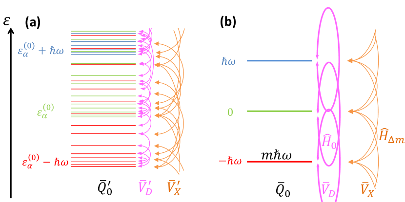
Nevertheless, the fact that the unperturbed problem $\bar{Q}_{0}$ is given by the “photonic” part of the quasienergy operator, with exactly degenerate eigenvalues $m\hbar\omega$ in each subspace of photon number $m$, allows one to formally write down the perturbation expansion. The energy denominators will not diverge. This is illustrated in Fig. 7. And, even if the perturbation expansion can generally not be expected to converge, these terms can still provide an approximate description of the driven many-body system on a finite time scale. This can be the case if the $\nu$th-order approximate effective Hamiltonian $\hat{H}_{F}^{[\nu]}$ is governed by energy scales that are small compared to $\hbar\omega$. Then the creation of a collective excitation of energy $\hbar\omega$ corresponds to a significant change in the structure of the many-body wave function and is a process associated with a very small matrix element only. As a consequence, on time scales that are small compared to the inverse of such residual matrix elements, the approximate effective Hamiltonian can be employed to compute the dynamics and approximate Floquet states of the system. This is the basis for Floquet engineering in interacting systems.

Let us illustrate this rather abstract reasoning by a concrete example. Consider again spinless bosons in the circularly forced hexagonal lattice, described by the driven Bose-Hubbard Hamiltonian (153). The first-order approximation to the effective Hamiltonian is given by

$$\hat{H}_{F}^{(1)}=-J\mathcal{J}_{0}\big{(}{\textstyle\frac{K}{\hbar\omega}}\big{)}\sum_{\langle\ell^{\prime}\ell\rangle}\hat{a}^{{\dagger}}_{\ell^{\prime}}\hat{a}^{\phantom{{\dagger}}}_{\ell}+\frac{U}{2}\sum_{\ell}\hat{n}_{\ell}(\hat{n}_{\ell}-1).$$ (165)

In the thermodynamic limit (where the number of lattice sites $M$ is taken to infinity, while keeping the filling of $n$ particles per lattice site fixed) the system possesses excited states at arbitrarily large energies. Therefore, the width of the spectrum is obviously larger than $\hbar\omega$. As a consequence, the first-order quasienergy spectrum that describes the subspace of “photon” number $m$ is much wider than $\hbar\omega$. It is not separated by a spectral gap from subspaces of different “photon number” anymore, but overlaps with quasienergies from these spectra. Therefore, the perturbation expansion, which is based on the assumption that the unperturbed spectral gaps do not close in response to the perturbation, can generally not be expected to converge. Namely, if we would consider the full diagonal blocks of the quasienergy matrix (Fig. 1) as unperturbed problem, that is if we would add the block-diagonal part of the supposedly perturbation to the unperturbed quasienergy operator considered before, already the unperturbed quasienergy spectra of different subspaces $m$ would overlap. As a consequence the energy denominators appearing in the perturbation expansion would diverge, whenever a degeneracy between unperturbed states of different “photon” number $m$ occurs.

We can now identify processes that spoil the high-frequency expansion for the driven Bose-Hubbard model (153) and estimate the time scale on which they occur. For simplicity, we focus on the limit of strong interactions $U\gg J$ and assume a filling of $n=1$. In the spirit of the argument presented at the end of the preceding paragraph, we can now add part of the perturbation to the unperturbed problem. We include the interactions in the definition of the unperturbed quasienergy operator,

$$\hat{Q}^{\prime}_{0}=\hat{H}_{\mathrm{int}}-i\hbar\mathrm{d}_{t},$$ (166)

so that the perturbation is given by the kinetic part (128) of the Hamiltonian,

$$\hat{V}^{\prime}(t)=\hat{H}(t)=\sum_{m}\hat{H}_{m}e^{im\omega t},$$ (167)

with Fourier components $\hat{H}_{m}$ given by Eq. (134). The unperturbed Floquet states $|\{n_{\ell}\}m\rangle\!\rangle$ are characterized by sharp site occupation numbers $n_{\ell}$ as well as sharp “photon” numbers $m$ and read

$$|\{n_{\ell}\}m(t)\rangle=e^{im\omega t}|\{n_{\ell}\}\rangle.$$ (168)

They diagonalize the unperturbed problem,

$$\langle\!\langle\{n^{\prime}_{\ell}\}m^{\prime}|\hat{Q}^{\prime}_{0}|\{n_{\ell}\}m\rangle\!\rangle=\delta_{m^{\prime},m}\delta_{\{n^{\prime}_{\ell}\},\{n_{\ell}\}}\varepsilon^{\prime(0)}_{\{n_{\ell}\}m},$$ (169)

where the unperturbed quasienergies read

$$\varepsilon^{\prime(0)}_{\{n_{\ell}\}m}=\frac{U}{2}\sum_{\ell}n_{\ell}(n_{\ell}-1)+m\hbar\omega.$$ (170)

The high-frequency approximation is spoiled whenever two unperturbed states $|\{n_{\ell}\}m\rangle\!\rangle$ and $|\{n^{\prime}_{\ell}\}m^{\prime}\rangle\!\rangle$ with different photon numbers $m\neq m^{\prime}$ are nearly degenerate and coupled to each other (either directly or in a higher-order process). In such a situation a strong hybridization between these states of different “photon” number occurs, rather than a perturbative admixture of one state to the other as required by the high-frequency approximation.

Let us investigate in how far the unperturbed “ground state” of the $m=0$ manifold, $|\psi_{0}\rangle\!\rangle$, suffers from such detrimental coupling. This state corresponds to a Mott-insulator with one particle per site,

$$|\psi_{0}\rangle\!\rangle=|\{n_{\ell}=1\}0\rangle\!\rangle.$$ (171)

It is the only unperturbed $m=0$ state without any doubly occupied site, so that the interaction energy vanishes. Its quasienergy reads $\varepsilon^{\prime(0)}_{0}=0$. It is the approximate ground state of the approximate effective Hamiltonians (165) in the regime $U\gg J$ [75]. We can now systematically study the most relevant processes that couple $|\psi_{0}\rangle\!\rangle$ to states of “photon” number $m\neq 0$. For that purpose, we will follow the procedure applied to a one-dimensional chain in reference [51].

The state $|\psi_{0}\rangle\!\rangle$ is coupled directly (in first-order) to unperturbed states

$$|\langle\ell_{2}\ell_{1}\rangle m\rangle\!\rangle\equiv\frac{1}{\sqrt{2}}\hat{b}^{{\dagger}}_{\ell_{2}}\hat{b}^{\phantom{{\dagger}}}_{\ell_{1}}|\{n_{\ell}=1\}m\rangle\!\rangle,$$ (172)

with one particle-hole excitation on neighboring sites $\ell_{1}$ and $\ell_{2}$, $m$ photons, and unperturbed quasienergy $\varepsilon^{(0)}_{\langle\ell_{2}\ell_{1}\rangle m}=U+m\hbar\omega$. The resonance condition $\varepsilon^{(0)}_{\langle\ell_{2}\ell_{1}\rangle m}=\varepsilon^{\prime(0)}_{0}$ is fulfilled for frequencies

$$\hbar\omega=-\frac{U}{m}\qquad\mathrm{with}\qquad m=-1,-2,-3,\ldots.$$ (173)

They are labeled by the negative change of the “photon” number, $m$, associated with the transition $|\psi_{0}\rangle\!\rangle\to|\langle\ell_{2}\ell_{1}\rangle m\rangle\!\rangle$. The corresponding coupling matrix elements is of the order of $J$ and reads

$$C^{(1)}_{m}=\langle\!\langle\langle\ell_{2}\ell_{1}\rangle m|\bar{V}^{\prime}|\psi_{0}\rangle\!\rangle = \frac{1}{\sqrt{2}}\langle\{n_{\ell}=1\}|\hat{b}^{{\dagger}}_{\ell_{1}}\hat{b}^{\phantom{{\dagger}}}_{\ell_{2}}\hat{H}_{m}|\{n_{\ell}=1\}\rangle$$ (174)

$$= -\sqrt{2}J\mathcal{J}_{m}\big{(}{\textstyle\frac{K}{\hbar\omega}}\big{)}e^{im\varphi_{\ell_{2}\ell_{1}}}.$$

The time scale for the resonant creation of a particle-hole excitations in the effective ground state can thus be estimated to be given by $2\pi\hbar/C^{(1)}_{m}$. If $\hbar\omega$ is larger than $U$, the direct excitation of particle-hole pairs is not resonant, so that this type of heating process cannot spoil the high-frequency approximation.

The next-strongest type of process is the creation of a collective excitation consiting of two coupled (i.e. overlapping) particle-hole pairs, with two extra particles on a site $\ell_{3}$ and no particles on two neighboring sites $\ell_{1}$ and $\ell_{2}$. Such a state is given by

$$|(\langle\ell_{3}\ell_{1}\rangle\langle\ell^{\prime}\ell_{2}\rangle)m\rangle\!\rangle=\frac{1}{\sqrt{6}}\hat{b}^{{\dagger}}_{\ell_{3}}\hat{b}^{{\dagger}}_{\ell_{3}}\hat{b}^{\phantom{{\dagger}}}_{\ell_{1}}\hat{b}^{\phantom{{\dagger}}}_{\ell_{2}}|\{n_{\ell}=1\}m\rangle\!\rangle$$ (175)

and possesses the unperturbed quasienergy $\varepsilon^{(0)}_{(\langle\ell_{3}\ell_{1}\rangle\langle\ell_{3}\ell_{2}\rangle)m}=3U+m\hbar\omega$. The resonance condition $\varepsilon^{(0)}_{(\langle\ell_{3}\ell_{1}\rangle\langle\ell_{3}\ell_{2}\rangle)m}=\varepsilon^{\prime(0)}_{0}$ is fulfilled for frequencies

$$\hbar\omega=-\frac{3U}{m}\qquad\mathrm{with}\qquad m=-1,-2,-4,-5,-7\ldots.$$ (176)

Here we have omitted those $m$, for which already a dominating first-order resonance (173) occurs. The state (175) is coupled to $|\psi_{0}\rangle\!\rangle$ only indirectly, in a second-order process via intermediate states $|\langle\ell_{3}\ell_{1,2}\rangle m^{\prime}\rangle\!\rangle$ characterized a single particle-hole pair and photon number $m^{\prime}$. The coupling matrix element can be evalutated using degenerate perturbation theory and reads

$$C^{(2)}_{m} = \sum_{m^{\prime}=-\infty}^{\infty}\langle\!\langle(\langle\ell_{3}\ell_{1}\rangle\langle\ell_{3}\ell_{2}\rangle)m|\bar{V}\bigg{(}\sum_{\ell=\ell_{1},\ell_{2}}|\langle\ell_{3}\ell\rangle m^{\prime}\rangle\!\rangle\langle\!\langle\langle\ell_{3}\ell\rangle m^{\prime}|\bigg{)}\bar{V}|\psi_{0}\rangle\!\rangle$$ (177)

$$\times\frac{1}{2}\Bigg{[}\frac{1}{\varepsilon^{(0)}_{(\langle\ell_{3}\ell_{1}\rangle\langle\ell_{3}\ell_{2}\rangle)m}-\varepsilon^{(0)}_{\langle\ell_{3}\ell_{1,2}\rangle m^{\prime}}}+\frac{1}{\varepsilon^{(0)}_{0}-\varepsilon^{(0)}_{\langle\ell_{3}\ell_{1,2}\rangle m^{\prime}}}\Bigg{]}$$

$$= \frac{\sqrt{6}J^{2}}{\hbar\omega}\sum_{m^{\prime}}\frac{\mathcal{J}_{m-m^{\prime}}\big{(}{\textstyle\frac{K}{\hbar\omega}}\big{)}\mathcal{J}_{m^{\prime}}\big{(}{\textstyle\frac{K}{\hbar\omega}}\big{)}}{m/3-m^{\prime}}$$

$$\times\bigg{(}e^{i(m-m^{\prime})\varphi_{\ell_{3}\ell_{2}}+im^{\prime}\varphi_{\ell_{3}\ell_{1}}}+e^{i(m-m^{\prime})\varphi_{\ell_{3}\ell_{1}}+im^{\prime}\varphi_{\ell_{3}\ell_{2}}}\bigg{)}.$$

In order to arrive at a simple result, we have focused on the vicinity of the resonance and employed $U=-m\hbar\omega/3$ in the energy denominators. The time scale for the resonant creation of such an overlapping pair of particle-hole excitations is given by $2\pi\hbar/C^{(2)}_{m}$. It is increased by a factor of the order of $\hbar\omega/J$ with respect to the creation of a single particle-hole pair, since it appears one order higher in perturbation theory. The experimentalists can avoid heating processes associated with the creation of two coupled particle-hole excitations by choosing $\hbar\omega$ well above $3U$. In this case, the most detrimental process will be the creation of a collective excitation given by three overlapping particle-hole pairs in a third-order process, with matrix element $C^{(3)}_{m}\sim J^{3}/(\hbar\omega)^{2}$. These third-order heating processes can, in turn, be avoided for $\hbar\omega$ well above $12U$, and so on. Thus, by increasing the driving frequency, the time scale for detrimental heating due to the creation of collective excitations increases.

The order of perturbation theory in which detrimental heating processes beyond the high-frequency approximation occur increases like a power law with the frequency $\hbar\omega$, at least for the model and the parameters considered. This suggests that the time scale for heating due to the creation of collective excitations increases exponentially with the driving frequency (the higher the energy of a collective excitation the more complex it is and the smaller will be the matrix element for its creation). Such a scaling is favorable for quantum engineering based on the high-frequency approximation. However, one has to note that the driving frequency cannot simply be increased to arbitrarily large values, because with increasing driving frequency another type of heating process will become more relevant. Namely, the resonant creation of high-energy single-particle states neglected in a low-energy model will become more and more relevant. In the driven lattice system these states belong to excited Bloch bands above a large energy gap $\Delta$ that are not taken into account in the tight binding description. If the resonance condition $\Delta\approx m\hbar\omega$ is fulfilled, these states can be populated in $m$-photon processes [76, 77, 78], the time scale of which tends to increase with $m$. Thus, Floquet engineering requires a window of suitable driving frequencies that are both large enough to suppress heating due to the creation of collective excitations and small enough to suppress heating due to interband transitions. In optical lattice systems, the existence of a window of suitable driving frequencies has been demonstrated in a number of experiments (see first paragraph of section 1).

In the preceding paragraph the requirement “to suppress heating” should be read as “to suppress heating on the time scale of the experimental protocol”. Thus, the window of suitable frequencies depends also on the duration of the experiments, which in turn is determined by the effects to be studied. This dependence on the duration of the experiment is reflected also, in the response of a system to parameter variations. An important experimental protocol in the context of Floquet engineering is, for example, the smooth switching-on of the driving amplitude. Here the aim is to start from the ground state of the undriven model and to adiabatically prepare the ground state of the effective Hamiltonian obtained using the high-frequency approximation. In order to understand such parameter variations, one can employ the adiabatic principle for Floquet states [50]. In order to achieve the desired dynamics in a driven many-body system, it is not only required that the parameter variation is slow enough to ensure adiabatic following with respect to the high-frequency approximate effective Hamiltonian. At the same time, the parameter variation must also be sufficiently fast. Namely the matrix elements for the resonant creation of collective excitations discussed above will lead to tiny avoided crossings in the quasienergy spectrum between states of different “photon” number. These anticrossings are not captured by the high-frequency approximation and, in order to avoid heating, have to be passed diabatically [51].

The window of suitable driving frequencies is not necessarily determined by heating processes alone. Another limitation comes in, if the second-order term of the high-frequency approximation, $\hat{H}_{F}^{(2)}$, is relevant for the model system to be realized via Floquet engineering. The opening of a topological band gap in the circularly driven hexagonal lattice discussed in section 6.2 is a prime example. This band gap appears in second order and depends inversely on the driving frequency $\omega^{-1}$ [if $K/(\hbar\omega)$ is held constant]. Thus if the band gap is required to be larger than some minimum value (determined, e.g., by interactions, temperature, or the rate of a parameter variation), this sets an upper limit for the driving frequency. The existence (and the identification) of system parameters for which a window of suitable driving frequencies exists is an important issue of Floquet engineering.

The reasoning of this subsection suggests that, when dealing with a large system of interacting particles, on long time scales the high-frequency approximation can be expected to break down due to heating. In fact, the expected generic behavior of a driven many-body system in the thermodynamic limit is that it eventually approaches an infinite-temperature-like state in the long-time limit [79, 80]. Though, exceptions are conjectured to exist [81, 82, 83, 84, 85, 86, 87], including integrable systems and systems featuring many-body localization, where the size of the many- body state space is effectively reduced via the segmentation into different subspaces. In the sense of eigenstate thermalization [88, 89], the conjectured infinite-temperature behavior is attributed to the resonant ($m$-“photon”-type) coupling, and the resulting hybridization, of states with very different mean energies. However, irrespective of the long-time behavior, the high-frequency approximation might still provide an accurate description of a driven many-body system on a finite time scale.

8 Summary

We have used degenerate perturbation theory in the exended Floquet space to derive a high-frequency expansion of the effective Hamiltonian and the micromotion operator of periodically driven quantum systems. This approach provides an intuitive picture of the nature of the high-frequency approximation and its limitations. We have, moreover, related our approach to the Floquet-Magnus expansion. We have discussed that the latter is plagued not only by a spurious $t_{0}$ dependence of the quasienergy spectrum, but that it can also violate further symmetries of the exact result, like the rotational symmetry of a Floquet band structure. Finally, we have addressed the possibly detrimental impact of interactions on the validity of the high-frequency approximation beyond a certain time scale.

Appendix A Existence of Floquet states

One can show that the eigenstates of the time-evolution operator over one period have the properties of Floquet states. The eigenstates $|\psi_{n}(t)\rangle$ of the time evolution operator from time $t$ to time $t+T$ fulfill

$$\hat{U}(t+T,t)|\psi_{n}(t)\rangle=a_{n}(t)|\psi_{n}(t)\rangle.$$ (178)

Since $U(t+T,t)$ is unitary, the eigenvalues $a_{n}(t)$ are phase factors, $|a_{n}(t)|=1$, and the eigenstates $|\psi_{n}(t)\rangle$ can be chosen to form a complete orthogonal basis. It is left to show that the time-evolved states $|\psi_{n}(t^{\prime})\rangle=\hat{U}(t^{\prime},t)|\psi(t)\rangle$ are eigenstates of $\hat{U}(T+t^{\prime},t^{\prime})$ with the same eigenvalue, i.e. that $a_{n}(t^{\prime})=a_{n}(t)\equiv a_{n}\equiv e^{-i\varepsilon_{n}T/\hbar}$. For that purpose one introduces $1=\hat{U}(t,t^{\prime})\hat{U}(t^{\prime},t)$ on both sides of the eigenvalue equation (178) and multiplies the equation by $\hat{U}(t^{\prime},t)$ from the left. Furthermore, the periodic time-dependence of the Hamiltonian has to be employed by using $\hat{U}(t^{\prime},t)=\hat{U}(t^{\prime}+T,t+T)$. One arrives at

$$\hat{U}(t^{\prime}+T,t^{\prime})|\psi_{n}(t^{\prime})\rangle=a_{n}(t)|\psi_{n}(t^{\prime})\rangle,$$ (179)

such that, indeed, $a_{n}(t^{\prime})=a_{n}(t)$. Thus, one has

$$\hat{U}(t+T,t)|\psi_{n}(t)\rangle=e^{-i\varepsilon_{n}T/\hbar}|\psi_{n}(t)\rangle,$$ (180)

with real quasienergy $\varepsilon_{n}$ not depending on the time $t$. The Floquet states $|\psi_{n}(t)\rangle$ fulfill

$$|\psi_{n}(t+T)\rangle=e^{-i\varepsilon_{n}T/\hbar}|\psi_{n}(t)\rangle$$ (181)

and can be written like

$$|\psi_{n}(t)\rangle=e^{-i\varepsilon_{n}t/\hbar}|u_{n}(t)\rangle,$$ (182)

where the time-periodic Floquet mode,

$$|u_{n}(t)\rangle=e^{i\varepsilon_{n}T/\hbar}|\psi_{n}(t)\rangle=|u_{n}(t+T)\rangle,$$ (183)

has been introduced.

Appendix B Relations between operators in $\mathcal{H}$ and $\mathcal{F}$

An important class of operators $\bar{A}$ acting in $\mathcal{F}$ are those corresponding to operators $\hat{A}(t)=\hat{A}(t+T)$ that act in $\mathcal{H}$ and possess a periodic and local time dependence. Here local in time means that the operator does neither involve a time derivative nor an integral over a finite time span. Let us briefly summarize some properties of such operators.

(i) The operator $\bar{A}$ corresponding to $\hat{A}(t)$ possesses matrix elements

$$\langle\!\langle\alpha^{\prime}m^{\prime}|\bar{A}|\alpha m\rangle\!\rangle=\langle\alpha^{\prime}|\hat{A}_{m^{\prime}-m}|\alpha\rangle$$ (184)

that are determined by the Fourier components

$$\hat{A}_{m}=\frac{1}{T}\int_{0}^{T}\!\mathrm{d}t\,e^{-im\omega t}\hat{A}(t)$$ (185)

of $\hat{A}(t)$. The fact that the matrix elements (184) depend on the difference $m^{\prime}-m$ show that time-periodic time-local (TPTL) operators $\hat{A}(t)$ correspond to operators $\bar{A}$ that are translation invariant with respect to the “photon” number $m$. Vice versa, for every operator $\bar{A}$ being translationally invariant with respect to $m$, we can construct a corresponding time periodic operator

$$\hat{A}(t)=\sum_{m}\hat{A}_{m}e^{im\omega t}$$ (186)

acting in $\mathcal{H}$ via

$$\hat{A}_{m}=\sum_{\alpha^{\prime},\alpha}|\alpha^{\prime}\rangle\langle\!\langle\alpha^{\prime}m|\bar{A}|\alpha 0\rangle\!\rangle\langle\alpha|.$$ (187)

An example for such a TPTL operator is the Hamiltonian $\hat{H}(t)$, giving rise to matrix elements $\langle\!\langle\alpha^{\prime}m^{\prime}|\bar{H}|\alpha m\rangle\!\rangle=\langle\alpha^{\prime}|\hat{H}_{m^{\prime}-m}|\alpha\rangle$. An example for an operator that is not time-local is the “photonic” part $\hat{Q}_{p}(t)=-i\hbar\mathrm{d}_{t}\hat{1}$ of the quasienergy operator. Here we have explicitly written out the unity operator $\hat{1}$ in $\mathcal{H}$, which we usually suppress. The corresponding operator $\bar{Q}_{p}$ in $\mathcal{F}$ possesses matrix elements $\langle\!\langle\alpha^{\prime}m^{\prime}|\bar{Q}_{p}|\alpha m\rangle\!\rangle=\delta_{m^{\prime}m}\delta_{\alpha^{\prime}\alpha}m\hbar\omega$ that are not translationally invariant with respect to the “photon” number.

(ii) A TPTL operator such as the Hamiltonian $\hat{H}(t)$ that for all times $t$ is hermitian in $\mathcal{H}$ corresponds to an operator $\bar{H}$ in $\mathcal{F}$ that is translationally invariant with respect to the “photon” number $m$ and hermitian, and vice versa,

$$\hat{H}^{\dagger}(t)=\hat{H}(t)\qquad\Leftrightarrow\qquad\bar{H}^{\dagger}=\bar{H}.$$ (188)

For example, one direction (“$\Rightarrow$”) can be shown as follows: $\langle\!\langle\alpha^{\prime}m^{\prime}|\bar{H}^{\dagger}|\alpha m\rangle\!\rangle=\langle\!\langle\alpha m|\bar{H}|\alpha^{\prime}m^{\prime}\rangle\!\rangle^{*}=\langle\alpha|\hat{H}_{m-m^{\prime}}|\alpha^{\prime}\rangle^{*}=\langle\alpha^{\prime}|\hat{H}_{m-m^{\prime}}^{\dagger}|\alpha\rangle=\langle\alpha^{\prime}|\hat{H}_{m^{\prime}-m}|\alpha\rangle=\langle\!\langle\alpha^{\prime}m^{\prime}|\bar{H}|\alpha m\rangle\!\rangle$. Here we have employed $\hat{H}_{m-m^{\prime}}^{\dagger}=-\hat{H}_{m^{\prime}-m}$, which follows from $\hat{H}(t)=\sum_{m}e^{im\omega t}\hat{H}_{m}=\hat{H}^{\dagger}(t)$.

(iii) A multiplication of two TPTL operators in $\mathcal{H}$ directly corresponds to a multiplication in $\mathcal{F}$,

$$\hat{A}(t)=\hat{B}(t)\hat{C}(t)\qquad\Leftrightarrow\qquad\bar{A}=\bar{B}\bar{C}.$$ (189)

The proof is straightforward. This implies also that

$$\hat{A}(t)=f\big{(}\hat{B}(t)\big{)}\qquad\Leftrightarrow\qquad\bar{A}=f\big{(}\bar{B}\big{)},$$ (190)

where the function $f$ is defined via its Taylor expansion.

(iv) When viewed as a constant function in time, the unity operator $\hat{1}$ in $\mathcal{H}$, with $\langle\alpha^{\prime}|\hat{1}|\alpha\rangle=\delta_{\alpha^{\prime},\alpha}$, directly corresponds to the unity operator $\bar{1}$ in $\mathcal{F}$, with $\langle\!\langle\alpha^{\prime}m^{\prime}|\bar{1}|\alpha m\rangle\!\rangle=\delta_{m^{\prime}m}\delta_{\alpha^{\prime}\alpha}$. That is

$$\hat{A}(t)=\hat{1}\qquad\Leftrightarrow\qquad\bar{A}=\bar{1}.$$ (191)

(v) A TPTL operator $\hat{U}(t)$ that for all times $t$ is unitary in $\mathcal{H}$ corresponds to an operator $\bar{U}$ in $\mathcal{F}$ that is translationally invariant with respect to the “photon” number $m$ and unitary, and vice versa,

$$\hat{U}^{\dagger}(t)\hat{U}(t)=\hat{U}(t)\hat{U}^{\dagger}(t)=\hat{1}\qquad\Leftrightarrow\qquad\bar{U}^{\dagger}\bar{U}=\bar{U}\bar{U}^{\dagger}=\bar{1}.$$ (192)

This is a direct consequence of (iii) and (iv).

Appendix C Degenerate perturbation theory in the extended Floquet Hilbert space

Degenerate perturbation theory is an approximation scheme that allows for the systematic block diagonalization of a hermitian operator into two subspaces separated by a spectral gap. Here we apply the canonical van Vleck degenerate perturbation theory [90] to the quasienergy operator $\bar{Q}$ in the extended Floquet Hilbert space $\mathcal{F}$ and generalize it into an approximation scheme for the systematic block diagonalization of $\bar{Q}$ into multiple (more than two) subspaces separated by spectral gaps. The generalized formalism is found to contain additional terms that do not appear in the standard scheme for bipartioning. The procedure is closely related to the dressed-atom approach described in reference [53] and has previously also been developed for the concrete example of a driven two-level system [61].

Consider a Floquet system with quasienergy operator

$$\bar{Q}=\bar{Q}_{0}+\lambda\bar{V},\qquad\lambda=1,$$ (193)

split into an uperturbed part $\bar{Q}_{0}$ and a perturbation $\lambda\bar{V}$. The dimensionless parameter $\lambda$ shall eventually be set to one, and has been introduced to keep track of the order in which the perturbation appears. The eigenstates of the unperturbed quasienergy operator $|\alpha m\rangle\!\rangle$, the unperturbed Floquet modes, and their eigenvalues $\varepsilon^{(0)}_{\alpha m}$, the unperturbed quasienergies, are known and fulfill

$$\bar{Q}_{0}|\alpha m\rangle\!\rangle=\varepsilon^{(0)}_{\alpha m}|\alpha m\rangle\!\rangle.$$ (194)

The index $m$ separates the eigenstates into multiple subsets. The states within each subset $m$ are labeled by the index $\alpha$ and span the unperturbed subspace $\mathcal{F}^{(0)}_{m}$ related to $m$. The quasienergies of two subsets $m$ and $m^{\prime}$ shall be separated by a quasienergy gap that is large compared to the matrix elements of the perturbation $\bar{V}$. When the perturbation is switched on smoothly, without closing the spectral gaps, the unperturbed subspaces $\mathcal{F}_{m}^{(0)}$ will be transformed adiabatically to the perturbed subspaces $\mathcal{F}_{m}$, corresponding to a diagonal block of the perturbed problem. These subspaces $\mathcal{F}_{m}$ will be spanned by new basis states $|\alpha m\rangle\!\rangle_{B}$ that deviate from the unperturbed states $\{|\alpha m\rangle\!\rangle\}$ by small perturbative admixtures of states from other unperturbed subspaces. The states $|\alpha m\rangle\!\rangle_{B}$ are decoupled from states that are not in $\mathcal{F}_{m}$,

$${}_{B}\langle\!\langle\alpha^{\prime}m^{\prime}|\bar{Q}|\alpha m\rangle\!\rangle_{B}=0\quad\mathrm{for}\quad m^{\prime}\neq m,$$ (195)

but generally they are no eigenstates of the perturbed quasienergy operator $\bar{Q}$, so that ${}_{B}\langle\!\langle\alpha^{\prime}m|\bar{Q}|\alpha m\rangle\!\rangle_{B}$ can be finite also for $\alpha^{\prime}\neq\alpha$. The task to be accomplished by degenerate perturbation theory is to find systematic expansions for both the perturbed basis states $|\alpha m\rangle\!\rangle_{B}$, i.e. for the unitary operator $\bar{U}$ that relates them to the unperturbed basis states via

$$|\alpha m\rangle\!\rangle_{B}=\bar{U}|\alpha m\rangle\!\rangle,$$ (196)

and the matrix elements ${}_{B}\langle\!\langle\alpha^{\prime}m|\bar{Q}|\alpha m\rangle\!\rangle_{B}$ describing the physics within the subspace $\mathcal{F}_{m}$.

The projectors $\bar{P}_{m}$ into the unperturbed subspaces $\mathcal{F}^{(0)}_{m}$ are defined by

$$\bar{P}_{m}=\sum_{\alpha}|\alpha m\rangle\!\rangle\langle\!\langle\alpha m|$$ (197)

and obey

$$\sum_{m}\bar{P}_{m}=\bar{1},$$ (198)

with the unity operator $\bar{1}$. They can be used to decompose any operator $\bar{A}$ like

$$\bar{A}=\bar{A}_{D}+\bar{A}_{X}$$ (199)

into a block-diagonal part

$$\bar{A}_{D}=\sum_{m}\bar{P}_{m}\bar{A}\bar{P}_{m}$$ (200)

and a block-off-diagonal part

$$\bar{A}_{X}=\sum_{m}\sum_{\mbox{\scriptsize$\!\!\begin{array}[]{c}m^{\prime}\\ \neq m\end{array}\!\!$}}\bar{P}_{m^{\prime}}\bar{A}\bar{P}_{m}.$$ (201)

The product of two block-diagonal operators is again block-diagonal,

$$\bar{A}_{D}\bar{B}_{D}=(\bar{A}_{D}\bar{B}_{D})_{D}\qquad\mathrm{i.e.}\qquad(\bar{A}_{D}\bar{B}_{D})_{X}=0,$$ (202)

and the product of a block-diagonal and a block-off-diagonal operator is block-off-diagonal,

$$\bar{A}_{D}\bar{B}_{X} = (\bar{A}_{D}\bar{B}_{X})_{X}\qquad\mathrm{i.e.}\qquad(\bar{A}_{D}\bar{B}_{X})_{D}=0,$$ (203)

$$\bar{A}_{X}\bar{B}_{D} = (\bar{A}_{X}\bar{B}_{D})_{X}\qquad\mathrm{i.e.}\qquad(\bar{A}_{X}\bar{B}_{D})_{D}=0.$$ (204)

If, like in the standard form of degenerate perturbation theory, the state space is bipartitioned only, one also finds $\bar{A}_{X}\bar{B}_{X}=(\bar{A}_{X}\bar{B}_{X})_{D}$, but this relation does not hold if the state space is partioned into more than two subspaces. Instead, for multipartioning one generally has

$$\bar{A}_{X}\bar{B}_{X}=(\bar{A}_{X}\bar{B}_{X})_{D}+(\bar{A}_{X}\bar{B}_{X})_{X}.$$ (205)

The fact that the second term on the right hand side is finite will give rise to additional terms in the perturbation expansion that do not appear in the standard formalism.

We wish to block diagonalize the full unperturbed quasienergy operator $\bar{Q}$ by means of a unitary operator $\hat{U}$, such that

$$\bar{U}^{\dagger}\bar{Q}\bar{U}=\bar{Q}_{0}+\bar{W},$$ (206)

with block-diagonal operator

$$\bar{W}=\bar{W}_{D}\qquad\mathrm{i.e.}\qquad\bar{W}_{X}=0.$$ (207)

It is convenient to split Eq. (206) into its block-diagonal part

$$[\bar{U}^{\dagger}(\bar{Q}_{0}+\bar{V}_{D}+\bar{V}_{X})\bar{U}]_{D}=\bar{Q}_{0}+\bar{W},$$ (208)

and its block-off-diagonal part

$$[\bar{U}^{\dagger}(\bar{Q}_{0}+\bar{V}_{D}+\bar{V}_{X})\bar{U}]_{X}=0.$$ (209)

The unitary operator $\bar{U}$ defines the new basis states via Eq. (196). It can be expressed in terms of an anti-hermitian operator $\bar{G}$,

$$\bar{U}=\exp({\bar{G}}),\qquad\bar{G}=-\bar{G}^{\dagger}.$$ (210)

However, $\bar{U}$ is not determined uniquely, unless one requires as the additional condition

$$\bar{G}=\bar{G}_{X}\qquad\mathrm{i.e.}\qquad\bar{G}_{D}=0$$ (211)

that keeps the mixing of states within each subpace $\mathcal{F}^{(0)}_{m}$ small. This ansatz defines the canonical van Vleck form of degenerate perturbation theory.

We can expand $\bar{W}$ and $\bar{U}$ in powers $n$ of the perturbation $\bar{V}$,

$$\bar{W}=\sum_{n=0}^{\infty}\lambda^{n}\bar{W}^{(n)},$$ (212)

with

$$\bar{W}^{(n)}=\bar{W}^{(n)}_{D}\qquad\mathrm{i.e.}\qquad\bar{W}^{(n)}_{X}=0$$ (213)

and

$$\bar{U}=\sum_{n=0}^{\infty}\lambda^{n}\bar{U}^{(n)}.$$ (214)

The terms $\hat{U}^{(n)}$ can be related to the terms in the perturbative expansion of $\bar{G}$,

$$\bar{G}=\sum_{n=1}^{\infty}\lambda^{n}\bar{G}^{(n)}$$ (215)

with

$$\bar{G}^{(n)}=\bar{G}^{(n)}_{X}\qquad\mathrm{i.e.}\qquad\bar{G}^{(n)}_{D}=0$$ (216)

and

$$\bar{G}^{(n)}=-\big{[}\bar{G}^{(n)}\big{]}^{\dagger}.$$ (217)

One has

$$\bar{U}^{(0)} = 1,$$ (218)

$$\bar{U}^{(1)} = \bar{G}^{(1)},$$ (219)

$$\bar{U}^{(2)} = \bar{G}^{(2)}+\frac{1}{2}\big{[}\bar{G}^{(1)}\big{]}^{2},$$ (220)

$$\bar{U}^{(3)} = \bar{G}^{(3)}+\frac{1}{2}\big{[}\bar{G}^{(1)}\bar{G}^{(2)}+\bar{G}^{(2)}\bar{G}^{(1)}\big{]}+\frac{1}{6}\big{[}\bar{G}^{(1)}\big{]}^{3},$$ (221)

etc.. Plugging these expressions into Eqs. (208) and (209), we can iteratively determine $\bar{W}$ and $\bar{G}$ order by order.

In zeroth order we find from Eq. (208) that

$$\bar{W}^{(0)}=0,$$ (222)

while Eq. (209) reduces to $0=0$. For the next orders we obtain

$$\big{[}\bar{G}^{(1)},\bar{Q}_{0}\big{]} = \bar{V}_{X}$$ (223)

$${\big{[}\bar{G}^{(2)},\bar{Q}_{0}\big{]}} = \big{[}\bar{V}_{D},\bar{G}^{(1)}\big{]}+\frac{1}{2}\big{[}\bar{V}_{X},\bar{G}^{(1)}\big{]}_{X}$$ (224)

$${\big{[}\bar{G}^{(3)},\bar{Q}_{0}\big{]}} = \big{[}\bar{V}_{D},\bar{G}^{(2)}\big{]}+\frac{1}{3}\big{[}\big{[}\bar{V}_{X},\bar{G}^{(1)}\big{]},\bar{G}^{(1)}\big{]}_{X}$$ (225)

$$+\,\frac{1}{2}\big{[}\bar{V}_{X},\bar{G}^{(2)}\big{]}_{X}-\frac{1}{4}\big{[}\big{[}\bar{V}_{X},\bar{G}^{(1)}\big{]}_{X},\bar{G}^{(1)}\big{]}_{X}$$

etc. from Eq. (208). And with that, Eq. (209) gives

$$\bar{W}^{(1)} = \bar{V}_{D},$$ (226)

$$\bar{W}^{(2)} = \frac{1}{2}\big{[}\bar{V}_{X},\bar{G}^{(1)}\big{]}_{D},$$ (227)

$$\bar{W}^{(3)} = \frac{1}{2}\big{[}\bar{V}_{X},\bar{G}^{(2)}\big{]}_{D}+\frac{1}{12}\big{[}\big{[}\bar{V}_{X},\bar{G}^{(1)}\big{]},\bar{G}^{(1)}\big{]}_{D},$$ (228)

where, in order to obtain the expression for $\bar{W}^{(3)}$, we have used that $[[\bar{V}_{X},\bar{G}^{(1)}]_{X},\bar{G}^{(1)}]_{D}=[[\bar{V}_{X},\bar{G}^{(1)}],\bar{G}^{(1)}]_{D}$, since $[[\bar{V}_{X},\bar{G}^{(1)}]_{D},\bar{G}^{(1)}]_{D}=0$. For the terms $[\bar{G}^{(n)},\bar{Q}_{0}]$ the first deviation from the standard bipartioning perturbation theory appears in second order and is given by the second term on the right-hand side of (Eq. 224). Also the terms in the second line of Eq. (225) are new. In the expansion of $\bar{W}$ the first deviation occurs in the third order $\bar{W}^{(3)}$ and is given by the last term of Eq. (228).

From the commutator $[\bar{G}^{(n)},\bar{Q}_{0}]$ we can construct all matrix elements of $\bar{G}$ order by order. Since $\bar{G}_{D}=0$, we know that

$$\langle\!\langle\alpha^{\prime}m|\bar{G}^{(n)}|\alpha m\rangle\!\rangle=0.$$ (229)

The non-vanishing matrix elements of $\bar{G}^{(n)}$ couple states $|\alpha m\rangle\!\rangle$ and $|\alpha^{\prime}m^{\prime}\rangle\!\rangle$ with $m^{\prime}\neq m$ and obey

$$\langle\!\langle\alpha^{\prime}m^{\prime}|\bar{G}^{(n)}|\alpha m\rangle\!\rangle=-\langle\!\langle\alpha m|\bar{G}^{(n)}|\alpha^{\prime}m^{\prime}\rangle\!\rangle^{*},$$ (230)

following from $\bar{G}^{(n)}$ being anti-hermitian. By using that

$$\langle\!\langle\alpha^{\prime}m^{\prime}|\big{[}\bar{G}^{(n)},\bar{Q}_{0}\big{]}|\alpha m\rangle\!\rangle=(\varepsilon^{(0)}_{\alpha m}-\varepsilon^{(0)}_{\alpha^{\prime}m^{\prime}})\langle\!\langle\alpha^{\prime}m^{\prime}|\bar{G}^{(n)}|\alpha m\rangle\!\rangle,$$ (231)

one can compute the matrix elements with $m^{\prime}\neq m$ of the leading terms:

$$\langle\!\langle\alpha^{\prime}m^{\prime}|\bar{G}^{(1)}|\alpha m\rangle\!\rangle = -\frac{\langle\!\langle\alpha^{\prime}m^{\prime}|\bar{V}_{X}|\alpha m\rangle\!\rangle}{\varepsilon^{(0)}_{\alpha^{\prime}m^{\prime}}-\varepsilon^{(0)}_{\alpha m}},$$ (232)

$$\langle\!\langle\alpha^{\prime}m^{\prime}|\bar{G}^{(2)}|\alpha m\rangle\!\rangle = \sum_{\alpha^{\prime\prime}}\frac{\langle\!\langle\alpha^{\prime}m^{\prime}|\bar{V}_{D}|\alpha^{\prime\prime}m^{\prime}\rangle\!\rangle\langle\!\langle\alpha^{\prime\prime}m^{\prime}|\bar{V}_{X}|\alpha m\rangle\!\rangle}{\big{(}\varepsilon^{(0)}_{\alpha^{\prime}m^{\prime}}-\varepsilon^{(0)}_{\alpha m}\big{)}\big{(}\varepsilon^{(0)}_{\alpha^{\prime\prime}m^{\prime}}-\varepsilon^{(0)}_{\alpha m}\big{)}}$$ (236)

$$-\,\sum_{\alpha^{\prime\prime}}\frac{\langle\!\langle\alpha^{\prime}m^{\prime}|\bar{V}_{X}|\alpha^{\prime\prime}m\rangle\!\rangle\langle\!\langle\alpha^{\prime\prime}m|\bar{V}_{D}|\alpha m\rangle\!\rangle}{\big{(}\varepsilon^{(0)}_{\alpha^{\prime}m^{\prime}}-\varepsilon^{(0)}_{\alpha m}\big{)}\big{(}\varepsilon^{(0)}_{\alpha^{\prime}m^{\prime}}-\varepsilon^{(0)}_{\alpha^{\prime\prime}m}\big{)}}$$

$$+\,\sum_{\alpha^{\prime\prime}}\sum_{\mbox{\scriptsize$\!\!\begin{array}[]{c}m^{\prime\prime}\\ \neq m,m^{\prime}\end{array}\!\!$}}\frac{\langle\!\langle\alpha^{\prime}m^{\prime}|\bar{V}_{X}|\alpha^{\prime\prime}m^{\prime\prime}\rangle\!\rangle\langle\!\langle\alpha^{\prime\prime}m^{\prime\prime}|\bar{V}_{X}|\alpha m\rangle\!\rangle}{\varepsilon^{(0)}_{\alpha^{\prime}m^{\prime}}-\varepsilon^{(0)}_{\alpha m}}$$

$$\times\frac{1}{2}\bigg{[}\frac{1}{\varepsilon^{(0)}_{\alpha^{\prime\prime}m^{\prime\prime}}-\varepsilon^{(0)}_{\alpha^{\prime}m^{\prime}}}+\frac{1}{\varepsilon^{(0)}_{\alpha^{\prime\prime}m^{\prime\prime}}-\varepsilon^{(0)}_{\alpha m}}\bigg{]}.$$

In Eq. (236) one can explicitly see that the last term would not appear for a bipartition of the state space, since $m^{\prime\prime}$ must be different both from $m$ and $m^{\prime}$.

When approximating the unitary operator $\bar{U}$ up to a finite order $n$ we have two possibilities, either

$$\bar{U}\simeq\exp\Big{(}\bar{G}^{(1)}+\bar{G}^{(2)}+\cdots+\bar{G}^{(n)}\Big{)}\equiv\bar{U}^{[n]}$$ (237)

or

$$\bar{U}\simeq 1+\bar{U}^{(1)}+\bar{U}^{(2)}+\cdots+\bar{U}^{(n)}.$$ (238)

Both approximations coincide up to order $n$ in the perturbation. However, the first approximation has the advantage that it preserves the unitarity, $\bar{U}^{[n]}$ is a unitary matrix also for finite $n$. In turn, the second approximation does not preserve unitarity for finite order. However, sometimes unitarity is not relevant and it is convenient to employ the second approximation to compute corrections to the perturbed basis states (196) of the form

$$|\alpha m\rangle\!\rangle_{B}=\sum_{n=0}^{\infty}\lambda^{n}|\alpha m\rangle\!\rangle_{B}^{(n)},\qquad|\alpha m\rangle\!\rangle_{B}^{(n)}=\bar{U}^{(n)}|\alpha m\rangle\!\rangle.$$ (239)

Therefore, let us evaluate also the matrix elements of the leading terms $\bar{U}^{(n)}$:

$$\langle\!\langle\alpha^{\prime}m^{\prime}|\bar{U}^{(0)}|\alpha m\rangle\!\rangle = \langle\!\langle\alpha^{\prime}m^{\prime}|\alpha m\rangle\!\rangle=\delta_{\alpha^{\prime}\alpha}\delta_{m^{\prime}m}$$ (240)

$$\langle\!\langle\alpha^{\prime}m^{\prime}|\bar{U}^{(1)}|\alpha m\rangle\!\rangle = -\frac{\langle\!\langle\alpha^{\prime}m^{\prime}|\bar{V}_{X}|\alpha m\rangle\!\rangle}{\varepsilon^{(0)}_{\alpha^{\prime}m^{\prime}}-\varepsilon^{(0)}_{\alpha m}},$$ (241)

$$\langle\!\langle\alpha^{\prime}m^{\prime}|\bar{U}^{(2)}|\alpha m\rangle\!\rangle = \sum_{\alpha^{\prime\prime}}\frac{\langle\!\langle\alpha^{\prime}m^{\prime}|\bar{V}_{D}|\alpha^{\prime\prime}m^{\prime}\rangle\!\rangle\langle\!\langle\alpha^{\prime\prime}m^{\prime}|\bar{V}_{X}|\alpha m\rangle\!\rangle}{\big{(}\varepsilon^{(0)}_{\alpha^{\prime}m^{\prime}}-\varepsilon^{(0)}_{\alpha m}\big{)}\big{(}\varepsilon^{(0)}_{\alpha^{\prime\prime}m^{\prime}}-\varepsilon^{(0)}_{\alpha m}\big{)}}$$ (244)

$$-\,\sum_{\alpha^{\prime\prime}}\frac{\langle\!\langle\alpha^{\prime}m^{\prime}|\bar{V}_{X}|\alpha^{\prime\prime}m\rangle\!\rangle\langle\!\langle\alpha^{\prime\prime}m|\bar{V}_{D}|\alpha m\rangle\!\rangle}{\big{(}\varepsilon^{(0)}_{\alpha^{\prime}m^{\prime}}-\varepsilon^{(0)}_{\alpha m}\big{)}\big{(}\varepsilon^{(0)}_{\alpha^{\prime}m^{\prime}}-\varepsilon^{(0)}_{\alpha^{\prime\prime}m}\big{)}}$$

$$+\,\sum_{\alpha^{\prime\prime}}\sum_{\mbox{\scriptsize$\!\!\begin{array}[]{c}m^{\prime\prime}\\ \neq m,m^{\prime}\end{array}\!\!$}}\frac{\langle\!\langle\alpha^{\prime}m^{\prime}|\bar{V}_{X}|\alpha^{\prime\prime}m^{\prime\prime}\rangle\!\rangle\langle\!\langle\alpha^{\prime\prime}m^{\prime\prime}|\bar{V}_{X}|\alpha m\rangle\!\rangle}{\big{(}\varepsilon^{(0)}_{\alpha^{\prime}m^{\prime}}-\varepsilon^{(0)}_{\alpha m}\big{)}\big{(}\varepsilon^{(0)}_{\alpha^{\prime}m^{\prime}}-\varepsilon^{(0)}_{\alpha^{\prime\prime}m^{\prime\prime}}\big{)}}.$$

It is left to determine the matrix elements of the diagonal blocks of the quasienergy operator that describe the physics within the subspace $\mathcal{F}_{m}$, namely

$$Q_{m,\alpha^{\prime}\alpha} = {}_{B}\langle\!\langle\alpha^{\prime}m|\bar{Q}|\alpha m\rangle\!\rangle_{B}=\langle\!\langle\alpha^{\prime}m|\bar{U}^{\dagger}\bar{Q}\bar{U}|\alpha m\rangle\!\rangle$$ (246)

$$= \langle\!\langle\alpha^{\prime}m|(\bar{Q}_{0}+\bar{W})|\alpha m\rangle\!\rangle.$$

Expanding them in powers of the perturbation,

$$Q_{m,\alpha^{\prime}\alpha}=\sum_{n=0}^{\infty}\lambda^{n}Q_{m,\alpha^{\prime}\alpha}^{(n)},$$ (247)

we find the leading orders to be given by

$$Q_{m,\alpha^{\prime}\alpha}^{(0)} = \langle\!\langle\alpha^{\prime}m|\bar{Q}_{0}|\alpha\rangle\!\rangle=\delta_{\alpha^{\prime},\alpha}\varepsilon_{\alpha m}^{(0)},$$ (248)

$$Q_{m,\alpha^{\prime}\alpha}^{(1)} = \langle\!\langle\alpha^{\prime}m|\bar{V}_{D}|\alpha m\rangle\!\rangle,$$ (249)

$$Q_{m,\alpha^{\prime}\alpha}^{(2)} = \sum_{\alpha^{\prime\prime}}\sum_{\mbox{\scriptsize$\!\!\begin{array}[]{c}m^{\prime}\\ \neq m\end{array}\!\!$}}\langle\!\langle\alpha^{\prime}m|\bar{V}_{X}|\alpha^{\prime\prime}m^{\prime}\rangle\!\rangle\langle\!\langle\alpha^{\prime\prime}m^{\prime\prime}|\bar{V}_{X}|\alpha m\rangle\!\rangle$$ (253)

$$\times\frac{1}{2}\bigg{[}\frac{1}{\varepsilon^{(0)}_{\alpha^{\prime}m}-\varepsilon^{(0)}_{\alpha^{\prime\prime}m^{\prime}}}+\frac{1}{\varepsilon^{(0)}_{\alpha m}-\varepsilon^{(0)}_{\alpha^{\prime\prime}m^{\prime}}}\bigg{]},$$

$$Q_{m,\alpha^{\prime}\alpha}^{(3)} = \frac{1}{2}\sum_{\alpha^{\prime\prime}\alpha^{\prime\prime\prime}}\sum_{\mbox{\scriptsize$\!\!\begin{array}[]{c}m^{\prime}\\ \neq m\end{array}\!\!$}}\Bigg{\{}$$ (262)

$$\frac{\langle\!\langle\alpha^{\prime}m|\bar{V}_{X}|\alpha^{\prime\prime}m^{\prime}\rangle\!\rangle\langle\!\langle\alpha^{\prime\prime}m^{\prime}|\bar{V}_{D}|\alpha^{\prime\prime\prime}m^{\prime}\rangle\!\rangle\langle\!\langle\alpha^{\prime\prime\prime}m^{\prime}|\bar{V}_{X}|\alpha m\rangle\!\rangle}{\big{(}\varepsilon^{(0)}_{\alpha^{\prime\prime}m^{\prime}}-\varepsilon^{(0)}_{\alpha m}\big{)}\big{(}\varepsilon^{(0)}_{\alpha^{\prime\prime\prime}m^{\prime}}-\varepsilon^{(0)}_{\alpha m}\big{)}}$$

$$+\,\frac{\langle\!\langle\alpha^{\prime}m|\bar{V}_{X}|\alpha^{\prime\prime}m^{\prime}\rangle\!\rangle\langle\!\langle\alpha^{\prime\prime}m^{\prime}|\bar{V}_{D}|\alpha^{\prime\prime\prime}m^{\prime}\rangle\!\rangle\langle\!\langle\alpha^{\prime\prime\prime}m^{\prime}|\bar{V}_{X}|\alpha m\rangle\!\rangle}{\big{(}\varepsilon^{(0)}_{\alpha^{\prime\prime}m^{\prime}}-\varepsilon^{(0)}_{\alpha^{\prime}m}\big{)}\big{(}\varepsilon^{(0)}_{\alpha^{\prime\prime\prime}m^{\prime}}-\varepsilon^{(0)}_{\alpha^{\prime}m}\big{)}}$$

$$-\,\frac{\langle\!\langle\alpha^{\prime}m|\bar{V}_{X}|\alpha^{\prime\prime}m^{\prime}\rangle\!\rangle\langle\!\langle\alpha^{\prime\prime}m^{\prime}|\bar{V}_{X}|\alpha^{\prime\prime\prime}m\rangle\!\rangle\langle\!\langle\alpha^{\prime\prime\prime}m|\bar{V}_{D}|\alpha m\rangle\!\rangle}{\big{(}\varepsilon^{(0)}_{\alpha^{\prime\prime}m^{\prime}}-\varepsilon^{(0)}_{\alpha^{\prime\prime\prime}m}\big{)}\big{(}\varepsilon^{(0)}_{\alpha^{\prime\prime}m^{\prime}}-\varepsilon^{(0)}_{\alpha m}\big{)}}$$

$$-\,\frac{\langle\!\langle\alpha^{\prime}m|\bar{V}_{D}|\alpha^{\prime\prime}m\rangle\!\rangle\langle\!\langle\alpha^{\prime\prime}m|\bar{V}_{X}|\alpha^{\prime\prime\prime}m^{\prime}\rangle\!\rangle\langle\!\langle\alpha^{\prime\prime\prime}m^{\prime}|\bar{V}_{X}|\alpha m\rangle\!\rangle}{\big{(}\varepsilon^{(0)}_{\alpha^{\prime\prime}m}-\varepsilon^{(0)}_{\alpha^{\prime\prime\prime}m^{\prime}}\big{)}\big{(}\varepsilon^{(0)}_{\alpha^{\prime}m}-\varepsilon^{(0)}_{\alpha^{\prime\prime\prime}m^{\prime}}\big{)}}\Bigg{\}}$$

$$+\,\frac{1}{12}\sum_{\alpha^{\prime\prime}\alpha^{\prime\prime\prime}}\sum_{\mbox{\scriptsize$\!\!\begin{array}[]{c}m^{\prime}\\ \neq m\end{array}\!\!$}}\;\sum_{\mbox{\scriptsize$\!\!\begin{array}[]{c}m^{\prime\prime}\\ \neq m,m^{\prime}\end{array}\!\!$}}\Bigg{\{}$$

$$\langle\!\langle\alpha^{\prime}m|\bar{V}_{X}|\alpha^{\prime\prime}m^{\prime}\rangle\!\rangle\langle\!\langle\alpha^{\prime\prime}m^{\prime}|\bar{V}_{X}|\alpha^{\prime\prime\prime}m^{\prime\prime}\rangle\!\rangle\langle\!\langle\alpha^{\prime\prime\prime}m^{\prime\prime}|\bar{V}_{X}|\alpha m\rangle\!\rangle$$

$$\times\bigg{[}\frac{3}{\big{(}\varepsilon^{(0)}_{\alpha^{\prime\prime}m^{\prime}}-\varepsilon^{(0)}_{\alpha m}\big{)}\big{(}\varepsilon^{(0)}_{\alpha^{\prime\prime\prime}m^{\prime\prime}}-\varepsilon^{(0)}_{\alpha m}\big{)}}$$

$$-\,\frac{3}{\big{(}\varepsilon^{(0)}_{\alpha^{\prime\prime}m^{\prime}}-\varepsilon^{(0)}_{\alpha m}\big{)}\big{(}\varepsilon^{(0)}_{\alpha^{\prime\prime}m^{\prime}}-\varepsilon^{(0)}_{\alpha^{\prime\prime\prime}m^{\prime\prime}}\big{)}}$$

$$-\,\frac{3}{\big{(}\varepsilon^{(0)}_{\alpha^{\prime}m}-\varepsilon^{(0)}_{\alpha^{\prime\prime\prime}m^{\prime\prime}}\big{)}\big{(}\varepsilon^{(0)}_{\alpha^{\prime\prime}m^{\prime}}-\varepsilon^{(0)}_{\alpha^{\prime\prime\prime}m^{\prime\prime}}\big{)}}$$

$$+\,\frac{3}{\big{(}\varepsilon^{(0)}_{\alpha^{\prime}m}-\varepsilon^{(0)}_{\alpha^{\prime\prime\prime}m^{\prime\prime}}\big{)}\big{(}\varepsilon^{(0)}_{\alpha^{\prime}m}-\varepsilon^{(0)}_{\alpha^{\prime\prime}m^{\prime}}\big{)}}$$

$$+\,\frac{1}{\big{(}\varepsilon^{(0)}_{\alpha^{\prime\prime}m^{\prime}}-\varepsilon^{(0)}_{\alpha^{\prime\prime\prime}m^{\prime\prime}}\big{)}\big{(}\varepsilon^{(0)}_{\alpha^{\prime\prime\prime}m^{\prime\prime}}-\varepsilon^{(0)}_{\alpha m}\big{)}}$$

$$+\,\frac{1}{\big{(}\varepsilon^{(0)}_{\alpha^{\prime}m}-\varepsilon^{(0)}_{\alpha^{\prime\prime}m^{\prime}}\big{)}\big{(}\varepsilon^{(0)}_{\alpha^{\prime\prime}m^{\prime}}-\varepsilon^{(0)}_{\alpha^{\prime\prime\prime}m^{\prime\prime}}\big{)}}$$

$$-\,\frac{2}{\big{(}\varepsilon^{(0)}_{\alpha^{\prime}m}-\varepsilon^{(0)}_{\alpha^{\prime\prime}m^{\prime}}\big{)}\big{(}\varepsilon^{(0)}_{\alpha^{\prime\prime\prime}m^{\prime\prime}}-\varepsilon^{(0)}_{\alpha m}\big{)}}\bigg{]}\Bigg{\}}.$$

References

- [1] Shirley J H 1965 Phys. Rev. 138 B979
- [2] Sambe H 1973 Phys. Rev. A 7 6
- [3] Dunlap D H and Kenkre V M 1986 Phys. Rev. B 34 3625
- [4] Grossmann F, Dittrich T, Jung P and Hänggi P 1991 Phys. Rev. Lett. 67 516
- [5] Holthaus M 1992 Phys. Rev. Lett. 69 351
- [6] Grifoni M and Hänggi P 1998 Phys. Rep. 304 229
- [7] Lignier H, Sias C, Ciampini D, Singh Y, Zenesini A, Morsch O and Arimondo E 2007 Phys. Rev. Lett. 99 220403
- [8] Kierig E, Schnorrberger U, Schietinger A, Tomkovic J and Oberthaler M K 2008 Phys. Rev. Lett. 100 190405
- [9] Eckardt A, Holthaus M, Lignier H, Zenesini A, Ciampini D, Morsch O and Arimondo E 2009 Phys. Rev. A 79 013611
- [10] Creffield C E, Sols F, Ciampini D, Morsch O and Arimondo E 2010 Phys. Rev. A 82 035601
- [11] Zak J 1993 Phys. Rev. Lett. 71 2623
- [12] Eckardt A and Holthaus M 2007 EPL 80 50004
- [13] Sias C, Lignier H, Singh Y, Zenesini A, Ciampini D, Morsch O and Arimondo E 2008 Phys. Rev. Lett. 100 040404
- [14] Ivanov V V, Alberti A, Schioppo M, Ferrari G, Artoni M, Chiofalo M L and Tino G M 2008 Phys. Rev. Lett. 100 043602
- [15] Alberti A, Ivanov V V, Tino G M and Ferrari G 2009 Nat. Phys. 5 547
- [16] Alberti A, Ferrari G, Ivanov V V, Chiofalo M L and Tino G M 2010 New J. Phys. 12 065037
- [17] Haller E, Hart R, Mark M J, Danzl J G, Reichsöllner L and Nägerl H C 2010 Phys. Rev. Lett. 104 200403
- [18] Ma R, Tai M E, Preiss P M, Bakr W S, Simon J and Greiner M 2011 Phys. Rev. Lett. 107 095301
- [19] Eckardt A, Weiss C and Holthaus M 2005 Phys. Rev. Lett. 95 260404
- [20] Zenesini A, Lignier H, Ciampini D, Morsch O and Arimondo E 2009 Phys. Rev. Lett. 102 100403
- [21] Gemelke N, Sarajlic E, Bidel Y, Hong S and Chu S 2005 Phys. Rev. Lett. 95 170404
- [22] Bakr W S, Preiss P M, Tai M E, Ma R, Simon J and Greiner M 2011 Nature 480 500
- [23] Parker C V, Ha L C and Chin C 2013 Nat. Phys. 9 769
- [24] Ha L C, Clark L W, Parker C V, Anderson B M and Chin C 2015 Phys. Rev. Lett. 114(5) 055301
- [25] Eckardt A, Hauke P, Soltan-Panahi P, Becker C, Sengstock K and Lewenstein M 2010 EPL 89 10010
- [26] Struck J, Ölschläger C, Le Targat R, Soltan-Panahi P, Eckardt A, Lewenstein M, Windpassinger P and Sengstock K 2011 Science 333 996
- [27] Oka T and Aoki H 2009 Phys. Rev. B 79(8) 081406
- [28] Kolovsky A R 2011 EPL 93 20003
- [29] Bermudez A, Schätz T and Porras D 2011 Phys. Rev. Lett. 107 150501
- [30] Aidelsburger M, Atala M, Nascimbène S, Trotzky S, Chen Y A and Bloch I 2011 Phys. Rev. Lett. 107(25) 255301
- [31] Struck J, Ölschläger C, Weinberg M, Hauke P, Simonet J, Eckardt A, Lewenstein M, Sengstock K and Windpassinger P 2012 Phys. Rev. Lett. 108(22) 225304
- [32] Hauke P, Tieleman O, Celi A, Ölschläger C, Simonet J, Struck J, Weinberg M, Windpassinger P, Sengstock K, Lewenstein M and Eckardt A 2012 Phys. Rev. Lett. 109 145301
- [33] Struck J, Weinberg M, Ölschläger C, Windpassinger P, Simonet J, Sengstock K, Höppner R, Hauke P, Eckardt A, Lewenstein M and Mathey L 2013 Nat. Phys. 9 738
- [34] Aidelsburger M, Atala M, Lohse M, Barreiro J T, Paredes B and Bloch I 2013 Phys. Rev. Lett. 111 185301
- [35] Miyake H, Siviloglou G A, Kennedy J, Burton W C and Ketterle W 2013 Phys. Rev. Lett. 111 185302
- [36] Atala M, Aidelsburger M, Lohse M, Barreiro J T, Paredes B and Bloch I 2014 Nat. Phys. 10 588
- [37] Aidelsburger M, Lohse M, Schweizer C, Atala M, Barreiro J T, Nascimbène S, Cooper N R, Bloch I and Goldman N 2015 Nat. Phys. doi:10.1038/nphys.3171
- [38] Jotzu G, Messer M, Rémi Desbuquois Martin Lebrat T U, Greif D and Esslinger T 2014 Nature 515 237
- [39] Rechtsman M C, Zeuner J M, Plotnik Y, Lumer Y, Podolsky D, Dreisow F, Nolte S, Segev M and Szameit A 2013 Nature 496 196
- [40] Jiménez-García K, LeBlanc L J, Williams R A, Beeler M C, Qu C, Gong M, Zhang C and Spielman I B 2015 Phys. Rev. Lett. 114(12) 125301
- [41] Luo X, Wu L, Chen J, Guan Q, Gao K, Xu Z F, You L and Wang R 2015 arXiv:1502.07091
- [42] Rahav S, Gilary I and Fishman S 2003 Phys. Rev. A 68(1) 013820
- [43] Goldman N and Dalibard J 2014 Phys. Rev. X 4(3) 031027
- [44] Itin A P and Katsnelson M I arXiv:1401.0402
- [45] Goldman N, Dalibard J, Aidelsburger M and Cooper N R 2015 Phys. Rev. A 91 033632
- [46] Casas F, Oteo J A and Ros F 2000 J. Phys. A 34 3379
- [47] Blanes S, Casas F, Oteo J and Ros J 2009 Phys. Rep. 470 151
- [48] Bukov M, D’Alessio L and Polkovnikov A 2014 arXiv:1407.4803v1
- [49] Verdeny A, Mielke A and Mintert F 2013 Phys. Rev. Lett. 111(17) 175301
- [50] Breuer H P and Holthaus M 1989 Phys. Lett. A 140 507
- [51] Eckardt A and Holthaus M 2008 Phys. Rev. Lett. 101 245302
- [52] Cohen-Tannoudji C, Dupont-Roc J and Grynberg G 1998 Atom-Photon Interactions, Basic Processes and Applications (Weinheim: Wiley-VCH)
- [53] Avan P, Cohen-Tannoudji C, Dupont-Roc J and Fabre C 1976 J. Phys. France 37 993
- [54] Eckardt A and Holthaus M 2008 J. Phys.: Conference Series 99 012007
- [55] Dalibard J, Gerbier F, Juzeliūnas G and Öhberg P 2011 Rev. Mod. Phys. 83(4) 1523–1543
- [56] Goldman N, Juzeliūnas G, Öhberg P and Spielman I B 2014 Rep. Prog. Phys. 77 126401
- [57] Kitagawa T, Berg E, Rudner M and Demler E 2010 Phys. Rev. B 82 235114
- [58] Kitagawa T, Oka T, Brataas A, Fu L and Demler E 2011 Phys. Rev. B 84(23) 235108
- [59] Lindner N H, Refael G and Galitski V 2012 Nat. Phys. 7 490
- [60] Cayssol J, Dóra B, Simon F and Moessner R 2013 Phys. Status Solidi RRL 7 101
- [61] Hausinger J and Grifoni M 2010 Phys. Rev. A 81(2) 022117
- [62] Gradshteyn I S and Ryzhik I M 2007 Table of Integrals, Series, and Products (San Diego, USA: Elsevier)
- [63] Fel’dman E 1984 Phys. Lett 104A 479
- [64] Perez-Piskunow P M, Usaj G, Balseiro C A and Torres L E F F 2014 Phys. Rev. B 89(12) 121401
- [65] Zheng W and Zhai H 2014 Phys. Rev. A 89(6) 061603
- [66] Grushin A G, Gómez-León A and Neupert T 2014 Phys. Rev. Lett. 112(15) 156801
- [67] D’Alessio L arXiv:1412.3481v1
- [68] Haldane F 1988 Phys. Rev. Lett. 61(18) 2015–2018
- [69] Cayssol J 2013 C. R. Physique 14 760
- [70] Hasan M Z and Kane C L 2010 Rev. Mod. Phys. 82 3045
- [71] Qi X L and Zhang S C 2011 Rev. Mod. Phys. 83 1057
- [72] Thouless D, Kohmoto M, Nightingale M and den Nijs M 1982 Phys. Rev. Lett. 49(6) 405–408
- [73] Rudner M S, Lindner N H, Berg E and Levin M 2013 Phys. Rev. X 3(3) 031005
- [74] Anisimovas E, Žlabys G, Anderson B M, Juzeliūnas G and Eckardt A 2015 Phys. Rev. B 91(24) 245135
- [75] Fisher M P A, Weichman P B, Grinstein G and Fisher D S 1989 Phys. Rev. B 40 546
- [76] Arlinghaus S and Holthaus M 2012 Phys. Rev. A 85 063601
- [77] Bilitewski T and Cooper N R 2015 Phys. Rev. A 91(3) 033601
- [78] Weinberg M, Ölschl”ager C, Sträter C, Prelle S, Eckardt A, Sengstock K and Simonent J 2015 arXiv:1505.02657
- [79] Lazarides A, Das A and Moessner R 2014 Phys. Rev. E 90(1) 012110
- [80] D’Alessio L and Rigol M 2014 Phys. Rev. X 4(4) 041048
- [81] Lazarides A, Das A and Moessner R 2014 Phys. Rev. Lett. 112(15) 150401
- [82] Abanin D, De Roeck W and Huveneers F arXiv:14124752
- [83] Lazarides A, Das A and Moessner R arXiv:1410.3455
- [84] Citro R, Torre E G D, D’Alessio L, Polkovnikov A, Babadi M, Oka T and Demler E 2015 arXiv:1501.05660
- [85] Ponte P, Papić Z, Huveneers F and Abanin D A 2015 Phys. Rev. Lett. 114(14) 140401
- [86] Ponte P, Chandran A, Papić Z and Abanin D A 2015 Ann. Phys. 353 196
- [87] Russomanno A, Fazio R and Santoro G E 2015 EPL 110 37005
- [88] Srednicki M 1994 Phys. Rev. E 50(2) 888–901
- [89] Rigol M, Dunjko V and Olshanii M 2008 Nature 452 854
- [90] Shavitt I and Redmon L T 1980 J. Chem. Phys. 73 5711