Approximate Message Passing with Restricted Boltzmann Machine Priors

Abstract

Approximate Message Passing (AMP) has been shown to be an excellent statistical approach to signal inference and compressed sensing problem. The AMP framework provides modularity in the choice of signal prior; here we propose a hierarchical form of the Gauss-Bernouilli prior which utilizes a Restricted Boltzmann Machine (RBM) trained on the signal support to push reconstruction performance beyond that of simple i.i.d. priors for signals whose support can be well represented by a trained binary RBM. We present and analyze two methods of RBM factorization and demonstrate how these affect signal reconstruction performance within our proposed algorithm. Finally, using the MNIST handwritten digit dataset, we show experimentally that using an RBM allows AMP to approach oracle-support performance.

1 Introduction

Over the past decade, a groundswell in research has occurred in both difficult inverse problems, such as those encountered in Compressed Sensing (CS) [1], and in signal representation and classification via deep networks. In recent years, Approximate Message Passing (AMP) [2] has been shown to be a near-optimal, efficient, and extensible application of belief propagation to solving inverse problems which admit a statistical description.

While AMP has enjoyed much success in solving problems for which an i.i.d. signal prior is known, only a few works have investigated the application of AMP to more complex, structured priors. Utilizing such complex priors is key to leveraging many of the advancements recently seen in statistical signal representation. Techniques such as GrAMPA [3] and Hybrid AMP [4] have shown promising results when incorporating correlation models directly between the signal coefficients, and in fact the present contribution is similar in spirit to Hydrid AMP.

Another possible approach is to not attempt to model the correlations directly, but instead to utilize a bipartite construction via hidden variables, as in the Restricted Boltzmann Machine (RBM) [5, 6]. The RBM is an example of latent variable model, which we distinguish from the fully visible models considered by [3, 4]. Such latent variable models can become quite powerful, as they admit interpretations such as feature extractors and multi-resolution representations. As we will show, if a binary RBM can be trained to model the support patterns of a given signal class, then the statistical description of the RBM easily admits its use within AMP. This is particularly interesting since RBMs are the building blocks of deep belief networks [7] and have enjoyed a surge of renewed interest over the past decade, partly due to the development of efficient training algorithms (e.g. Contrastive Divergence (CD) [6]). The present paper demonstrates the first steps in incorporating deep learned priors into generalized linear problems.

2 Approximate message passing for compressed sensing

Loopy Belief Propagation (BP) is a powerful iterative message passing algorithm for graphical models [8, 9]. However, it presents two main drawbacks when applied to highly-connected, continuous-variable problems, as in CS: first, the need to work with continuous probability distributions; and second, the necessity to iterate over one such probability distribution for each pair of variables. These problems can be addressed by projecting the distributions onto their first two moments and by approximating the messages, which exist on the edges of the factor graph representation of the inference problem, by the marginals existing on the nodes of the factor graph. Applying both to BP for the CS problem, one obtains the AMP iteration.

AMP has been shown to be a very powerful algorithm for CS signal recovery, especially in the Bayesian setting where an a priori model of the unknown signal is given. In CS, one has the following forward model to obtain set of $M$ observations $\mathbf{y}$,

$$y_{\eta}=\sum_{i=1}^{N}F_{\eta i}x_{i}+w_{\eta}\quad{\rm where}\quad w_{\eta}\sim\mathcal{N}\left(0,\Delta\right),$$ (1)

where $F$ is an $M\times N$ matrix, for $M\ll N$, representing linear observations of an unknown signal $\mathbf{x}$ which are then corrupted by an additive zero-mean white Gaussian noise (AWGN) of variance $\Delta$. The measurement rate $\alpha=M/N$ is of particular interest in determining the difficulty of this inverse problem. In the present work, we use subscript notation to denote the individual coefficients of vectors, i.e. $y_{\eta}$ refers to the $\eta^{th}$ coefficient of ${\bf y}$ and the double-subscript notation to refer to individual matrix elements in row-column order.

We can use AMP to estimate a factorization, up to the first two moments, of the posterior distribution $P(\mathbf{x}|F,\mathbf{y})\propto P_{0}(\mathbf{x})P(\mathbf{y}|F,\mathbf{x})$, where $P(\mathbf{y}|F,\mathbf{x})$ is the likelihood of an observation from the AWGN channel and $P_{0}(\mathbf{x})$ is a prior on the signal. If the posterior is trivially factorized, or if it can be approximated by a factorized distribution, one can estimate the unknown signal by averaging over the posterior,

$$\hat{x}_{i}^{\rm MMSE}=\int{\rm d}x_{i}~{}~{}{x_{i}P(x_{i}|F,\mathbf{y})},\quad\forall i,$$ (2)

which is the minimum mean squared error (MMSE) estimate of $\mathbf{x}$. This is in contrast to utilizing a maximum a posteriori (MAP) approach to the solution of this inverse problem. We refer the reader to [2, 10, 11, 12, 13], and in particular to [14], for the present notation and the derivation of AMP from BP and now give directly the iterative form of the algorithm. Given an estimate of the factorized posterior mean $a_{i}$ and variance $c_{i}$ for each element of $\mathbf{x}$, a single step of AMP iteration reads

$$V^{t+1}_{\eta} = \sum_{i}F_{\eta i}^{2}c_{i}^{t}\,,$$ (3)

$$\omega^{t+1}_{\eta} = \sum_{i}F_{\eta i}a^{t}_{i}-(y_{\eta}-\omega^{t}_{\eta})\frac{V^{t+1}_{\eta}}{\Delta+V^{t}_{\eta}}\,,$$ (4)

$$(\Sigma^{t+1}_{i})^{2} = \left[\sum_{\eta}\frac{F^{2}_{\eta i}}{\Delta+V^{t+1}_{\eta}}\right]^{-1}\,,$$ (5)

$$R^{t+1}_{i} = a^{t}_{i}+(\Sigma^{t+1}_{i})^{2}\sum_{\eta}F_{\eta i}\frac{(y_{\eta}-\omega^{t+1}_{\eta})}{\Delta+V^{t+1}_{\eta}}\,.$$ (6)

These terms can be interpreted as follows. The variables $\left\{\omega_{\eta}\right\}$ and $\left\{V_{\eta}\right\}$ represent the first and second moments, respectively, of the marginalized messages on the $M$ factors of the factor graph. The variables $\left\{R_{i}\right\}$ and $\left\{\Sigma_{i}^{2}\right\}$ represent the first and second moments, respectively, of the marginalized messages on the $N$ signal variables of the factor graph. As such, these represent the AMP field on the signal, which are the observational beliefs about the continuous factorized PDF at each signal variable. To find the final factorized posterior of the signal, up to the two moment approximation, we must augment this AMP field by the signal prior. Once the new values of $R_{i}$ and $\Sigma_{i}^{2}$ are computed, the new estimates of the posterior mean and variance, $a_{i}$ and $c_{i}$, given the prior $P_{0}(\mathbf{x})$, are calculated as

$$a_{i}^{t+1} \triangleq\int{\rm d}x_{i}~{}~{}\frac{x_{i}}{\mathcal{Z}_{i}}P_{0}(x_{i})\mathcal{N}(x_{i};R_{i},\Sigma_{i}^{2}),$$ (7)

$$c_{i}^{t+1} \triangleq\int{\rm d}x_{i}~{}~{}\frac{x_{i}^{2}}{\mathcal{Z}_{i}}P_{0}(x_{i})\mathcal{N}(x_{i};R_{i},\Sigma_{i}^{2})-\left(a_{i}^{t+1}\right)^{2},$$ (8)

where $\mathcal{Z}_{i}=\int{\rm d}x_{i}~{}~{}P_{0}(x_{i})\mathcal{N}(x_{i};R_{i},\Sigma_{i}^{2})$ is a normalization constant, commonly referred to as a partition function in statistical physics. The final form of these equations for differing values of $P_{0}(x_{i})$ are given in [14]. As seen in Eqs. (7) and (8), in order to use the AMP framework, one must know some information about the class of signals from which $\mathbf{x}$ is drawn. Commonly in CS, we are interested in the case where the signal $\mathbf{x}$ is sparse, that is, very few of its coefficients are non-zero. The concept of sparsity implies an assumption that the amount of information required to represent $\mathbf{x}$ is actually far less than its dimensionality would admit. Essentially, a sparse prior on $\mathbf{x}$ is extremely informative due to its low-entropic nature.

Much of the CS literature focuses on convex approaches to this inverse problem. And so, a convex $\ell_{1}$ norm is used as a regularizer to bias solutions to the inverse problem towards sparsity. Within the probabilistic framework, this corresponds to a selection of a Laplace distribution for $P_{0}(x_{i})$.

However, AMP is not restricted to convex priors, but can utilize non-convex priors of arbitrary complexity. For example, one can use a two-mode Gauss-Bernoulli (GB) prior to model sparse signals (as was considered in detail in [11, 12, 13]) such as

$$P_{0}(\mathbf{x})=\prod_{i}P_{0}(x_{i})=\prod_{i}\sum_{v_{i}\in\left\{0,1\right\}}P_{0}(v_{i})P_{0}(x_{i}|v_{i}),$$ (9)

where we have introduced Bernoulli random variables $v_{i}$ such that $\mathbb{E}\left[v_{i}\right]=\rho$, on which the values $\left\{x_{i}\right\}$ are conditioned as $P_{0}(x_{i}|v_{i}=1)=\mathcal{N}(\mu,\sigma^{2})$, and $P_{0}(x_{i}|v_{i}=0)=\delta(x_{i})$, where $\delta(\cdot)$ is the zero-centered Dirac delta distribution. This leads to the final expression for the prior,

$$P_{0}(\mathbf{x};\rho)=\prod_{i}\left((1-\rho)\delta\left(x_{i}\right)+\frac{\rho}{\sqrt{2\pi\sigma^{2}}}e^{-\frac{(x_{i}-\mu)^{2}}{2\sigma^{2}}}\right).$$ (10)

The GB prior has two possible modes: a zero mode and a non-zero one. If we denote the set of non-zero coefficients of $\mathbf{x}$, those for which $v_{i}=1$, to be the support, then the GB prior models both the on- and off-support probability. For $\rho\in[0,1]$, the distribution splits the probabilistic weight between a hard (deterministic) constraint of $x_{i}=0$ and a normal distribution for arbitrary parameters that model the on-support coefficients. For a fixed on-support distribution, here for fixed $\mu$ and $\sigma^{2}$, the value of $\rho$ controls how informative $P_{0}(\mathbf{x};\rho)$ is. The more informative this prior, the fewer measurements, smaller $\alpha$, are required in order to successfully infer $\mathbf{x}$ from $\mathbf{y}$. Of course, if $\mathbf{x}$ is not truly drawn from $P_{0}(\mathbf{x};\rho)$, more measurements will be required to account for the mismatch between the true signal and the assumed signal model, as is the case with signals which are not truly sparse but merely compressible.

If, rather than a fixed probability of being on-support for all sites, we instead have a local probability for each specific site to be on-support, we can write an independent, but non-identically distributed, prior. For conciseness, we refer to this property as “non-i.i.d.” in the remainder of this paper. We easily generalize Eq. (10) to

$$P_{0}(\mathbf{x};\left\{\rho_{i}\right\})=\prod_{i}\left((1-\rho_{i})\delta\left(x_{i}\right)+\frac{\rho_{i}}{\sqrt{2\pi\sigma^{2}}}e^{-\frac{(x_{i}-\mu)^{2}}{2\sigma^{2}}}\right).$$ (11)

This change in the prior must also be reflected in the computation of the means and variances used in in Eqs. (7) and (8). In fact, the partition function becomes

$$\mathcal{Z}_{i} =(1-\rho_{i})\frac{1}{\sqrt{2\pi\Sigma_{i}^{2}}}{\rm exp}\left\{-\frac{R_{i}^{2}}{2\Sigma_{i}^{2}}\right\}$$ (12)

$$\quad+\rho_{i}\frac{1}{\sqrt{2\pi\left(\Sigma_{i}^{2}+\sigma^{2}\right)}}{\rm exp}\left\{-\frac{(R_{i}-\mu)^{2}}{2(\Sigma_{i}^{2}+\sigma^{2})}\right\},$$

$$=(1-\rho_{i})\mathcal{Z}^{\rm z}_{i}+\rho_{i}\mathcal{Z}^{\rm nz}_{i},$$

where we can write the partition using two sub-partition terms related to the off-support ($\mathcal{Z}^{\rm z}_{i}$) and on-support ($\mathcal{Z}^{\rm nz}_{i}$) probabilities. From this partition function, for a given setting of $R_{i}$ and $\Sigma_{i}^{2}$ (which result from the AMP evolution), we can write the posterior means and variances, $\mathbf{a}$ and $\mathbf{c}$ according to the fixed GB prior parameters $\left\{\rho_{i}\right\}$, $\mu$, and $\sigma^{2}$.

A nice feature of this two-mode prior is that it also admits a natural estimation of the probability of a particular coefficient to be on- or off-support. Specifically, at a given point in the AMP evolution, we have ${\rm Prob}^{{\rm AMP}}\left[v_{i}=1\right]=\frac{\rho_{i}\mathcal{Z}^{\rm nz}_{i}}{\mathcal{Z}_{i}}$ and ${\rm Prob}^{{\rm AMP}}\left[v_{i}=0\right]=\frac{(1-\rho_{i})\mathcal{Z}^{\rm z}_{i}}{\mathcal{Z}_{i}}$, leading to

$$P^{{\rm AMP}}_{i}(v_{i}) =\left(\frac{(1-\rho_{i})\mathcal{Z}^{\rm nz}_{i}}{\mathcal{Z}_{i}}\right)^{v_{i}}\left(\frac{\rho_{i}\mathcal{Z}^{\rm z}_{i}}{\mathcal{Z}_{i}}\right)^{1-v_{i}},$$ (13)

$$\propto{\rm exp}\left\{v_{i}\ln\frac{\mathcal{Z}^{\rm nz}_{i}}{\mathcal{Z}^{\rm z}_{i}}+v_{i}\ln\left(\frac{\rho_{i}}{1-\rho_{i}}\right)\right\},$$

$$\propto e^{v_{i}\left(\ln\gamma_{i}+\ln{\frac{\rho_{i}}{1-\rho_{i}}}\right)},$$

where $\gamma_{i}=\frac{\mathcal{Z}^{\rm nz}_{i}}{\mathcal{Z}^{\rm z}_{i}}$ has the natural logarithm

$$\ln\gamma_{i} =\frac{R_{i}^{2}}{2\Sigma_{i}^{2}}-\frac{(R_{i}-\mu)^{2}}{2(\Sigma_{i}^{2}+\sigma^{2})}+\ln\sqrt{\frac{\Sigma_{i}^{2}}{\Sigma_{i}^{2}+\sigma^{2}}}.$$ (14)

The additional information provided by AMP results in a modified support probability $\tilde{P}(\mathbf{v})\propto P(\mathbf{v})\prod_{i}e^{v_{i}\ln\gamma_{i}}$. Explicating $P(\mathbf{v})$ allows us to envision more complex support models for the coefficients of $\mathbf{x}$. The previous model assumes the independence between the coefficients of $\mathbf{x}$, however, the existence of dependencies, now well-acknowledged for many natural signals as structured sparsity, can be leveraged through joint models. In the variational Bayesian context, we cite [4, 15, 16], which consider neighborhood probabilities, Markov chains, and so-called Boltzmann machines, respectively, as generic support models. In similar vein, we propose the use of a binary RBM as a joint support model. In contrast with the models of [4, 15], the RBM model can provide a more accurate modeling of support correlations. Also, the RBM model can be trained at low cost [6], which is the main bottleneck of the general Boltzmann machine model used in [16].

3 Binary restricted Boltzmann machines

An RBM is an energy based model defined over both visible and a set of latent, or hidden, variables. From the perspective of statistical physics, the RBM can be viewed as a boolean Ising model existing on a bipartite graph. The joint probability distribution over the visible and hidden layers for the RBM is given by

$$P(\mathbf{v},\mathbf{h})\propto e^{-E(\mathbf{v},\mathbf{h})}\,,$$ (15)

where the energy $E(\mathbf{v},\mathbf{h})$ reads

$$E(\mathbf{v},\mathbf{h})=-\sum_{i}b^{\rm v}_{i}v_{i}-\sum_{j}b^{\rm h}_{j}h_{j}-\sum_{i,j}\mathbf{W}_{i,j}v_{i}h_{j}\,.$$ (16)

The RBM model is described by the two sets of biasing coefficients $\mathbf{b}^{\rm v}$ and $\mathbf{b}^{\rm h}$ on the visible and hidden layers, respectively, and the learned connections between the layers represented by the matrix $\mathbf{W}$.

In the sequel, we leverage the connection between the RBM and the well known results of statistical physics to discuss a simplification of the RBM under the so-called mean-field approximation in both the $1^{\rm st}$-order and $2^{\rm nd}$-order approximation, known as Thouless-Anderson-Palmer (TAP) approximation [17, 18, 19], in order to obtain factorizations over the visible and hidden layers from this joint distribution.

3.1 Mean-field approximation of the RBM

Given the value of an Energy-function $E(\{{\bf x\}})$, also called Hamiltonian in physics, a standard technique is to use the Gibbs variational approach where the Gibbs free energy $\mathcal{F}$ is minimized over a trial distribution, $P_{\rm var}$, with

$$\mathcal{F}(\{{P_{\rm var}\}})=\left<E(\{{\bf x\}})\right>_{\{{P_{\rm var}\}}}-S_{\rm Gibbs}\left(P_{\rm var}\right)$$ (17)

where $\left<~{}\cdot~{}\right>_{\{{P_{\rm var}\}}}$ denotes the average over distribution $P_{\rm var}$ and $S_{\rm Gibbs}$ is the Gibbs entropy.

It is instructive to first review the simplest variational solution, namely, the $1^{\rm st}$-order naïve mean-field (NMF) approximation, where $P_{\rm var}=\prod_{i}Q_{i}(x_{i})$. Within this ansatz, a classical computation shows that the free energy, in the case of the binary RBM, reads as

$$\mathcal{F}_{\rm NMF}^{\rm RBM}\left(\bar{\mathbf{v}},\bar{\mathbf{h}}\right) =-\sum_{i}b^{\rm v}_{i}\bar{v}_{i}-\sum_{j}b^{\rm h}_{j}\bar{h}_{j}-\sum_{\left<i,j\right>}\mathbf{W}_{i,j}\bar{v}_{i}\bar{h}_{j}$$ (18)

$$\quad+\sum_{i}\left[{\rm H}\left(\bar{v}_{i}\right)+{\rm H}\left(1-\bar{v}_{i}\right)\right]$$

$$\quad+\sum_{j}\left[{\rm H}\left(\bar{h}_{j}\right)+{\rm H}\left(1-\bar{h}_{j}\right)\right],$$

where $H(x)=x\ln(x)$ and $\bar{v}_{i}=\mathbb{E}\left[v_{i}\right]={\rm Prob}\left[v_{i}=1\right]$. Since the hidden variables are also binary, this identity is equally true for $\bar{h}_{j}$.

The fixed points of the means of both the visible and hidden units are of particular interest. With these fixed points we can calculate a factorization for both $P(\mathbf{v})$ and $P(\mathbf{h})$. First, we look at the derivatives of the NMF free energy for the RBM w.r.t. the visible and hidden sites, which, when evaluated at the critical point, gives us the fixed-point conditions for the expected values of the variables

$$\bar{v}_{i} ={\rm sigm}(b^{\rm v}_{i}+\sum_{j}\mathbf{W}_{i,j}\bar{h}_{j}),$$ (19)

$$\bar{h}_{j} ={\rm sigm}(b^{\rm h}_{j}+\sum_{i}\mathbf{W}_{i,j}\bar{v}_{i}),$$ (20)

where ${\rm sigm}\left(x\right)\triangleq[1+e^{-x}]^{-1}.$ These equations are in line with the assumed NMF fixed-point conditions used for finding the “site activations” given in the RBM literature. In fact, they are often used as a fixed-point iteration (FPI) to find the minimum free energy.

We will now modify the NMF solution via a $2^{\rm nd}$-order correction, as was originally shown for RBMs in [20] using TAP. The TAP approach is a classical tool in statistical physics and spin glass theory which improves on the NMF approximation by taking into account further correlations. In many situations, the improvement is drastic, making the TAP approach very popular for statistical inference [19]. There are many ways in which the TAP equations can be presented. We shall refer, for the sake of this presentation, to the known results of the statistical physics community. One approach to derive the TAP approximation is to recognize that the NMF free energy is merely the first term in a perturbative expansion in power of the coupling constants $\mathbf{W}$, as was shown by Plefka [21], and to keep the $2^{\rm nd}$-order term. Alternatively, one may start with the Bethe approximation and use the fact that the system is densely connected [19, 18]. Proceeding according to Plefka, the TAP free energy reads

$$\mathcal{F}_{\rm TAP}^{\rm RBM}\left(\bar{\mathbf{v}},\bar{\mathbf{h}}\right)=\mathcal{F}_{\rm NMF}^{\rm RBM}\left(\bar{\mathbf{v}},\bar{\mathbf{h}}\right)-\frac{1}{2}\sum_{\left<i,j\right>}\mathbf{W}_{i,j}^{2}\hat{v}_{i}\hat{h}_{j},$$ (21)

where we have denoted the variances of hidden and visible variables, $\hat{\mathbf{h}}$ and $\hat{\mathbf{v}}$, respectively, as $\hat{h}_{j}=\mathbb{E}\left[h_{j}^{2}\right]-\mathbb{E}\left[h_{j}\right]^{2}=\bar{h}_{j}-\bar{h}_{j}^{2}$ and $\hat{v}_{i}=\mathbb{E}\left[v_{i}^{2}\right]-\mathbb{E}\left[v_{i}\right]^{2}=\bar{v}_{i}-\bar{v}_{i}^{2}$. Repeating the extremisation, one now finds

$$\bar{v}_{i} ={\rm sigm}\left(b^{\rm v}_{i}+\sum_{j}\mathbf{W}_{i,j}\bar{h}_{j}+\left(\frac{1}{2}-\bar{v}_{i}\right)\sum_{j}\mathbf{W}_{i,j}^{2}\hat{h}_{j}\right),$$ (22)

$$\bar{h}_{j} ={\rm sigm}\left(b^{\rm h}_{j}+\sum_{i}\mathbf{W}_{i,j}\bar{v}_{i}+\left(\frac{1}{2}-\bar{h}_{j}\right)\sum_{i}\mathbf{W}_{i,j}^{2}\hat{v}_{i}\right).$$ (23)

Eqs. (22) and (23), often called the TAP equations, can be seen are an extension of the mean field iteration of Eqs. (19) and (20). The additional term is called the Onsager retro-action term in statistical physics [18]. In fact, these are the tools one uses in order to derive AMP itself. Given an RBM model, we now have two approximated solutions to obtain the equilibrium marginal through the iteration of either Eqs. (19) and (20) or Eqs. (22) and (23).

Because of the sigmoid functions in the fixed-point conditions, iterating on these fixed points will not wildly diverge. However, it is possible that such an FPI will arrive at one of the two trivial solutions for the factorization, either the ground-state of the field-less RBM or $\frac{1}{2}({\rm sign}(\mathbf{b}^{\rm v})+1)$. Whether or not the FPI arrives at these trivial points relies on the balance between the evolution of the FPI and the contributing fields. It may also enter an oscillatory state, especially if the learned RBM couplings are too large in magnitude, reducing the accuracy of the Plefka expansion which assumes small magnitude couplings. We shall see, however, that this FPI works extremely well in practice.

4 RBMs for AMP

The scope of this work is to use the RBM model within the AMP framework and to perform inference according to the graphical model depicted in Fig. 1. Here, we would like to utilize the binary RBM to give us information on each site’s likelihood of being on-support, that is, its probability to be a non-zero coefficient. This shoehorns nicely into our sparse GB prior as in Eq. (10).

Since, in the case of an RBM, $P(v_{i})$ has the classical exponential form of an energy-based model, we see from Eq. (13) that the information provided by AMP simply amounts to an additional local bias on the visible variables equal to $\ln\gamma_{i}$. That is, the AMP-modified RBM free energy is simply the introduction of an additional field term along with a constant bias,

$$\mathcal{F}^{{\rm RBM}-{\rm AMP}}\left(\bar{\mathbf{v}},\bar{\mathbf{h}}\right) =\mathcal{F}^{\rm RBM}\left(\bar{\mathbf{v}},\bar{\mathbf{h}}\right)-\sum_{i}\bar{v}_{i}\ln\gamma_{i}+\mathcal{C}\,.$$ (24)

Figure 1: Graphical representation of the statistical dependencies of the proposed RBM-AMP: The right side represents observational side, with linear constraints, while the left side represent the RBM prior on the support of the signal (see text).

As we can see, this field effect only exists on the visible layer of the RBM. Because of this, the AMP framework does not put any extra influence on the hidden layer, but only on the visible layer. Thus, the fixed point of the hidden layer means is not influenced by AMP, but the visible ones are. With respect to (19) and (22), the AMP-modified fixed points of the the visible variable means contain one additional additive term within the sigmoid, giving

$$\bar{v}_{i} ={\rm sigm}\left(b^{\rm v}_{i}+\ln\gamma_{i}+\sum_{j}\mathbf{W}_{i,j}\bar{h}_{j}\right),$$ (25)

for the NMF-based fixed point. For the TAP we have

$$\bar{v}_{i}={\rm sigm}\left(b^{\rm v}_{i}+\ln\gamma_{i}+\sum_{j}\mathbf{W}_{i,j}\bar{h}_{j}+\left(\frac{1}{2}-\bar{v}_{i}\right)\sum_{j}\mathbf{W}_{i,j}^{2}\hat{h}_{j}\right).$$ (26)

The most direct approach for factorizing the AMP influenced RBM is to construct a fixed-point iteration (FPI) using the NMF or TAP fixed-point conditions. We give the final construction of the AMP algorithm with the RBM support prior in Alg. 1 using this approach. This approach can be understood in terms of its graphical representation given in Fig. 1, which shows the network of statistical dependencies from the observations to the hidden RBM hidden units. Given some initial condition for $\bar{\mathbf{v}}$ and $\bar{\mathbf{h}}$, we can successively estimate the visible and hidden layers via their respective fixed-point equations. Empirically, we have found that the hidden-layer variables should be initialized to zero, while the visible side variables can be initialized to zero, uniformly randomly, or by drawing a random initial condition according to the distribution implied by the RBM visible bias $\mathbf{b}^{\rm v}$.

For the FPI schedule, one might intuitively attempt an approach similar to persistent contrastive divergence [22] and allow the values of $\bar{\mathbf{v}}$ and $\bar{\mathbf{h}}$ persist throughout the AMP FPI, taking only a single FPI step on the RBM magnetizations at each AMP iteration. Indeed, we have found this to be the most computationally efficient integration of the RBM into the AMP framework. However, we point out that this persistent strategy should only begin after a few AMP iterations have been completed. In the first iterations, the RBM factorization should instead be allowed to converge on a value of $\bar{\mathbf{v}}$. Persistence of the hidden and visible magnetizations from the first iteration leads to poor reconstruction performance, especially when $\alpha$ is small. Because the early values of $\{\ln\gamma_{i}\}$ can be quite weak, using only a single update step on the RBM magnetizations early in the reconstruction does not adequately enforce the support prior. Later, as the AMP fields grow in magnitude, a single-step persistent update of the RBM magnetizations can be used to decrease run time.

Finally, after obtaining the value of $\bar{\mathbf{v}}$, either by running the RBM FPI until convergence or by taking a single step on $\bar{\mathbf{v}}$, we must infer the correct values $\{\rho_{i}\}$. One might at first attempt to use the setting $\{\rho_{i}=\bar{v}_{i}\}$, however, this is an improper approach for the hierarchical support prior we have proposed. Instead, one should use

$$\rho_{i} =\frac{\bar{v}_{i}\frac{\mathcal{Z}^{\rm z}_{i}}{\mathcal{Z}^{\rm nz}_{i}+\mathcal{Z}^{\rm z}_{i}}}{\bar{v}_{i}\frac{\mathcal{Z}^{\rm z}_{i}}{\mathcal{Z}^{\rm nz}_{i}+\mathcal{Z}^{\rm z}_{i}}+(1-\bar{v}_{i})\frac{\mathcal{Z}^{\rm nz}_{i}}{\mathcal{Z}^{\rm nz}_{i}+\mathcal{Z}^{\rm z}_{i}}}={\rm sigm}\left(\ln\bar{v}_{i}-\ln(1-\bar{v}_{i})-\ln\gamma_{i}\right),$$ (27)

to obtain the correct per-pixel sparsity terms to use in conjunction with the standard Gauss-Bernoulli form of (7) and (8).

Algorithm 1 AMP with RBM Support Prior

  Input: $F$, $\mathbf{y}$, $\mathbf{W}$, $\mathbf{b}^{\rm v}$, $\mathbf{b}^{\rm h}$, PersistentStart

  Initialize: $\mathbf{a}$,$\mathbf{c}$,$\bar{\mathbf{v}}$, $\{\bar{h}_{j}=0,~{}\forall j\}$, $\{\hat{h}_{j}=0,~{}\forall j\}$, ${\rm Iter}=1$

  repeat

     AMP Update on $\{V_{\eta},\omega_{\eta}\}$ via (3), (4)

     AMP Update on $\{R_{i},\Sigma_{i}^{2}\}$ via (6), (5)

     Calculate $\{\ln\gamma_{i}\}$ via (14)  $\forall i$

     if Iter $<$ PersistentStart then

        (Re)Initialize: $\{\bar{h}_{j},\hat{h}_{j}=0,~{}\forall j\}$

        (Re)Initialize: $\{\bar{v}_{i}=0,~{}\forall i\}$

        repeat

           Update $\{\bar{h}_{j},\hat{h}_{j}\}$ via (20) or (23)

           Update $\{\bar{v}_{i},\hat{v}_{i}\}$ via (25) or (26)

        until Convergence on $\bar{\mathbf{v}}$

     else

        Update $\{\bar{h}_{j},\hat{h}_{j}\}$ via (20) or (23)

        Update $\{\bar{v}_{i},\hat{v}_{i}\}$ via (25) or (26)

     end if

     Calculate $\{\rho_{i}\}$ via (27)

     AMP Update on $\{a_{i}\}$ using $\{\rho_{i}\}$ via (7)

     AMP Update on $\{c_{i}\}$ using $\{\rho_{i}\}$ via (8)

     ${\rm Iter}\leftarrow{\rm Iter}+1$

  until Convergence on $\mathbf{a}$

5 Numerical results with MNIST

To show the efficacy of the proposed RBM-based support prior within the AMP framework, we present a series of experiments using the MNIST database of handwritten digits. Each sample of the database is a $28\times 28$ pixel image of a digit with values in the range $[0,1]$. In order to build a binary RBM model of the support of these handwritten digits, the training data was thresholded so that all non-zero pixels were given a value of $1$. We then train an RBM with 500 hidden units on 60,000 training samples from the binarized MNIST training set using the sampling-based contrastive divergence (CD-1) technique [6] for 100 epochs, averaging the RBM model parameter gradients across 100-sample minibatches, at a learning rate of 0.005 under the prescriptions of [23]. We additionally impose an $\ell_{2}$ weight-decay penalty on the magnitude of the elements of $\mathbf{W}$ at a strength of 0.001. Such penlaties, while also desirable for learning performance [23], are necessary for the TAP-based AMP-RBM due to the fact that the Plefka expansion of Eq. (21) is reliant on the magnitudes of $\mathbf{W}$ being small. For further reading on training RBMs, as well as other undirected graphical models, we refer the reader to [24]. Once the generative RBM support model is obtained, we construct the CS experiments as follows. For a given measurement rate $\alpha$, we draw the i.i.d. entries of $F$ from a normal distribution of variance $1/\sqrt{N}$. The linear projections $F\mathbf{x}$ are subsequently corrupted with an AWGN of variance $\Delta=10^{-8}$ to form $\mathbf{y}$. In all experiments we utilize the first 300 digit images from the MNIST test set.

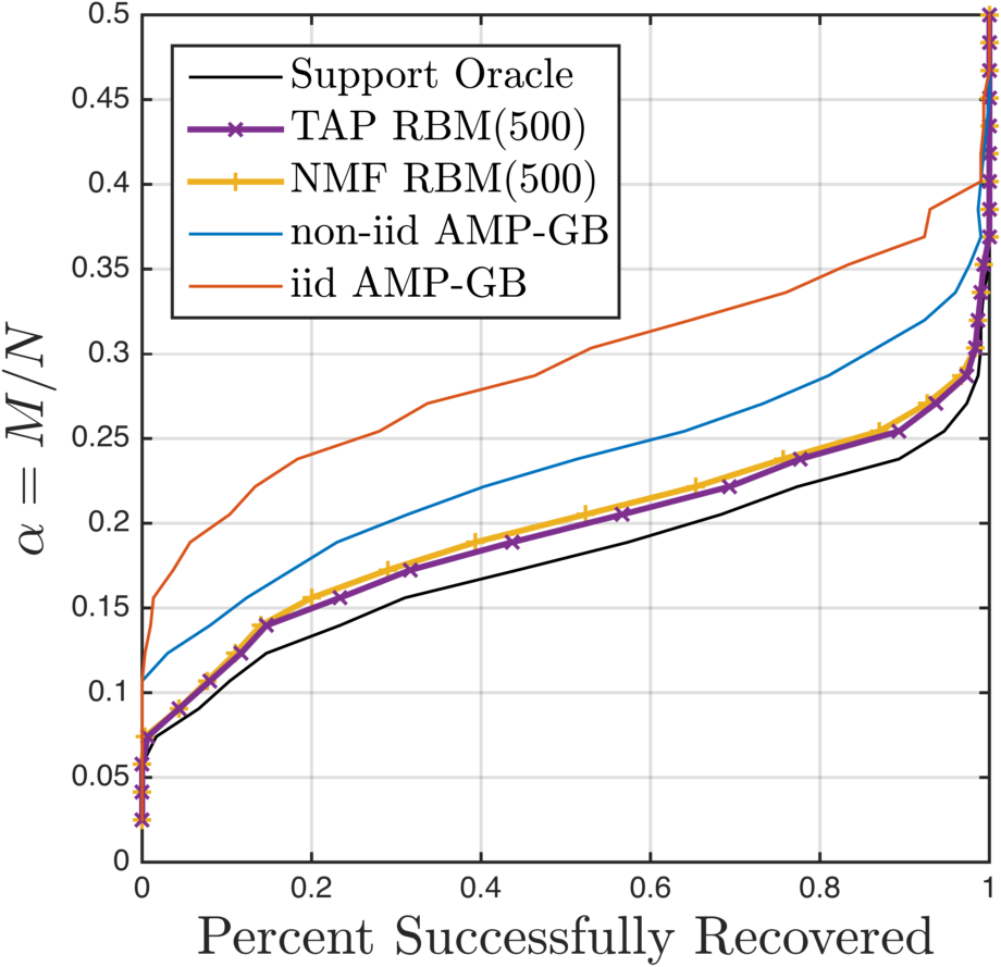
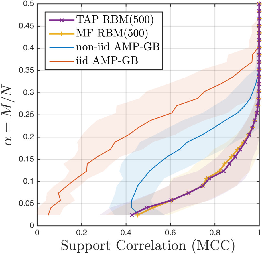
Figure 2: Comparison of MNIST reconstruction performance over 300 test set digits over the measurement rate $\alpha$. For both charts, lower curves represent greater reconstruction performance. (Left) Percentage of test set digit images successfully (MSE $\leq 10^{-4}$) recovered. Note that the AMP-RBM model comes very close to the oracle reconstruction performance bound for this test set. (Right) Correlation, in terms of MCC, between the recovered support and the true digit image support. Here, the solid lines represent the average correlation at each tested $\alpha$, while the solid regions represent the range of one standard deviation of the correlations over the test set.

Figure 3: Visual comparison of reconstructions for four test digits across $\alpha$ for the same experimental settings. The rows of each box, from top to bottom, correspond to the reconstructions providied by i.i.d. AMP-GB, non-i.i.d. AMP-GB, the proposed approach with NMF RBM factorization, and the proposed approach with TAP RBM factorization, respectively. The columns of each box, from left to right, represent the values $\alpha=0.025,0.074,0.123,0.172,0.222,0.271,0.320,0.369,0.418,0.467$. The advantages provided by the proposed approach are clearly seen by comparing the last row to the first one. The digits shown have $\rho=0.342$ (top left), $\rho=0.268$ (bottom left), $\rho=0.214$ (top right), and $\rho=0.162$ (bottom right). The vertical blue line represents the $\alpha=\rho$ oracle exact-reconstruction boundary for each reconstruction task.

We compare the following approaches in Fig. 2. First, we show the reconstruction performance of AMP using an i.i.d. GB prior (AMP-GB), assuming that the true image-wide empirical $\rho$ is given as a parameter for each specific test image. Next, we demonstrate a simple modification to this procedure: the GB prior is assumed to be non-i.i.d. and the values of $\left\{\rho_{i}\right\}$ are empirically estimated from the training samples as the probability of each pixel to be non-zero. We expect that our proposed approach should at least perform as well as non-i.i.d. AMP-GB, as this same information should be encoded in $\mathbf{b}^{\rm v}$ for a properly trained RBM model. Hence, this approach should correspond to an RBM with zero couplings. We also show the performance of the proposed approach: AMP used in conjunction with the RBM support model. We present results for both the NMF and TAP factorizations of the RBM. For the AMP-RBM approaches, we start persistence after AMP 50 iterations. For all tested approaches, we assume that $\Delta$ is known to the reconstruction algorithms, as well as the prior parameters $\mu$ and $\sigma^{2}$. This is not a strict requirement, however, as channel and prior parameters can be estimated within the AMP iteration if so desired [14].

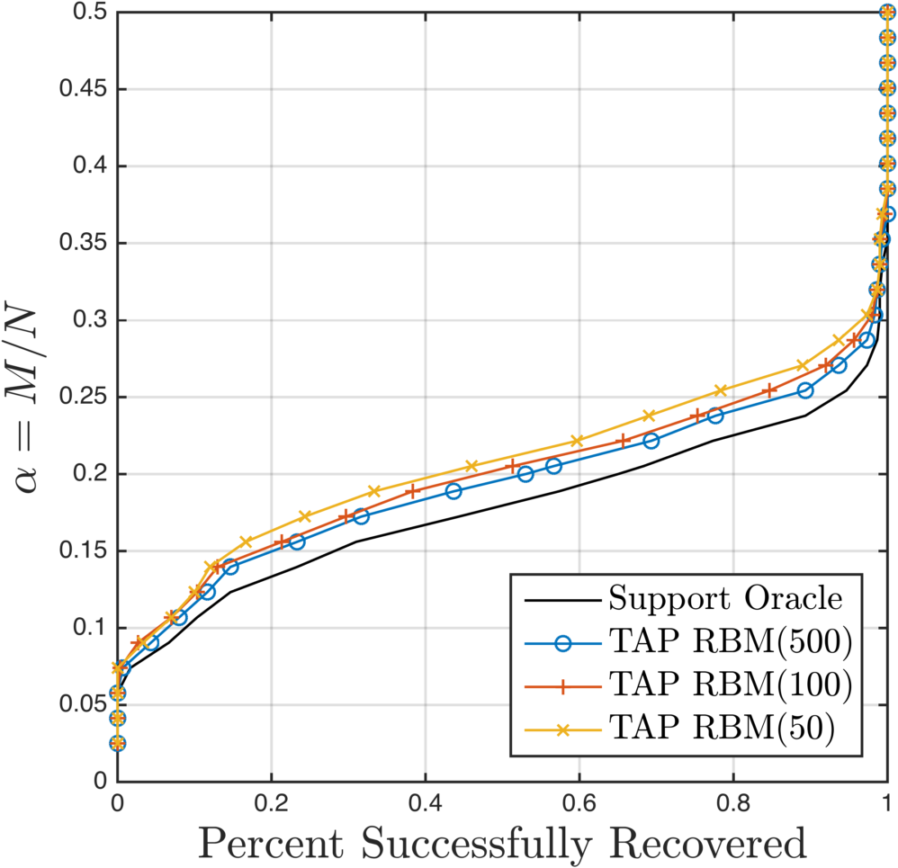
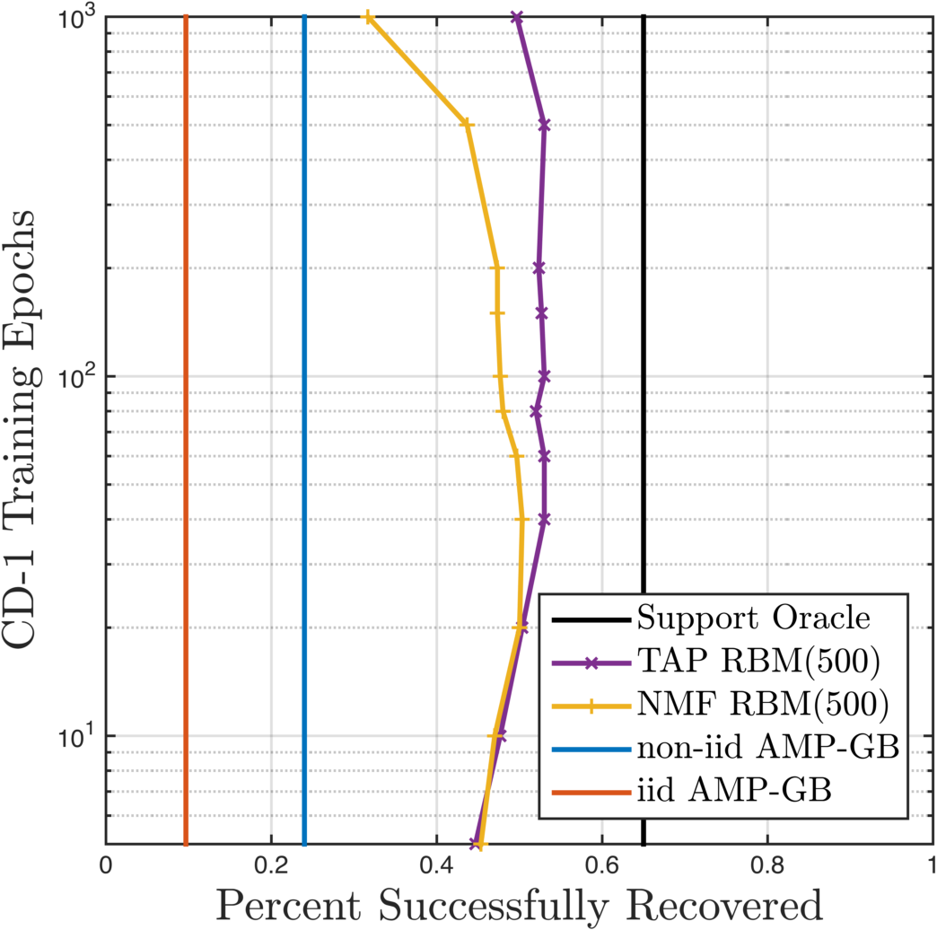
Figure 4: (Left) Test set reconstruction performance for varying numbers of RBM hidden units. One can clearly see in increase in reconstruction performance as the RBM model complexity increases. (Right) Test set reconstruction performance at $\alpha=0.2$ as a function of the number of epochs, from 5 to 1000, used to learn a 500 hidden unit RBM model. Note the sensitivity of the NMF RBM factorization to model over-fitting.

In the left panel of Fig. 2, we present the percentage of successfully recovered test set digit images of the 300 digit images tested. A successful reconstruction is denoted as one which achieves MSE $\leq 10^{-4}$. It is easily observable from these results that leveraging a non-i.i.d. support prior does indeed provide drastic performance improvements, as even the simple non-i.i.d. version of AMP-GB recovers significantly more digits than i.i.d. AMP-GB. We also see that by using the RBM model of the support, along with a TAP-based support probability estimation, we are able to improve upon this simple approach. For example, at $\alpha=0.22$, by using the RBM support prior in conjunction with TAP factorization we are able to recover an additional $56.0\%$ of the test set than with no support information, and an additional $29\%$ than when using only empirical per-coefficient support probabilities. The fact that both RBM-AMP approaches improve on non-i.i.d. AMP-GB demonstrates that the learned support correlations are genuinely providing useful information during the AMP CS reconstruction procedure. We also note that the $2^{{\rm nd}}$-order TAP factorization provides reconstruction performance on this test set which is either equal to, or better than, the NMF factorization, at the cost of an additional matrix-vector multiplication at each iteration of the RBM factorization. To demonstrate how these approaches compare with maximum achievable performance, we also show the support oracle performance, which corresponds to the percentage of test samples for which $\rho\leq\alpha$. The proposed AMP-RBM approach, for the given RBM support model, closes the gap to oracle performance.

In the right panel of Fig. 2, we show the performance of the support estimation in terms of the Matthews Correlation Coefficient (MCC) which is calculated from the $2\times 2$ confusion matrix of estimated support and the true support. We observe from this chart that, even though measurement rate might be so low as to prevent an accurate reconstruction in terms of MSE, the estimated support of the recovered image may indeed be highly correlated with the true image. However, the values of the these on-support coefficients will not be correctly estimated in this regime. The estimated support may still be used for certain tasks in this case, such as classification. More visual evidence of this effect can be seen in Fig. 3, were we see, even to the down to the extreme limit of $\alpha<0.1$, the support of the AMP-RBM recovered images are still quite correlated with the true image. For non-i.i.d. AMP-GB, the effect of the prior effectively forces the support to the central region of the image, and for i.i.d. AMP-GB, the support information is completely lost, having almost zero correlation with the true image.

It is also of interest to analyze the effect of RBM training and model parameters on the performance of the proposed approach. Indeed, it is curious to note exactly how well trained the RBM must be in order to obtain the performance demonstrated above. In the right panel of Fig. 4 we see that a lightly trained, here on the order of 40 epochs, RBM attains maximal performance, showing that an overwrought training procedure is not necessary in order to obtain significant performance improvements for CS reconstruction. Additionally, in the left panel of Fig. 4 we see that increasing the complexity of the RBM model, and therefore more accurately estimating the joint support probability,increases reconstruction performance, showing that more complex RBMs, perhaps even stacked RBM models, may have the potential to further improve upon these results.

Lastly, in terms of computational efficiency and scalability, the inclusion of the inner RBM factorization loop does increase the computational burden of the reconstruction in proportion to the number of hidden units and the number of factorization iterations required for convergence. However, these iterations are computationally light in comparison to the AMP FPI and so the use of the RBM support prior is not unduly burdensome.

6 Conclusion

In this work we show that using an RBM-based prior on the signal support, when learned properly, can provide CS reconstruction performance superior to that of both simple i.i.d. and empirical non-i.i.d. sparsity assumptions for a message passing approach such as AMP. The implications of such an approach are large as these results pave the way for the introduction of much more complex and deep-learned priors. Such priors can be applied to the signal support as we have done here, or further modifications can be made to adapt the AMP framework to the use of RBMs with real-valued visible layers. Such priors would even aid in moving past the $M=K$ oracle support transition.

Additionally, a number of interesting generalizations of our approach are possible. While the experiments we present here are only concerned with linear projections observed through an AWGN channel, much more general, non-linear, observation models can be used moving from AMP to GAMP [11]. Our approach can be then readily applied with essentially no modification to the algorithm. With the successful application of statistical physics tools to signal reconstruction, as was done in applying TAP to derive AMP, similar approaches could be adapted to produce even better learning algorithms for single and stacked RBMs. Perhaps such future works might allow for the estimation of the RBM model in parallel with signal reconstruction.

References

- [1] E. Candès and J. Romberg, “Signal recovery from random projections,” in Computational Imaging III. San Jose, CA: Proc. SPIE 5674, Mar. 2005, pp. 76–86.
- [2] D. L. Donoho, A. Maleki, and A. Montanari, “Message-passing algorithms for compressed sensing,” Proc. National Academy of Sciences of the U.S.A., vol. 106, no. 45, p. 18914, 2009.
- [3] M. A. Borgerding, P. Schniter, and S. Rangan, “Generalized approximate message passing for cosparse analysis compressive sensing,” arXiv preprint, no. 1312.3968 [cs.IT], December 2013.
- [4] S. Rangan, A. K. Fletcher, V. K. Goyal, and P. Schniter, “Hybrid approximate message passing with applications to structured sparsity,” arXiv preprint, no. 1111.2581 [cs.IT], November 2011.
- [5] P. Smolensky, Information Processing in Dynamical Systems: Foundations of Harmony Theory, ser. Parallel Distributed Porcessing: Explorations in the Microsctructure of Cognition. MIT Press, 1986, ch. 6, pp. 194–281.
- [6] G. E. Hinton, “Training products of experts by minimizing contrastive divergence,” Neural Computation, vol. 14, no. 8, pp. 1771–1800, August 2002.
- [7] Y. Bengio, “Learning deep architectures for AI,” Foundations and Trends® in Machine Learning, vol. 2, no. 1, pp. 1–127, 2009.
- [8] J. Pearl, “Reverend Bayes on inference engines: A distributed hierarchical approach,” in Proc. American Association of Art. Int. Nat. Conf. on AI, Pittsburgh, PA, USA, 1982, pp. 133–136.
- [9] M. Mézard and A. Montanari, Information, Physics, and Computation. OUP, 2009.
- [10] D. L. Donoho, A. Maleki, and A. Montanari, “Message-passing algorithms for compressed sensing: I. motivation and construction,” in Proc. IEEE Info. Theory Workshop, 2010, pp. 1–5.
- [11] S. Rangan, “Generalized approximate message passing for estimation with random linear mixing,” in Proc. IEEE Intl. Symp. on Info. Theory, 2011, p. 2168.
- [12] J. P. Vila and P. Schniter, “Expectation-maximization gaussian-mixture approximate message passing,” IEEE Trans. on Signal Processing, vol. 61, no. 19, pp. 4658–4672, 2013.
- [13] F. Krzakala, M. Mézard, F. Sausset, Y. Sun, and L. Zdeborová, “Statistical physics-based reconstruction in compressed sensing,” Phys. Rev. X, vol. 2, p. 021005, 2012.
- [14] ——, “Probabilistic reconstruction in compressed sensing: Algorithms, phase diagrams, and threshold achieving matrices,” Journal of Statistical Mechanics: Theory and Experiment, vol. 2012, no. 8, p. P08009, August 2012.
- [15] P. Schniter, “Turbo reconstruction of structured sparse signals,” in Proc. Conf. on Info. Sciences and Systems. IEEE, 2010, pp. 1–6.
- [16] A. Drémeau, C. Herzet, and L. Daudet, “Boltzmann machine and mean-field approximation for structured sparse decompositions,” IEEE Trans. on Signal Processing, vol. 60, no. 7, pp. 3425–3438, 2012.
- [17] D. J. Thouless, P. W. Anderson, and R. G. Palmer, “Solution of ‘solvable model of a spin-glass’,” Phil. Mag., vol. 35, pp. 593–601, 1977.
- [18] M. Mézard, G. Parisi, and M. A. Virasoro, Spin Glass Theory and Beyond. World Scientific, 1987.
- [19] J. Yedidia, “An idiosyncratic journey beyond mean field theory,” in Advanced Mean Field Methods, Theory and Practice, M. Opper and D. Saad, Eds. The MIT Press, 2001, pp. 21–36.
- [20] M. Gabrié, E. W. Tramel, and F. Krzakala, “Training restricted Boltzmann machines via the Thouless-Andreson-Palmer free energy,” in Proc. Conf. on Neural Info. Processing Sys. (NIPS), Montreal, Canada, June 2015.
- [21] T. Plefka, “Convergence condition of the TAP equation for the infinite-ranged ising spin glass model,” Journal of Physics A: Mathematical and General, vol. 15, no. 6, p. 1971, 1982.
- [22] T. Tieleman, “Training restricted Boltzmann machines using approximations to the likelihood gradient,” in Proc. Intl. Conf. on Machine Learning, July 2008, pp. 1064–1071.
- [23] G. Hinton, “A practical guide to training restricted Boltzmann machines,” Momentum, vol. 9, no. 1, p. 926, 2010.
- [24] A. Fischer, “Training restricted Boltzmann machines,” Ph.D. dissertation, University of Copenhagen, Copenhagen, Denmark, June 2014.