Rectified Factor Networks
Abstract
We propose rectified factor networks (RFNs) to efficiently construct very sparse, non-linear, high-dimensional representations of the input. RFN models identify rare and small events in the input, have a low interference between code units, have a small reconstruction error, and explain the data covariance structure. RFN learning is a generalized alternating minimization algorithm derived from the posterior regularization method which enforces non-negative and normalized posterior means. We proof convergence and correctness of the RFN learning algorithm.
On benchmarks, RFNs are compared to other unsupervised methods like autoencoders, RBMs, factor analysis, ICA, and PCA. In contrast to previous sparse coding methods, RFNs yield sparser codes, capture the data’s covariance structure more precisely, and have a significantly smaller reconstruction error. We test RFNs as pretraining technique for deep networks on different vision datasets, where RFNs were superior to RBMs and autoencoders. On gene expression data from two pharmaceutical drug discovery studies, RFNs detected small and rare gene modules that revealed highly relevant new biological insights which were so far missed by other unsupervised methods.
1 Introduction
The success of deep learning is to a large part based on advanced and efficient input representations [1, 2, 3, 4]. These representations are sparse and hierarchical. Sparse representations of the input are in general obtained by rectified linear units (ReLU) [5, 6] and dropout [7]. The key advantage of sparse representations is that dependencies between coding units are easy to model and to interpret. Most importantly, distinct concepts are much less likely to interfere in sparse representations. Using sparse representations, similarities of samples often break down to co-occurrences of features in these samples. In bioinformatics sparse codes excelled in biclustering of gene expression data [8] and in finding DNA sharing patterns between humans and Neanderthals [9].
Representations learned by ReLUs are not only sparse but also non-negative. Non-negative representations do not code the degree of absence of events or objects in the input. As the vast majority of events is supposed to be absent, to code for their degree of absence would introduce a high level of random fluctuations. We also aim for non-linear input representations to stack models for constructing hierarchical representations. Finally, the representations are supposed to have a large number of coding units to allow coding of rare and small events in the input. Rare events are only observed in few samples like seldom side effects in drug design, rare genotypes in genetics, or small customer groups in e-commerce. Small events affect only few input components like pathways with few genes in biology, few relevant mutations in oncology, or a pattern of few products in e-commerce. In summary, our goal is to construct input representations that (1) are sparse, (2) are non-negative, (3) are non-linear, (4) use many code units, and (5) model structures in the input data (see next paragraph).
Current unsupervised deep learning approaches like autoencoders or restricted Boltzmann machines (RBMs) do not model specific structures in the data. On the other hand, generative models explain structures in the data but their codes cannot be enforced to be sparse and non-negative. The input representation of a generative model is its posterior’s mean, median, or mode, which depends on the data. Therefore sparseness and non-negativity cannot be guaranteed independent of the data. For example, generative models with rectified priors, like rectified factor analysis, have zero posterior probability for negative values, therefore their means are positive and not sparse [10, 11]. Sparse priors do not guarantee sparse posteriors as seen in the experiments with factor analysis with Laplacian and Jeffrey’s prior on the factors (see Tab. 1). To address the data dependence of the code, we employ the posterior regularization method [12]. This method separates model characteristics from data dependent characteristics that are enforced by constraints on the model’s posterior.
We aim at representations that are feasible for many code units and massive datasets, therefore the computational complexity of generating a code is essential in our approach. For non-Gaussian priors, the computation of the posterior mean of a new input requires either to numerically solve an integral or to iteratively update variational parameters [13]. In contrast, for Gaussian priors the posterior mean is the product between the input and a matrix that is independent of the input. Still the posterior regularization method leads to a quadratic (in the number of coding units) constrained optimization problem in each E-step (see Eq. (3) below). To speed up computation, we do not solve the quadratic problem but perform a gradient step. To allow for stochastic gradients and fast GPU implementations, also the M-step is a gradient step. These E-step and M-step modifications of the posterior regularization method result in a generalized alternating minimization (GAM) algorithm [12]. We will show that the GAM algorithm used for RFN learning (i) converges and (ii) is correct. Correctness means that the RFN codes are non-negative, sparse, have a low reconstruction error, and explain the covariance structure of the data.
2 Rectified Factor Network
Our goal is to construct representations of the input that (1) are sparse, (2) are non-negative, (3) are non-linear, (4) use many code units, and (5) model structures in the input. Structures in the input are identified by a generative model, where the model assumptions determine which input structures to explain by the model. We want to model the covariance structure of the input, therefore we choose maximum likelihood factor analysis as model. The constraints on the input representation are enforced by the posterior regularization method [12]. Non-negative constraints lead to sparse and non-linear codes, while normalization constraints scale the signal part of each hidden (code) unit. Normalizing constraints avoid that generative models explain away rare and small signals by noise. Explaining away becomes a serious problem for models with many coding units since their capacities are not utilized. Normalizing ensures that all hidden units are used but at the cost of coding also random and spurious signals. Spurious and true signals must be separated in a subsequent step either by supervised techniques, by evaluating coding units via additional data, or by domain experts.
A generative model with hidden units and data is defined by its prior and its likelihood . The full model distribution can be expressed by the model’s posterior and its evidence (marginal likelihood) : . The representation of input is the posterior’s mean, median, or mode. The posterior regularization method introduces a variational distribution from a family , which approximates the posterior . We choose to constrain the posterior means to be non-negative and normalized. The full model distribution contains all model assumptions and, thereby, defines which structures of the data are modeled. contains data dependent constraints on the posterior, therefore on the code.
For data , the posterior regularization method maximizes the objective [12]:
| (1) | ||||
where is the Kullback-Leibler distance. Maximizing achieves two goals simultaneously: (1) extracting desired structures and information from the data as imposed by the generative model and (2) ensuring desired code properties via .
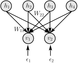
The factor analysis model extracts the covariance structure of the data. The prior of the hidden units (factors) and the noise of visible units (observations) are independent. The model parameters are the weight (loading) matrix and the noise covariance matrix . We assume diagonal to explain correlations between input components by the hidden units and not by correlated noise. The factor analysis model is depicted in Fig. 1. Given the mean-centered data , the posterior is Gaussian with mean vector and covariance matrix :
| (2) |
A rectified factor network (RFN) consists of a single or stacked factor analysis model(s) with constraints on the posterior. To incorporate the posterior constraints into the factor analysis model, we use the posterior regularization method that maximizes the objective given in Eq. (1) [12]. Like the expectation-maximization (EM) algorithm, the posterior regularization method alternates between an E-step and an M-step. Minimizing the first of Eq. (1) with respect to leads to a constrained optimization problem. For Gaussian distributions, the solution with and from Eq. (2) is with and the quadratic problem:
| (3) |
where “” is component-wise. This is a constraint non-convex quadratic optimization problem in the number of hidden units which is too complex to be solved in each EM iteration. Therefore, we perform a step of the gradient projection algorithm [14, 15], which performs first a gradient step and then projects the result to the feasible set. We start by a step of the projected Newton method, then we try the gradient projection algorithm, thereafter the scaled gradient projection algorithm with reduced matrix [16] (see also [15]). If these methods fail to decrease the objective in Eq. (3), we use the generalized reduced method [17]. It solves each equality constraint for one variable and inserts it into the objective while ensuring convex constraints. Alternatively, we use Rosen’s gradient projection method [18] or its improvement [19]. These methods guarantee a decrease of the E-step objective.
Since the projection by Eq. (8) is very fast, the projected Newton and projected gradient update is very fast, too. A projected Newton step requires steps (see Eq. (9) and defined in Theorem 1), a projected gradient step requires steps, and a scaled gradient projection step requires steps. The RFN complexity per iteration is (see Alg. 1). In contrast, a quadratic program solver typically requires for the variables (the means of the hidden units for all samples) steps to find the minimum [20]. We exemplify these values on our benchmark datasets MNIST (k, ) and CIFAR (k, ). The speedup with projected Newton or projected gradient in contrast to a quadratic solver is , which gives speedup ratios of for MNIST and for CIFAR. These speedup ratios show that efficient E-step updates are essential for RFN learning. Furthermore, on our computers, RAM restrictions limited quadratic program solvers to problems with k.
The M-step decreases the expected reconstruction error
| (4) | ||||
from Eq. (1) with respect to the model parameters and . Definitions of , and are given in Alg. 1. The M-step performs a gradient step in the Newton direction, since we want to allow stochastic gradients, fast GPU implementation, and dropout regularization. The Newton step is derived in the supplementary which gives further details, too. Also in the E-step, RFN learning performs a gradient step using projected Newton or gradient projection methods. These projection methods require the Euclidean projection of the posterior means onto the non-convex feasible set:
| (5) |
The following Theorem 1 gives the Euclidean projection as solution to Eq. (5).
Theorem 1 (Euclidean Projection).
Proof.
See supplementary material. ∎
Using the projection defined in Eq. (8), the E-step updates for the posterior means are:
| (9) |
where we set for the projected Newton method (thus ), and for the projected gradient method . For the scaled gradient projection algorithm with reduced matrix, the -active set for consists of all with . The reduced matrix is the Hessian with -active columns and rows fixed to unit vectors . The resulting algorithm is a posterior regularization method with a gradient based E- and M-step, leading to a generalized alternating minimization (GAM) algorithm [21]. The RFN learning algorithm is given in Alg. 1. Dropout regularization can be included before E-step2 by randomly setting code units to zero with a predefined dropout rate (note that convergence results will no longer hold).
Complexity: objective : ; E-step1: ; projected Newton: ; projected gradient: ; scaled gradient projection: ; E-step2: ; M-step: ; overall complexity with projected Newton / gradient for : .
3 Convergence and Correctness of RFN Learning
Convergence of RFN Learning.
Theorem 2 (RFN Convergence).
The rectified factor network (RFN) learning algorithm given in Alg. 1 is a “generalized alternating minimization” (GAM) algorithm and converges to a solution that maximizes the objective .
Proof.
We present a sketch of the proof which is given in detail in the supplement. For convergence, we show that Alg. 1 is a GAM algorithm which convergences according to Proposition 5 in [21].
Alg. 1 ensures to decrease the M-step objective which is convex in and . The update with leads to the minimum of the objective. Convexity of the objective guarantees a decrease in the M-step for if not in a minimum. Alg. 1 ensures to decrease the E-step objective by using gradient projection methods. All other requirements for GAM convergence are also fulfilled. ∎
Correctness of RFN Learning.
The goal of the RFN algorithm is to explain the data and its covariance structure. The expected approximation error is defined in line 14 of Alg. 1. Theorem 3 states that the RFN algorithm is correct, that is, it explains the data (low reconstruction error) and captures the covariance structure as good as possible.
Theorem 3 (RFN Correctness).
The fixed point of Alg. 1 minimizes given and by ridge regression with
| (10) |
where . The model explains the data covariance matrix by
| (11) |
up to an error, which is quadratic in for . The reconstruction error is quadratic in for .
Proof.
The fixed point equation for the update is . Using the definition of and , we have . is the ridge regression solution of
| (12) |
where is the trace. After multiplying out all in , we obtain:
| (13) |
For the fixed point of , the update rule gives: . Thus, minimizes given and . Multiplying the Woodbury identity for from left and right by gives
| (14) |
Inserting this into the expression for and taking the trace gives
| (15) |
Therefore for the error is quadratic in . follows from fixed point equation . Using this and Eq. (14), Eq. (13) is
| (16) |
Using the trace norm (nuclear norm or Ky-Fan n-norm) on matrices, Eq. (15) states that the left hand side of Eq. (16) is quadratic in for . The trace norm of a positive semi-definite matrix is its trace and bounds the Frobenius norm [23]. Thus, for , the covariance is approximated up to a quadratic error in according to Eq. (11). The diagonal is exactly modeled. ∎
Since the minimization of the expected reconstruction error is based on , the quality of reconstruction depends on the correlation between and . We ensure maximal information in on by the I-projection (the minimal Kullback-Leibler distance) of the posterior onto the family of rectified and normalized Gaussian distributions.
4 Experiments
| undercomplete 50 code units | complete 100 code units | overcomplete 150 code units | |||||||
| SP | ER | CO | SP | ER | CO | SP | ER | CO | |
| RFN | 750 | 2493 | 1083 | 811 | 689 | 266 | 851 | 176 | 76 |
| RFNn | 740 | 2954 | 1404 | 790 | 1855 | 593 | 800 | 1424 | 352 |
| DAE | 660 | 2513 | — | 690 | 1472 | — | 710 | 1302 | — |
| RBM | 151 | 3104 | — | 71 | 2874 | — | 50 | 2864 | — |
| FAsp | 401 | 99963 | 99999 | 630 | 99965 | 99999 | 800 | 99965 | 99999 |
| FAlap | 40 | 2396 | 34119 | 60 | 464 | 98545 | 40 | 464 | 97653 |
| ICA | 20 | 1742 | — | 31 | 00 | — | 31 | 00 | — |
| SFA | 10 | 2185 | 943 | 10 | 161 | 1145 | 10 | 161 | 2857 |
| FA | 10 | 2184 | 903 | 10 | 161 | 834 | 10 | 161 | 2636 |
| PCA | 00 | 1742 | — | 20 | 00 | — | 20 | 00 | — |
RFNs vs. Other Unsupervised Methods.
We assess the performance of rectified factor
networks (RFNs) as unsupervised methods for data representation.
We compare
(1) RFN: rectified factor networks,
(2) RFNn: RFNs without normalization,
(3) DAE: denoising autoencoders with ReLUs,
(4) RBM: restricted Boltzmann machines with Gaussian visible units,
(5) FAsp: factor analysis with Jeffrey’s prior () on the hidden units which is
sparser than a Laplace prior,
(6) FAlap: factor analysis with Laplace prior on the
hidden units,
(7) ICA: independent component analysis by FastICA [24],
(8) SFA: sparse factor analysis with a Laplace prior on the parameters,
(9) FA: standard factor analysis,
(10) PCA: principal component analysis.
The number of components are fixed to 50, 100 and 150 for each method.
We generated nine different benchmark datasets (D1 to D9),
where each dataset consists of 100 instances. Each instance
has 100 samples and 100 features resulting in a
100100 matrix.
Into these matrices, biclusters are implanted [8].
A bicluster is a pattern of particular features which is found in
particular samples like a pathway activated in some samples.
An optimal representation will only code the biclusters
that are present in a sample.
The datasets have different noise levels and different bicluster sizes.
Large biclusters have 20–30 samples and 20–30 features,
while small biclusters 3–8 samples and 3–8 features.
The pattern’s signal strength in a particular sample
was randomly chosen according to the Gaussian .
Finally, to each matrix, zero-mean Gaussian
background noise was added with standard deviation 1, 5, or 10.
The datasets are characterized by Dx= with
background noise , number of large biclusters ,
and the number of small biclusters :
D1=(1,10,10),
D2=(5,10,10),
D3=(10,10,10),
D4=(1,15,5),
D5=(5,15,5),
D6=(10,15,5),
D7=(1,5,15),
D8=(5,5,15),
D9=(10,5,15).
We evaluated the methods according to the (1) sparseness of the
components, the (2) input reconstruction error from the code,
and the (3) covariance reconstruction error for generative models.
For RFNs sparseness is the percentage of the components that are
exactly 0, while
for others methods it is the percentage of components with an absolute value
smaller than 0.01.
The reconstruction error is the sum
of the squared errors across samples.
The covariance reconstruction error is the Frobenius norm
of the difference between model and data covariance.
See supplement for more details on the data and for
information on hyperparameter selection for the different methods.
Tab. 1 gives averaged results for models with 50
(undercomplete), 100 (complete) and 150 (overcomplete) coding units.
Results are the mean of 900 instances consisting of 100 instances for
each dataset D1 to D9.
In the supplement, we separately
tabulate the results for D1 to D9 and confirm them
with different noise levels.
FAlap did not yield sparse codes since the variational
parameter did not push the absolute representations below the
threshold of 0.01.
The variational approximation to the Laplacian is a Gaussian
distribution [13].
RFNs had the sparsest code, the lowest
reconstruction error, and the lowest covariance
approximation error of all methods that yielded sparse
representations (SP>10%).
RFN Pretraining for Deep Nets.
We assess the performance of rectified factor
networks (RFNs) if used for pretraining of
deep networks.
Stacked RFNs are obtained by first training a single layer RFN
and then passing on the resulting representation as input for training
the next RFN.
The deep network architectures use a RFN pretrained
first layer (RFN-1) or stacks of 3 RFNs giving a 3-hidden layer network.
The classification performance of deep networks with RFN pretrained layers
was compared to
(i) support vector machines,
(ii) deep networks pretrained by stacking denoising autoencoders (SDAE),
(iii) stacking regular autoencoders (SAE),
(iv) restricted Boltzmann machines (RBM), and
(v) stacking restricted Boltzmann machines (DBN).
| Dataset | SVM | RBM | DBN | SAE | SDAE | RFN | |
|---|---|---|---|---|---|---|---|
| MNIST | 50k-10k-10k | 1.400.23 | 1.210.21 | 1.240.22 | 1.400.23 | 1.280.22 | 1.270.22 (1) |
| basic | 10k-2k-50k | 3.030.15 | 3.940.17 | 3.110.15 | 3.460.16 | 2.840.15 | 2.660.14 (1) |
| bg-rand | 10k-2k-50k | 14.580.31 | 9.800.26 | 6.730.22 | 11.280.28 | 10.300.27 | 7.940.24 (3) |
| bg-img | 10k-2k-50k | 22.610.37 | 16.150.32 | 16.310.32 | 23.000.37 | 16.680.33 | 15.660.32 (1) |
| rect | 1k-0.2k-50k | 2.150.13 | 4.710.19 | 2.600.14 | 2.410.13 | 1.990.12 | 0.630.06 (1) |
| rect-img | 10k-2k-50k | 24.040.37 | 23.690.37 | 22.500.37 | 24.050.37 | 21.590.36 | 20.770.36 (1) |
| convex | 10k-2k-50k | 19.130.34 | 19.920.35 | 18.630.34 | 18.410.34 | 19.060.34 | 16.410.32 (1) |
| NORB | 19k-5k-24k | 11.60.40 | 8.310.35 | - | 10.100.38 | 9.500.37 | 7.000.32 (1) |
| CIFAR | 40k-10k-10k | 62.70.95 | 40.390.96 | 43.380.97 | 43.250.97 | - | 41.290.95 (1) |
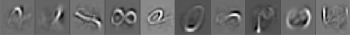
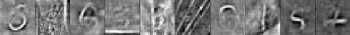
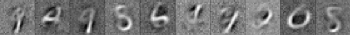
The benchmark datasets and results are taken from previous publications [25, 26, 27, 28] and contain: (i) MNIST (original MNIST), (ii) basic (a smaller subset of MNIST for training), (iii) bg-rand (MNIST with random noise background), (iv) bg-img (MNIST with random image background), (v) rect (discrimination between tall and wide rectangles), (vi) rect-img (discrimination between tall and wide rectangular images overlayed on random background images), (vii) convex (discrimination between convex and concave shapes), (viii) CIFAR-10 (60k color images in 10 classes), and (ix) NORB (29,160 stereo image pairs of 5 generic categories). For each dataset its size of training, validation and test set is given in the second column of Tab. 2. As preprocessing we only performed median centering. Model selection is based on the validation set performance [26]. The RFNs hyperparameters are (i) the number of units per layer from and (ii) the dropout rate from . The learning rate was fixed to its default value of . For supervised fine-tuning with stochastic gradient descent, we selected the learning rate from , the masking noise from , and the number of layers from . Fine-tuning was stopped based on the validation set performance, following [26]. The test error rates together with the 95% confidence interval (computed according to [26]) for deep network pretraining by RFNs and other methods are given in Tab. 2. Fig. 2 shows learned filters. The result of the best performing method is given in bold, as well as the result of those methods for which confidence intervals overlap. RFNs were only once significantly worse than the best method but still the second best. In six out of the nine experiments RFNs performed best, where in four cases it was significantly the best.
RFNs in Drug Discovery.
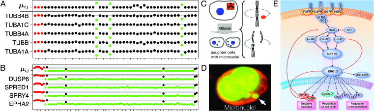
Using RFNs we analyzed gene expression datasets of two projects in the lead optimization phase of a big pharmaceutical company [29]. The first project aimed at finding novel antipsychotics that target PDE10A. The second project was an oncology study that focused on compounds inhibiting the FGF receptor. In both projects, the expression data was summarized by FARMS [30] and standardized. RFNs were trained with 500 hidden units, no masking noise, and a learning rate of . The identified transcriptional modules are shown in Fig. 3. Panels A and B illustrate that RFNs found rare and small events in the input. In panel A only a few drugs are genotoxic (rare event) by downregulating the expression of a small number of tubulin genes (small event). The genotoxic effect stems from the formation of micronuclei (panel C and D) since the mitotic spindle apparatus is impaired. Also in panel B, RFN identified a rare and small event which is a transcriptional module that has a negative feedback to the MAPK signaling pathway. Rare events are unexpectedly inactive drugs (black dots), which do not inhibit the FGF receptor. Both findings were not detected by other unsupervised methods, while they were highly relevant and supported decision-making in both projects [29].
5 Conclusion
We have introduced rectified factor networks (RFNs) for constructing very sparse and non-linear input representations with many coding units in a generative framework. Like factor analysis, RFN learning explains the data variance by its model parameters. The RFN learning algorithm is a posterior regularization method which enforces non-negative and normalized posterior means. We have shown that RFN learning is a generalized alternating minimization method which can be proved to converge and to be correct. RFNs had the sparsest code, the lowest reconstruction error, and the lowest covariance approximation error of all methods that yielded sparse representations (SP10%). RFNs have shown that they improve performance if used for pretraining of deep networks. In two pharmaceutical drug discovery studies, RFNs detected small and rare gene modules that were so far missed by other unsupervised methods. These gene modules were highly relevant and supported the decision-making in both studies. RFNs are geared to large datasets, sparse coding, and many representational units, therefore they have high potential as unsupervised deep learning techniques.
Acknowledgment.
The Tesla K40 used for this research was donated by the NVIDIA Corporation.
References
- [1] G. E. Hinton and R. Salakhutdinov. Reducing the dimensionality of data with neural networks. Science, 313(5786):504–507, 2006.
- [2] Y. Bengio, P. Lamblin, D. Popovici, and H. Larochelle. Greedy layer-wise training of deep networks. In B. Schölkopf, J. C. Platt, and T. Hoffman, editors, NIPS, pages 153–160. MIT Press, 2007.
- [3] J. Schmidhuber. Deep learning in neural networks: An overview. Neural Networks, 61:85–117, 2015.
- [4] Y. LeCun, Y. Bengio, and G. Hinton. Deep learning. Nature, 521(7553):436–444, 2015.
- [5] V. Nair and G. E. Hinton. Rectified linear units improve restricted Boltzmann machines. In ICML, pages 807–814. Omnipress 2010, ISBN 978-1-60558-907-7, 2010.
- [6] X. Glorot, A. Bordes, and Y. Bengio. Deep sparse rectifier neural networks. In AISTATS, volume 15, pages 315–323, 2011.
- [7] N. Srivastava, G. Hinton, A. Krizhevsky, I. Sutskever, and R. Salakhutdinov. Dropout: A simple way to prevent neural networks from overfitting. Journal of Machine Learning Research, 15:1929–1958, 2014.
- [8] S. Hochreiter, U. Bodenhofer, et al. FABIA: factor analysis for bicluster acquisition. Bioinformatics, 26(12):1520–1527, 2010.
- [9] S. Hochreiter. HapFABIA: Identification of very short segments of identity by descent characterized by rare variants in large sequencing data. Nucleic Acids Res., 41(22):e202, 2013.
- [10] B. J. Frey and G. E. Hinton. Variational learning in nonlinear Gaussian belief networks. Neural Computation, 11(1):193–214, 1999.
- [11] M. Harva and A. Kaban. Variational learning for rectified factor analysis. Signal Processing, 87(3):509–527, 2007.
- [12] K. Ganchev, J. Graca, J. Gillenwater, and B. Taskar. Posterior regularization for structured latent variable models. Journal of Machine Learning Research, 11:2001–2049, 2010.
- [13] J. Palmer, D. Wipf, K. Kreutz-Delgado, and B. Rao. Variational EM algorithms for non-Gaussian latent variable models. In NIPS, volume 18, pages 1059–1066, 2006.
- [14] D. P. Bertsekas. On the Goldstein-Levitin-Polyak gradient projection method. IEEE Trans. Automat. Control, 21:174–184, 1976.
- [15] C. T. Kelley. Iterative Methods for Optimization. Society for Industrial and Applied Mathematics (SIAM), Philadelphia, 1999.
- [16] D. P. Bertsekas. Projected Newton methods for optimization problems with simple constraints. SIAM J. Control Optim., 20:221–246, 1982.
- [17] J. Abadie and J. Carpentier. Optimization, chapter Generalization of the Wolfe Reduced Gradient Method to the Case of Nonlinear Constraints. Academic Press, 1969.
- [18] J. B. Rosen. The gradient projection method for nonlinear programming. part ii. nonlinear constraints. Journal of the Society for Industrial and Applied Mathematics, 9(4):514–532, 1961.
- [19] E. J. Haug and J. S. Arora. Applied optimal design. J. Wiley & Sons, New York, 1979.
- [20] A. Ben-Tal and A. Nemirovski. Interior Point Polynomial Time Methods for Linear Programming, Conic Quadratic Programming, and Semidefinite Programming, chapter 6, pages 377–442. Society for Industrial and Applied Mathematics, 2001.
- [21] A. Gunawardana and W. Byrne. Convergence theorems for generalized alternating minimization procedures. Journal of Machine Learning Research, 6:2049–2073, 2005.
- [22] W. I. Zangwill. Nonlinear Programming: A Unified Approach. Prentice Hall, Englewood Cliffs, N.J., 1969.
- [23] N. Srebro. Learning with Matrix Factorizations. PhD thesis, Department of Electrical Engineering and Computer Science, Massachusetts Institute of Technology, 2004.
- [24] A. Hyvärinen and E. Oja. A fast fixed-point algorithm for independent component analysis. Neural Comput., 9(7):1483–1492, 1999.
- [25] Y. LeCun, F.-J. Huang, and L. Bottou. Learning methods for generic object recognition with invariance to pose and lighting. In Proceedings of the IEEE Conference on Computer Vision and Pattern Recognition (CVPR). IEEE Press, 2004.
- [26] P. Vincent, H. Larochelle, et al. Stacked denoising autoencoders: Learning useful representations in a deep network with a local denoising criterion. JMLR, 11:3371–3408, 2010.
- [27] H. Larochelle, D. Erhan, et al. An empirical evaluation of deep architectures on problems with many factors of variation. In ICML, pages 473–480, 2007.
- [28] A. Krizhevsky. Learning multiple layers of features from tiny images. Master’s thesis, Deptartment of Computer Science, University of Toronto, 2009.
- [29] B. Verbist, G. Klambauer, et al. Using transcriptomics to guide lead optimization in drug discovery projects: Lessons learned from the {QSTAR} project. Drug Discovery Today, 20(5):505 – 513, 2015.
- [30] S. Hochreiter, D.-A. Clevert, and K. Obermayer. A new summarization method for Affymetrix probe level data. Bioinformatics, 22(8):943–949, 2006.
Supplementary Material
appendix.A appendix.B appendix.C appendix.D subsection.D.1 subsection.D.2 appendix.E appendix.F appendix.G appendix.H subsection.H.1 subsection.H.2 subsubsection.H.2.1 subsubsection.H.2.2 thmt@dummyctr.dummy.9 thmt@dummyctr.dummy.10 appendix.I subsection.I.1 subsection.I.2 subsection.I.3 subsubsection.I.3.1 subsubsection.I.3.2 subsection.I.4 subsubsection.I.4.1 section*.19 section*.20 subsubsection.I.4.2 subsection.I.5 subsubsection.I.5.1 subsubsection.I.5.2 subsubsection.I.5.3 appendix.J appendix.K appendix.L appendix.M appendix.N
Appendix S1 Introduction
This supplement contains additional information complementing the main manuscript and is structured as follows: First, the rectified factor network (RFN) learning algorithm with E- and M-step updates, weight decay and dropout regularization is given in Section S2. In Section S3, we proof that the (RFN) learning algorithm is a “generalized alternating minimization” (GAM) algorithm and converges to a solution that maximizes the RFN objective. The correctness of the RFN algorithm is proofed in Section S4. Section S5 describes the maximum likelihood factor analysis model and the model selection by the EM-algorithm. The RFN objective, which has to be maximized, is described in Section S6. Next, RFN’s GAM algorithm via gradient descent both in the M-step and the E-step is reported in the Section S7. The following sections S8 and S9 describe the gradient-based M- and E-step, respectively. In Section S10, we describe how the RFNs sparseness can be controlled by a Gaussian prior. Additional information on the selected hyperparameters of the benchmark methods is given in Section S11. The sections S12 and S13 describe the data generation of the benchmark datasets and report the results for three different experimental settings, namely for extracting 50 (undercomplete), 100 (complete) or 150 (overcomplete) factors / hidden units. Finally, Section S14 describes experiments, that we have done to assess the performance of RFN first layer pretraining on CIFAR-10 and CIFAR-100 for three deep convolutional network architectures: (i) the AlexNet [31, 32], (ii) Deeply Supervised Networks (DSN) [33], and (iii) our 5-Convolution-Network-In-Network (5C-NIN).
Appendix S2 Rectified Factor Network (RFN) Algorithms
Algorithm S2 is the rectified factor network (RFN) learning algorithm. The RFN algorithm calls Algorithm S3 to project the posterior probability onto the family of rectified and normalized variational distributions . Algorithm S3 guarantees an improvement of the E-step objective . Projection Algorithm S3 relies on different projections, where a more complicated projection is tried if a simpler one failed to improve the E-step objective. If all following Newton-based gradient projection methods fail to decrease the E-step objective, then projection Algorithm S3 falls back to gradient projection methods. First the equality constraints are solved and inserted into the objective. Thereafter, the constraints are convex and gradient projection methods are applied. This approach is called “generalized reduced gradient method” [17], which is our preferred alternative method. If this method fails, then Rosen’s gradient projection method [18] is used. Finally, the method of Haug and Arora [19] is used.
First we consider Newton-based projection methods, which are used by Algorithm S3. Algorithm S5 performs a simple projection, which is the projected Newton method with learning rate set to one. This projection is very fast and ideally suited to be performed on GPUs for RFNs with many coding units. Algorithm S4 is the fast and simple projection without normalization even simpler than Algorithm S5. Algorithm S6 generalizes Algorithm S5 by introducing step sizes and . The step size scales the gradient step, while scales the difference between to old projection and the new projection. For both and annealing steps, that is, learning rate decay is used to find an appropriate update.
If these Newton-based update rules do not work, then Algorithm S7 is used. Algorithm S7 performs a scaled projection with a reduced Hessian matrix instead of the full Hessian . For computing an -active set is determined, which consists of all with . The reduced matrix is the Hessian with -active columns and rows fixed to unit vector .
The RFN algorithm allows regularization of the parameters and (off-diagonal elements) by weight decay. Priors on the parameters can be introduced. If the priors are convex functions, then convergence of the RFN algorithm is still ensured. The weight decay Algorithm S8 can optionally be used after the M-step of Algorithm S2. Coding units can be regularized by dropout. However dropout is not covered by the convergence proof for the RFN algorithm. The dropout Algorithm S9 is applied during the projection between rectifying and normalization. Methods like mini-batches or other stochastic gradient methods are not covered by the convergence proof for the RFN algorithm. However, in [21] it is shown how to generalize the GAM convergence proof to mini-batches as it is shown for the incremental EM algorithm. Dropout and other stochastic gradient methods can be show to converge similar to mini-batches.
Appendix S3 Convergence Proof for the RFN Learning Algorithm
Theorem 4 (RFN Convergence).
The rectified factor network (RFN) learning algorithm given in Algorithm S2 is a “generalized alternating minimization” (GAM) algorithm and converges to a solution that maximizes the objective .
Proof.
The factor analysis EM algorithm is given by Eq. (83) and Eq. (84) in Section S5. Algorithm S2 is the factor analysis EM algorithm with modified the E-step and the M-step. The E-step is modified by constraining the variational distribution to non-negative means and by normalizing its means across the samples. The M-step is modified to a Newton direction gradient step.
Like EM factor analysis, Algorithm S2 aims at maximizing the negative free energy , which is
| (17) | ||||
denotes the Kullback-Leibler (KL) divergence [34], which is larger than or equal to zero.
Algorithm S2 decreases (the E-step objective) in its E-step under constraints for non-negative means and normalization. The constraint optimization problem from Section S9.2 for the E-step is
| (18) | ||||
| s.t. | ||||
The M-step of Algorithm S2 aims at decreasing
| (19) |
Algorithm S2 performs one gradient descent step in the Newton direction to decrease , while EM factor analysis minimizes .
From the modification of the E-step and the M-step follows that Algorithm S2 is a Generalized Alternating Minimization (GAM) algorithm according to [21]. GAM is an EM algorithm that increases in the E-step and increases in the M-step (see also Section S7). The most important requirements for the convergence of the GAM algorithm according to Theorem 7 (Proposition 5 in [21]) are the increase of the objective in both the E-step and the M-step. Therefore we first show these two decreases before showing that all requirements of convergence Theorem 7 are met.
Algorithm S2 ensures to decrease the M-step objective. The M-step objective is convex in and according to Theorem 8 and Theorem 10. The update with leads to the minimum of according to Theorem 8 and Theorem 10. The convexity of guarantees that each update with decreases the M-step objective , except the current and are already the minimizers.
Algorithm S2 ensures to decrease the E-step objective. The E-step decrease of Algorithm S2 is performed by Algorithm S3. According to Theorem 14 the scaled projection with reduced matrix ensures a decrease of the E-step objective for rectifying constraints (convex feasible set). According to Theorem 13 also gradient projection methods ensure a decrease of the E-step objective for rectifying constraints. For rectifying constraints and normalization, the feasible set is not convex because of the equality constraints. To optimize such problems, the generalized reduced gradient method [17] solves each equality constraint for one variable and inserts it into the objective. For our problem Eq. (166) gives the solution and Eq. (167) the resulting convex constraints. Now scaled projection and gradient projection methods can be applied. For rectifying and normalizing constraints, also Rosen’s [18] and Haug & Arora’s [19] gradient projection method ensures a decrease of the E-step objective since they can be applied to non-convex problems.
We show that the requirements as given in Section S7 for GAM convergence according to Theorem 7 (Proposition 5 in [21]) are fulfilled:
-
1.
the learning rules, that is, the E-step and the M-step, are closed maps ensured by continuous and continuous differentiable maps,
-
2.
the parameter set is compact ensured by bounding and ,
-
3.
the family of variational distributions is compact (often described by the feasible set of parameters of the variational distributions) ensured by continuous and continuous differentiable functions for the constraints and by the bounds on the variational parameters and determined by bounds on the parameters and the data,
-
4.
the support of the density models does not depend on the parameter ensured by Gaussian models with full-rank covariance matrix,
-
5.
the density models are continuous in the parameters ensured by Gaussian models
- 6.
-
7.
the E-step increases the objective if not at the maximizer ensured as shown above,
-
8.
the M-step has a unique maximizer (this is not required) ensured by minimizing a convex, continuous and continuous differentiable function in the model parameter and a convex feasible set, the maximum is a global maximum,
-
9.
the M-step increases the objective if not at the maximizer ensured as shown above.
∎
Since this Proposition 5 in [21] is based on Zangwill’s generalized convergence theorem, updates of the RFN algorithm are viewed as point-to-set mappings [22]. Therefore the numerical precision, the choice of the methods in the E-step, and GPU implementations are covered by the proof. That the M-step has a unique maximizer is not required to proof Theorem 4 by Theorem 7. However we obtain an alternative proof by exchanging the variational distribution and the parameters , that is, exchanging the E-step and the M-step. A theorem analog to Theorem 7 but with E-step and M-step conditions exchanged can be derived from Zangwill’s generalized convergence theorem [22].
The resulting model from the GAM procedure is at a local maximum of the objective given the model family and the family of variational distributions. The solution minimizes the KL-distance between the family of full variational distributions and full model family. “Full” means that both the observed and the hidden variables are taken into account, where for the variational distributions the probability of the observations is set to 1. The desired family is defined as the set of all probability distributions that assign probability one to the observation. In our case the family of variational distributions is not the desired family since some distributions are excluded by the constraints. Therefore the solution of the GAM optimization does not guarantee stationary points in likelihood [21]. This means that we do not maximize the likelihood but minimize
| (20) |
according to Eq. (89), where is a constant independent of and independent of the model parameters.
Appendix S4 Correctness Proofs for the RFN Learning Algorithms
The RFN algorithm is correct if it has a low reconstruction error and explains the data covariance matrix by its parameters like factor analysis. We show in Theorem 5 and Theorem 6 that the RFN algorithm
-
1.
minimizes the reconstruction error given and (the error is quadratic in );
-
2.
explains the covariance matrix by its parameters and plus an estimate of the second moment of the coding units .
Since the minimization of the reconstruction error is based on , the quality of reconstruction and covariance explanation depends on the correlation between and . The larger the correlation between and , the lower the reconstruction error and the better the explanation of the data covariance. We ensure maximal information in on by the I-projection (the minimal Kullback-Leibler distance) of the posterior onto the family of rectified and normalized Gaussian distributions.
The reconstruction error for given mean values is
| (21) |
where
| (22) |
The reconstruction error for using the whole variational distribution instead of its means is . Below we will derive Eq. (33), which is
| (23) |
Therefore is the reconstruction error for given mean values plus the variance introduced by the hidden variables.
S4.1 Diagonal Noise Covariance Update
Theorem 5 (RFN Correctness: Diagonal Noise Covariance Update).
The fixed point minimizes given and by ridge regression with
| (24) |
where we used the error
| (25) |
The model explains the data covariance matrix by
| (26) |
up to an error, which is quadratic in for . The reconstruction error
| (27) |
is quadratic in for .
Proof.
The fixed point equation for the update is
| (28) |
Using the definition of and , the fixed point equation Eq. (28) gives
| (29) |
Therefore is a ridge regression estimate, also called generalized Tikhonov regularization estimate, which minimizes
| (30) | |||
where we used the reconstruction error
| (31) |
We obtain with this definition of the error
| (32) | ||||
Therefore from the fixed point equation for with the diagonal update rule follows
| (33) |
where “” projects a matrix to a diagonal matrix. From this follows that
| (34) |
Consequently, the fixed point minimizes given and .
After convergence of the algorithm holds. The Woodbury identity (matrix inversion lemma) states
| (35) |
from which follows by multiplying the equation from right and left by that
| (36) | ||||
Inserting this equation Eq. (36) into Eq. (33) gives
| (37) | ||||
Therefore we have
| (38) |
It follows that
| (39) |
The inequality uses the fact that for positive definite matrices and inequality holds [37]. Thus, for the error is quadratic in .
Multiplying the fixed point equation Eq. (28) by gives . Therefore we have:
| (40) |
Inserting Eq. (36) into the first line of Eq. (32) and Eq. (40) for simplifying the last line of Eq. (32) gives
| (41) |
Using the trace norm (nuclear norm or Ky-Fan n-norm) on matrices, Eq. (39) states that the left hand side is quadratic in for . The trace norm of a positive semi-definite matrix is its trace and bounds the Frobenius norm [23]. Furthermore, Eq. (38) states that the left hand side of this equation has zero diagonal entries. Therfore it follows that
| (42) |
holds except an error, which is quadratic in for . The diagonal is exactly modeled according to Eq. (38). ∎
Therefore the model corresponding to the fixed point explains the empirical matrix of second moments by a noise part and a signal part . Like factor analysis the data variance is explained by the model via the parameters (noise) and (signal).
S4.2 Full Noise Covariance Update
Theorem 6 (RFN Correctness: Full Noise Covariance Update).
The fixed point minimizes given and by ridge regression with
| (43) |
where we used the error
| (44) |
The model explains the data covariance matrix by
| (45) |
The reconstruction error
| (46) |
is quadratic in for .
Appendix S5 Maximum Likelihood Factor Analysis
We are given the data which is assumed to be centered. Centering can be done by subtracting the mean from the data. The model is
| (52) |
where
| (53) |
The model includes the observations , the noise , the factors , the factor loading matrix , and the noise covariance matrix . Typically we assume that is a diagonal matrix to explain data covariance by signal and not by noise. The data variance is explained through a signal part and through a noise part . The parameters of the model are and . From the model assumption it follows that if is given, then only the noise is a random variable and we have
| (54) |
We want to derive the likelihood of the data under the model, that is, the likelihood that the model has produced the data. Let denote the expectation of the data including the prior distribution of the factors and the noise distribution. We obtain for the first two moments and the variance:
| (55) | ||||
| (56) |
The observations are Gaussian distributed since their distribution is the product of two Gaussian densities divided by a normalizing constant. Therefore, the marginal distribution for is
| (57) |
The -likelihood of the data under the model is
| (58) | ||||
where denotes the absolute value of the determinant of a matrix.
To maximize the likelihood is difficult since a closed form for the maximum does not exists. Therefore, typically the expectation maximization (EM) algorithm is used to maximize the likelihood. For the EM algorithm a variational distribution is required which estimates the factors given the observations.
We consider a single data vector . The posterior is also Gaussian with mean and covariance matrix :
| (59) | ||||
where we used the fact that
| (60) | ||||
and
| (61) |
The EM algorithm sets to the posterior distribution for data vector :
| (62) |
therefore we obtain for standared EM
| (63) | ||||
| (64) |
The matrix inversion lemma (Woodbury identiy) can be used to compute and :
| (65) |
Using this identity, the mean and the covariance matrix can be computed as:
| (66) | ||||
The EM algorithm maximizes a lower bound on the -likelihood:
| (67) | ||||
denotes the Kullback-Leibler (KL) divergence [34] which is larger than zero.
is the EM objective which has to be maximized in order to maximize the likelihood. The E-step maximizes with respect to the variational distribution , therefore the E-step minimizes . After the standard unconstrained E-step, the variational distribution is equal to the posterior, i.e. . Therefore the KL divergence
| (68) |
is zero, thus is equal to the log-likelihood (). The M-step maximizes with respect to the parameters , therefore the M-step maximizes .
We next consider again all samples . The expected reconstruction error for these data samples is
| (69) |
and objective to maximize becomes
| (70) |
The M-step requires to minimize :
| (71) | ||||
| (72) | ||||
| (73) | ||||
| (74) | ||||
| (75) | ||||
where gives the trace of a matrix.
The derivatives with respect to the parameters are set to zero for the optimal parameters:
| (76) |
and
| (77) | ||||
Solving above equations gives:
| (78) |
and
| (79) | ||||
We obtain the following EM updates:
| E-step: | (80) | |||
| M-step: | (81) | |||
| (82) | ||||
The EM algorithms can be reformulated as:
| E-step: | (83) | |||
| M-step: | (84) | |||
| (85) | ||||
| (86) | ||||
| (87) | ||||
| (88) | ||||
Appendix S6 The RFN Objective
Our goal is to find a sparse, non-negative representation of the input which extracts structure from the input. A sparse, non-negative representation is desired to code only events or objects that have caused the input. We assume that only few events or objects caused the input, therefore, we aim at sparseness. Furthermore, we do not want to code the degree of absence of events or objects. As the vast majority of events and objects is supposed to be absent, to code for their degree of absence would introduce a high level of random fluctuations.
We aim at extracting structures from the input, therefore generative models are use as they explicitly model input structures. For example factor analysis models the covariance structure of the data. However a generative model cannot enforce sparse, non-negative representation of the input. The input representation of a generative model is the posterior’s mean, median, or mode. Generative models with rectified priors (zero probability for negative values) lead to rectified posteriors. However these posteriors do not have sparse means (they must be positive), that is, they do not yield sparse codes [10]. For example, rectified factor analysis, which rectifies Gaussian priors and selects models using a variational Bayesian learning procedure, does not yield posteriors with sparse means [38, 11]. A generative model with hidden units and data is defined by its prior and its likelihood . The posterior supplies the input representation of a model by the posterior’s mean, median, or mode. However, the posterior depends on the data , therefore sparseness and non-negativity of its means cannot be guaranteed independent of the data. Problem at coding the input by generative models is the data-dependency of the posterior means.
Therefore we use the posterior regularization method (posterior constraint method) [12, 39, 40]. The posterior regularization framework separates model characteristics from data dependent characteristics like the likelihood or posterior constraints. Posterior regularization incorporates data-dependent characteristics as constraints on model posteriors given the observed data, which are difficult to encode via model parameters by Bayesian priors.
A generative model with prior and likelihood has the full model distribution . It can be written as , where is the model posterior of the hidden variables and is the evidence, that is, the likelihood of the data to be produced by the model. The model family and its parametrization determines which structures are extracted from the data. Typically the model parameters enter the likelihood and are adjusted to the observed data. For the posterior regularization method, a family of allowed posterior distributions is introduced. is defined by the expectations of constraint features. In our case the posterior means have to be non-negative. Distributions are called variational distributions (see later for using this term). The full variational distribution is with . The distribution is the unknown distribution of observations as determined by the world or the data generation process. This distribution is approximated by samples drawn from the world, namely the training samples. contains all model assumptions like the structures used to model the data, while contains all data dependent characteristics including data dependent constraints on the posterior.
The goal is to achieve , to obtain (1) a desired structure that is extracted from the data and (2) desired code properties. However in general it is to achieve this identity, therefore we want to minimize the distance between these distributions. We use the Kullback-Leibler (KL) divergence [34] to measure the distance between these distributions. Therefore our objective is . Minimizing this KL divergence (1) extracts the desired structure from the data by increasing the likelihood, that is, , and (2) enforces desired code properties by . Thus, the code derived from has the desired properties and t extracts the desired input data structures.
We now approximate the KL divergence by approximating the expectation over by the empirical mean of samples drawn from :
| (89) | ||||
The last term neither depends on nor on the model, therefore we will neglect it. In the following, we often abbreviate by or write , since the hidden variable is based on the observation . Similarly we often write instead of and even more often instead of .
We obtain the objective (to be maximized) of the posterior constraint method [12, 39, 40]:
| (90) | ||||
| (91) | ||||
The first line is the negative objective of the posterior constraint method while the third line is the negative Eq. (89) without the term .
is the objective in our framework which has to be maximized. Maximizing (1) increases the model likelihood , (2) finds a proper input representation by small . Thus, the data representation (1) extracts structures from the data as imposed by the generative model while (2) ensuring desired code properties via .
In the variational framework, is the variational distribution and is called the negative free energy [41]. This physical term is used since variational methods were introduced for quantum physics by Richard Feynman [42]. The hidden variables can be considered as the fictive causes or explanations of environmental fluctuations [43].
If , then and we obtain the classical EM algorithm. The EM algorithm maximizes the lower bound on the -likelihood as seen at the first line of Eq. (90) and ensures in its E-step .
Appendix S7 Generalized Alternating Minimization
Instead of the EM algorithm we use the Generalized Alternating Minimization (GAM) algorithm [21] to allow for gradient descent both in the M-step and the E-step. The representation of an input by a generative model is the vector of the mean values of the posterior, that is, the most likely hidden variables that produced the observed data. We have to modify the E-step to enforce variational distributions which lead to sparse codes via zero values of the components of its mean vector. Sparse codes, that is, many components of the mean vector are zero, are obtained by enforcing non-negative means. This rectification is analog to rectified linear units for neural networks, which have enabled sparse codes for neural networks. Therefore the variational distributions are restricted to stem from a family with non-negative constraints on the means. To impose constraints on the posterior is known as the posterior constraint method [12, 39, 40]. The posterior constraint method maximizes the objective both in the E-step and the M-step. The posterior constraint method is computationally infeasible for our approach, since we assume a large number of hidden units. For models with many hidden units, the maximization in the E-step would take too much time. The posterior constraint method does not support fast implementations on GPUs and stochastic gradients, which we want to allow in order to use mini-batches and dropout regularization.
Therefore we perform only one gradient descent step both in the E-step and in the M-step. Unfortunately, the convergence proofs of the EM algorithm are no longer valid. However we show that our algorithm is a generalized alternating minimization (GAM) method. Gunawardana and Byrne showed that the GAM converges [21] (see also [44]).
The following GAM convergence Theorem 7 is Proposition 5 in [21] and proves the convergence of the GAM algorithm to a solution that minimizes .
Theorem 7 (GAM Convergence Theorem).
Let the point-to-set map the composition of point-to-set maps and . Suppose that the point-to-set maps and are defined so that
-
(1)
and are closed on
-
(2)
and
Suppose also that is such that all have and satisfy
| (GAM.F): |
with equality only if
| (EQ.F): |
with being the unique minimizer. Suppose also that the point-to-set map is such that all have and satisfy
| (GAM.B): |
with equality only if
| (EQ.B): |
Then,
-
(1)
the point-to-set map is closed on
-
(2)
and satisfies the GAM and EQ conditions of the GAM convergence theorem, that is, Theorem 3 in [21].
Proof.
See Proposition 5 in [21]. ∎
The point-to-set mappings allow extended E-step and M-steps without unique iterates. Therefore, Theorem 7 holds for different implementations, different hardware, different precisions of the algorithm under consideration.
For a GAM method to converge, we have to ensure that the objective increases in both the E-step and the M-step. is from a constrained family of variational distributions, while the posterior and the full distribution (observation and hidden units) are both derived from a model family. The model family is a parametrized family. For our models (i) the support of the density models does not depend on the parameter and (ii) the density models are continuous in their parameters. GAM convergence requires both (i) and (ii). Furthermore, both the E-step and the M-step must have unique maximizers and they increase the objective if they are not at a maximum point.
The learning rules, that is, the E-step and the M-step are closed maps as they are continuous functions. The objective for the E-step is strict convex in all its parameters for the variational distributions, simultaneously [35, 36]. It is quadratic for the mean vectors on which constraints are imposed. The objective for the M-step is convex in both parameters and (we sometimes estimate instead of ). The objective is quadratic in the loading matrix . For rectifying only, we guarantee unique global maximizers by convex and compact sets for both the family of desired distributions and the set of possible parameters. For this convex optimization problem with one global maximum. For rectifying and normalizing, the family of desired distributions is not convex due to equality constraints introduced by the normalization. However we can guarantee local unique maximizers.
Summary of the requirements for GAM convergence Theorem 7:
-
1.
the learning rules, that is, the E-step and the M-step, are closed maps,
-
2.
the parameter set is compact,
-
3.
the family of variational distributions is compact (often described by the feasible set of parameters of the variational distributions),
-
4.
the support of the density models does not depend on the parameter,
-
5.
the density models are continuous in the parameters,
-
6.
the E-step has a unique maximizer,
-
7.
the E-step increases the objective if not at the maximizer,
-
8.
the M-step has a unique maximizer (not required by Theorem 7),
-
9.
the M-step increases the objective if not at the maximizer.
The resulting model from the GAM procedure is at a local maximum of the objective given the model family and the family of variational distributions. The solution minimizes the KL-distance between the family of full variational distributions and full model family. “Full” means that both the observed and the hidden variables are taken into account, where for the variational distributions the probability of the observations is set to 1. The desired family is defined as the set of all probability distributions that assign probability one to the observation. In our case the family of variational distributions is not the desired family since some distributions are excluded by the constraints. Therefore the solution of the GAM optimization does not guarantee stationary points in likelihood [21]. This means that we do not maximize the likelihood but minimize the KL-distance between variational distributions and model.
Appendix S8 Gradient-based M-step
S8.1 Gradient Ascent
The gradients in the M-step are:
and
| (92) |
Alternatively, we can estimate which leads to the derivatives:
| (93) |
Scaling the gradients leads to:
| (94) |
and
| (95) | |||
or
| (96) | |||
Only the sums
| (97) |
and
| (98) |
must be computed for both gradients.
| (99) |
is the estimated covariance matrix (matrix of second moments for zero mean).
The generalized EM algorithm update rules are:
| (100) | ||||
| E-step: | ||||
| M-step: | (101) | |||
S8.2 Newton Update
Instead of gradient ascent, we now consider a Newton update step. The Newton update for finding the roots of is
| (102) |
where is a small step size and is the Hessian of with respect to evaluated at . We denote the update direction by
| (103) |
S8.2.1 Newton Update of the Loading Matrix
Theorem 8 (Newton Update for Loading Matrix).
The M-step objective is quadratic in , thus convex in . The Newton update direction for in the M-step is
| (104) |
Proof.
The M-step objective is the expected reconstruction error , which is according to Eq. (71)
| (105) | ||||
where gives the trace of a matrix. This is a quadratic function in , as stated in the theorem.
The Hessian of with respect to as a vector is:
| (106) | ||||
where is the Kronecker product of matrices. is positive definite, thus the problem is convex in . The inverse of is
| (107) |
For the product of the inverse Hessian with the gradient we have:
| (108) | |||
If we apply a Newton update, then the update direction for in the M-step is
| (109) |
∎
This is the exact EM update if the step-size is 1. Since the objective is a quadratic function in , one Newton update would lead to the exact solution.
S8.2.2 Newton Update of the Noise Covariance
We define the expected approximation error by
| (110) | ||||
as parameter.
Theorem 9 (Newton Update for Noise Covariance).
The Newton update direction for as parameter in the M-step is
| (111) |
An update with () leads to the minimum of the M-step objective .
Proof.
The M-step objective is the expected reconstruction error , which is according to Eq. (71)
| (112) | ||||
where gives the trace of a matrix.
Since
| (113) |
is
| (114) |
the minimum of with respect to . Therefore an update with leads to the minimum.
The Hessian of with respect to as a vector is:
| (115) | ||||
The expected approximation error is a sample estimate for , therefore we have . The Hessian may not be positive definite for some values of , like for small values of . In order to guarantee a positive definite Hessian, more precisely an approximation to it, for minmization, we set
| (116) |
and obtain
| (117) |
We derive an approximate Newton update that is very close to the Newton update.
The inverse of the approximated is
| (118) |
For the product of the inverse Hessian with the gradient we have:
| (119) | |||
If we apply a Newton update, then the update direction for in the M-step is
| (120) |
This is the exact EM update if the step-size is 1. ∎
as parameter.
Theorem 10 (Newton Update for Inverse Noise Covariance).
The M-step objective is convex in . The Newton update direction for as parameter in the M-step is
| (121) |
A first order approximation of this Newton direction for in the M-step is
| (122) |
An update with () leads to the minimum of the M-step objective .
Proof.
The M-step objective is the expected reconstruction error , which is according to Eq. (71)
| (123) | ||||
where gives the trace of a matrix.
Since
| (124) |
is
| (125) |
the minimum of with respect to . Therefore an update with leads to the minimum.
The Hessian of with respect to as a vector is:
| (126) |
Since the Hessian is positive definite, the E-step objective is convex in , which is the first statement of the theorem.
The inverse of is
| (127) |
For the product of the inverse Hessian with the gradient we have:
| (128) | |||
If we apply a Newton update, then the update direction for in the M-step is
| (129) |
We now can approximate the update for by the first terms of the Taylor expansion:
| (130) |
We obtain for the update of
| (131) |
This is the exact EM update if the step-size is 1. ∎
The Newton update derived from as parameter is the Newton update for . Consequently, the Newton direction for both and is in the M-step
| (132) |
Appendix S9 Gradient-based E-Step
S9.1 Motivation for Rectifying and Normalization Constraints
The representation of data vector by the model is the variational mean vector . In order to obtain sparse codes we want to have non-negative . We enforce non-negative mean values by constraints and optimize by projected Newton methods and by gradient projection methods. Non-negative constraints correspond to rectifying in the neural network field. Therefore we aim to construct sparse codes in analogy to the rectified linear units used for neural networks.
We constrain the variational distributions to the family of normal distributions with non-negative mean components. Consequently we introduce non-negative or rectifying constraints:
| (133) |
where the inequality “” holds component-wise.
However generative models with many coding units face a problem. They tend to explain away small and rare signals by noise. For many coding units, model selection algorithms prefer models with coding units which do not have variation and, therefore, are removed from the model. Other coding units hardly contribute to explain the observations. The likelihood is larger if small and rare signals are explained by noise, than the likelihood if coding units are use to explain such signals. Coding units without variance are kept on their default values, where they have maximal contribution to the likelihood. If they are used for coding, they deviate from their maximal values for each sample. In accumulation these deviations decrease the likelihood more than it is increased by explaining small or rare signals. For our RFN models the problem can become severe, since we aim at models with up to several tens of thousands of coding units. To avoid the explaining away problem, we enforce the selected models to use all their coding units on an equal level. We do that by keeping the variation of each noise-free coding unit across the training set at one. Consequently, we introduce a normalization constraint for each coding unit :
| (134) |
This constraint means that the noise-free part of each coding unit has variance one across samples.
We will derive methods to increase the objective in the E-step both for only rectifying constraints and for rectifying and normalization constraints. These methods ensure to reduce the objective in the E-step to guarantee convergence via the GAM theory. The resulting model from the GAM procedure is at a local maximum of the objective given the model family and the family of variational distributions. The solution minimizes the KL-distance between the family of full variational distributions and full model family. “Full” means that both the observed and the hidden variables are taken into account.
S9.2 The Full E-step Objective
The E-step maximizes with respect to the variational distribution , therefore the E-step minimizes the Kullback-Leibler divergence (KL-divergence) [34] . The KL-divergence between and is
| (135) |
Rectifying constraints introduce non-negative constraints. The minimization with respect to gives the constraint minimization problem:
| (136) | ||||
| s.t. |
where is the mean vector of .
Rectifying and normalizing constraints introduce non-negative constraints and equality constraints. The minimization with respect to gives the constraint minimization problem:
| (137) | ||||
| s.t. | ||||
where is the mean vector of .
First we consider the families from which the model and from which the variational distributions stem. The posterior of the model with Gaussian prior is Gaussian (see Section S5):
| (138) |
To be as close as possible to the posterior distribution, we restrict to be from a Gaussian family:
| (139) |
For Gaussians, the Kullback-Leibler divergence between and is
| (140) | ||||
This Kullback-Leibler divergence is convex in the mean vector and the covariance matrix of , simultaneously [35, 36].
We now minimize Eq. (140) with respect to . For the moment we do not care about the constraints introduced by non-negativity and by normalization. Eq. (140) has a quadratic form in , where does not enter, and terms in , where does not enter. Therefore we can separately minimize for and for .
For the minimization with respect to , we require
| (141) |
and
| (142) |
For optimality the derivative of the objective with respect to must be zero:
| (143) |
This gives
| (144) |
We often drop the index since for all covariance matrices are equal to .
The mean vector of is the solution of the minimization problem:
| (145) |
which is equivalent to
| (146) |
The derivative and the Hessian of this objective is:
| (147) | ||||
| (148) |
S9.3 E-step for Mean with Rectifying Constraints
S9.3.1 The E-Step Minimization Problem
Rectifying is realized by non-negative constraints. The mean vector of is the solution of the minimization problem:
| (149) | ||||
| s.t. |
This is a convex quadratic minimization problem with non-negativity constraints (convex feasible set).
If is the Lagrange multiplier for the constraints, then the dual is
| (150) | ||||
| s.t. |
The Karush-Kuhn-Tucker conditions require for the optimal solution for each component :
| (151) |
Further the derivative of the Lagrangian with respect to gives
| (152) |
which can be written as
| (153) |
This minimization problem cannot be solved directly. Therefore we perform a gradient projection or projected Newton step to decrease the objective.
S9.3.2 The Projection onto the Feasible Set
To decrease the objective, we perform a gradient projection or a projected Newton step. We will base our algorithms on Euclidean least distance projections. If projected onto convex sets, these projections do not increase distances. The Euclidean projection onto the feasible set is denoted by , that is, the map that takes to its nearest point (in the -norm) in the feasible set.
For rectifying constraints, the projection (Euclidean least distance projection) of onto the convex feasible set is given by the solution of the convex optimization problem:
| (154) | ||||
| s.t. |
The following Theorem 11 shows that update Eq. (157) is the projection defined by optimization problem Eq. (154).
Theorem 11 (Projection: Rectifying).
The solution to optimization problem Eq. (154), which defines the Euclidean least distance projection, is
| (157) |
Proof.
For the projection we have the minimization problem:
| (158) | ||||
| s.t. |
The Lagrangian with multiplier is
| (159) |
The derivative with respect to is
| (160) |
The Karush-Kuhn-Tucker (KKT) conditions require for the optimal solution that for each constraint :
| (161) |
If then Eq. (160) requires because the Lagrangian is larger than or equal to zero: . From the KKT conditions Eq. (161) follows that and, therefore, . If then , because the constraints of the primal problem require . From Eq. (160) follows that . From the KKT conditions Eq. (161) follows that and . If , then Eq. (160) and the KKT conditions Eq. (161) lead to .
Therefore the solution of problem Eq. (154) is
| (164) |
This finishes the proof. ∎
S9.4 E-step for Mean with Rectifying and Normalizing Constraints
S9.4.1 The E-Step Minimization Problem
If we also consider normalizing constraints, then we have to minimize all KL-divergences simultaneously. The normalizing constraints connect the single optimization problems for each sample . For the E-step, we obtain the minimization problem:
| (165) | ||||
| s.t. |
The “”-sign is meant component-wise. The equality constraints lead to non-convex feasible sets. The solution to this optimization problem are the means vectors of .
Generalized Reduced Gradient.
The equality constraints can be solved for one variable which is then inserted into the objective. The equality constraint gives for each :
| (166) |
These equations can be inserted into the objective and, thereby, we remove the variables . We have to ensure that the exist by
| (167) |
These constraints define a convex set feasible set. To solve the each equality constraints for a variable and insert it into the objective is called generalized reduced gradient method [17]. For solving the reduced problem, we can use methods for constraint optimization were we now ensure a convex feasible set. These methods solve the original problem Eq. (165). We only require an improvement of the objective with a feasible value. For the reduced problem, we perform one step of a gradient projection method.
Gradient Projection Methods.
Also for the original problem Eq. (165), gradient projection methods can be used. The gradient projection method has been generalized by Rosen to non-linear constraints [18] and was later improved by [19]. The gradient projection algorithm of Rosen works for non-convex feasible sets. The idea is to linearize the nonlinear constraints and solve the problem. Subsequently a restoration move brings the solution back to the constraint boundaries.
S9.4.2 The Projection onto the Feasible Set
To decrease the objective, we perform a gradient projection, a projected Newton step, or a step of the generalized reduced method. We will base our algorithms on Euclidean least distance projections. If projected onto convex sets, these projections do not increase distances. The Euclidean projection onto the feasible set is denoted by , that is, the map that simultaneously takes to the nearest points (in the -norm) in the feasible set.
For rectifying and normalizing constraints the projection (Euclidean least distance projection) of onto the non-convex feasible set leads to the optimization problem
| (168) | ||||
| s.t. | ||||
By using , we see that the objective contains the sum . The constraints enforce this sum to be constant. Therefore inserting the equality constraints into the objective, optimization problem Eq. (168) is equivalent to
| (169) | ||||
| s.t. | ||||
The following Theorem 12 shows that updates Eq. (172) and Eq. (175) form the projection defined by optimization problem Eq. (168).
Theorem 12 (Projection: Rectifying and Normalizing).
Proof.
In the following we show that updates Eq. (172) and Eq. (172) are the projection onto the feasible set. For the projection of onto the feasible set, we have the minimization problem:
| (176) | ||||
| s.t. | ||||
The feasible set is non-convex because of the quadratic equality constraint. The Lagrangian with multiplier is
| (177) | ||||
The Karush-Kuhn-Tucker (KKT) conditions require for the optimal solution:
| (178) |
The derivative of with respect to is
| (179) |
We multiply this equation by and obtain:
| (180) |
The KKT conditions give , therefore this term can be removed from the equation. Next we sum over :
| (181) |
Using the equality constraint and dividing by 2 and gives:
| (182) |
Solving for leads to:
| (183) |
We insert into Eq. (179)
| (184) |
We immediately see, that if then . Therefore we can assume . Multiplying Eq. (184) with and using the KKT conditions gives
| (185) |
Therefore and have the same sign or . Since , we deduce that and have the same sign or . Since the sum is independent of , all with have the same sign for . Solving Eq. (184) for gives
| (186) |
I. If all are non-positive for , then the sum is negative. From the first order derivative of the Lagrangian in Eq. (179), we can compute the second order derivative
| (187) |
We inserted the expression of Eq. (183) for . Since all mixed second order derivatives are zero, the (projected) Hessian of the Lagrangian is diagonal with negative entries. Therefore it is strict negative definite. Thus, the second order necessary conditions cannot be fulfilled. The minimum is a border point of the constraints.
For each for which all are non-positive for , optimization problem Eq. (169) defines a plane that has a normal vector in the positive orthant (hyperoctant). For such a the corresponding equality constraint defines a hypersphere. Minimization means that the plane containing the solution is parallel to the original plane and should be as close to the origin as possible. If we move the plane parallel from the origin into the positive orthant, then the first intersection with the hypersphere is
| (190) |
This is the solution for with to our minimization problem.
II. If one is positive, then from Eq. (184) with this follows that is positive, otherwise Eq. (184) has only negative terms on the left hand side. In particular, the second order necessary conditions are always fulfilled as Eq. (187) is positive. For it follows from Eq. (184) that and from the KKT conditions that . For it follows from Eq. (184) that and from the KKT conditions that . Therefore we define:
| (193) |
We write the solution as
| (194) |
We now use the equality constraint:
| (195) |
Solving for gives:
| (196) |
Therefore the solution is
| (197) |
This finishes the proof.
∎
S9.5 Gradient and Scaled Gradient Projection and Projected Newton
S9.5.1 Gradient Projection Algorithm
The projected gradient descent or gradient projection algorithm [14, 15] performs first a gradient step and then projects the result to the feasible set. The projection onto the feasible set is denoted by , that is, the map that takes into the nearest point (in the -norm) in the feasible set to . The feasible set must be convex, however later we will introduce gradient projection methods for non-convex feasible sets.
The gradient projection method is in our case
| (198) |
The Lipschitz constant for the gradient is , the largest eigenvalue of . The following statement is Theorem 5.4.5 in [15].
Theorem 13 (Theorem 5.4.5 in [15]).
The sufficient decrease condition
| (199) |
(e.g. with ) holds for all such that
| (200) |
Proof.
See [15]. ∎
Theorem 13 guarantees that we can increase the objective by gradient projection in the E-step, except the case where we already reached the maximum.
For a fast upper bound on the maximal eigenvalue we use
| (201) |
and
| (202) |
where the latter follows from
| (203) |
Improved methods for finding an appropriate by line search methods have been proposed [45, 46]. We use a search with with and or .
A special version of the gradient projection method is the generalized reduced method [17]. This method is able to solve our optimization problem with equality constraints. The gradient projection method has been generalized by Rosen to non-linear constraints [18]. The gradient projection algorithm of Rosen can also be used for a region which is not convex. The idea is to linearize the nonlinear constraints and solve the problem. Subsequently a restoration move brings the solution back to the constraint boundaries. Rosen’s gradient projection method was improved by [19]. These methods guarantee that we can increase the objective in the E-step for non-convex feasible sets, except the case where we already reached the maximum. These algorithms for non-convex feasible sets will only give a local maximum. Also the GAM algorithm will only find a local maximum.
S9.5.2 Scaled Gradient Projection and Projected Newton Method
Both the scaled gradient projection algorithm and the projected Newton method were proposed in [16]. We follow [15].
The idea is to use a Newton update instead of the a gradient update:
| (204) |
can be an arbitrary strict positive definite matrix. If we set , then we have a Newton update of the projected Newton method [16]. For we obtain
| (205) |
otherwise
| (206) |
The search direction for the unconstrained problem can be rotated by to be orthogonal to the direction of decrease in the inactive directions for the constrained problem.
To escape this possible problem, an -active set is introduced which contains all with . All columns and rows of the Hessian having an index in the -active set are fixed to . After sorting the indices of the -active set together, they form a block which is the sub-identity matrix. is set to the Hessian where the -active set columns and rows are replaced by unit vectors.
The following Theorem 14 is Lemma 5.5.1 in [15]. Theorem 14 states that the objective decreases using the reduced Hessian in the projected Newton method for convex feasible sets.
Theorem 14 (Lemma 5.5.1 in [15]).
The sufficient decrease condition
| (207) |
holds for all smaller than a bound depending on and .
Proof.
See [15]. ∎
In practical applications, a proper is found by line search. The projected Newton method uses to set [16]:
| (208) |
S9.5.3 Combined Method
Following [47, 46] we use the following very general update rule, which includes the gradient projection algorithm, the scaled gradient projection algorithm, and the projected Newton method.
We use following update for the E-step:
| (209) | ||||
We have to project twice since the equality constraint produces a manifold in the parameter space.
We iterate this update until we see a decrease of the objective in the E-step:
| (210) |
For the constraints we have only to optimize the mean vector to ensure
| (211) |
Even
| (212) |
can be sufficient if minimizing ensures
| (213) |
We use following schedule:
-
1.
-
•
-
•
-
•
That is
(214) -
•
-
2.
-
•
-
•
-
•
That is
(215) -
•
-
3.
-
•
-
•
-
•
That is
(216) -
•
-
4.
-
•
-
•
-
•
That is
(217) -
•
-
5.
-
•
-
•
-
•
denotes the reduced matrix (Hessian or a positive definite) according to the projected Newton method or the scaled gradient projection algorithm. For convex feasible sets we can guarantee at this level already an increase of the objective at the E-step.
-
•
-
6.
-
•
-
•
-
•
This is the gradient projection algorithm. In particular we include the generalized reduced method and Rosen’s gradient projection method. At this step we guarantee an increase of the objective at the E-step even for non-convex feasible sets because we also use complex methods for constraint optimization.
-
•
Step 5. ensures an improvement if only using rectifying constraints according to the theory of projected Newton methods [15]. Step 6. ensures an improvement if using both rectifying constraints and normalizing constraints, because we use known methods for constraint optimization. To set is sufficient to increase the objective at the E-step if decreases the KL divergence. However we will not always set to avoid accumulation points outside the solution set.
Appendix S10 Alternative Gaussian Prior
We assume is Gaussian with covariance and mean
| (218) |
We derive the posterior for this prior.
The likelihood is Gaussian since a affine transformation of a Gaussian random variable is again a Gaussian random variable and the convolution of two Gaussians is Gaussian, too. Thus, is Gaussian if and are both Gaussian. For the prior moments we have
| (219) | ||||
| (220) | ||||
| (221) |
and for the likelihood of we obtain the moments
| (222) | ||||
| (223) | ||||
| (224) |
We need some algebraic identities to derive the posterior. The Woodbury matrix identity gives
| (225) |
Multiplying this equation from the left hand side with gives
| (226) | |||
It follows that
| (227) |
The posterior is derived from Gaussian conditioning because both the likelihood and the prior are Gaussian distributed. The conditional distribution of two random variables and that both follow a Gaussian distribution is a Gaussian:
| (228) | ||||
| (229) | ||||
| (230) | ||||
| (231) | ||||
| (232) |
Therefore we need the second moments between and :
| (233) |
The covariances between and are
| (234) | ||||
| (235) |
Thus, the mean of is
| (236) | ||||
The covariance matrix of is
| (237) | ||||
In particular, the variable may be used to enforce more sparseness by setting its components to negative values. Since the covariance matrix is positive semi-definite, we ensure that
| (238) |
If ( is the vector with all components being one), then the largest absolute components of must be negative. Thus, leads to sparser solutions.
Appendix S11 Hyperparameters Selected for Method Assessment
The performance of rectified factor
networks (RFNs) as unsupervised methods for data representation was
compared with:
(1) RFN: rectified factor networks,
(2) RFNn: RFNs without normalization,
(3) DAE: denoising autoencoders with rectified linear units,
(4) RBM: restricted Boltzmann machines with Gaussian visible units and
hidden binary units,
(5) FAsp: factor analysis with Jeffrey’s prior () on the hidden units which is
sparser than a Laplace prior,
(6) FAlap: factor analysis with Laplace prior on the
hidden units,
(7) ICA: independent component analysis by FastICA [24],
(8) SFA: sparse factor analysis with a Laplace prior on the parameters,
(9) FA: standard factor analysis,
(10) PCA: principal component analysis.
The number of components are fixed to 50, 100, or 150 for each method.
The used hyperparameters are listed in Tab. S3.
| Method | Used hyperparameters |
|---|---|
| RFN | {learning rate=0.1, iterations=1000} |
| RFNn | {learning rate=0.1, iterations=1000} |
| DAE | {corruption level=0.2, learning rate=1e-04, iterations=1000} |
| RBM | {learning rate=0.01, iterations=1000} |
| FAsp | {iterations=500} |
| FAlap | {iterations=500} |
| SFA | {Laplace weight decay factor=5e-05, iterations=500} |
Appendix S12 Data Set I
The number of components are fixed to 50, 100 or 150.
We generated nine different benchmark data sets (D1 to D9), where each data set consists of 100 instances for averaging the results. Each instance consists of 100 samples and 100 features resulting in a 100100 data matrix. Into these data matrices, structures are implanted as biclusters [8]. A bicluster is a pattern consisting of a particular number of features which is found in a particular number of samples. The size of the bicluster is given by the number of features that form the pattern and by the number of samples in which the pattern is found. The data sets had different noise levels and different bicluster sizes. We considered large and small bicluster sizes, where large biclusters have 20–30 samples and 20–30 features, while small biclusters have 3–8 samples and 3–8 features. The signal strength (scaling factor) of a pattern in a sample was randomly chosen according to the Gaussian . Finally, to each data matrix background noise was added, where the noise is distributed according to a zero-mean Gaussian with standard deviation 1, 5, or 10. The data sets are described in Tab. S4. The remaining components of the spanning outer product vectors were drawn by .
| D1 | D2 | D3 | D4 | D5 | D6 | D7 | D8 | D9 | |
|---|---|---|---|---|---|---|---|---|---|
| noise | 1 | 5 | 10 | 1 | 5 | 10 | 1 | 5 | 10 |
| 10 | 10 | 10 | 15 | 15 | 15 | 5 | 5 | 5 | |
| 10 | 10 | 10 | 5 | 5 | 5 | 15 | 15 | 15 |
| D1 | D2 | D3 | D4 | D5 | |||||||||||
|---|---|---|---|---|---|---|---|---|---|---|---|---|---|---|---|
| SP | ER | CO | SP | ER | CO | SP | ER | CO | SP | ER | CO | SP | ER | CO | |
| RFN | 740 | 581 | 50 | 750 | 2333 | 661 | 750 | 4565 | 2536 | 740 | 631 | 61 | 750 | 2363 | 682 |
| RFNn | 730 | 853 | 132 | 750 | 2723 | 852 | 750 | 5316 | 3217 | 720 | 954 | 172 | 740 | 2764 | 893 |
| DAE | 650 | 652 | — | 660 | 2332 | — | 660 | 4564 | — | 651 | 712 | — | 660 | 2372 | — |
| RBM | 252 | 863 | — | 111 | 2873 | — | 101 | 5585 | — | 252 | 943 | — | 111 | 2923 | — |
| FAsp | 391 | 23231 | 65499 | 401 | 99941 | 99999 | 411 | 99999 | 99999 | 381 | 31833 | 99999 | 401 | 99948 | 99999 |
| FAlap | 40 | 532 | 14436 | 40 | 2245 | 1855 | 50 | 4399 | 69216 | 40 | 552 | 18039 | 40 | 2265 | 1926 |
| ICA | 20 | 340 | — | 20 | 1642 | — | 20 | 3244 | — | 20 | 350 | — | 20 | 1662 | — |
| SFA | 10 | 421 | 112 | 10 | 2064 | 562 | 10 | 4069 | 2157 | 10 | 421 | 132 | 10 | 2084 | 582 |
| FA | 10 | 421 | 61 | 10 | 2064 | 542 | 10 | 4078 | 2106 | 10 | 421 | 81 | 10 | 2084 | 562 |
| PCA | 10 | 340 | — | 00 | 1642 | — | 00 | 3244 | — | 10 | 350 | — | 00 | 1662 | — |
| D6 | D7 | D8 | D9 | average | |||||||||||
| SP | ER | CO | SP | ER | CO | SP | ER | CO | SP | ER | CO | SP | ER | CO | |
| RFN | 750 | 4585 | 2566 | 750 | 531 | 41 | 750 | 2303 | 641 | 750 | 4545 | 2515 | 750 | 2493 | 1083 |
| RFNn | 750 | 5326 | 3237 | 730 | 733 | 102 | 750 | 2683 | 822 | 750 | 5286 | 3177 | 740 | 2954 | 1404 |
| DAE | 660 | 4584 | — | 650 | 581 | — | 660 | 2302 | — | 660 | 4535 | — | 660 | 2513 | — |
| RBM | 101 | 5615 | — | 232 | 762 | — | 111 | 2823 | — | 101 | 5555 | — | 151 | 3104 | — |
| FAsp | 402 | 99999 | 99999 | 391 | 15226 | 34599 | 401 | 99931 | 99999 | 411 | 99999 | 99999 | 401 | 99963 | 99999 |
| FAlap | 50 | 4439 | 70115 | 40 | 502 | 11037 | 40 | 2215 | 1774 | 50 | 43910 | 68615 | 40 | 2396 | 34119 |
| ICA | 20 | 3254 | — | 20 | 340 | — | 20 | 1632 | — | 20 | 3224 | — | 20 | 1742 | — |
| SFA | 10 | 4089 | 2177 | 10 | 421 | 82 | 10 | 2044 | 542 | 10 | 4059 | 2137 | 10 | 2185 | 943 |
| FA | 10 | 4099 | 2127 | 10 | 421 | 41 | 10 | 2054 | 532 | 10 | 4058 | 2086 | 10 | 2184 | 903 |
| PCA | 00 | 3254 | — | 10 | 340 | — | 00 | 1632 | — | 00 | 3224 | — | 00 | 1742 | — |
| D1 | D2 | D3 | D4 | D5 | |||||||||||
|---|---|---|---|---|---|---|---|---|---|---|---|---|---|---|---|
| SP | ER | CO | SP | ER | CO | SP | ER | CO | SP | ER | CO | SP | ER | CO | |
| RFN | 791 | 233 | 20 | 821 | 639 | 163 | 821 | 12017 | 6115 | 781 | 273 | 21 | 821 | 627 | 163 |
| RFNn | 770 | 614 | 61 | 800 | 1694 | 362 | 800 | 3268 | 1356 | 761 | 734 | 92 | 790 | 1715 | 372 |
| DAE | 670 | 482 | — | 700 | 1341 | — | 700 | 2602 | — | 670 | 542 | — | 700 | 1371 | — |
| RBM | 141 | 813 | — | 40 | 2663 | — | 40 | 5146 | — | 151 | 882 | — | 40 | 2703 | — |
| FAsp | 720 | 23332 | 49999 | 620 | 99943 | 99999 | 560 | 99999 | 99999 | 710 | 32034 | 87899 | 620 | 99949 | 99999 |
| FAlap | 60 | 273 | 20217 | 60 | 383 | 75633 | 60 | 745 | 99983 | 60 | 313 | 27423 | 60 | 393 | 77834 |
| ICA | 32 | 00 | — | 31 | 00 | — | 31 | 00 | — | 32 | 00 | — | 31 | 00 | — |
| SFA | 10 | 60 | 305 | 10 | 140 | 683 | 10 | 281 | 2438 | 10 | 80 | 385 | 10 | 150 | 723 |
| FA | 10 | 60 | 183 | 10 | 140 | 502 | 10 | 281 | 1827 | 10 | 80 | 244 | 10 | 150 | 522 |
| PCA | 40 | 00 | — | 20 | 00 | — | 10 | 00 | — | 40 | 00 | — | 20 | 00 | — |
| D6 | D7 | D8 | D9 | average | |||||||||||
| SP | ER | CO | SP | ER | CO | SP | ER | CO | SP | ER | CO | SP | ER | CO | |
| RFN | 821 | 12016 | 6013 | 801 | 182 | 10 | 821 | 617 | 153 | 821 | 12213 | 6011 | 811 | 689 | 266 |
| RFNn | 800 | 3297 | 1376 | 780 | 493 | 41 | 800 | 1654 | 341 | 800 | 3257 | 1346 | 790 | 1855 | 593 |
| DAE | 700 | 2612 | — | 680 | 392 | — | 700 | 1321 | — | 700 | 2592 | — | 690 | 1472 | — |
| RBM | 40 | 5176 | — | 121 | 712 | — | 40 | 2613 | — | 40 | 5125 | — | 71 | 2874 | — |
| FAsp | 561 | 99999 | 99999 | 730 | 14928 | 23762 | 620 | 99934 | 99999 | 560 | 99999 | 99999 | 630 | 99965 | 99999 |
| FAlap | 60 | 746 | 99991 | 60 | 223 | 13414 | 60 | 372 | 73328 | 60 | 736 | 99984 | 60 | 464 | 98545 |
| ICA | 31 | 00 | — | 32 | 00 | — | 31 | 00 | — | 31 | 00 | — | 31 | 00 | — |
| SFA | 10 | 281 | 2478 | 10 | 50 | 215 | 10 | 140 | 642 | 10 | 271 | 2407 | 10 | 161 | 1145 |
| FA | 10 | 281 | 1848 | 10 | 50 | 113 | 10 | 140 | 472 | 10 | 271 | 1797 | 10 | 161 | 834 |
| PCA | 10 | 00 | — | 40 | 00 | — | 20 | 00 | — | 10 | 00 | — | 20 | 00 | — |
| D1 | D2 | D3 | D4 | D5 | |||||||||||
|---|---|---|---|---|---|---|---|---|---|---|---|---|---|---|---|
| SP | ER | CO | SP | ER | CO | SP | ER | CO | SP | ER | CO | SP | ER | CO | |
| RFN | 831 | 72 | 01 | 860 | 151 | 31 | 862 | 3320 | 1823 | 831 | 92 | 10 | 861 | 153 | 41 |
| RFNn | 790 | 483 | 41 | 810 | 1293 | 211 | 810 | 2507 | 804 | 780 | 604 | 61 | 810 | 1313 | 221 |
| DAE | 680 | 442 | — | 720 | 1181 | — | 720 | 2292 | — | 680 | 502 | — | 720 | 1202 | — |
| RBM | 101 | 813 | — | 30 | 2653 | — | 30 | 5146 | — | 101 | 882 | — | 30 | 2704 | — |
| FAsp | 831 | 23332 | 34071 | 790 | 99943 | 99999 | 770 | 99999 | 99999 | 811 | 32034 | 57499 | 791 | 99949 | 99999 |
| FAlap | 40 | 273 | 29525 | 40 | 383 | 79141 | 30 | 745 | 99991 | 40 | 313 | 39431 | 40 | 393 | 81739 |
| ICA | 32 | 00 | — | 31 | 00 | — | 31 | 00 | — | 32 | 00 | — | 31 | 00 | — |
| SFA | 10 | 60 | 497 | 10 | 140 | 1734 | 10 | 281 | 63210 | 10 | 80 | 617 | 10 | 150 | 1815 |
| FA | 10 | 60 | 405 | 10 | 140 | 1604 | 10 | 281 | 59010 | 10 | 80 | 516 | 10 | 150 | 1684 |
| PCA | 40 | 00 | — | 20 | 00 | — | 10 | 00 | — | 40 | 00 | — | 20 | 00 | — |
| D6 | D7 | D8 | D9 | average | |||||||||||
| SP | ER | CO | SP | ER | CO | SP | ER | CO | SP | ER | CO | SP | ER | CO | |
| RFN | 861 | 3013 | 1516 | 842 | 53 | 01 | 860 | 141 | 31 | 861 | 308 | 159 | 851 | 176 | 76 |
| RFNn | 810 | 2516 | 813 | 800 | 373 | 20 | 810 | 1263 | 201 | 810 | 2486 | 793 | 800 | 1424 | 352 |
| DAE | 720 | 2302 | — | 700 | 362 | — | 720 | 1161 | — | 720 | 2272 | — | 710 | 1302 | — |
| RBM | 30 | 5166 | — | 81 | 712 | — | 30 | 2604 | — | 30 | 5115 | — | 50 | 2864 | — |
| FAsp | 770 | 99999 | 99999 | 840 | 14928 | 16855 | 800 | 99934 | 99999 | 771 | 99999 | 99999 | 800 | 99965 | 99999 |
| FAlap | 30 | 746 | 99997 | 40 | 223 | 19817 | 40 | 372 | 76840 | 30 | 736 | 99993 | 40 | 464 | 97653 |
| ICA | 31 | 00 | — | 32 | 00 | — | 31 | 00 | — | 31 | 00 | — | 31 | 00 | — |
| SFA | 10 | 281 | 64011 | 10 | 50 | 346 | 10 | 140 | 1643 | 10 | 271 | 6259 | 10 | 161 | 2857 |
| FA | 10 | 281 | 59610 | 10 | 50 | 275 | 10 | 140 | 1533 | 10 | 271 | 5839 | 10 | 161 | 2636 |
| PCA | 10 | 00 | — | 40 | 00 | — | 20 | 00 | — | 10 | 00 | — | 20 | 00 | — |
Appendix S13 Data Set II
This data sets was generate as described in Section S12, but instead of drawing the remaining components of the spanning outer product vectors from , they were now drawn from .
| D1 | D2 | D3 | D4 | D5 | |||||||||||
|---|---|---|---|---|---|---|---|---|---|---|---|---|---|---|---|
| SP | ER | CO | SP | ER | CO | SP | ER | CO | SP | ER | CO | SP | ER | CO | |
| RFN | 721 | 742 | 111 | 750 | 2403 | 722 | 750 | 4625 | 2606 | 721 | 792 | 121 | 750 | 2443 | 752 |
| RFNn | 681 | 1225 | 324 | 740 | 2854 | 973 | 740 | 5377 | 3318 | 651 | 1446 | 486 | 740 | 2904 | 1024 |
| DAE | 610 | 822 | — | 660 | 2432 | — | 660 | 4614 | — | 600 | 882 | — | 660 | 2473 | — |
| RBM | 221 | 1063 | — | 111 | 3013 | — | 101 | 5666 | — | 221 | 1133 | — | 111 | 3084 | — |
| FAsp | 371 | 46938 | 99999 | 401 | 99950 | 99999 | 402 | 99999 | 99999 | 371 | 61044 | 99999 | 401 | 99958 | 99999 |
| FAlap | 40 | 501 | 39266 | 40 | 2285 | 13513 | 50 | 4439 | 40618 | 40 | 511 | 47763 | 40 | 2306 | 14718 |
| ICA | 20 | 350 | — | 20 | 1682 | — | 20 | 3274 | — | 20 | 350 | — | 20 | 1702 | — |
| SFA | 10 | 421 | 263 | 10 | 2105 | 612 | 10 | 4098 | 2206 | 10 | 411 | 324 | 10 | 2115 | 632 |
| FA | 10 | 421 | 132 | 10 | 2104 | 582 | 10 | 4098 | 2146 | 10 | 411 | 172 | 10 | 2125 | 602 |
| PCA | 00 | 350 | — | 00 | 1682 | — | 00 | 3274 | — | 00 | 350 | — | 00 | 1702 | — |
| D6 | D7 | D8 | D9 | average | |||||||||||
| SP | ER | CO | SP | ER | CO | SP | ER | CO | SP | ER | CO | SP | ER | CO | |
| RFN | 750 | 4645 | 2646 | 730 | 682 | 91 | 750 | 2373 | 691 | 750 | 4595 | 2576 | 740 | 2593 | 1143 |
| RFNn | 740 | 5416 | 3368 | 711 | 1064 | 233 | 740 | 2793 | 912 | 750 | 5336 | 3258 | 721 | 3155 | 1545 |
| DAE | 660 | 4654 | — | 620 | 752 | — | 660 | 2382 | — | 660 | 4584 | — | 640 | 2623 | — |
| RBM | 101 | 5706 | — | 201 | 973 | — | 111 | 2943 | — | 101 | 5625 | — | 141 | 3244 | — |
| FAsp | 411 | 99999 | 99999 | 381 | 33532 | 99999 | 411 | 99940 | 99999 | 411 | 99999 | 99999 | 391 | 99969 | 99999 |
| FAlap | 50 | 4479 | 41319 | 40 | 491 | 29257 | 40 | 2275 | 12311 | 50 | 4439 | 40117 | 40 | 2415 | 31031 |
| ICA | 20 | 3294 | — | 20 | 350 | — | 20 | 1672 | — | 20 | 3254 | — | 20 | 1772 | — |
| SFA | 10 | 4128 | 2237 | 10 | 421 | 193 | 10 | 2094 | 592 | 10 | 4089 | 2187 | 10 | 2215 | 1024 |
| FA | 10 | 4128 | 2177 | 10 | 421 | 101 | 10 | 2094 | 572 | 10 | 4099 | 2137 | 10 | 2215 | 953 |
| PCA | 00 | 3294 | — | 00 | 350 | — | 00 | 1672 | — | 00 | 3254 | — | 00 | 1772 | — |
| D1 | D2 | D3 | D4 | D5 | |||||||||||
|---|---|---|---|---|---|---|---|---|---|---|---|---|---|---|---|
| SP | ER | CO | SP | ER | CO | SP | ER | CO | SP | ER | CO | SP | ER | CO | |
| RFN | 761 | 343 | 41 | 821 | 678 | 183 | 821 | 12416 | 6312 | 751 | 383 | 51 | 821 | 6910 | 195 |
| RFNn | 711 | 1107 | 254 | 790 | 1805 | 422 | 800 | 3318 | 1397 | 652 | 1439 | 478 | 790 | 1855 | 453 |
| DAE | 630 | 662 | — | 700 | 1422 | — | 700 | 2643 | — | 620 | 732 | — | 700 | 1462 | — |
| RBM | 121 | 1003 | — | 50 | 2824 | — | 40 | 5226 | — | 121 | 1063 | — | 51 | 2884 | — |
| FAsp | 710 | 47438 | 99999 | 620 | 99953 | 99999 | 561 | 99999 | 99999 | 700 | 61644 | 99999 | 620 | 99960 | 99999 |
| FAlap | 60 | 212 | 42528 | 60 | 402 | 82735 | 60 | 756 | 99999 | 60 | 232 | 52332 | 60 | 423 | 86543 |
| ICA | 32 | 00 | — | 31 | 00 | — | 31 | 00 | — | 32 | 00 | — | 31 | 00 | — |
| SFA | 10 | 100 | 717 | 10 | 150 | 844 | 10 | 281 | 2548 | 10 | 120 | 878 | 10 | 160 | 925 |
| FA | 10 | 100 | 485 | 10 | 150 | 593 | 10 | 281 | 1897 | 10 | 121 | 616 | 10 | 160 | 643 |
| PCA | 40 | 00 | — | 20 | 00 | — | 10 | 00 | — | 30 | 00 | — | 20 | 00 | — |
| D6 | D7 | D8 | D9 | average | |||||||||||
| SP | ER | CO | SP | ER | CO | SP | ER | CO | SP | ER | CO | SP | ER | CO | |
| RFN | 821 | 12717 | 6514 | 771 | 303 | 31 | 821 | 648 | 174 | 821 | 12315 | 6213 | 801 | 759 | 286 |
| RFNn | 800 | 3348 | 1417 | 741 | 864 | 142 | 790 | 1744 | 392 | 800 | 3297 | 1376 | 761 | 2086 | 705 |
| DAE | 700 | 2662 | — | 640 | 572 | — | 700 | 1381 | — | 700 | 2622 | — | 680 | 1572 | — |
| RBM | 40 | 5276 | — | 111 | 922 | — | 40 | 2744 | — | 40 | 5186 | — | 71 | 3014 | — |
| FAsp | 560 | 99999 | 99999 | 710 | 33833 | 99999 | 621 | 99942 | 99999 | 561 | 99999 | 99999 | 630 | 99974 | 99999 |
| FAlap | 60 | 756 | 99989 | 60 | 182 | 33724 | 60 | 403 | 79337 | 60 | 746 | 99989 | 60 | 453 | 99953 |
| ICA | 31 | 00 | — | 31 | 00 | — | 31 | 00 | — | 31 | 00 | — | 31 | 00 | — |
| SFA | 10 | 281 | 2609 | 10 | 80 | 527 | 10 | 150 | 763 | 10 | 281 | 2487 | 10 | 181 | 1366 |
| FA | 10 | 281 | 1938 | 10 | 80 | 335 | 10 | 150 | 542 | 10 | 281 | 1856 | 10 | 181 | 995 |
| PCA | 10 | 00 | — | 40 | 00 | — | 20 | 00 | — | 10 | 00 | — | 20 | 00 | — |
| D1 | D2 | D3 | D4 | D5 | |||||||||||
|---|---|---|---|---|---|---|---|---|---|---|---|---|---|---|---|
| SP | ER | CO | SP | ER | CO | SP | ER | CO | SP | ER | CO | SP | ER | CO | |
| RFN | 811 | 122 | 11 | 860 | 161 | 41 | 860 | 294 | 155 | 801 | 155 | 22 | 861 | 175 | 53 |
| RFNn | 721 | 1008 | 194 | 800 | 1374 | 241 | 810 | 2546 | 834 | 660 | 1133 | 525 | 800 | 1414 | 262 |
| DAE | 640 | 622 | — | 710 | 1252 | — | 720 | 2322 | — | 630 | 692 | — | 710 | 1292 | — |
| RBM | 80 | 1013 | — | 40 | 2824 | — | 30 | 5216 | — | 80 | 1063 | — | 40 | 2894 | — |
| FAsp | 811 | 47438 | 99999 | 790 | 99953 | 99999 | 771 | 99999 | 99999 | 801 | 61644 | 99999 | 791 | 99960 | 99999 |
| FAlap | 40 | 212 | 60734 | 40 | 402 | 87940 | 30 | 756 | 99996 | 40 | 232 | 74942 | 40 | 423 | 92645 |
| ICA | 32 | 00 | — | 31 | 00 | — | 31 | 00 | — | 32 | 00 | — | 31 | 00 | — |
| SFA | 10 | 100 | 1039 | 10 | 150 | 2047 | 10 | 281 | 65612 | 10 | 120 | 12610 | 10 | 160 | 2208 |
| FA | 10 | 100 | 878 | 10 | 150 | 1875 | 10 | 281 | 61111 | 10 | 121 | 1089 | 10 | 160 | 2006 |
| PCA | 40 | 00 | — | 20 | 00 | — | 10 | 00 | — | 30 | 00 | — | 20 | 00 | — |
| D6 | D7 | D8 | D9 | average | |||||||||||
| SP | ER | CO | SP | ER | CO | SP | ER | CO | SP | ER | CO | SP | ER | CO | |
| RFN | 861 | 297 | 156 | 821 | 103 | 11 | 861 | 1710 | 59 | 861 | 3119 | 1613 | 841 | 206 | 74 |
| RFNn | 810 | 2556 | 843 | 761 | 745 | 92 | 810 | 1333 | 231 | 810 | 2507 | 814 | 770 | 1625 | 453 |
| DAE | 720 | 2342 | — | 650 | 532 | — | 720 | 1221 | — | 720 | 2302 | — | 690 | 1402 | — |
| RBM | 30 | 5256 | — | 80 | 933 | — | 30 | 2734 | — | 30 | 5176 | — | 50 | 3014 | — |
| FAsp | 771 | 99999 | 99999 | 811 | 33833 | 67399 | 790 | 99942 | 99999 | 771 | 99999 | 99999 | 791 | 99974 | 99999 |
| FAlap | 30 | 756 | 99994 | 40 | 182 | 47931 | 40 | 403 | 83143 | 30 | 746 | 99995 | 40 | 453 | 99958 |
| ICA | 31 | 00 | — | 31 | 00 | — | 31 | 00 | — | 31 | 00 | — | 31 | 00 | — |
| SFA | 10 | 281 | 66812 | 10 | 80 | 788 | 10 | 150 | 1885 | 10 | 281 | 6449 | 10 | 181 | 3219 |
| FA | 10 | 281 | 62211 | 10 | 80 | 647 | 10 | 150 | 1734 | 10 | 281 | 5999 | 10 | 181 | 2948 |
| PCA | 10 | 00 | — | 40 | 00 | — | 20 | 00 | — | 10 | 00 | — | 20 | 00 | — |
Appendix S14 RFN Pretraining for Convolution Nets
We assess the performance of RFN first layer pretraining on CIFAR-10 and CIFAR-100 for three deep convolutional network architectures: (i) the AlexNet [32], (ii) Deeply Supervised Networks (DSN) [33], and (iii) our 5-Convolution-Network-In-Network (5C-NIN).
Both CIFAR datasets contain 60k 32x32 RGB-color images, which were divided into 50k train and 10k test sets, split between 10 (CIFAR10) and 100 (CIFAR100) categories. Both datasets are preprocessed by global contrast normalization and ZCA whitening [48]. Additionally, the datasets were augmented by padding the images with four zero pixels at all borders. For data augmentation, at the beginning of every epoch, images in the training set were distorted by random translation and random flipping in horizontal and vertical directions. For the AlexNet, we neither preprocessed nor augmented the datasets.
Inspired by the Network In Network approach [49], we constructed a 5-Convolution-Network-In-Network (5C-NIN) architecture with five convolutional layers, each followed by a 2x2 max-pooling layer (stride 1) and a multilayer perceptron (MLP) convolutional layer. ReLUs were used for the convolutional layers and dropout for regularization. For weight initialization, learning rates, and learning policies we used same strategy as in the AlexNet [28]. The networks were trained using mini-batches of size 100 and 128 for 5C-NIN and AlexNet, respectively.
For RFN pretraining, we randomly extracted 5x5 patches from the training data to construct 192 filters for DSN and 5C-NIN while 32 for AlexNet. These filters constitute the first convolutional layer of each network which is then trained using default setting. For assessing the improvement by RFNs, we repeated training with randomly initialized weights in the first layer. The results are presented in Tab. S11. For comparison, the lower panel of the table reports the performance of the currently top performing networks: Network In Network (NIN, [49]), Maxout Networks (MN, [48]) and DeepCNiN [50]. In all cases pretraining with RFNs decreases the test error rate.
| Dataset | CIFAR-10 | CIFAR-100 | |||
|---|---|---|---|---|---|
| org | RFN | org | RFN | augmented | |
| AlexNet | 18.21 | 18.04 | 46.18 | 45.80 | |
| DSN | 7.97 | 7.74 | 34.57 | - | |
| 5C-NIN | 7.81 | 7.63 | 29.96 | 29.75 | |
| NIN | 8.81 | - | 35.68 | - | |
| MN | 9.38 | - | 38.57 | - | |
| DeepCNiN | 6.28 | - | 24.30 | - | |
References
- [1] G. E. Hinton and R. Salakhutdinov. Reducing the dimensionality of data with neural networks. Science, 313(5786):504–507, 2006.
- [2] Y. Bengio, P. Lamblin, D. Popovici, and H. Larochelle. Greedy layer-wise training of deep networks. In B. Schölkopf, J. C. Platt, and T. Hoffman, editors, NIPS, pages 153–160. MIT Press, 2007.
- [3] J. Schmidhuber. Deep learning in neural networks: An overview. Neural Networks, 61:85–117, 2015.
- [4] Y. LeCun, Y. Bengio, and G. Hinton. Deep learning. Nature, 521(7553):436–444, 2015.
- [5] V. Nair and G. E. Hinton. Rectified linear units improve restricted Boltzmann machines. In ICML, pages 807–814. Omnipress 2010, ISBN 978-1-60558-907-7, 2010.
- [6] X. Glorot, A. Bordes, and Y. Bengio. Deep sparse rectifier neural networks. In AISTATS, volume 15, pages 315–323, 2011.
- [7] N. Srivastava, G. Hinton, A. Krizhevsky, I. Sutskever, and R. Salakhutdinov. Dropout: A simple way to prevent neural networks from overfitting. Journal of Machine Learning Research, 15:1929–1958, 2014.
- [8] S. Hochreiter, U. Bodenhofer, et al. FABIA: factor analysis for bicluster acquisition. Bioinformatics, 26(12):1520–1527, 2010.
- [9] S. Hochreiter. HapFABIA: Identification of very short segments of identity by descent characterized by rare variants in large sequencing data. Nucleic Acids Res., 41(22):e202, 2013.
- [10] B. J. Frey and G. E. Hinton. Variational learning in nonlinear Gaussian belief networks. Neural Computation, 11(1):193–214, 1999.
- [11] M. Harva and A. Kaban. Variational learning for rectified factor analysis. Signal Processing, 87(3):509–527, 2007.
- [12] K. Ganchev, J. Graca, J. Gillenwater, and B. Taskar. Posterior regularization for structured latent variable models. Journal of Machine Learning Research, 11:2001–2049, 2010.
- [13] J. Palmer, D. Wipf, K. Kreutz-Delgado, and B. Rao. Variational EM algorithms for non-Gaussian latent variable models. In NIPS, volume 18, pages 1059–1066, 2006.
- [14] D. P. Bertsekas. On the Goldstein-Levitin-Polyak gradient projection method. IEEE Trans. Automat. Control, 21:174–184, 1976.
- [15] C. T. Kelley. Iterative Methods for Optimization. Society for Industrial and Applied Mathematics (SIAM), Philadelphia, 1999.
- [16] D. P. Bertsekas. Projected Newton methods for optimization problems with simple constraints. SIAM J. Control Optim., 20:221–246, 1982.
- [17] J. Abadie and J. Carpentier. Optimization, chapter Generalization of the Wolfe Reduced Gradient Method to the Case of Nonlinear Constraints. Academic Press, 1969.
- [18] J. B. Rosen. The gradient projection method for nonlinear programming. part ii. nonlinear constraints. Journal of the Society for Industrial and Applied Mathematics, 9(4):514–532, 1961.
- [19] E. J. Haug and J. S. Arora. Applied optimal design. J. Wiley & Sons, New York, 1979.
- [20] A. Ben-Tal and A. Nemirovski. Interior Point Polynomial Time Methods for Linear Programming, Conic Quadratic Programming, and Semidefinite Programming, chapter 6, pages 377–442. Society for Industrial and Applied Mathematics, 2001.
- [21] A. Gunawardana and W. Byrne. Convergence theorems for generalized alternating minimization procedures. Journal of Machine Learning Research, 6:2049–2073, 2005.
- [22] W. I. Zangwill. Nonlinear Programming: A Unified Approach. Prentice Hall, Englewood Cliffs, N.J., 1969.
- [23] N. Srebro. Learning with Matrix Factorizations. PhD thesis, Department of Electrical Engineering and Computer Science, Massachusetts Institute of Technology, 2004.
- [24] A. Hyvärinen and E. Oja. A fast fixed-point algorithm for independent component analysis. Neural Comput., 9(7):1483–1492, 1999.
- [25] Y. LeCun, F.-J. Huang, and L. Bottou. Learning methods for generic object recognition with invariance to pose and lighting. In Proceedings of the IEEE Conference on Computer Vision and Pattern Recognition (CVPR). IEEE Press, 2004.
- [26] P. Vincent, H. Larochelle, et al. Stacked denoising autoencoders: Learning useful representations in a deep network with a local denoising criterion. JMLR, 11:3371–3408, 2010.
- [27] H. Larochelle, D. Erhan, et al. An empirical evaluation of deep architectures on problems with many factors of variation. In ICML, pages 473–480, 2007.
- [28] A. Krizhevsky. Learning multiple layers of features from tiny images. Master’s thesis, Deptartment of Computer Science, University of Toronto, 2009.
- [29] B. Verbist, G. Klambauer, et al. Using transcriptomics to guide lead optimization in drug discovery projects: Lessons learned from the {QSTAR} project. Drug Discovery Today, 20(5):505 – 513, 2015.
- [30] S. Hochreiter, D.-A. Clevert, and K. Obermayer. A new summarization method for Affymetrix probe level data. Bioinformatics, 22(8):943–949, 2006.
- [31] D. C. Ciresan, U. Meier, and J. Schmidhuber. Multi-column deep neural networks for image classification. In IEEE Conference on Computer Vision and Pattern Recognition CVPR 2012, 2012. Long preprint arXiv:1202.2745v1 [cs.CV].
- [32] A. Krizhevsky, I. Sutskever, and G. E. Hinton. ImageNet classification with deep convolutional neural networks. In F. Pereira, C. J. C. Burges, L. Bottou, and K. Q. Weinberger, editors, Advances in Neural Information Processing Systems 25, pages 1097–1105. Curran Associates, Inc., 2012.
- [33] C.-Y. Lee, S. Xie, P. Gallagher, Z. Zhang, and Z. Tu. Deeply-Supervised Nets. ArXiv e-prints, 2014.
- [34] S. Kullback and R. A. Leibler. On information and sufficiency. Annals of Mathematical Statistics, 22:79–86, 1951.
- [35] M. Dredze, K. Crammer, and F. Pereira. Confidence-weighted linear classification. In Proceedings of the 25th international conference on Machine learning (ICML08), volume 25, pages 264–271. ACM New York, 2008.
- [36] M. Dredze, K. Crammer, and F. Pereira. Confidence-weighted linear classification for text categorization. Journal of Machine Learning Research, 13(1):1891–1926, 2012.
- [37] R. Patel and M. Toda. Trace inequalities involving hermitian matrices. Linear Algebra and its Applications, 23:13–20, 1979.
- [38] M. Harva and A. Kaban. A variational bayesian method for rectified factor analysis. In Proc. Int. Joint Conf. on Neural Networks (IJCNN’05), pages 185–190, 2005.
- [39] J. V. Graca, , K. Ganchev, B. Taskar, and F. Pereira. Posterior vs. parameter sparsity in latent variable models. In Y. Bengio, D. Schuurmans, J. D. Lafferty, C. K. I. Williams, and A. Culotta, editors, Advances in Neural Information Processing Systems, volume 22, pages 664–672, 2009.
- [40] J. V. Graca, , K. Ganchev, and B. Taskar. Expectation maximization and posterior constraints. In J.C. Platt, D. Koller, Y. Singer, and S.T. Roweis, editors, Advances in Neural Information Processing Systems, volume 20, pages 569–576, 2007.
- [41] R. Neal and G. E. Hinton. A view of the EM algorithm that justifies incremental, sparse, and other variants. In M. I. Jordan, editor, Learning in Graphical Models, pages 355–368. MIT Press, Cambridge, MA, 1998.
- [42] R. P. Feynman. Statistical Mechanics. Benjamin, Reading, MA, 1972.
- [43] K. Friston. A free energy principle for biological systems. Entropy, 14:2100–2121, 2012.
- [44] C. F. J. Wu. On the convergence properties of the EM algorithm. Annals of Statistics, 11(1):95–103, 1983.
- [45] E. G. Birgin, J. M. Martínez, and M. Raydan. Nonmonotone spectral projected gradient methods on convex sets. Siam Journal on Optimization, 10(4):1196–1211, 2000.
- [46] T. Serafini, G. Zanghirati, and L. Zanni. Gradient projection methods for quadratic programs and applications in training support vector machines. Optimization Methods and Software, 20(2-3):353–378, 2005.
- [47] D. Kim, S. Sra, and I. S. Dhillon. A new projected quasi-Newton approach for the nonnegative least squares problem. Technical Report TR-06-54, Department of Computer Sciences, University of Texas at Austin, 2006.
- [48] I. J. Goodfellow, D. Warde-Farley, M. Mirza, A. Courville, and Y. Bengio. Maxout networks. ArXiv e-prints, 2013.
- [49] Min Lin, Qiang Chen, and Shuicheng Yan. Network in network. CoRR, abs/1312.4400, 2013.
- [50] Benjamin Graham. Fractional max-pooling. CoRR, abs/1412.6071, 2014.