Identifying Mixtures of Mixtures Using Bayesian Estimation

Abstract

The use of a finite mixture of normal distributions in model-based clustering allows to capture non-Gaussian data clusters. However, identifying the clusters from the normal components is challenging and in general either achieved by imposing constraints on the model or by using post-processing procedures.

Within the Bayesian framework we propose a different approach based on sparse finite mixtures to achieve identifiability. We specify a hierarchical prior where the hyperparameters are carefully selected such that they are reflective of the cluster structure aimed at. In addition, this prior allows to estimate the model using standard MCMC sampling methods. In combination with a post-processing approach which resolves the label switching issue and results in an identified model, our approach allows to simultaneously (1) determine the number of clusters, (2) flexibly approximate the cluster distributions in a semi-parametric way using finite mixtures of normals and (3) identify cluster-specific parameters and classify observations. The proposed approach is illustrated in two simulation studies and on benchmark data sets.

Keywords: Dirichlet prior; Finite mixture model; Model-based clustering; Bayesian nonparametric mixture model; Normal gamma prior; Number of components.

1 Introduction

In many areas of applied statistics like economics, finance or public health it is often desirable to find groups of similar objects in a data set through the use of clustering techniques. A flexible approach to clustering data is based on mixture models, whereby the data in each mixture component are assumed to follow a parametric distribution with component-specific parameters varying over the components. This so-called model-based clustering approach (Fraley and Raftery, 2002) is based on the notion that the component densities can be regarded as the “prototype shape of clusters to look for” (Hennig, 2010) and each mixture component may be interpreted as a distinct data cluster.

Most commonly, a finite mixture model with Gaussian component densities is fitted to the data to identify homogeneous data clusters within a heterogeneous population. However, assuming such a simple parametric form for the component densities implies a strong assumption about the shape of the clusters and may lead to overfitting the number of clusters as well as a poor classification, if not supported by the data. Hence, a major limitation of Gaussian mixtures in the context of model-based clustering results from the presence of non-Gaussian data clusters, as typically encountered in practical applications.

Recent research demonstrates the usefulness of mixtures of parametric non-Gaussian component densities such as the skew normal or skew-$t$ distribution to capture non-Gaussian data clusters, see Frühwirth-Schnatter and Pyne (2010), Lee and McLachlan (2014) and Vrbik and McNicholas (2014), among others. However, as stated in Li (2005), for many applications it is difficult to decide which parametric distribution is appropriate to characterize a data cluster, especially in higher dimensions. In addition, the shape of the cluster densities can be of a form which is not easily captured by a parametric distribution. To better accommodate such data, recent advances in model-based clustering focused on designing mixture models with more flexible, not necessarily parametric cluster densities.

A rather appealing approach, known as mixture of mixtures, models the non-Gaussian cluster distributions themselves by Gaussian mixtures, exploiting the ability of normal mixtures to accurately approximate a wide class of probability distributions. Compared to a mixture with Gaussian components, mixture of mixtures models impose a two-level hierarchical structure which is particularly appealing in a clustering context. On the higher level, Gaussian components are grouped together to form non-Gaussian cluster distributions which are used for clustering the data. The individual Gaussian component densities appearing on the lower level of the model influence the clustering procedure only indirectly by accommodating possibly non-Gaussian, but otherwise homogeneous cluster distributions in a semi-parametric way. This powerful and very flexible approach has been employed in various ways, both within the framework of finite and infinite mixtures.

Statistical inference for finite mixtures is generally not easy due to problems such as label switching, spurious modes and unboundedness of the mixture likelihood (see e.g. Frühwirth-Schnatter, 2006, Chapter 2), but estimation of a mixture of mixtures model is particularly challenging due to additional identifiability issues. Since exchanging subcomponents between clusters on the lower level leads to different cluster distributions, while the density of the higher level mixture distribution remains the same, a mixture of mixtures model is not identifiable from the mixture likelihood in the absence of additional information. For example, strong identifiability constraints on the locations and the covariance matrices of the Gaussian components were imposed by Bartolucci (2005) for univariate data and by Di Zio et al. (2007) for multivariate data to estimate finite mixtures of Gaussian mixtures.

A different strand of literature pursues the idea of creating meaningful clusters after having fitted a standard Gaussian mixture model to the data. The clusters are determined by successively merging components according to some criterion, e.g. the closeness of the means (Li, 2005), the modality of the obtained mixture density (Chan et al., 2008; Hennig, 2010), the degree of overlapping measured by misclassification probabilities (Melnykov, 2016) or the entropy of the resulting partition (Baudry et al., 2010). However, such two-step approaches might miss the general cluster structure, see Appendix E for an example.

In the present paper, we identify the mixture of mixtures model within a Bayesian framework through a hierarchical prior construction and propose a method to simultaneously select a suitable number of clusters. In our approach both the identification of the model and the estimation of the number of clusters is achieved by employing a selectively informative prior parameter setting on the model parameters.

Our choice of prior parameters is driven by assumptions on the cluster shapes assumed to be present in the data, thus being in line with Hennig (2010) who emphasizes that, “it rather has to be decided by the statistician under which conditions different Gaussian mixture components should be regarded as a common cluster”. This prior specification introduces dependence among the subcomponent densities within each cluster, by pulling the subcomponent means on the lower level toward the cluster center, making the cluster distributions themselves dense and connected. On the higher level, the prior is based on the notion that the cluster centers are quite distinct from each other compared to the spread of the clusters. The choice of the hyperparameters of this hierarchical prior turns out to be crucial in achieving identification and is guided by a variance decomposition of the data.

Regarding the estimation of the number of clusters, a sparse hierarchical mixture of mixtures model is derived as an extension of the sparse finite mixture model introduced in Malsiner-Walli et al. (2016). There, based on theoretical results derived by Rousseau and Mengersen (2011), an overfitting Gaussian mixture with $K$ components is specified where a sparse prior on the mixture weights has the effect of assigning the observations to fewer than $K$ components. Thus, the number of clusters can be estimated by the most frequent number of non-empty components encountered during Markov chain Monte Carlo (MCMC) sampling. In this paper, rather than using a single multivariate Gaussian distribution, we model the component densities in a semi-parametric way through a Gaussian mixture distribution, and again use a sparse prior on the cluster weights to automatically select a suitable number of clusters on the upper level.

Specifying a sparse prior on the weights is closely related to Bayesian nonparametric (BNP) Gaussian mixture models such as Dirichlet process mixtures (DPMs; Ferguson, 1983; Escobar and West, 1995). The sparse prior on the cluster weights induces clustering of the observations, similar as for DPMs which have been applied in a clustering context by Quintana and Iglesias (2003), Medvedovic et al. (2004) and Dahl (2006), among others. The hierarchical mixture of mixtures model we introduce is similar to hierarchical BNP approaches such as the hierarchical DPM (Teh et al., 2006). Very closely related BNP approaches are infinite mixtures of infinite Gaussian densities such as the nested DPM (Rodriguez et al., 2008), the infinite mixture of infinite Gaussian mixtures (Yerebakan et al., 2014), and species mixture models (Argiento et al., 2014) which directly work on the partition of the data. We discuss in Sections 2.4 and 3.1 similarities as well as differences between our approach and BNP models.

We finally note that the implementation effort to estimate our model is moderate and standard MCMC methods based on data augmentation and Gibbs sampling (see Frühwirth-Schnatter, 2006) can be used. Several approaches proposed in the literature can be used to post-process the MCMC draws in order to obtain a clustering of the data and also to allow for cluster-specific inference. For our simulation studies and applications we adapt and extend the method suggested by Frühwirth-Schnatter (2006, 2011) which determines a unique labeling for the MCMC draws by clustering the draws in the point process representation.

The rest of the article is organized as follows. Section 2 describes the proposed strategy, including detailed prior specifications, and relates our method to the two-layer BNP approaches in Rodriguez et al. (2008) and Yerebakan et al. (2014). Clustering and model estimation issues are discussed in Section 3. The performance of the proposed strategy is evaluated in Section 4 for various benchmark data sets. Section 5 concludes.

2 Sparse hierarchical mixture of mixtures model

2.1 Model definition

Following previous work on hierarchical mixtures of mixtures, we assume that $N$ observations $\mathbf{y}_{i}$, $i=1,\ldots,N$ of dimension $\dim(\mathbf{y}_{i})=r$ are drawn independently from a finite mixture distribution with $K$ components,

$$p(\mathbf{y}_{i}|\boldsymbol{\Theta},\boldsymbol{\eta}) =\sum\limits_{k=1}^{K}\eta_{k}p_{k}(\mathbf{y}_{i}|\boldsymbol{\theta}_{k}),\quad\boldsymbol{\Theta}=(\boldsymbol{\theta}_{1},\ldots,\boldsymbol{\theta}_{K}),$$ (1)

with each component distribution $p_{k}(\mathbf{y}_{i}|\boldsymbol{\theta}_{k})$ being a mixture of $L$ normal subcomponents:

$$p_{k}(\mathbf{y}_{i}|\boldsymbol{\theta}_{k}) =\sum\limits_{l=1}^{L}w_{kl}f_{\mathcal{N}}(\mathbf{y}_{i}|\boldsymbol{\mu}_{kl},\boldsymbol{\Sigma}_{kl}).$$ (2)

In order to distinguish the component distributions on the upper level from the Gaussian components on the lower level, we will refer to the former ones as “cluster distributions”. For clustering the observations based on Bayes’ rule, the cluster weights $\boldsymbol{\eta}=(\eta_{1},\ldots,\eta_{K})$ and the cluster densities $p_{k}(\mathbf{y}_{i}|\boldsymbol{\theta}_{k})$ on the upper level (1) are relevant.

Since the number of data clusters is unknown and needs to be inferred from the data, we assume that (1) is an overfitting mixture, i.e. the specified number of clusters $K$ exceeds the number of clusters present in the data. Following the concept of sparse finite mixtures (Malsiner-Walli et al., 2016), we choose a symmetric Dirichlet distribution as prior for the weight distribution, i.e. $\boldsymbol{\eta}|e_{0}\sim Dir_{K}(e_{0})$, and base our choice of $e_{0}$ on the results of Rousseau and Mengersen (2011) concerning the asymptotic behavior of the posterior distribution of an overfitting mixture model. They show that this behavior is determined by the hyperparameter $e_{0}$ of the Dirichlet prior on the weights. In particular, they prove that, if $e_{0}<d/2$, where $d$ is the dimension of the cluster-specific parameters $\boldsymbol{\theta}_{k}$, then the posterior expectation of the weights associated with superfluous clusters asymptotically converges to zero.

Hence, we specify a sparse prior on the cluster weights $\boldsymbol{\eta}$ by choosing $e_{0}\ll d/2$ so that superfluous clusters are emptied during MCMC sampling and the number of non-empty clusters on the cluster level is an estimator for the unknown number of data clusters. In this way, the specification of a sparse cluster weight prior in an overfitting mixture of mixtures model provides an “automatic tool” to select the number of clusters, avoiding the expensive computation of marginal likelihoods as, e.g., in Frühwirth-Schnatter (2004). Empirical results in Malsiner-Walli et al. (2016) indicate that $e_{0}$ needs to be chosen very small, e.g. $e_{0}=0.001$, to actually empty all superfluous clusters in the finite sample case.

On the lower level (2), in each cluster $k$, a semi-parametric approximation of the cluster distributions is achieved by mixing $L$ multivariate Gaussian subcomponent densities $f_{\mathcal{N}}(\mathbf{y}_{i}|\boldsymbol{\mu}_{kl},\boldsymbol{\Sigma}_{kl})$, $l=1,\ldots,L$, according to the subcomponent weight vector $\mathbf{w}_{k}=(w_{k1},\ldots,w_{kL})$. The cluster-specific parameter vector

$$\boldsymbol{\theta}_{k} =(\mathbf{w}_{k},\boldsymbol{\mu}_{k1},\ldots,\boldsymbol{\mu}_{kL},\boldsymbol{\Sigma}_{k1},\ldots,\boldsymbol{\Sigma}_{kL})$$ (3)

consists of $\mathbf{w}_{k}$ as well as the means $\boldsymbol{\mu}_{kl}$ and covariance matrices $\boldsymbol{\Sigma}_{kl}$ of all Gaussian subcomponent densities. $L$ is typically unknown, but as we are not interested in estimating the “true” number of subcomponents $L$ forming the cluster, we only ensure that $L$ is chosen sufficiently large to obtain an accurate approximation of the cluster distributions. While the choice of $L$ is not crucial to ensure a good model fit as long as $L$ is sufficiently large, a too generous choice of $L$ should be avoided for computational reasons as the computational complexity of the estimation increases with the number of subcomponents $L$.

By choosing the prior $\mathbf{w}_{k}\sim Dir_{L}(d_{0})$ with $d_{0}=d/2+2$, the approximation of the cluster density is obtained by filling all $L$ subcomponents, thus avoiding empty subcomponents. This choice is motivated again by the results of Rousseau and Mengersen (2011) who show that, if $d_{0}>d/2$, the posterior density asymptotically handles an overfitting mixture by splitting “true” components into two or more identical components.

2.2 Identification through hierarchical priors

When fitting the finite mixture model (1) with semi-parametric cluster densities given by (2), we face a special identifiability problem, since the likelihood is entirely agnostic about which subcomponents form a cluster. Indeed, the likelihood is completely ignorant concerning the issue which of the $K$$\cdot$$L$  components belong together, since (1) can be written as an expanded Gaussian mixture with $K$$\cdot$$L$ components with weights $\tilde{w}_{kl}=\eta_{k}w_{kl}$,

$$p(\mathbf{y}_{i}|\boldsymbol{\Theta},\boldsymbol{\eta})=\sum_{k=1}^{K}\sum\limits_{l=1}^{L}\tilde{w}_{kl}f_{\mathcal{N}}(\mathbf{y}_{i}|\boldsymbol{\mu}_{kl},\boldsymbol{\Sigma}_{kl}).$$ (4)

These $K$$\cdot$$L$  components can be permuted in $(K$$\cdot$$L)!$  different ways and the resulting ordering can be used to group them into $K$ different cluster densities, without changing the mixture likelihood (4). Hence, the identification of (1), up to label switching on the upper level, hinges entirely on the prior distribution.

Subsequently, we suggest a hierarchical prior that addresses these issues explicitly. Conditional on a set of fixed hyperparameters $\phi_{0}=(e_{0},d_{0},c_{0},g_{0},\mathbf{G}_{0},\mathbf{B}_{0},\mathbf{m}_{0},\mathbf{M}_{0},\nu)$, the weight distribution $\boldsymbol{\eta}|e_{0}\sim Dir_{K}(e_{0})$ and the $K$ cluster-specific parameter vectors $\boldsymbol{\theta}_{k}|\phi_{0}\overset{iid}{\sim}p(\boldsymbol{\theta}_{k}|\phi_{0})$ are independent a priori, i.e.:

$$p(\boldsymbol{\eta},\boldsymbol{\theta}_{1},\ldots,\boldsymbol{\theta}_{K}|\phi_{0})=p(\boldsymbol{\eta}|e_{0})\prod_{k=1}^{K}p(\boldsymbol{\theta}_{k}|\phi_{0}).$$ (5)

This prior formulation ensures that the $K$ non-Gaussian cluster distributions of the upper level mixture (1) are invariant to permutations. Within each cluster $k$, the prior distribution $p(\boldsymbol{\theta}_{k}|\phi_{0})$ admits the following block independence structure:

$$p(\boldsymbol{\theta}_{k}|\phi_{0})=p(\mathbf{w}_{k}|d_{0})p(\boldsymbol{\mu}_{k1},\ldots,\boldsymbol{\mu}_{kL}|\mathbf{B}_{0},\mathbf{m}_{0},\mathbf{M}_{0},\nu)p(\boldsymbol{\Sigma}_{k1},\ldots,\boldsymbol{\Sigma}_{kL}|c_{0},g_{0},\mathbf{G}_{0}),$$ (6)

where $\mathbf{w}_{k}|d_{0}\overset{iid}{\sim}Dir_{L}(d_{0})$. Conditional on $\phi_{0}$, the subcomponent means $\boldsymbol{\mu}_{k1},\ldots,\boldsymbol{\mu}_{kL}$ are dependent a priori as are the subcomponent covariance matrices $\boldsymbol{\Sigma}_{k1},\ldots,\boldsymbol{\Sigma}_{kL}$. However, they are assumed to be exchangeable to guarantee that within each cluster $k$, the $L$ Gaussian subcomponents in (2) can be permuted without changing the prior.

To create this dependence, a hierarchical “random effects” prior is formulated, where, on the upper level, conditional on the fixed upper level hyperparameters $(g_{0},\mathbf{G}_{0},\mathbf{m}_{0},\mathbf{M}_{0},\nu)$, cluster specific random hyperparameters ($\mathbf{C}_{0k}$, $\mathbf{b}_{0k}$), and $\boldsymbol{\Lambda}_{k}=\text{diag}(\lambda_{k1},\ldots,\lambda_{kr})$, are drawn independently for each $k=1,\ldots,K$ from a set of three independent base distributions:

$$\mathbf{C}_{0k}|g_{0},\mathbf{G}_{0} \overset{iid}{\sim}\mathcal{W}_{r}(g_{0},\mathbf{G}_{0}), \mathbf{b}_{0k}|\mathbf{m}_{0},\mathbf{M}_{0} \overset{iid}{\sim}\mathcal{N}_{r}(\mathbf{m}_{0},\mathbf{M}_{0}), (\lambda_{k1},\ldots,\lambda_{kr})|\nu \overset{iid}{\sim}\mathcal{G}(\nu,\nu),$$ (7)

where $\mathcal{N}_{r}()$ and $\mathcal{W}_{r}()$ denote the $r$-multivariate normal and Wishart distribution, respectively, and $\mathcal{G}()$ the gamma distribution, parametrized such that $E(\lambda_{kl}|\nu)=1$.

On the lower level, conditional on the cluster specific random hyperparameters $(\mathbf{C}_{0k},\mathbf{b}_{0k}$, $\boldsymbol{\Lambda}_{k})$ and the fixed lower level hyperparameters $(\mathbf{B}_{0},c_{0})$, the $L$ subcomponent means $\boldsymbol{\mu}_{kl}$ and covariance matrices $\boldsymbol{\Sigma}_{kl}$ are drawn independently for all $l=1,\dots,L$:

$$\boldsymbol{\mu}_{kl}|\mathbf{B}_{0},\mathbf{b}_{0k},\boldsymbol{\Lambda}_{k}\overset{iid}{\sim}\mathcal{N}_{r}(\mathbf{b}_{0k},\sqrt{\boldsymbol{\Lambda}_{k}}\mathbf{B}_{0}\sqrt{\boldsymbol{\Lambda}_{k}}),\quad\boldsymbol{\Sigma}^{-1}_{kl}|c_{0},\mathbf{C}_{0k}\overset{iid}{\sim}\mathcal{W}_{r}(c_{0},\mathbf{C}_{0k}).$$ (8)

2.3 Tuning the hyperparameters

To identify the mixture of mixtures model given in (1) and (2) through the prior defined in Section 2.2, the fixed hyperparameters $\phi_{0}$ have to be chosen carefully. In addition, we select them in a way to take the data scaling into account, avoiding the need to standardize the data prior to data analysis.

First, it is essential to clarify what kind of shapes and forms are aimed at as cluster distributions. We give the following (vague) characterization of a data cluster: A data cluster is a very “dense” region of data points, with possibly no “gaps” within the cluster distribution, whereas different clusters should be located well-separated from each other, i.e. here large “gaps” between the cluster distributions are desired. We confine ourselves to the investigation of clusters with approximately convex cluster shapes, where the cluster center can be seen as a suitable representative for the entire cluster. Regarding volume, orientation or asymmetry of the data clusters we are looking for, no constraints on the cluster shapes and forms are imposed.

Based on this cluster concept, our aim is to model a dense and connected cluster distribution by a mixture of normal subcomponents. Various strategies regarding the modeling of the subcomponent means and covariance matrices could be employed. We decided to allow for flexible shapes for the single subcomponents, ensuring that they strongly overlap at the same time. An alternative approach would be to use constrained simple shaped subcomponents, e.g., subcomponents with isotropic covariance matrices. However, in this case a large number of subcomponents might be needed to cover the whole cluster region and shrinkage of the subcomponent means toward the common cluster center may not be possible. Since then some of the subcomponents have to be located far away from the cluster center in order to fit also boundary points, considerable distances have to be allowed between subcomponent means. This induces the risk of gaps within the cluster distribution and a connected cluster distribution may not result. Therefore, in our approach the cluster distributions are estimated as mixtures of only a few but unconstrained, highly dispersed and heavily overlapping subcomponents where the means are strongly pulled toward the cluster center. In this way, a connected cluster distribution is ensured.

In a Bayesian framework, we need to translate these modeling purposes into appropriate choices of hyperparameters. On the upper level, the covariance matrix $\mathbf{M}_{0}$ controls the amount of prior shrinkage of the cluster centers $\mathbf{b}_{0k}$ toward the overall data center $\mathbf{m}_{0}$, which we specify as the midpoint of the data. To obtain a prior, where the cluster centers $\mathbf{b}_{0k}$ are allowed to be widely spread apart and almost no shrinkage toward $\mathbf{m}_{0}$ takes place, we choose $\mathbf{M}_{0}\gg\mathbf{S}_{y}$, where $\mathbf{S}_{y}$ is the sample covariance matrix of all data, e.g. $\mathbf{M}_{0}=10\mathbf{S}_{y}$.

Our strategy for appropriately specifying the hyperparameters $\mathbf{G}_{0}$ and $\mathbf{B}_{0}$ is based on the variance decomposition of the mixture of mixtures model, which splits $\mathit{Cov}(\mathbf{Y})$ into the different sources of variation. For a finite mixture model with $K$ clusters, as given in (1), the total heterogeneity $\mathit{Cov}(\mathbf{Y})$ can be decomposed in the following way (Frühwirth-Schnatter, 2006, p. 170):

$$\mathit{Cov}(\mathbf{Y})=\sum_{k=1}^{K}\eta_{k}\boldsymbol{\Sigma}_{k}+\sum_{k=1}^{K}\eta_{k}\boldsymbol{\mu}_{k}\boldsymbol{\mu}_{k}^{\prime}-\boldsymbol{\mu}\boldsymbol{\mu}^{\prime}=(1-\phi_{B})\mathit{Cov}(\mathbf{Y})+\phi_{B}\mathit{Cov}(\mathbf{Y}),$$ (9)

where the cluster means $\boldsymbol{\mu}_{k}$ and the cluster covariance matrices $\boldsymbol{\Sigma}_{k}$ are the first and second moments of the cluster distribution $p_{k}(\mathbf{y}_{i}|\boldsymbol{\theta}_{k})$ and $\boldsymbol{\mu}=\sum_{k}\eta_{k}\boldsymbol{\mu}_{k}$ is the mixture mean. In this decomposition $\phi_{B}$ is the proportion of the total heterogeneity explained by the variability of the cluster means $\boldsymbol{\mu}_{k}$ and $(1-\phi_{B})$ is the proportion explained by the average variability within the clusters. The larger $\phi_{B}$, the more the clusters are separated, as illustrated in Figure 1 for a three-component standard Gaussian mixture with varying values of $\phi_{B}$.

For a mixture of mixtures model, the heterogeneity $(1-\phi_{B})\mathit{Cov}(\mathbf{Y})$ explained within a cluster can be split further into two sources of variability, namely the proportion $\phi_{W}$ explained by the variability of the subcomponent means $\boldsymbol{\mu}_{kl}$ around the cluster center $\boldsymbol{\mu}_{k}$, and the proportion $(1-\phi_{W})$ explained by the average variability within the subcomponents:

$$\mathit{Cov}(\mathbf{Y}) =\sum_{k=1}^{K}\eta_{k}\boldsymbol{\Sigma}_{k}+\sum_{k=1}^{K}\eta_{k}\boldsymbol{\mu}_{k}\boldsymbol{\mu}_{k}^{\prime}-\boldsymbol{\mu}\boldsymbol{\mu}^{\prime}$$

$$=\sum_{k=1}^{K}\eta_{k}\sum_{l=1}^{L}w_{kl}\boldsymbol{\Sigma}_{kl}+\sum_{k=1}^{K}\eta_{k}\left(\sum_{l=1}^{L}w_{kl}\boldsymbol{\mu}_{kl}\boldsymbol{\mu}_{kl}^{\prime}-{\boldsymbol{\mu}}_{k}{\boldsymbol{\mu}}_{k}^{\prime}\right)+\sum_{k=1}^{K}\eta_{k}\boldsymbol{\mu}_{k}\boldsymbol{\mu}_{k}^{\prime}-\boldsymbol{\mu}\boldsymbol{\mu}^{\prime}$$ (10)

$$=(1-\phi_{W})(1-\phi_{B})\mathit{Cov}(\mathbf{Y})+\phi_{W}(1-\phi_{B})\mathit{Cov}(\mathbf{Y})+\phi_{B}\mathit{Cov}(\mathbf{Y}).$$

Based on this variance decomposition we select the proportions $\phi_{B}$ and $\phi_{W}$ and incorporate them into the specification of the hyperparameters of our hierarchical prior.

$\phi_{B}$ defines the proportion of variability explained by the different cluster means. We suggest to specify $\phi_{B}$ not too large, e.g., to use $\phi_{B}=0.5$. This specification may seem to be counterintuitive as in order to model well-separated clusters it would seem appropriate to select $\phi_{B}$ large. However, if $\phi_{B}$ is large, the major part of the total heterogeneity of the data is already explained by the variation (and separation) of the cluster means, and, as a consequence, only a small amount of heterogeneity is left for the within-cluster variability. This within-cluster variability in turn will get even more diminished by the variability explained by the subcomponent means leading to a small amount of variability left for the subcomponents. Thus for large values of $\phi_{B}$, estimation of tight subcomponent densities would result, undermining our modeling aims.

$\phi_{W}$ defines the proportion of within-cluster variability explained by the subcomponent means. $\phi_{W}$ also controls how strongly the subcomponent means are pulled together and influences the overlap of the subcomponent densities. To achieve strong shrinkage of the subcomponent means toward the cluster center, we select small values of $\phi_{W}$, e.g. $\phi_{W}=0.1$. Larger values of $\phi_{W}$ may introduce gaps within a cluster, which we want to avoid.

Given $\phi_{B}$ and $\phi_{W}$, we specify the scale matrix $\mathbf{G}_{0}$ of the prior on $\mathbf{C}_{0k}$ such that the a priori expectation of the first term in the variance decomposition (10), given by

$$E\left(\sum_{k=1}^{K}\eta_{k}\sum_{l=1}^{L}w_{kl}\boldsymbol{\Sigma}_{kl}\right)=\sum_{k=1}^{K}E(\eta_{k})\sum_{l=1}^{L}E(w_{kl})E(E(\boldsymbol{\Sigma}_{kl}|\mathbf{C}_{0k}))=g_{0}/(c_{0}-(r+1)/2)\mathbf{G}_{0}^{-1},$$

matches the desired amount of heterogeneity explained by a subcomponent:

$$g_{0}/(c_{0}-(r+1)/2)\mathbf{G}_{0}^{-1}=(1-\phi_{W})(1-\phi_{B})\mathit{Cov}(\mathbf{Y}).$$ (11)

We replace $\mathit{Cov}(\mathbf{Y})$ in (11) with the main diagonal of the sample covariance $\mathbf{S}_{y}$ to take only the scaling of the data into account (see e.g.  Frühwirth-Schnatter, 2006). This gives the following specification for $\mathbf{G}_{0}$:

$$\mathbf{G}_{0}^{-1}=(1-\phi_{W})(1-\phi_{B})(c_{0}-(r+1)/2)/g_{0}\cdot\text{diag}(\mathbf{S}_{y}).$$ (12)

Specification of the prior of the subcomponent covariance matrices $\boldsymbol{\Sigma}_{k1},\ldots,\boldsymbol{\Sigma}_{kL}$ is completed by defining the scalar prior hyperparameters $c_{0}$ and $g_{0}$. Frühwirth-Schnatter (2006, Section 6.3.2, p. 192) suggests to set $c_{0}>2+(r-1)/2$. In this way the eigenvalues of $\boldsymbol{\Sigma}_{kl}\boldsymbol{\Sigma}_{km}^{-1}$ are bounded away from $0$ avoiding singular matrices. We set $c_{0}=2.5+(r-1)/2$ to allow for a large variability of $\boldsymbol{\Sigma}_{kl}$. The Wishart density is regular if $g_{0}>(r-1)/2$ and in the following we set $g_{0}=0.5+(r-1)/2$.

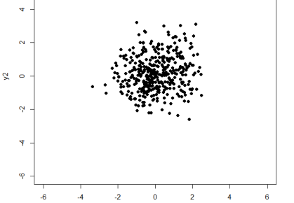
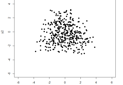
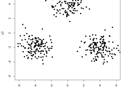
Figure 1: Variance decomposition of a mixture distribution. Scatter plots of samples from a standard normal mixture distribution with three components and equal weights, with a varying amount of heterogeneity $\phi_{B}$ explained by the variation of the component means, $\phi_{B}=0.1$, $\phi_{B}=0.5$ and $\phi_{B}=0.9$ (from left to right).

Regarding the prior specification of the subcomponent means $\boldsymbol{\mu}_{k1},\ldots,\boldsymbol{\mu}_{kL}$, we select the scale matrix $\mathbf{B}_{0}$ in order to concentrate a lot of mass near the cluster center $\mathbf{b}_{0k}$, pulling $\boldsymbol{\mu}_{kl}$ toward $\mathbf{b}_{0k}$. Matching the a priori expectation of the second term in the variance decomposition (10), given by

$$E\left(\sum_{k=1}^{K}\eta_{k}\left(\sum_{l=1}^{L}w_{kl}\boldsymbol{\mu}_{kl}\boldsymbol{\mu}_{kl}^{\prime}-{\boldsymbol{\mu}}_{k}{\boldsymbol{\mu}}_{k}^{\prime}\right)\right)=\sum_{k=1}^{K}E(\eta_{k})\sum_{l=1}^{L}E(w_{kl})E(\boldsymbol{\mu}_{kl}\boldsymbol{\mu}_{kl}^{\prime}-{\boldsymbol{\mu}}_{k}{\boldsymbol{\mu}}_{k}^{\prime})=\mathbf{B}_{0},$$

to the desired proportion of explained heterogeneity and, using once more only the main diagonal of $\mathbf{S}_{y}$ we obtain $\mathbf{B}_{0}=\phi_{W}(1-\phi_{B})\text{diag}(\mathbf{S}_{y})$, which incorporates our idea that only a small proportion $\phi_{W}$ of the within-cluster variability should be explained by the variability of the subcomponent means.

After having chosen $\phi_{B}$ and $\phi_{W}$, basically the cluster structure and shape is a priori determined. However, in order to allow for more flexibility in capturing the unknown cluster shapes in the sense that within each cluster the amount of shrinkage of the subcomponent means $\boldsymbol{\mu}_{kl}$ toward the cluster center $\mathbf{b}_{0k}$ need not to be the same for all dimensions, for each cluster $k$ and each dimension $j$ additionally a random adaptation factor $\lambda_{kj}$ is introduced in (8) which adjusts $\mathbf{B}_{0}$. The gamma prior for $\lambda_{kj}$ in (7) implies that the prior expectation of the covariance matrix of $\boldsymbol{\mu}_{kl}$ equals $\mathbf{B}_{0}$. However, $\lambda_{kj}$ acts as a local adjustment factor for cluster $k$ which allows to shrink (or inflate) the variance of subcomponent means $\mu_{klj}$ in dimension $j$ in order to adapt to a more (or less) dense cluster distribution as specified by $\mathbf{B}_{0}$. In order to allow only for small adjustments of the specified $\mathbf{B}_{0}$, we choose $\nu=10$, in this way almost 90% of the a priori values of $\lambda_{kj}$ are between $0.5$ and $1.5$. This hierarchical prior specification for $\boldsymbol{\mu}_{kl}$ corresponds to the normal gamma prior (Griffin and Brown, 2010) which has been applied by Frühwirth-Schnatter (2011) and Malsiner-Walli et al. (2016) in the context of finite mixture models for variable selection.

2.4 Relation to BNP mixtures

Our approach bears resemblance to various approaches in BNP modeling. First of all, the concept of sparse finite mixtures as used in Malsiner-Walli et al. (2016) is related to Dirichlet process (DP) mixtures (Müller and Mitra, 2013) where the discrete mixing distribution in the finite mixture (1) is substituted by a random distribution $G\sim DP(\alpha,H)$, drawn from a DP prior with precision parameter $\alpha$ and base measure $H$. As a draw $G$ from a DP is almost surely discrete, the corresponding model has a representation as an infinite mixture:

$$p(\mathbf{y}) =\sum\limits_{k=1}^{\infty}\eta_{k}p_{k}(\mathbf{y}|\boldsymbol{\theta}_{k}),$$ (13)

with i.i.d. atoms $\boldsymbol{\theta}_{k}\overset{iid}{\sim}H$ drawn from the base measure $H$ and weights $\eta_{k}=v_{k}\prod_{j=1}^{k-1}(1-v_{j})$ obeying the stick breaking representation with $v_{k}\overset{iid}{\sim}\mathcal{B}\left(1,\alpha\right)$ (Sethuraman, 1994).

If the hyperparameter in the weight distribution $\boldsymbol{\eta}$ of a sparse finite mixture is chosen as $e_{0}=\alpha/K$, i.e. $\boldsymbol{\eta}\sim Dir_{K}(\alpha/K)$, and the component parameters $\boldsymbol{\theta}_{k}\overset{iid}{\sim}H$ are i.i.d. draws from $H$, then as $K$ increases, the sparse finite mixture in Equation (1) converges to a DP mixture with mixing distribution $G\sim DP(\alpha,H)$, see Green and Richardson (2001). For example, the sparse finite Gaussian mixture introduced in Malsiner-Walli et al. (2016) converges to a Dirichlet process Gaussian mixture as $K$ increases, with $(\boldsymbol{\mu}_{k},\boldsymbol{\Sigma}_{k})$ being i.i.d. draws from the appropriate base measure $H$.

The more general sparse finite mixture of mixtures model introduced in this paper also converges to a Dirichlet process mixture where the atoms are finite mixtures indexed by the parameter $\boldsymbol{\theta}_{k}$ defined in (3). The parameters $\boldsymbol{\theta}_{k}$ are i.i.d. draws from the base measure (6), with strong dependence among the means $\boldsymbol{\mu}_{k1},\ldots,\boldsymbol{\mu}_{kL}$ and covariances $\boldsymbol{\Sigma}_{k1},\ldots,\boldsymbol{\Sigma}_{kL}$ within each cluster $k$. This dependence is achieved through the two-layer hierarchical prior described in (7) and (8) and is essential to create well-connected clusters from the subcomponents, as outlined in Section 2.3.

Also in the BNP framework models have been introduced that create dependence, either in the atoms and/or in the weights attached to the atoms. For instance, the nested DP process of Rodriguez et al. (2008) allows to cluster distributions across $N$ units. Within each unit $i$, $i=1,\ldots,N$, repeated (univariate) measurements $y_{it},t=1,\ldots,N_{i}$ arise as independent realizations of a DP Gaussian mixture with random mixing distribution $G_{i}$. The $G_{i}$s are i.i.d. draws from a DP, in which the base measure is itself a Dirichlet process $DP(\beta,H)$, i.e. $G_{i}\overset{iid}{\sim}DP(\alpha,DP(\beta,H))$. Hence, two distributions $G_{i}$ and $G_{j}$ either share the same weights and atoms sampled from $H$, or the weights and atoms are entirely different. If only a single observation $y_{i}$ is available in each unit, i.e. $N_{i}=1$, then the nested DP is related to our model. In particular, it has a two-layer representation as in (1) and (2), however with both $K$ and $L$ being infinite. The nested DP can, in principal, be extended to multivariate observations $\mathbf{y}_{i}$. In this case, $p(\mathbf{y}_{i})$ takes the same form as in (13), with the same stick breaking representation for the cluster weights $\eta_{1},\eta_{2},\ldots$. On the lower level, each cluster distribution $p_{k}(\mathbf{y}_{i}|\boldsymbol{\theta}_{k})$ is a DP Gaussian mixture:

$$p_{k}(\mathbf{y}_{i}|\boldsymbol{\theta}_{k}) =\sum\limits_{l=1}^{\infty}w_{kl}f_{\mathcal{N}}(\mathbf{y}_{i}|\boldsymbol{\mu}_{kl},\boldsymbol{\Sigma}_{kl}),$$ (14)

where the component weights $w_{kl}$ are derived from the stick breaking representation $w_{kl}=u_{kl}\prod_{j=1}^{l-1}(1-u_{kj}),l=1,2,\ldots$ where $u_{kl}\overset{iid}{\sim}\mathcal{B}\left(1,\beta\right)$. For the nested DP, dependence is introduced only on the level of the weights and sticks, as the component parameters $\boldsymbol{\mu}_{kl},\boldsymbol{\Sigma}_{kl}\overset{iid}{\sim}H$ are i.i.d. draws from the base measure $H$. This lack of prior dependence among the atoms $(\boldsymbol{\mu}_{kl},\boldsymbol{\Sigma}_{kl})$ is likely to be an obstacle in a clustering context.

The BNP approach most closely related to our model is the infinite mixture of infinite Gaussian mixtures (I²GMM) model of Yerebakan et al. (2014) which also deals with clustering multivariate observations from non-Gaussian component densities. The I²GMM model has a two-layer hierarchical representation like the nested DP. On the top level, i.i.d. cluster specific locations $\mathbf{b}_{0k}$ and covariances $\boldsymbol{\Sigma}_{k}$ are drawn from a random distribution $G\sim DP(\alpha,H)$ arising from a DP prior with base measure $H$ being equal to the conjugate normal-inverse-Wishart distribution. A cluster specific DP is introduced on the lower level as for the nested DP; however, the I²GMM model is more flexible, as prior dependence is also introduced among the atoms belonging to the same cluster. More precisely, ${\mathbf{y}}_{i}\sim\mathcal{N}_{r}(\boldsymbol{\mu}_{i},\boldsymbol{\Sigma}_{k})$, with $\boldsymbol{\mu}_{i}\overset{iid}{\sim}G_{k}$, where $G_{k}\sim DP(\beta,H_{k})$ is a draw from a DP with cluster specific base measure $H_{k}=\mathcal{N}_{r}(\mathbf{b}_{0k},\boldsymbol{\Sigma}_{k}/\kappa_{1})$.

It is easy to show that the I²GMM model has an infinite two-layer representation as in (13) and (14), with exactly the same stick breaking representation. However, the I²GMM model has a constrained form on the lower level, with homoscedastic covariances $\boldsymbol{\Sigma}_{kl}\equiv\boldsymbol{\Sigma}_{k}$, whereas the locations $\boldsymbol{\mu}_{kl}$ scatter around the cluster centers $\mathbf{b}_{0k}$ as in our model:

$$(\mathbf{b}_{0k},\boldsymbol{\Sigma}_{k})\overset{iid}{\sim}H,\qquad\boldsymbol{\mu}_{kl}|\mathbf{b}_{0k},\boldsymbol{\Sigma}_{k}\overset{iid}{\sim}H_{k}.$$ (15)

In our sparse mixture of mixtures model, we found it useful to base the density estimator on heteroscedastic covariances $\boldsymbol{\Sigma}_{kl}$, to better accommodate the non-Gaussianity of the cluster densities with a fairly small number $L$ of subcomponents. It should be noted that our semi-parametric density estimator is allowed to display non-convex shapes, as illustrated in Figure C.2 in the Appendix. Nevertheless, we could have considered a mixture in (2) where $\boldsymbol{\Sigma}_{kl}\equiv\boldsymbol{\Sigma}_{k}$, with the same base measure for the atoms $(\boldsymbol{\mu}_{k1},\ldots,\boldsymbol{\mu}_{kL},\boldsymbol{\Sigma}_{k})$ as in (15). In this case, the relationship between our sparse finite mixture and the I²GMM model would become even more apparent: by choosing $e_{0}=\alpha/K$ and $d_{0}=\beta/L$ and letting $K$ and $L$ go to infinity, our model would converge to the I²GMM model.

3 Clustering and posterior inference

3.1 Clustering and selecting the number of clusters

For posterior inference, two sequences of allocation variables are introduced, namely the cluster assignment indicators $\mathbf{S}=(S_{1},\ldots,S_{N})$ and the within-cluster allocation variables $\mathbf{I}=(I_{1},\ldots,I_{N})$. More specifically, $S_{i}\in\{1,\ldots,K\}$ assigns each observation $\mathbf{y}_{i}$ to cluster $S_{i}$ on the upper level of the mixture of mixtures model. On the lower level, $I_{i}\in\{1,\ldots,L\}$ assigns observation $\mathbf{y}_{i}$ to subcomponent $I_{i}$. Hence, the pair $(S_{i},I_{i})$ carries all the information needed to assign each observation to a unique component in the expanded mixture (4).

Note that for all observations ${\mathbf{y}}_{i}$ and ${\mathbf{y}}_{j}$ belonging to the same cluster, the upper level indicators $S_{i}=S_{j}$ will be the same, while the lower level indicators $I_{i}\neq I_{j}$ might be different, meaning that they belong to different subcomponents within the same cluster. It should be noted that the Dirichlet prior $\mathbf{w}_{k}\sim Dir_{L}(d_{0})$, with $d_{0}>d/2$, on the weight distribution ensures overlapping densities within each cluster, in particular if $L$ is overfitting. Hence the indicators $I_{i}$ will typically cover all possible values $\{1,\ldots,L\}$ within each cluster.

For clustering, only the upper level indicators $\mathbf{S}$ are explored, integrating implicitly over the uncertainty of assignment to the subcomponents on the lower level. A cluster $C_{k}=\{i|S_{i}=k\}$ is thus a subset of the data indices $\{1,\ldots,N\}$, containing all observations with identical upper level indicators. Hence, the indicators $\mathbf{S}$ define a random partition ${\cal P}=\{C_{1},\ldots,C_{K_{0}}\}$ of the $N$ data points in the sense of Lau and Green (2007), as $\mathbf{y}_{i}$ and $\mathbf{y}_{j}$ belong to the same cluster, if and only if $S_{i}=S_{j}$. The partition ${\cal P}$ contains $K_{0}=|{\cal P}|$ clusters, where $|{\cal P}|$ is the cardinality of ${\cal P}$. Due to the Dirichlet prior $\boldsymbol{\eta}\sim Dir_{K}(e_{0})$, with $e_{0}$ close to 0 to obtain a sparse finite mixture, $K_{0}$ is a random number being a priori much smaller than $K$.

For a sparse finite mixture model with $K$ clusters, the prior distribution over all random partitions ${\cal P}$ of $N$ observations is derived from the joint (marginal) prior $p({\mathbf{S}})=\int\prod_{i=1}^{N}p(S_{i}|{\boldsymbol{\eta}})d\,{\boldsymbol{\eta}}$ which is given, e.g., in Frühwirth-Schnatter (2006, p. 66):

$$\displaystyle p({\mathbf{S}})=\frac{\Gamma(Ke_{0})}{\Gamma(N+Ke_{0})\Gamma(e_{0})^{K_{0}}}\prod_{k:N_{k}>0}\Gamma(N_{k}+e_{0}),$$ (16)

where $N_{k}=\#\{S_{i}=k\}$. For a given partition ${\cal P}$ with $K_{0}$ data clusters, there are $K!/(K-K_{0})!$ assignment vectors ${\mathbf{S}}$ that belong to the equivalence class defined by ${\cal P}$. The prior distribution over all random partitions ${\cal P}$ is then obtained by summing over all assignment vectors ${\mathbf{S}}$ that belong to the equivalence class defined by ${\cal P}$:

$$\displaystyle p({\cal P}|K_{0})=\frac{K!}{(K-K_{0})!}\frac{\Gamma(Ke_{0})}{\Gamma(N+Ke_{0})\Gamma(e_{0})^{K_{0}}}\prod_{k:N_{k}>0}\Gamma(N_{k}+e_{0}),$$ (17)

which takes the form of a product partition model and therefore is invariant to permuting the cluster labels. Hence, it is possible to derive the prior predictive distribution $p(S_{i}|{\mathbf{S}}_{-i})$, where ${\mathbf{S}}_{-i}$ denote all indicators, excluding $S_{i}$. Let $K_{0}^{-i}$ be the number of non-empty clusters implied by ${\mathbf{S}}_{-i}$ and let $N_{k}^{-i}$ be the corresponding cluster sizes. From (16), we obtain the following probability that $S_{i}$ is assigned to an existing cluster $k$:

$$\displaystyle\mbox{\rm Pr}\{S_{i}=k|{\mathbf{S}}_{-i},N_{k}^{-i}>0\}=\frac{N_{k}^{-i}+e_{0}}{N-1+e_{0}K}.$$ (18)

The prior probability that $S_{i}$ creates a new cluster with $S_{i}\in I=\{k|N_{k}^{-i}=0\}$ is equal to

$$\displaystyle\mbox{\rm Pr}\{S_{i}\in I|{\mathbf{S}}_{-i}\}=(K-K_{0}^{-i})\mbox{\rm Pr}\{S_{i}=k^{*}|{\mathbf{S}}_{-i},k^{*}\in I\}=\frac{e_{0}(K-K_{0}^{-i})}{N-1+e_{0}K}.$$ (19)

It is illuminating to investigate the prior probability to create new clusters in detail. First of all, for $e_{0}$ independent of $K$, this probability not only depends on $e_{0}$, but also increases with $K$. Hence a sparse finite mixture model based on the prior ${\boldsymbol{\eta}}\sim\mathcal{D}_{K}\left(e_{0}\right)$ can be regarded as a two-parameter model, where both $e_{0}$ and $K$ influence the a priori expected number of data clusters $K_{0}$ which is determined for a DP mixture solely by $\alpha$. A BNP two-parameter mixture is obtained from the Pitman-Yor process (PYP) prior $PY{(\beta,\alpha)}$ with $\beta\in[0,1),\alpha>-\beta$ (Pitman and Yor, 1997), with stickbreaking representation $v_{k}\overset{iid}{\sim}\mathcal{B}\left(1-\beta,\alpha+k\beta\right)$. The DP prior results as that special case where $\beta=0$.

Second, the prior probability (19) to create new clusters in a sparse finite mixture model decreases, as the number $K_{0}^{-i}$ of non-empty clusters increases. This is in sharp contrast to DP mixtures where this probability is constant and PYP mixtures where this probability increases, see e.g., Fall and Barat (2014).

Finally, what distinguishes a sparse finite mixture model, both from a DP as well as a PYP mixture, is the a priori expected number of data clusters $K_{0}$, as the number $N$ of observations increases. For $K$ and $e_{0}$ independent of $N$, the probability to create new clusters decreases, as $N$ increases, and converges to 0, as $N$ goes to infinity. Therefore, $K_{0}$ is asymptotically independent of $N$ for sparse finite mixtures, whereas for the DP process $K_{0}\sim\alpha\log(N)$ (Korwar and Hollander, 1973) and $K_{0}\sim N^{\beta}$ obeys a power law for PYP mixtures (Fall and Barat, 2014). This leads to quite different clustering behavior for these three types of mixtures.

A well-known limitation of DP priors is that a priori the cluster sizes are expected to be geometrically ordered, with one big cluster, geometrically smaller clusters, and many singleton clusters (Müller and Mitra, 2013). PYP mixtures are known to be more useful than the DP mixture for data with many significant, but small clusters. A common criticism concerning finite mixtures is that the number of clusters needs to be known a priori. Since this is not the case for sparse finite mixtures, they are useful in the context of clustering, in particular in cases where the data arise from a moderate number of clusters, that does not increase as the number of data points $N$ increases.

3.2 MCMC estimation and posterior inference

Bayesian estimation of the sparse hierarchical mixture of mixtures model is performed using MCMC methods based on data augmentation and Gibbs sampling. We only need standard Gibbs sampling steps, see the detailed MCMC sampling scheme in Appendix A.

In order to perform inference based on the MCMC draws, i.e. to cluster the data, to estimate the number of clusters, to solve the label switching problem on the higher level and to estimate cluster-specific parameters, several existing procedures can be easily adapted and applied to post-process the posterior draws of a mixture of mixtures model, e.g., those which are, for instance, implemented in the R packages PReMiuM (Liverani et al., 2015) and label.switching (Papastamoulis, 2015).

For instance, the approach in PReMiuM is based on the posterior probabilities of co-clustering, expressed through the similarity matrix $\mbox{\rm Pr}\{S_{i}=S_{j}|{\mathbf{y}}\}$ which can be estimated from the $M$ posterior draws $\mathbf{S}^{(m)},m=1,\ldots,M$, see Appendix B for details. The methods implemented in label.switching aim at resolving the label switching problem when fitting a finite mixture model using Bayesian estimation. Note that in the case of the mixture of mixtures model label switching occurs on two levels. On the cluster level, the label switching problem is caused by invariance of the mixture likelihood given in Equation (1) with respect to reordering of the clusters. On this level, label switching has to be resolved, since the single cluster distributions need to be identified. On the subcomponent level, label switching happens due to the invariance of Equation (2) with respect to reordering of the subcomponents. As we are only interested in estimating the entire cluster distributions, it is not necessary to identify the single subcomponents. Therefore, the label switching problem can be ignored on this level.

In this paper, the post-processing approach employed first performs a model selection step. The posterior draws of the indicators $\mathbf{S}^{(m)},m=1,\ldots,M$ are used to infer the number of non-empty clusters $K_{0}^{(m)}$ on the upper level of the mixture of mixtures model and the number of data clusters is then estimated as the mode. Conditional on the selected model, an identified model is obtained based on the point process representation of the estimated mixture. This method was introduced in Frühwirth-Schnatter (2006, p. 96) and successfully applied to model-based clustering in various applied research, see e.g. Frühwirth-Schnatter (2011) for some review. This procedure has been adapted to sparse finite mixtures in Frühwirth-Schnatter (2011) and Malsiner-Walli et al. (2016) and is easily extended to deal with sparse mixture of mixtures models, see Appendix B for more details. We will use this post-processing approach in our simulation studies and the applications in Section 4 and Appendices C, D and F to determine a partition of the data based on the maximum a posteriori (MAP) estimates of the relabeled cluster assignments.

4 Simulation studies and applications

The performance of the proposed strategy for selecting the unknown number of clusters and identifying the cluster distributions is illustrated in two simulation studies. In the first simulation study we investigate whether we are able to capture dense non-Gaussian data clusters and estimate the true number of data clusters. Furthermore, the influence of the specified maximum number of clusters $K$ and subcomponents $L$ on the clustering results is studied. In the second simulation study the sensitivity of the a priori defined proportions $\phi_{B}$ and $\phi_{W}$ on the clustering result is investigated. For a detailed description of the simulation design and results see Appendix C. Overall, the results indicated that our approach performed well and yielded promising results.

To further evaluate our approach, we fit the sparse hierarchical mixture of mixtures model on benchmark data sets and real data. First, we consider five data sets which were previously used to benchmark algorithms in cluster analysis. For these data sets we additionally apply the “merging strategy” proposed by Baudry et al. (2010) in order to compare the results to those of our approach. For these benchmark data sets class labels are available and we assess the performance by comparing how well our approach is able to predict the class labels using the cluster assignments, measured by the misclassification rate as well as the adjusted Rand index.

To assess how the algorithm scales to larger data sets we investigate the application to two flow cytometry data sets. The three-dimensional DLBCL data set (Lee and McLachlan, 2013b) consists of around 8000 observations and comes with manual class labels which can be used as benchmark. The GvHD data set (Brinkman et al., 2007) consists of 12441 observations, but no class labels are available. We compare the clusters detected for this data set qualitatively to solutions previously reported in the literature.

The detailed description of all investigated data sets as well as of the derivation of the performance measures are given in Appendix D. For the benchmark data sets, the number of estimated clusters $\hat{K}_{0}$, the adjusted Rand index ($\mathit{adj}$), and misclassification rate ($\mathit{er}$) are reported in Table 1 for all estimated models. In the first columns of Table 1, the name of the data set, the number of observations $N$, the number of variables $r$ and the number of true classes $K^{true}$ (if known) are reported. To compare our approach to the merging approach proposed by Baudry et al. (2010), we use the function Mclust of the R package mclust (Fraley et al., 2012) to first fit a standard normal mixture distribution with the maximum number of components $K=10$. The number of estimated normal components based on the BIC is reported in the column Mclust. Then the selected components are combined hierarchically to clusters by calling function clustCombi from the same package (column clustCombi). The number of clusters is chosen by visual detection of the change point in the plot of the rescaled differences between successive entropy values, as suggested by Baudry et al. (2010). Furthermore, to compare our results to those obtained if a cluster distribution is modeled by a single normal distribution only, a sparse finite mixture model with $K=10$ (Malsiner-Walli et al., 2016) is fitted to the data sets (column SparseMix). The results of fitting a sparse hierarchical mixture of mixtures model with $K=10$ are given in column SparseMixMix, where $L=5$ is compared to our default choice of $L=4$ to investigate robustness with respect to the choice of $L$. For each estimation, MCMC sampling is run for 4000 iterations after a burn-in of 4000 iterations.

As can be seen in Table 1, for all data sets the sparse hierarchical mixture of mixtures model is able to capture the data clusters quite well both in terms of the estimated number of clusters and the clustering quality measured by the misclassification rate as well as the adjusted Rand index. In general, our approach is not only outperforming the standard model-based clustering model using mixtures of Gaussians regarding both measures, but also the approach proposed by Baudry et al. (2010). In addition, it can be noted that for all data sets the estimation results remain quite stable, if the number of subcomponents $L$ is increased to $5$, see the last column in Table 1. The results for the Yeast data set are of particular interest as they indicate that clustCombi completely fails. Although the misclassification rate of 25% implies that only a quarter of the observations is assigned to “wrong” clusters, inspection of the clustering obtained reveals that almost all observations are lumped together in a single, very large cluster, whereas the few remaining observations are split into five very small clusters. This bad clustering quality is better reflected by the adjusted Rand index which takes a negative value ($\mathit{adj}=-0.02$), i.e. is “worse than would be expected by guessing” (Franczak et al., 2012). For the flower data set, more results are given in Appendix D where the obtained clustering and cluster distributions are illustrated.

				Mclust		SparseMix	SparseMixMix
				$K=10$		$K=10$	$K=10$
Data set	$N$	$r$	$K^{true}$	Mclust	clustCombi	$L=1$	$L=4$	$L=5$
Yeast	626	3	2	$8$ (.50, .20)	$6$ (-.02, 0.25)	$6$ (.48, .23)	$\mathbf{2}$ (.68, .08)	$2$ (.71, .07)
Flea beetles1	74	6	3	$5$ (.77, .18)	$4$ (.97, .03)	$3$ (1.00, .00)	$\mathbf{3}$ (1.00, .00)	$3$ (1, .00)
AIS	202	3	2	$3$ (.73, .13)	$2$ (.66, .09)	$3$ (.76, .11)	$\mathbf{2}$ (.81, .05)	$2$ (.76, .06)
Wisconsin	569	3	2	$4$ (.55, .30)	$4$ (.55, .30)	$4$ (.62, .21)	$\mathbf{2}$ (.82, .05)	$2$ (.82, .05)
Flower	400	2	4	$6$ (.52, .35)	$4$ (.99, .01)	$5$ (.67, .20)	$\mathbf{4}$ (.97, .01)	$4$ (.97, .02)

Table 1: Results for the estimated number of data clusters $\hat{K}_{0}$ for various benchmark data sets, using the functions Mclust to fit a standard mixture model with $K=10$ and clustCombi to estimate a mixture with combined components (column Mclust), using a sparse finite mixture model with $K=10$ (column SparseMix), and estimating a sparse hierarchical mixture of mixtures model with $K=10$, $\phi_{B}=0.5$ and $\phi_{W}=0.1$, and $L=4,5$ (column SparseMixMix). Priors and hyperparameter specifications are selected as described in Section 2. In parentheses, the adjusted Rand index (“1” corresponds to perfect classification) and the proportion of misclassified observations (“0” corresponds to perfect classification) are reported.

In order to investigate the performance of our approach on larger data sets with a slightly different cluster structure, we fit the sparse hierarchical mixture of mixtures model to two flow cytometry data sets. These applications also allow us to indicate how the prior settings need to be adapted if a different cluster structure is assumed to be present in the data. As generally known, flow cytometry data exhibit non-Gaussian characteristics such as skewness, multimodality and a large number of outliers, as can be seen in the scatter plot of two variables of the GvHD data set in Figure 3. Thus, we specified a sparse hierarchical mixture of mixtures model with $K=30$ clusters and increased the number of subcomponents forming a cluster to $L=15$ in order to handle more complex shapes of the cluster distributions given the large amount of data. Since the flow cytometry data clusters have a lot of outliers similar to the clusters generated by shifted asymmetric Laplace ($\mathit{SAL}$) distributions (see Appendix F), we substitute the hyperprior $\mathbf{C}_{0k}\sim\mathcal{W}_{r}(g_{0},\mathbf{G}_{0})$ by the fixed value $\mathbf{C}_{0k}=g_{0}\mathbf{G}_{0}^{-1}$ and set $\lambda_{kj}\equiv 1$, $j=1,\ldots,r$ to prevent that within a cluster the subcomponent covariance matrices are overly shrunken and become too similar. In this way, subcomponent covariance matrices are allowed to vary considerably within a cluster and capture both a dense cluster region around the cluster center and scattered regions at the boundary of the cluster.

We fit this sparse hierarchical mixture of mixtures model to the DLBCL data after removing 251 dead cells. For most MCMC runs after a few hundred iterations all but four clusters become empty during MCMC sampling. The estimated four cluster solution coincides almost exactly with the cluster solution obtained with manual gating; the adjusted Rand index is 0.95 and the error rate equals 0.03. This error rate outperforms the error rate of 0.056 reported by Lee and McLachlan (2013b). In Figure 2 the estimated four cluster solution is visualized.

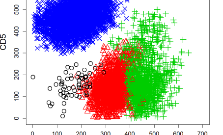
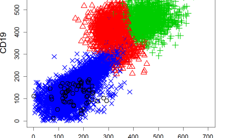
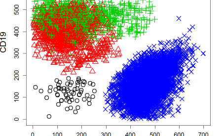
Figure 2: Flow cytometry data set DLBCL. Scatterplot of the clustering results.

When fitting a sparse hierarchical mixture of mixtures model to the GvHD data, the classifications resulting from different runs of the MCMC algorithm seemed to be rather stable. The obtained solutions differ mainly in the size of the two large clusters with low expressions. These, however, are supposed to not contain any information regarding the development of the disease. On the right hand side of Figure 3, the results of one specific run are shown in a heatmap. In this run, we found eight clusters which are similar to those reported by Frühwirth-Schnatter and Pyne (2010) when fitting a skew-$t$ mixture model to these data. In the heatmap each row represents the location of a six-dimensional cluster, and each column represents a particular marker (variable). The red, white and blue colors denote high, medium and low expressions.

As in Frühwirth-Schnatter and Pyne (2010), we identified two larger clusters (43% and 20.4%, first two rows in the heatmap) with rather low expressions in the last four variables. We also identified a smaller cluster (3.8%, forth row from the bottom) representing live cells (high values in the first two variables) with a unique signature in the other four variables (high values in all four variables). Also two other small clusters can be identified (second and third row from the bottom) which have a signature very similar to the clusters found by Frühwirth-Schnatter and Pyne (2010), and thus our results confirm their findings.

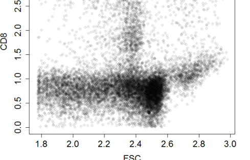
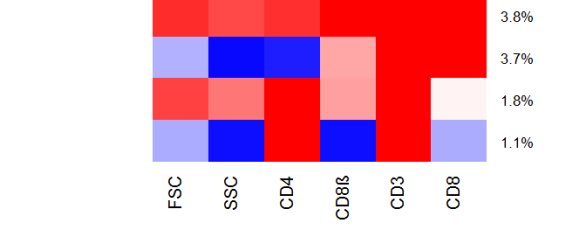
Figure 3: Flow cytometry data set GvHD. Scatter plot of two variables (“FSC”, “CD8”) (left-hand side), and heatmap of the clustering results by fitting a sparse hierarchical mixture of mixtures model (right-hand side). In the heatmap, each row represents the location of a six-dimensional cluster, and each column represents a particular marker. The red, white and blue colors denote high, medium and low expression, respectively.

5 Discussion

We propose suitable priors for fitting an identified mixture of normal mixtures model within the Bayesian framework of model-based clustering. This approach allows for (1) automatic determination of the number of clusters and (2) semi-parametric approximation of non-Gaussian cluster distributions by mixtures of normals. We only require the assumption that the cluster distributions are dense and connected. Our approach consists in the specification of structured informative priors on all model parameters. This imposes a rigid hierarchical structure on the normal subcomponents and allows for simultaneous estimation of the number of clusters and their approximating distributions. This is in contrast to the two-step merging approaches, where in the first step the data distribution is approximated by a suitable normal mixture model. However, because this approximation is made without taking the data clusters into account which are reconstructed only in the second step of the procedure, the general cluster structure might be missed by these approaches.

As we noted in our simulation studies, the way in which the cluster mixture distributions are modeled by the subcomponent densities is crucial for the clustering result. Enforcing overlapping subcomponent densities is essential in order to avoid that a single subcomponent becomes too narrow thus leading to a small a posteriori cluster probability for observations from this subcomponent. Also, enforcing that observations are assigned to all subcomponents during MCMC sampling is important as the estimation of empty subcomponents would bias the resulting cluster distribution because of the “prior” subcomponents. For modeling large, overlapping subcomponent densities, crucial model parameters are the a priori specified covariance matrix of the subcomponent means and the scale matrix of the inverse Wishart prior for the subcomponent covariance matrices. We select both crucial hyperparameters based on the variance decomposition of a mixture of mixtures model.

We found a prior setting which is able to capture dense and connected data clusters in a range of benchmark data sets. However, if interest lies in detection of different cluster shapes, a different tuning of the prior parameters may be required. Therefore, it would be interesting to investigate in more detail how we can use certain prior settings to estimate certain kinds of data clusters. Then it would be possible to give recommendations which prior settings have to be used in order to capture certain types of data clusters. For instance, mixtures of shifted asymmetric Laplace ($\mathit{SAL}$) distributions, introduced by Franczak et al. (2012), have cluster distributions which are non-dense and have a strongly asymmetric shape with comet-like tails. In this case, the prior specifications given in Section 2 are not able to capture the clusters and need to be tuned to capture also this special kind of data clusters, see the example given in Appendix F.

Although our approach to estimate the number of clusters worked well for many data sets, we encountered mixing problems with the blocked conditional Gibbs sampler outlined in Appendix A, in particular in high dimensional spaces with large data sets. To alleviate this problem, a collapsed sampler similar to Fall and Barat (2014) could be derived for finite mixtures. However, we leave this for future research.

SUPPLEMENTARY MATERIAL

Appendix containing (A) the MCMC scheme to estimate a mixture of mixtures model, (B) a detailed description of the post-processing strategy based on the point process representation, (C) the simulation studies described in Section 4, (D) a description of the data sets studied in Section 4, (E) issues with the merging approach, and (F) estimation of data clusters generated by a $SAL$-distribution (Franczak et al., 2012). (Appendix.pdf)

R code implementing the sparse hierarchical mixture of mixtures model (Code.zip).

Appendix A MCMC sampling scheme

Estimation of a sparse hierarchical mixture of mixtures model is performed through MCMC sampling based on data augmentation and Gibbs sampling. To indicate the cluster to which each observation belongs, latent allocation variables $\mathbf{S}=(S_{1},\ldots,S_{N})$ taking values in $\{1,\ldots,K\}^{N}$ are introduced such that

$$p(\mathbf{y}_{i}|\boldsymbol{\theta}_{1},\ldots,\boldsymbol{\theta}_{K},S_{i}=k)=p_{k}(\mathbf{y}_{i}|\boldsymbol{\theta}_{k}),\quad\text{ and }\quad\mbox{\rm Pr}\{S_{i}=k|\boldsymbol{\eta}\}=\eta_{k}.$$

Additionally, to indicate the subcomponent to which an observation within a cluster is assigned to, latent allocation variables $\mathbf{I}=(I_{1},\ldots,I_{N})$ taking values in $\{1,\ldots,L\}^{N}$ are introduced such that

$$p_{k}(\mathbf{y}_{i}|\boldsymbol{\theta}_{k},S_{i}=k,I_{i}=l)=f_{\mathcal{N}}(\mathbf{y}_{i}|\boldsymbol{\mu}_{kl},\boldsymbol{\Sigma}_{kl})\quad\text{ and }\quad\mbox{\rm Pr}\{I_{i}=l|S_{i}=k,\mathbf{w}_{k}\}=w_{kl}.$$

Based on the priors specified in Section 2.2, with fixed hyperparameters $(e_{0},d_{0},c_{0},g_{0},\mathbf{G}_{0},\mathbf{B}_{0},\mathbf{m}_{0},\mathbf{M}_{0},\nu)$, the latent variables $(\mathbf{S},\mathbf{I})$ and parameters $(\boldsymbol{\eta},\mathbf{w}_{k},\boldsymbol{\mu}_{kl},\boldsymbol{\Sigma}_{kl},$ $\mathbf{C}_{0k},$ $\mathbf{b}_{0k},$ $\lambda_{kj})$, $k=1,\dots,K$, $l=1,\ldots,L$, $j=1,\ldots,r$, are sampled from the posterior distribution using the following Gibbs sampling scheme. Note that the conditional distributions given do not indicate that conditioning is also on the fixed hyperparameters.

1. Sampling steps on the level of the cluster distribution:

   1. Parameter simulation step conditional on the classifications $\mathbf{S}$. Sample $\boldsymbol{\eta}|\mathbf{S}$ from $Dir(e_{1},\ldots,e_{K})$, $e_{k}=e_{0}+N_{k}$, $k=1,\dots,K$, where $N_{k}=\#\{S_{i}|S_{i}=k\}$ is the number of observations allocated to cluster $k$.

   2. Classification step for each observation $\mathbf{y}_{i}$ conditional on cluster-specific parameters. For each $i=1,\ldots,N$ sample the cluster assignment $S_{i}$ from

      $$\mbox{\rm Pr}\{S_{i}=k|\mathbf{y}_{i},\boldsymbol{\theta},\boldsymbol{\eta}\} \propto\eta_{k}p_{k}(\mathbf{y}_{i}|\boldsymbol{\theta}_{k}),\;k=1,\ldots,K,$$ (20)

      where $p_{k}(\mathbf{y}_{i}|\boldsymbol{\theta}_{k})$ is the semi-parametric mixture approximation of the cluster density:

      $$p_{k}(\mathbf{y}_{i}|\boldsymbol{\theta}_{k}) =\sum_{l=1}^{L}w_{kl}f_{\mathcal{N}}(\mathbf{y}_{i}|\boldsymbol{\mu}_{kl},\boldsymbol{\Sigma}_{kl}).$$

      Note that clustering of the observations is performed on the upper level of the model, using a collapsed Gibbs step, where the latent, within-cluster allocation variables $\mathbf{I}$ are integrated out.

2. Within each cluster $k$, $k=1,\ldots,K$:

   1. Classification step for all observations $\mathbf{y}_{i}$, assigned to cluster $k$ (i.e. $S_{i}=k$), conditional on the subcomponent weights and the subcomponent-specific parameters. For each $i\in\{i=1,\ldots,N:S_{i}=k\}$ sample $I_{i}$ from

      $$\mbox{\rm Pr}\{I_{i}=l|\mathbf{y}_{i},\boldsymbol{\theta}_{k},S_{i}=k\}\propto w_{kl}f_{\mathcal{N}}(\mathbf{y}_{i}|\boldsymbol{\mu}_{kl},\boldsymbol{\Sigma}_{kl}),\;l=1,\ldots,L.$$

   2. Parameter simulation step conditional on the classifications $\mathbf{I}$ and $\mathbf{S}$:

      1. Sample $\mathbf{w}_{k}|\mathbf{I},\mathbf{S}$ from $Dir(d_{k1},\ldots,d_{kL})$, $d_{kl}=d_{0}+N_{kl}$, $l=1,\ldots,L$, where $N_{kl}=\#\{I_{i}=l|S_{i}=k\}$ is the number of observations allocated to subcomponent $l$ in cluster $k$.

      2. For $l=1,\ldots,L$: Sample $\boldsymbol{\Sigma}_{kl}^{-1}|\mathbf{S},\mathbf{I},\boldsymbol{\mu}_{kl},\mathbf{C}_{0k},\mathbf{y}\sim\mathcal{W}_{r}(c_{kl},\mathbf{C}_{kl})$, where

         $$c_{kl} =c_{0}+N_{kl}/2,$$

         $$\mathbf{C}_{kl} =\mathbf{C}_{0k}+\frac{1}{2}\sum\limits_{i:I_{i}=l,S_{i}=k}(\mathbf{y}_{i}-\boldsymbol{\mu}_{kl})(\mathbf{y}_{i}-\boldsymbol{\mu}_{kl})^{\prime}.$$

      3. For $l=1,\ldots,L$: Sample $\boldsymbol{\mu}_{kl}|\mathbf{S},\mathbf{I},\mathbf{b}_{0k},\boldsymbol{\Sigma}_{kl},\boldsymbol{\Lambda}_{k},\mathbf{y}\sim\mathcal{N}_{r}(\mathbf{b}_{kl},\mathbf{B}_{kl})$, where

         $$\mathbf{B}_{kl} =(\tilde{\mathbf{B}}_{0k}^{-1}+N_{kl}\boldsymbol{\Sigma}_{kl}^{-1})^{-1},$$

         $$\mathbf{b}_{kl} =\mathbf{B}_{kl}(\tilde{\mathbf{B}}_{0k}^{-1}\mathbf{b}_{0k}+\boldsymbol{\Sigma}_{kl}^{-1}N_{kl}\bar{\mathbf{y}}_{kl}),$$

         with $\tilde{\mathbf{B}}_{0k}=\sqrt{\boldsymbol{\Lambda}_{k}}\mathbf{B}_{0}\sqrt{\boldsymbol{\Lambda}_{k}}$, $\boldsymbol{\Lambda}_{k}=\text{diag}(\lambda_{k1},\ldots,\lambda_{kr}),$ and $\bar{\mathbf{y}}_{kl}=1/N_{kl}\sum\limits_{i:I_{i}=l,S_{i}=k}\mathbf{y}_{i}$ being equal to the subcomponent mean for $N_{kl}>0$ and $N_{kl}\bar{\mathbf{y}}_{kl}=0$, otherwise.

3. For each cluster $k$, $k=1,\ldots,K$: Sample the random hyperparameters $\lambda_{kj}$, $\mathbf{C}_{0k},\mathbf{b}_{0k}$ from their full conditionals:

   1. For $j=1,\ldots,r$: Sample $\lambda_{kj}|\mathbf{b}_{0k},\boldsymbol{\mu}_{k1},\ldots,\boldsymbol{\mu}_{kL}\sim\mathcal{GIG}(p_{kL},a_{kj},b_{kj})$, where $\mathcal{GIG}$ is the generalized inverted Gaussian distribution and

      $$p_{kL} =-L/2+\nu,$$

      $$a_{kj} =2\nu,$$

      $$b_{kj} =\sum_{l=1}^{L}(\mu_{kl,j}-b_{0k,j})^{2}/B_{0,jj}.$$

   2. Sample $\mathbf{C}_{0k}|\boldsymbol{\Sigma}_{k1},\ldots,\boldsymbol{\Sigma}_{kL}\sim\mathcal{W}_{r}(g_{0}+Lc_{0},\mathbf{G}_{0}+\sum_{l=1}^{L}\boldsymbol{\Sigma}_{kl}^{-1})$.

   3. Sample $\mathbf{b}_{0k}|\tilde{\mathbf{B}}_{0k},\boldsymbol{\mu}_{k1},\ldots,\boldsymbol{\mu}_{kL}\sim\mathcal{N}_{r}(\tilde{\mathbf{m}}_{k},\tilde{\mathbf{M}}_{k})$, where

      $$\tilde{\mathbf{M}}_{k} =(\mathbf{M}_{0}^{-1}+L\tilde{\mathbf{B}}_{0k}^{-1})^{-1},$$

      $$\tilde{\mathbf{m}}_{k} =\tilde{\mathbf{M}}_{k}\left(\mathbf{M}_{0}^{-1}\mathbf{m}_{0}+\tilde{\mathbf{B}}_{0k}^{-1}\sum_{l=1}^{L}\boldsymbol{\mu}_{kl}\right).$$

Appendix B Identification through clustering in the point process representation

Various post-processing approaches have been proposed for the MCMC output of finite or infinite mixture models (see, for example, Molitor et al. 2010 or Jasra et al. 2005). We pursue an approach which aims at determining a unique labeling of the MCMC draws after selecting a suitable number of clusters in order to base any posterior inference on the relabeled draws, such as for example the determination of cluster assignments.

To obtain a unique labeling of the clusters, Frühwirth-Schnatter (2006) suggested to post-process the MCMC output by clustering a vector-valued functional $f(\boldsymbol{\theta}_{k})$ of the cluster-specific parameters $\boldsymbol{\theta}_{k}$ in the point process representation. The point process representation has the advantage that it allows to study the posterior distribution of cluster-specific parameters regardless of potential label switching, which makes it very useful for identification.

If the number $K$ of components matches the true number of clusters, it can be expected that the vector-valued functionals of the posterior draws cluster around the “true” points $\{f(\boldsymbol{\theta}_{1}),\ldots,f(\boldsymbol{\theta}_{K})\}$ (Frühwirth-Schnatter, 2006, p. 96). However, in the case of an overfitting mixture where draws are sampled from empty components, the clustering procedure has to be adapted as suggested in Frühwirth-Schnatter (2011) and described in more details in Malsiner-Walli et al. (2016). Subsequently, we describe how this approach can be applied to identify cluster-specific characteristics for the sparse hierarchical mixture of mixtures model.

First, we estimate the number of non-empty clusters $\hat{K}_{0}$ on the upper level of the sparse hierarchical mixture of mixtures model. For this purpose, during MCMC sampling for each iteration $m$ the number of non-empty clusters $K_{0}^{(m)}$ is determined, i.e. the number of clusters to which observations have been assigned for this particular sweep of the sampler:

$$K_{0}^{(m)}=K-\sum\limits_{k=1}^{K}I\{N_{k}^{(m)}=0\},$$ (21)

where $N_{k}^{(m)}=\sum_{i=1}^{N}I\{S_{i}^{(m)}=k\}$ is the number of observations allocated to cluster $k$ in the upper level of the mixture for iteration $m$ and $I$ denotes the indicator function. Then, following Nobile (2004) we obtain the posterior distribution of the number $K_{0}$ of non-empty clusters $\mbox{\rm Pr}\{K_{0}=h|\mathbf{y}\},h=1,\ldots,K,$ on the upper level from the MCMC output. An estimator of the true number of clusters $\hat{K}_{0}$ is then given by the value visited most often by the MCMC procedure, i.e. the mode of the (estimated) posterior distribution $\mbox{\rm Pr}\{K_{0}=h|\mathbf{y}\}$.

After having estimated the number of non-empty clusters $\hat{K}_{0}$, we condition the subsequent analysis on a model with $\hat{K}_{0}$ clusters by removing all draws generated in iterations where the number of non-empty clusters does not correspond to $\hat{K}_{0}$. Among the remaining $M_{0}$ draws, only the non-empty clusters are relevant. Hence, we remove all cluster-specific draws $\boldsymbol{\theta}_{k}$ for empty clusters (which have been sampled from the prior). The cluster-specific draws left are samples from $\hat{K}_{0}$ non-empty clusters and form the basis for clustering the vector-valued functionals of the draws in the point process representation into $\hat{K}_{0}$ groups.

It should be noted, that using only vector-valued functionals of the unique parameters $\boldsymbol{\theta}_{k}$ for this clustering procedure has two advantages. First, $\boldsymbol{\theta}_{k}$ is a fairly high-dimensional parameter of dimension $d=L-1+Lr(r+3)/2$, in particular if $r$ is large, and the vector-valued functional allows to consider a lower dimensional problem (see also Frühwirth-Schnatter, 2006, 2011). In addition, we need to solve the label switching issue only on the upper level of the sparse hierarchical mixture of mixtures model. Thus, we choose vector-valued functionals of the cluster-specific parameters $\boldsymbol{\theta}_{k}$ that are invariant to label switching on the lower level of the mixture for clustering in the point process representation of the upper level. We found it particularly useful to consider the cluster means on the upper level mixture, defined by $\boldsymbol{\mu}_{k}^{(m)}=\sum_{l=1}^{L}w_{kl}^{(m)}\boldsymbol{\mu}_{kl}^{(m)}$.

Clustering the cluster means in the point process representation results in a classification sequence $\rho^{(m)}$ for each MCMC iteration $m$ indicating to which class a single cluster-specific draw belongs. For this, any clustering algorithm could be used, e.g., $K$-means (Hartigan and Wong, 1979) or $K$-centroids cluster analysis (Leisch, 2006) where the distance between a point and a cluster is determined by the Mahalanobis distance, see Malsiner-Walli et al. (2016, Section 4.2) for more details. Only the classification sequences $\rho^{(m)}$ which correspond to permutations of $(1,\ldots,\hat{K}_{0})$ are used to relabel the draws. To illustrate this step, consider for instance, that for $\hat{K}_{0}=4$, for iteration $m$ a classification sequence $\rho^{(m)}=(1,3,4,2)$ is obtained through the clustering procedure. That means that the draw of the first cluster was assigned to class one, the draw of the second cluster was assigned to class three and so on. In this case, the draws of this iteration are assigned to different classes, which allows to relabel these draws. As already observed by Frühwirth-Schnatter (2006), all classification sequences $\rho^{(m)}$, $m=1,\ldots,M$ obtained in this step are expected to be permutations, if the point process representation of the MCMC draws contains well-separated simulation clusters.

Nevertheless, it might happen that some of the classification sequences $\rho^{(m)}$ are not permutations. E.g., if the classification sequence $\rho^{(m)}=(3,1,2,1)$ is obtained, then draws sampled from two different clusters are assigned to the same class and no unique labels can be assigned. If only a small fraction $M_{0,\rho}$ of non-permutations is present, then the posterior draws corresponding to the non-permutation sequences are removed from the $M_{0}$ draws with $\hat{K}_{0}$ non-empty clusters. For the remaining $M_{0}(1-M_{0,\rho})$ draws, a unique labeling is achieved by relabeling the clusters according to the classification sequences $\rho^{(m)}$. If the fraction $M_{0,\rho}$ is high, this indicates that in the point process representation clusters are overlapping. This typically happens if the selected mixture model with $\hat{K}_{0}$ clusters is overfitting, see Frühwirth-Schnatter (2011).

This post-processing strategy of the MCMC draws obtained using the sampling strategy described in Appendix A can be summarized as follows:

1. For each iteration $m=1,\ldots,M$ of the MCMC run, determine the number of non-empty clusters $K_{0}^{(m)}$ according to (21).

2. Estimate the number of non-empty clusters by $\hat{K}_{0}=mode(K_{0}^{(m)})$ as the value of the number of non-empty clusters occurring most often during MCMC sampling.

3. Consider only the subsequence of all MCMC iterations of length $M_{0}$ where the number of non-empty clusters $K_{0}^{(m)}$ is exactly equal to $\hat{K}_{0}$. For each of the resulting $m=1,\ldots,M_{0}$ draws, relabel the posteriors draws $\boldsymbol{\theta}_{1}^{(m)},\ldots,\boldsymbol{\theta}_{K}^{(m)}$, the weight distribution $\eta_{1}^{(m)},\ldots,\eta_{K}^{(m)}$, as well as the upper level classifications $S_{1}^{(m)},\ldots,S_{N}^{(m)}$ such that empty clusters, i.e. clusters with $N_{k}^{(m)}=0$, appear last. Remove the empty clusters and keep only the draws $\boldsymbol{\theta}_{1}^{(m)},\ldots,\boldsymbol{\theta}_{\hat{K}_{0}}^{(m)}$ of the $\hat{K}_{0}$ non-empty clusters.

4. Arrange the $\hat{K}_{0}$ cluster means $\boldsymbol{\mu}_{1}^{(m)},\ldots,\boldsymbol{\mu}_{\hat{K}_{0}}^{(m)}$ for all $M_{0}$ draws in a “data matrix” with $\hat{K}_{0}\cdot M_{0}$ rows and $r$ columns such that the first $\hat{K}_{0}$ rows correspond to the first draw $\boldsymbol{\mu}_{1}^{(1)},\ldots,\boldsymbol{\mu}_{\hat{K}_{0}}^{(1)}$, the next $\hat{K}_{0}$ rows correspond to the second draw $\boldsymbol{\mu}_{1}^{(2)},\ldots,\boldsymbol{\mu}_{\hat{K}_{0}}^{(2)}$, and so on. The columns correspond to the different dimensions of $\boldsymbol{\mu}$. Cluster all $\hat{K}_{0}\cdot M_{0}$ draws into $\hat{K}_{0}$ clusters using either $K$-means (Hartigan and Wong, 1979) or $K$-centroids cluster analysis (Leisch, 2006). Either of these cluster algorithms results in a classification index for each of the $\hat{K}_{0}\cdot M_{0}$ rows of the “data matrix” constructed from the MCMC draws. This classification vector is rearranged in terms of a sequence of classifications $\rho^{(m)}$, $m=1,\ldots,M_{0}$, where each $\rho^{(m)}=(\rho_{1}^{(m)},\ldots,\rho_{\hat{K}_{0}}^{(m)})$ is a vector of length $\hat{K}_{0}$, containing the classifications for each draw $\boldsymbol{\mu}_{1}^{(m)},\ldots,\boldsymbol{\mu}_{\hat{K}_{0}}^{(m)}$ at iteration $m$. Hence, $\rho_{k}^{(m)}$ indicates for each single draw $\boldsymbol{\mu}_{k}^{(m)}$ to which cluster it belongs.

5. For each iteration $m$, $m=1,\ldots,M_{0}$, check whether $\rho^{(m)}$ is a permutation of $(1,\ldots,\hat{K}_{0})$. If not, remove the corresponding draws from the MCMC subsample of size $M_{0}$. The proportion of classification sequences of $M_{0}$ not being a permutation is denoted by $M_{0,\rho}$.

6. For the remaining $M_{0}(1-M_{0,\rho})$ draws, a unique labeling is achieved by resorting the entire vectors of draws $\{\boldsymbol{\theta}_{1}^{(m)},\ldots,\boldsymbol{\theta}_{\hat{K}_{0}}^{(m)}\}$ (not only $\boldsymbol{\mu}_{1}^{(m)},\ldots,\boldsymbol{\mu}_{\hat{K}_{0}}^{(m)}$), the weight distribution $\eta^{(m)}_{1},\ldots,\eta^{(m)}_{\hat{K}_{0}}$, as well as relabeling the upper level classifications $S_{1}^{(m)},\ldots,S_{N}^{(m)}$ according to the classification sequence $\rho^{(m)}$.

Based on the relabeled draws cluster-specific inference is possible. For instance, a straightforward way to cluster the data is to assign each observation $\mathbf{y}_{i}$ to the cluster $\hat{S}_{i}$ which is visited most often. Alternatively, each observation $\mathbf{y}_{i}$ may also be clustered based on estimating $t_{ik}=\mbox{\rm Pr}\{S_{i}=k|\mathbf{y}_{i}\}$. An estimate $\hat{t}_{ik}$ of $t_{ik}$ can be obtained for each $k=1,\ldots,K$, by averaging over $\mbox{\rm Pr}\{S_{i}=k|\mathbf{y}_{i},\boldsymbol{\theta}_{k}^{(m)},\eta_{k}^{(m)}\},$ given by Equation (20) using the relabeled draws. Each observation $\mathbf{y}_{i}$ is then assigned to that cluster which exhibits the maximum posterior probability, i.e. $\hat{S}_{i}$ is defined in such a way that $\hat{t}_{i,\hat{S}_{i}}=\max_{k}\hat{t}_{ik}$. The closer $\hat{t}_{i,\hat{S}_{i}}$ is to one, the higher is the segmentation power for observation $i$. Furthermore, the clustering quality of the estimated model can also be assessed based on estimating the posterior expected entropy. The entropy of a finite mixture model is defined in Celeux and Soromenho (1996) and also described in Frühwirth-Schnatter (2006, p. 28). Entropy values close to zero indicate that observations can unambiguously be assigned to one cluster, whereas large values indicate that observations have high a posteriori probabilities for not only one, but several clusters.

To illustrate identification through clustering the draws in the point process representation in the present context of a mixture of mixtures model, a sparse hierarchical mixture of mixtures model with $K=10$ clusters and $L=4$ subcomponents is fitted to the AIS data set (see Figure E.9 and Section 4). The point process representation of the weighted cluster mean draws $\boldsymbol{\mu}_{k}^{(m)}=\sum_{l=1}^{L}w_{kl}^{(m)}\boldsymbol{\mu}_{kl}^{(m)}$ of all clusters, including empty clusters, is shown in Figure B.4 on the left-hand side. Since a lot of draws are sampled from empty clusters, i.e. from the prior distribution, the plot shows a cloud of overlapping posterior distributions where no cluster structure can be distinguished. However, since during MCMC sampling in almost all iterations only two clusters were non-empty, the estimated number of clusters is $\hat{K}_{0}=2$. Thus all draws generated in iterations where the number of non-empty clusters is different from two and all draws from empty clusters are removed. The point process representation of the remaining cluster-specific draws is shown in the scatter plot in the middle of Figure B.4. Now the draws cluster around two well-separated points, and the two clusters can be easily identified.

To illustrate the subcomponent distributions which are used to approximate the cluster distributions, the point process representation of the subcomponent means is shown in Figure B.4 on the right-hand side for the cluster discernible at the bottom right in Figure B.4 in the middle. The plot clearly indicates that all subcomponent means are shrunken toward the cluster mean as the variation of the subcomponent means is about the same as the variation of the cluster means.

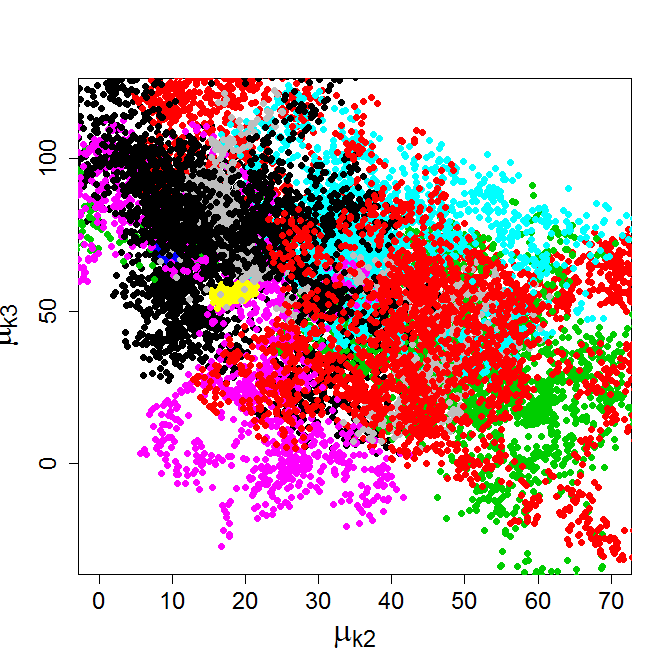
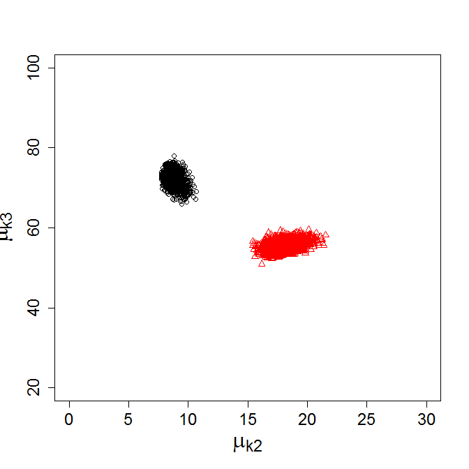
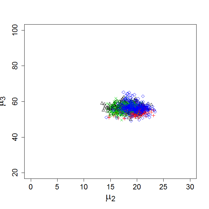
Figure B.4: AIS data set, $K=10$, $L=4$, $\phi_{B}=0.5$, $\phi_{W}=0.1$: Point process representation of the cluster means $\boldsymbol{\mu}_{k}$ of all 10 clusters (left-hand side) and only from those where $\hat{K}_{0}=2$ (middle). Right-hand side: Point process representation of the means of all subcomponents forming the cluster in the bottom right in the plot in the middle.

Appendix C Simulation studies

For both simulation studies, 10 data sets are generated and a sparse hierarchical mixture of mixtures model is estimated. Prior distributions and hyperparameters are specified as described in Section 2.1 and 2.3. MCMC sampling is run for $M=4000$ iterations after a burn-in of $4000$ draws. For the sampling, the starting classification of the observations is obtained by first clustering the observations into $K$ groups using $K$-means clustering and by then allocating the observations within each group to the $L$ subcomponents by using $K$-means clustering again. The estimated number of clusters is reported in Tables C.2 and C.3, where in parentheses the number of data sets for which this number is estimated is given.

C.1 Simulation setup I

The simulation setup I consists of drawing samples with 800 observations grouped in four clusters. Each cluster is generated by a normal mixture with a different number of subcomponents. The four clusters are generated by sampling from an eight-component normal mixture with component means

$$(\boldsymbol{\mu}_{1}\quad\boldsymbol{\mu}_{2}\quad\ldots\quad\boldsymbol{\mu}_{8})=\begin{pmatrix}6&4&8&22.5&20&22&22&6.5\\ 1.5&6&6&1.5&8&31&31&29\end{pmatrix},$$

variance-covariance matrices

$$\boldsymbol{\Sigma}_{1} =\begin{pmatrix}4.84&0\\ 0&2.89\end{pmatrix}, \boldsymbol{\Sigma}_{2} =\begin{pmatrix}3.61&5.05\\ 5.05&14.44\end{pmatrix}, \boldsymbol{\Sigma}_{3} =\begin{pmatrix}3.61&-5.05\\ -5.05&14.44\end{pmatrix},$$

$$\boldsymbol{\Sigma}_{4} =\begin{pmatrix}12.25&0\\ 0&3.24\end{pmatrix}, \boldsymbol{\Sigma}_{5} =\begin{pmatrix}3.24&0\\ 0&12.25\end{pmatrix}, \boldsymbol{\Sigma}_{6} =\begin{pmatrix}14.44&0\\ 0&2.25\end{pmatrix},$$

$$\boldsymbol{\Sigma}_{7} =\begin{pmatrix}2.25&0\\ 0&17.64\end{pmatrix}, \boldsymbol{\Sigma}_{8} =\begin{pmatrix}2.25&4.2\\ 4.20&16.0\end{pmatrix},$$

and weight vector $\boldsymbol{\eta}=1/4(1/3,1/3,1/3,1/2,1/2,1/2,1/2,1)$.

In Figure C.5 the scatter plot of one data set and the 90% probability contour lines of the generating subcomponent distributions are shown. The first three normal distributions generate the triangle-shaped cluster, the next two the L-shaped cluster, and the last three distributions the cross-shaped and the elliptical cluster. The number of generating distributions for each cluster (clockwise from top left) is 1, 2, 2, and 3. This simulation setup is inspired by Baudry et al. (2010) who use clusters similar to the elliptical and cross-shaped clusters on the top of the scatter plot in Figure C.5. However, our simulation setup is expanded by the two clusters at the bottom which have a triangle and an $L$ shape. Our aim is to recover the four clusters.

If we estimate a sparse finite mixture model (see Malsiner-Walli et al., 2016), which can be seen as a special case of the sparse hierarchical mixture of mixtures model with number of subcomponents $L=1$, the estimated number of components is seven, as can be seen in the classification results shown in Figure C.5 in the middle plot. This is to be expected, as by specifying a standard normal mixture the number of generating normal distributions is estimated rather than the number of data clusters. In contrast, if a sparse hierarchical mixture of mixtures model with $K=10$ clusters and $L=4$ subcomponents is fitted to the data, all but four clusters become empty during MCMC sampling and the four data clusters are captured rather well, as can be seen in the classification plot in Figure C.5 on the right-hand side.

In order to study the effect of changing the specified maximum number of clusters $K$ and subcomponents $L$ on the estimation result, a simulation study consisting of 10 data sets with the simulation setup as explained above and varying numbers of clusters $K=4,10,15$ and subcomponents $L=1,3,4,5$ is performed. For each combination of $K$ and $L$ the estimated number of clusters is reported in Table C.2.

First we study the effect of the number of specified subcomponents $L$ on the estimated number of data clusters. As can be seen in Table C.2, we are able to identify the true number of clusters if the number of subcomponents $L$ forming a cluster is at least three. I.e. by specifying an overfitting mixture with $K=10$ clusters, for (almost) all data sets superfluous clusters become empty and using the most frequent number of non-empty clusters as an estimate for the true number of data clusters gives good results. If a sparse finite normal mixture is fitted to the data, for almost all data sets 7 normal components are estimated. Regarding the maximum number of clusters $K$ in the overfitting mixture, the estimation results do scarcely change if this number is increased to $K=15$, as can be seen in the last row of Table C.2. This means that also in a highly overfitting mixture, all superfluous clusters become empty during MCMC sampling.

In Figure C.6, the effect of the number of subcomponents $L$ on the resulting cluster distributions is studied. For the data set shown in Figure C.5, for an increasing number of subcomponents the estimated cluster distributions are plotted using the MAP estimates of the weights, means and covariance matrices of the subcomponents. The estimated cluster distributions look quite similar, regardless of the size of $L$. This robustness may be due to the smoothing effect of the specified hyperpriors.

	1		3		4		5
4	4(10)		4(10)		4(10)		4(10)
10	7(9)		4(10)		4(10)		4(10)
	6(1)
15	7(9)		4(10)		4(9)		4(10)
	8(1)				5(1)

Table C.2: Simulation setup I (based on 10 data sets); true number of clusters equal to 4. Results for the estimated number of non-empty clusters $\hat{K}_{0}$ for various values of $K$ and $L$. The number of data sets estimating the reported $\hat{K}_{0}$ is given in parentheses.

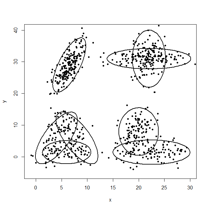
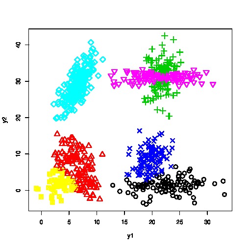
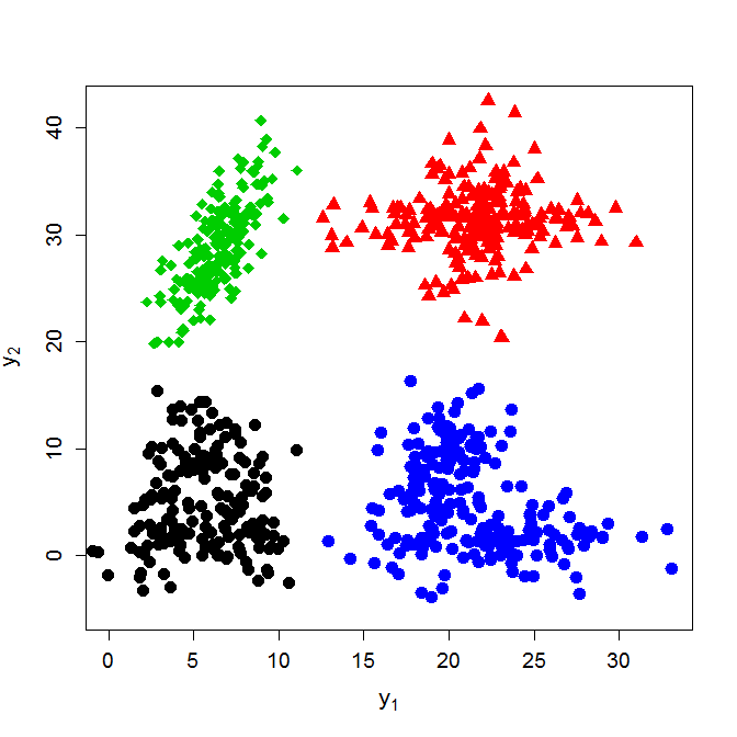
Figure C.5: Simulation setup I. Scatter plot of one data set with the generating component densities shown with 90% probability contour lines (left-hand side), and clustering results by estimating a sparse hierarchical mixture of mixtures model with $K=10$, $L=1$ (middle) and $K=10$, $L=4$ (right-hand side).

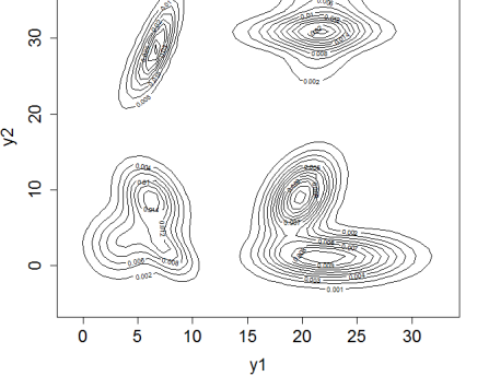
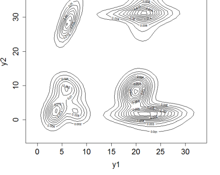
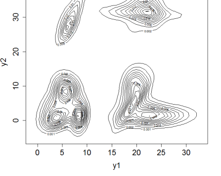
Figure C.6: Simulation setup I, $K=10$, various values of $L$. For the data set in Figure C.5, the estimated cluster distributions (MAP estimates of means, weights, and covariance matrices of the subcomponents) are plotted for an increasing number of specified subcomponents $L=3,4,5$ (from left to right).

C.2 Simulation setup II

In Section 2.3 it is suggested to specify the between-cluster variability by $\phi_{B}=0.5$ and the between-subcomponent variability by $\phi_{W}=0.1$. As can be seen in the previous simulation study in Section C.1 this a priori specification gives promising results if the data clusters are well-separated. However, in contrast to the simulation setup I, in certain applications data clusters might be close or even overlapping. In this case, the clustering result might be sensitive in regard to the specification of $\phi_{B}$ and $\phi_{W}$. Therefore, in the following simulation study it is investigated how the specification of $\phi_{B}$ and $\phi_{W}$ affects the identification of data clusters if they are not well-separated. We want to study how robust the clustering results are against misspecification of the two proportions.

In order to mimic close data clusters, 10 data sets with 300 observations are generated from a three-component normal mixture, where, however, only two data clusters can be clearly distinguished. In Figure C.7 the scatter plot of one data set is displayed. The 300 observations are sampled from a normal mixture with component means

$$(\boldsymbol{\mu}_{1}\quad\boldsymbol{\mu}_{2}\quad\boldsymbol{\mu}_{3})=\begin{pmatrix}2&4.2&7.8\\ 2&4.2&7.8\end{pmatrix},$$

variance-covariance matrices $\boldsymbol{\Sigma}_{1}=\boldsymbol{\Sigma}_{2}=\boldsymbol{\Sigma}_{3}=\mathbf{I}_{2}$ and equal weights $\boldsymbol{\eta}=(1/3,1/3,1/3)$.

For various values of $\phi_{B}$ (between 0.1 and 0.9) and $\phi_{W}$ (between 0.01 and 0.4) a sparse mixture of mixtures model with $K=10$ clusters and $L=4$ subcomponents is fitted and the number of clusters is estimated. For each combination of $\phi_{B}$ and $\phi_{W}$ the results are reported in Table C.3.

Table C.3 indicates that if $\phi_{B}$ increases, also $\phi_{W}$ has to increase in order to identify exactly two clusters. This makes sense since by increasing $\phi_{B}$ the a priori within-cluster variability becomes smaller yielding tight subcomponent densities. Tight subcomponents in turn require a large proportion $\phi_{W}$ of variability explained by the subcomponent means to capture the whole cluster. Thus $\phi_{W}$ has to be increased too. However, $\phi_{W}$ has to be selected carefully. If $\phi_{W}$ is larger than actually needed, some subcomponents are likely to “emigrate” to neighboring clusters. This leads finally to only one cluster being estimated for some data sets. This is basically the case for some of the combinations of $\phi_{B}$ and $\phi_{W}$ displayed in the upper triangle of the table. In contrast, if $\phi_{W}$ is smaller than needed, due to the induced shrinkage of the subcomponent means toward the cluster center, the specified cluster mixture distribution is not able to fit the whole data cluster and two cluster distributions are needed to fit a single data cluster. This can be seen for some of the combinations of $\phi_{B}$ and $\phi_{W}$ displayed in the lower triangle of the table.

	0.01	0.1	0.2	0.3	0.4
0.1	3(6)	2(10)	2(5)	1(8)	1(8)
	2(4)		1(5)	2(2)	2(2)
0.3	3(6)	2(10)	2(8)	2(6)	1(7)
	2(4)		1(2)	1(4)	2(3)
0.5	3(5)	2(10)	2(10)	2(9)	2(7)
	2(5)			1(1)	1(3)
0.7	3(7)	2(7)	2(10)	2(10)	2(10)
	2(3)	3(3)
0.9	3(6)	3(7)	3(5)	2(8)	2(10)
	4(4)	2(3)	2(5)	3(2)

Table C.3: Simulation setup II (based on 10 data sets); true number of clusters equal to 2, $K=10$, $L=4$. Results for the estimated number of non-empty clusters $\hat{K}_{0}$ for various amounts of $\phi_{B}$ and $\phi_{W}$. The number of data sets estimating the reported $\hat{K}_{0}$ is given in parentheses.

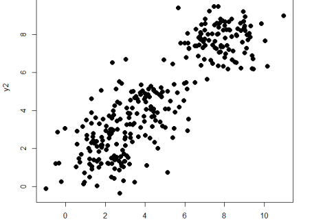
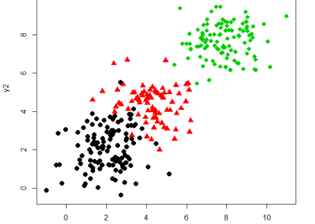
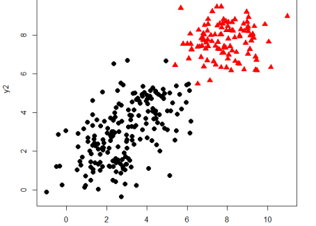
Figure C.7: Simulation setup II. Scatter plot of one data set (left-hand side), classification according to the generating distributions (middle) and to the clusters obtained from a mixture of mixtures with $K=10$, $L=4$, $\phi_{B}=0.5$ and $\phi_{W}=0.1$ (right-hand side).

Appendix D Description of the data sets

The following data sets are investigated. The Yeast data set (Nakai and Kanehisa, 1991) aims at predicting the cellular localization sites of proteins and can be downloaded from the UCI machine learning repository (Bache and Lichman, 2013). As in Franczak et al. (2012), we aim at distinguishing between the two localization sites CYT (cytosolic or cytoskeletal) and ME3 (membrane protein, no N-terminal signal) by considering a subset of three variables, namely McGeoch’s method for signal sequence (mcg), the score of the ALOM membrane spanning region prediction program (alm) and the score of discriminant analysis of the amino acid content of vacuolar and extracellular proteins (vac).

The Flea beetles data set (Lubischew, 1962) considers 6 physical measurements of 74 male flea beetles belonging to three different species. It is available in the R package DPpackage (Jara et al., 2011).

The Australian Institute of Sport (AIS) data set (Cook and Weisberg, 1994) consists of 11 physical measurements on 202 athletes (100 female and 102 male). As in Lee and McLachlan (2013a), we only consider three variables, namely body mass index (BMI), lean body mass (LBM) and the percentage of body fat (Bfat). The data set is contained in the R package locfit (Loader, 2013).

The Breast Cancer Wisconsin (Diagnostic) data set (Mangasarian et al., 1995) describes characteristics of the cell nuclei present in images. The clustering aim is to distinguish between benign and malignant tumors. It can be downloaded from the UCI machine learning repository. Following Fraley and Raftery (2002) and Viroli (2010) we use a subset of three attributes: extreme area, extreme smoothness, and mean texture. Additionally, we scaled the data.

The artificial flower data set reported by Yerebakan et al. (2014) can be downloaded from https://github.com/halidziya/I2GMM. It consists of $17000$ two-dimensional observations representing a flower shape. The data set is generated by seventeen Gaussian densities forming 4 clusters: nine components generate the blossom of the flower, four components the stem and two components each of the two leaves. Note that within each cluster, the generating components have the same orientation. This specification meets the assumption made in the infinite mixture of infinite mixtures model by Yerebakan et al. (2014). We used a subsample of 400 data points for our application, thus leading to the benchmark data sets all being of comparable size. The scatter plot of the sample is given in Figure D.8 on the left-hand side. If we fit a sparse mixture of mixtures model with $K=10$ clusters and $L=4$ subcomponents and the usual prior settings as described in Section 2, the four clusters of the flower (petal, stem, and two leaves) can be clearly captured, as can be seen in Figure D.8, where the estimated clustering result and the corresponding cluster distributions are shown.

The flow cytometry data set DLBCL contains intensities of markers stained on a sample of over 8000 cells derived from the lymph nodes of patients diagnosed with Diffuse Large B-cell Lymphoma (DLBCL). The aim of the clustering is to group the individual cell data measurements into only a few groups on the basis of similarities in light scattering and fluorescence, see Aghaeepour et al. (2013) for more details. For this data set, class labels of the observations partitioning the data into four classes are available which were obtained by manual partitioning (“gating”). The data set is available in the R package EMMIXuskew (Lee and McLachlan, 2013b) as data set DLBCL with the corresponding class labels in true.clusters.

The flow cytometry data set GvHDB01case by Brinkman et al. (2007) consists of 12442 six-dimensional observations which represent a blood sample from a subject who developed Graft versus Host disease (GvHD). GvHD is a severe complication following a blood and marrow transplantation, when donor immune cells in the graft attack the body cells of the recipient. The data were analyzed first by Brinkman et al. (2007). Lo et al. (2008) fitted a Student-$t$ mixture model to this data and estimated 12 clusters using the EM algorithm. In the Bayesian framework, Frühwirth-Schnatter and Pyne (2010) fitted finite mixtures of skew-normal and skew-$t$ distributions and found 12 and 9 clusters. By comparing this sample to a control sample from a patient who had a similar transplantation but did not develop the disease, Brinkman et al. (2007) found a very small cluster of live cells (high “FSC”, high “SSC”) in the sample with a high expression in the four markers (“CD4+”, “CD8$\beta$+”’, “CD3+”, “CD8+”). This cluster was not present in the control sample and seems to be correlated with the development of GvHD.

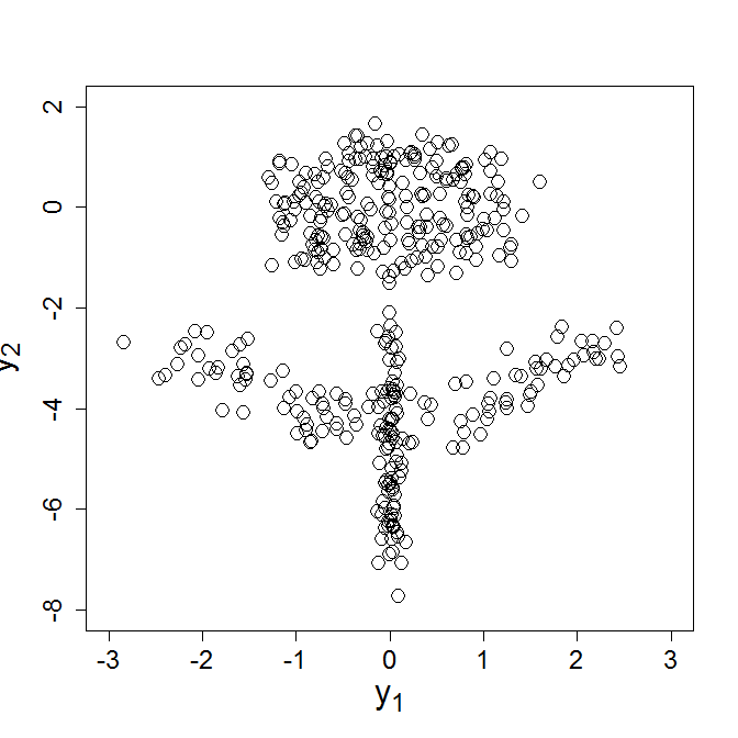
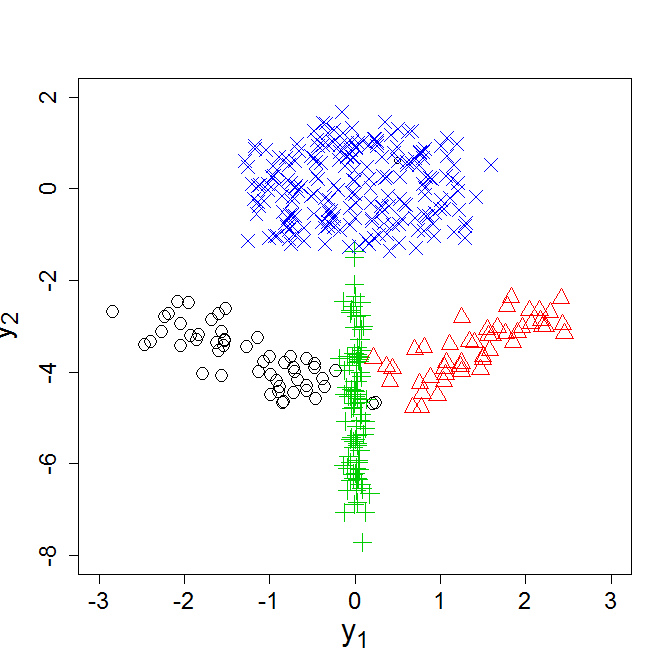
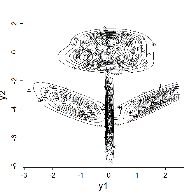
Figure D.8: Flower data set. Boxplot of a sample with 400 data points (left-hand side), the estimated clusters for $K=10,L=4$, $\phi_{B}=0.5,\phi_{W}=0.1,\nu_{1}=\nu_{2}=10$ (middle), and the corresponding cluster distributions (right-hand side).

For the data sets with known class labels, the clustering result of the estimated models is measured by the misclassification rate and the adjusted Rand index (Hubert and Arabie, 1985). To calculate the misclassification rate of the estimated model, the “optimal” matching between the estimated cluster labels and the true known class labels is determined as the one minimizing the misclassification rate over all possible matches for each of the scenarios. The misclassification rate is measured by the number of misclassified observations divided by all observations and should be as small as possible.

The adjusted Rand index (Hubert and Arabie, 1985) is used to assess the similarity between the true and the estimated partition of the data. It is a corrected form of the Rand index (Rand, 1971) which is adjusted for chance agreement. An adjusted Rand index of 1 corresponds to perfect agreement of two partitions whereas an adjusted Rand index of 0 corresponds to results no better than would be expected by randomly drawing two partitions, each with a fixed number of clusters and a fixed number of elements in each cluster.

Appendix E Issues with the merging approach

The merging approach, which consists of first fitting a finite mixture of Gaussians to suitably approximate the data distribution and subsequently combines components to clusters, is susceptible to yield poor classifications, since the resulting clusters can only emerge as the union of components that have been identified in the previous step. For illustration, the AIS data (see Appendix D) are clustered using function clustCombi (Baudry et al., 2010) from the R package mclust (Fraley et al., 2012). The results are shown in Figure E.9. The first step results in a standard Gaussian mixture with three components (left-hand plot), and subsequently all data in the smallest component are merged with one of the bigger components to form two clusters (middle plot) which are not satisfactorily separated from each other due to the misspecification of the standard Gaussian mixture in the first step. In contrast, the sparse hierarchical mixture of mixtures approach we develop in the present paper identifies two well-separated clusters on the upper level of the hierarchy (right-hand plot).

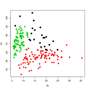
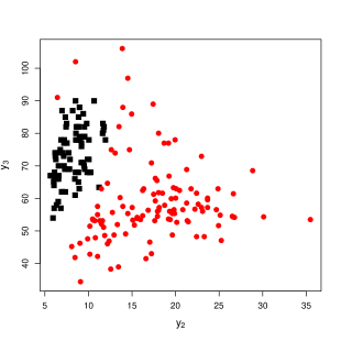
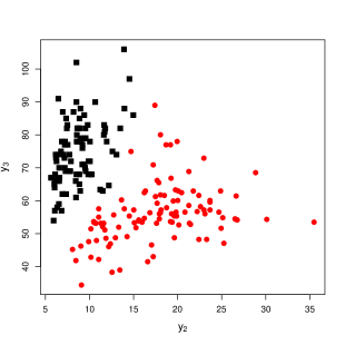
Figure E.9: AIS data set, variables “X.Bfat” and “LBM”. Scatter plots of the observations with different estimated classifications based on Mclust (left-hand side), combiClust (middle), and the sparse hierarchical mixture of mixtures approach developed in this paper ($K=10,L=4$) (right-hand side).

Appendix F Fitting a mixture of two $\mathit{SAL}$ distributions

Although it is not the purpose of our approach to capture non-dense data clusters, we apply it to the challenging cluster shapes generated by shifted asymmetric Laplace ($\mathit{SAL}$) distributions, which are introduced by Franczak et al. (2012) in order to capture asymmetric data clusters with outliers. We sampled data from a mixture of two $\mathit{SAL}$ distributions according to Section 4.2 in Franczak et al. (2012). The data set is shown in Figure F.10 on the left-hand side.

If we fit a sparse hierarchical mixture of mixtures model with $K=10$ clusters and $L=4$ subcomponents and priors and hyperpriors specified as in Sections 2.1 and 2.3, four clusters are estimated, as can be seen in the middle plot of Figure F.10. Evidently, the standard prior setting, tuned to capture dense homogeneous data clusters, performs badly for this kind of clusters. Thus, in order to take the specific data cluster shapes into account, we adjust the prior specifications accordingly. A data cluster generated by a $\mathit{SAL}$ distribution is not homogeneously dense, it rather consists of a relatively dense kernel on one side of the cluster and a non-dense, light and comet-like tail with possibly extreme observations on the other side. Therefore within a cluster, subcomponents with very different covariance matrices are required in order to fit the whole cluster distribution. Since specification of hyperpriors on $\lambda_{kj}$ and $\mathbf{C}_{0k}$ has a smoothing and balancing effect on the subcomponent densities, we omit these hyperprior specifications, and choose fixed values for $k=1,\ldots,K$, i.e. $\mathbf{C}_{0k}=g_{0}\cdot\mathbf{G}_{0}^{-1}$ and $\lambda_{kj}\equiv 1$, $j=1,\ldots,r$.

Additionally, in order to reach also extreme points, we increase both the number of subcomponents to $L=5$ and the a priori variability explained by the subcomponent means to $\phi_{W}=0.2$. At the same time we adjust the proportion of heterogeneity explained by the cluster means by decreasing $\phi_{B}$ to $0.4$, thus keeping the subcomponent covariance matrices large. If we estimate again a sparse hierarchical mixture of mixtures model with these modified prior settings, the two clusters can be identified, see Figure F.10 on the right-hand side.

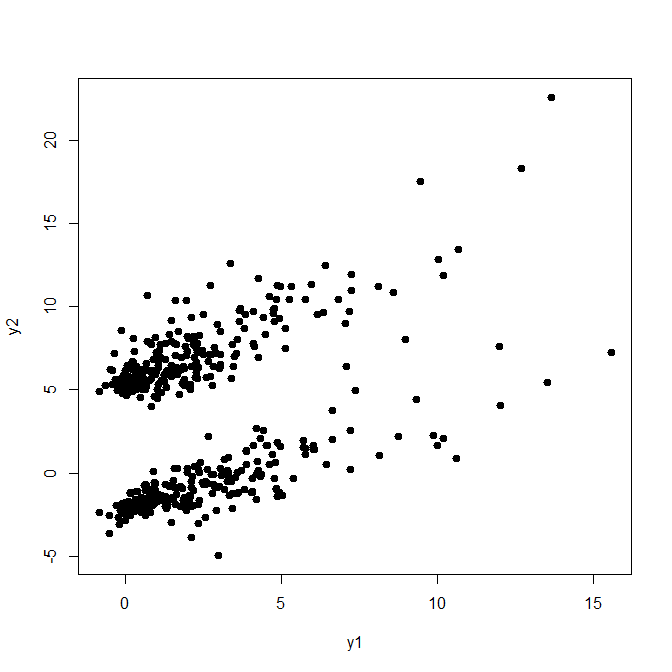
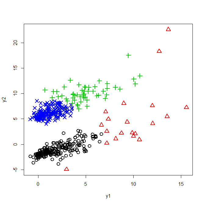
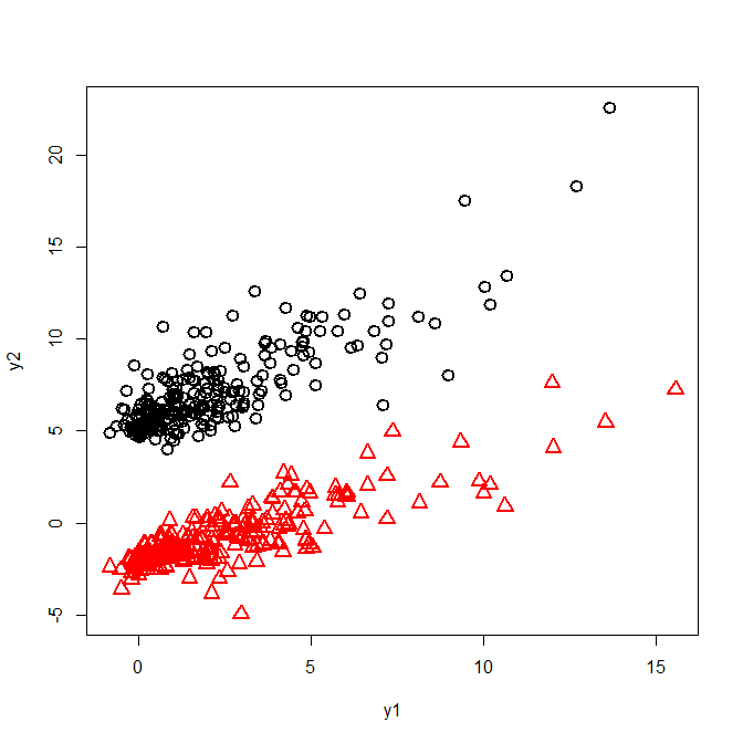
Figure F.10: Samples from a mixture of two $\mathit{SAL}$ distributions (left-hand side), the estimated clusters for $K=10,L=4$, $\phi_{B}=0.5,\phi_{W}=0.1,\nu_{1}=\nu_{2}=10$ (middle), and for $K=10,L=5$, $\phi_{B}=0.4,\phi_{W}=0.2$, with fixed hyperparameters $\mathbf{C}_{0k}=g_{0}\cdot\mathbf{G}_{0}^{-1}$ and $\lambda_{kj}\equiv 1$ (right-hand side).

References

- Aghaeepour et al. (2013) Aghaeepour, N., G. Finak, H. Hoos, T. R. Mosmann, R. Brinkman, R. Gottardo, R. H. Scheuermann, F. Consortium, D. Consortium, et al. (2013). Critical assessment of automated flow cytometry data analysis techniques. Nature methods 10(3), 228–238.
- Argiento et al. (2014) Argiento, R., A. Cremaschi, and A. Guglielmi (2014). A ”density-based” algorithm for cluster analysis using species sampling Gaussian mixture models. Journal of Computational and Graphical Statistics 23(4), 1126–1142.
- Bache and Lichman (2013) Bache, K. and M. Lichman (2013). UCI machine learning repository. URL http://archive.ics.uci.edu/ml.
- Bartolucci (2005) Bartolucci, F. (2005). Clustering univariate observations via mixtures of unimodal normal mixtures. Journal of Classification 22(2), 203–219.
- Baudry et al. (2010) Baudry, J.-P., A. Raftery, G. Celeux, K. Lo, and R. Gottardo (2010). Combining mixture components for clustering. Journal of Computational and Graphical Statistics 2(19), 332–353.
- Brinkman et al. (2007) Brinkman, R. R., M. Gasparetto, S.-J. J. Lee, A. J. Ribickas, J. Perkins, W. Janssen, R. Smiley, and C. Smith (2007). High-content flow cytometry and temporal data analysis for defining a cellular signature of graft-versus-host disease. Biology of Blood and Marrow Transplantation 13(6), 691–700.
- Celeux and Soromenho (1996) Celeux, G. and G. Soromenho (1996). An entropy criterion for assessing the number of clusters in a mixture model. Journal of classification 13(2), 195–212.
- Chan et al. (2008) Chan, C., F. Feng, J. Ottinger, D. Foster, M. West, and T. B. Kepler (2008). Statistical mixture modelling for cell subtype identification in flow cytometry. Cytometry, A 73, 693–701.
- Cook and Weisberg (1994) Cook, R. D. and S. Weisberg (1994). An Introduction to Regression Graphics. Wiley.
- Dahl (2006) Dahl, D. B. (2006). Model-based clustering for expression data via a Dirichlet process mixture model. In Bayesian Inference for Gene Expression and Proteomics, pp. 201–218. Cambridge University Press.
- Di Zio et al. (2007) Di Zio, M., U. Guarnera, and R. Rocci (2007). A mixture of mixture models for a classification problem: The unity measure error. Computational Statistics & Data Analysis 51(5), 2573–2585.
- Escobar and West (1995) Escobar, M. D. and M. West (1995). Bayesian density estimation and inference using mixtures. Journal of the American Statistical Association 90(430), 577–588.
- Fall and Barat (2014) Fall, M. D. and E. Barat (2014). Gibbs sampling methods for Pitman-Yor mixture models. <hal-00740770v2>.
- Ferguson (1983) Ferguson, T. S. (1983). Bayesian density estimation by mixtures of normal distributions. In M. H. Rizvi and J. S. Rustagi (Eds.), Recent Advances in Statistics: Papers in Honor of Herman Chernov on His Sixtieth Birthday, pp. 287–302. New York: Academic Press.
- Fraley and Raftery (2002) Fraley, C. and A. E. Raftery (2002). Model-based clustering, discriminant analysis, and density estimation. Journal of the American Statistical Association 97(458), 611–631.
- Fraley et al. (2012) Fraley, C., A. E. Raftery, T. B. Murphy, and L. Scrucca (2012). mclust Version 4 for R: Normal Mixture Modeling for Model-Based Clustering, Classification, and Density Estimation. Technical Report 597, Department of Statistics, University of Washington.
- Franczak et al. (2012) Franczak, B. C., R. P. Browne, and P. D. McNicholas (2012). Mixtures of shifted asymmetric Laplace distributions. eprint arXiv:1207.1727.
- Frühwirth-Schnatter (2004) Frühwirth-Schnatter, S. (2004). Estimating marginal likelihoods for mixture and Markov switching models using bridge sampling techniques. The Econometrics Journal 7, 143–167.
- Frühwirth-Schnatter (2006) Frühwirth-Schnatter, S. (2006). Finite Mixture and Markov Switching Models. New York: Springer.
- Frühwirth-Schnatter (2011) Frühwirth-Schnatter, S. (2011). Label switching under model uncertainty. In K. Mengerson, C. Robert, and D. Titterington (Eds.), Mixtures: Estimation and Application, pp. 213–239. Wiley.
- Frühwirth-Schnatter (2011) Frühwirth-Schnatter, S. (2011). Panel data analysis – a survey on model-based clustering of time series. Advances in Data Analysis and Classification 5, 251–280.
- Frühwirth-Schnatter and Pyne (2010) Frühwirth-Schnatter, S. and S. Pyne (2010). Bayesian inference for finite mixtures of univariate and multivariate skew-normal and skew-t distributions. Biostatistics 11(2), 317–336.
- Green and Richardson (2001) Green, P. J. and S. Richardson (2001). Modelling heterogeneity with and without the Dirichlet process. Scandinavian Journal of Statistics 28, 355–375.
- Griffin and Brown (2010) Griffin, J. E. and P. J. Brown (2010). Inference with normal-gamma prior distributions in regression problems. Bayesian Analysis 5(1), 171–188.
- Hartigan and Wong (1979) Hartigan, J. A. and M. A. Wong (1979). Algorithm AS136: A -means clustering algorithm. Applied Statistics 28(1), 100–108.
- Hennig (2010) Hennig, C. (2010). Methods for merging Gaussian mixture components. Advances in Data Analysis and Classification 4(1), 3–34.
- Hubert and Arabie (1985) Hubert, L. and P. Arabie (1985). Comparing partitions. Journal of Classification 2(1), 193–218.
- Jara et al. (2011) Jara, A., T. E. Hanson, F. A. Quintana, P. Müller, and G. L. Rosner (2011). DPpackage: Bayesian semi- and nonparametric modeling in R. Journal of Statistical Software 40(5), 1.
- Jasra et al. (2005) Jasra, A., C. C. Holmes, and D. A. Stephens (2005). Markov chain Monte Carlo methods and the label switching problem in Bayesian mixture modelling. Statistical Science 20(1), 50–67.
- Korwar and Hollander (1973) Korwar, R. M. and M. Hollander (1973). Contributions to the theory of Dirichlet processes. The Annals of Probability 1(4), 705–711.
- Lau and Green (2007) Lau, J. W. and P. Green (2007). Bayesian model-based clustering procedures. Journal of Computational and Graphical Statistics 16, 526–558.
- Lee and McLachlan (2013a) Lee, S. and G. J. McLachlan (2013a). Model-based clustering and classification with non-normal mixture distributions. Statistical Methods and Applications 22(4), 427–454.
- Lee and McLachlan (2014) Lee, S. and G. J. McLachlan (2014). Finite mixtures of multivariate skew -distributions: Some recent and new results. Statistics and Computing 24(2), 181–202.
- Lee and McLachlan (2013b) Lee, S. X. and G. J. McLachlan (2013b). EMMIX-uskew: an R package for fitting mixtures of multivariate skew t-distributions via the EM algorithm. Journal of Statistical Software 55(12).
- Leisch (2006) Leisch, F. (2006). A toolbox for -centroids cluster analysis. Computational Statistics & Data Analysis 51(2), 526–544.
- Li (2005) Li, J. (2005). Clustering based on a multilayer mixture model. Journal of Computational and Graphical Statistics 3(14), 547–568.
- Liverani et al. (2015) Liverani, S., D. I. Hastie, L. Azizi, M. Papathomas, and S. Richardson (2015). PReMiuM: An R package for profile regression mixture models using Dirichlet processes. Journal of Statistical Software 64(7), 1–30.
- Lo et al. (2008) Lo, K., R. R. Brinkman, and R. Gottardo (2008). Automated gating of flow cytometry data via robust model-based clustering. Cytometry Part A 73(4), 321–332.
- Loader (2013) Loader, C. (2013). locfit: Local Regression, Likelihood and Density Estimation. R package version 1.5-9.1.
- Lubischew (1962) Lubischew, A. A. (1962). On the use of discriminant functions in taxonomy. Biometrics 18(4), 455–477.
- Malsiner-Walli et al. (2016) Malsiner-Walli, G., S. Frühwirth-Schnatter, and B. Grün (2016). Model-based clustering based on sparse finite Gaussian mixtures. Statistics and Computing 26, 303–324.
- Mangasarian et al. (1995) Mangasarian, O. L., W. N. Street, and W. H. Wolberg (1995). Breast cancer diagnosis and prognosis via linear programming. Operations Research 43(4), 570–577.
- Medvedovic et al. (2004) Medvedovic, M., K. Y. Yeung, and R. E. Bumgarner (2004). Bayesian mixture model based clustering of replicated microarray data. Bioinformatics 20(8), 1222–1232.
- Melnykov (2016) Melnykov, V. (2016). Merging mixture components for clustering through pairwise overlap. Journal of Computational and Graphical Statistics 25, 66–90.
- Molitor et al. (2010) Molitor, J., M. Papathomas, M. Jerrett, and S. Richardson (2010). Bayesian profile regression with an application to the National survey of children’s health. Biostatistics 11, 484–498.
- Müller and Mitra (2013) Müller, P. and R. Mitra (2013). Bayesian nonparametric inference –- Why and how. Bayesian Analysis 8(2), 269–302.
- Nakai and Kanehisa (1991) Nakai, K. and M. Kanehisa (1991). Expert system for predicting protein localization sites in gram-negative bacteria. Proteins: Structure, Function, and Bioinformatics 11(2), 95–110.
- Nobile (2004) Nobile, A. (2004). On the posterior distribution of the number of components in a finite mixture. The Annals of Statistics 32(5), 2044–2073.
- Papastamoulis (2015) Papastamoulis, P. (2015). label.switching: Relabelling MCMC Outputs of Mixture Models. R package version 1.4.
- Pitman and Yor (1997) Pitman, J. and M. Yor (1997). The two-parameter Poisson-Dirichlet distribution derived from a stable subordinator. Annals of Probability 25, 855–900.
- Quintana and Iglesias (2003) Quintana, F. A. and P. L. Iglesias (2003). Bayesian clustering and product partion models. Journal of the Royal Statistical Society B 65, 557–574.
- Rand (1971) Rand, W. M. (1971). Objective criteria for the evaluation of clustering methods. Journal of the American Statistical Association 66(336), 846–850.
- Rodriguez et al. (2008) Rodriguez, A., D. B. Dunson, and A. E. Gelfand (2008). The nested Dirichlet process. Journal of the American Statistical Association 103(483), 1131–1154.
- Rousseau and Mengersen (2011) Rousseau, J. and K. Mengersen (2011). Asymptotic behaviour of the posterior distribution in overfitted mixture models. Journal of the Royal Statistical Society B 73(5), 689–710.
- Sethuraman (1994) Sethuraman, J. (1994). A constructive definition of Dirichlet priors. Statistica Sinica 4, 639–650.
- Teh et al. (2006) Teh, Y. W., M. I. Jordan, M. J. Beal, and D. M. Blei (2006). Hierarchical Dirichlet processes. Journal of the American Statistical Association 101(476), 1566–1581.
- Viroli (2010) Viroli, C. (2010). Dimensionally reduced model-based clustering through mixtures of factor mixtures analyzers. Journal of Classification 27(3), 363–388.
- Vrbik and McNicholas (2014) Vrbik, I. and P. D. McNicholas (2014). Parsimonious skew mixture models for model-based clustering and classification. Computational Statistics & Data Analysis 71, 196–210.
- Yerebakan et al. (2014) Yerebakan, H. Z., B. Rajwa, and M. Dundar (2014). The infinite mixture of infinite Gaussian mixtures. In Advances in Neural Information Processing Systems, pp. 28–36.