Cosmological Analysis of Pilgrim Dark Energy in Loop Quantum Cosmology

Abstract

The proposal of pilgrim dark energy is based on speculation that phantom-like dark energy (with strong enough resistive force) can prevent black hole formation in the universe. We explore this phenomenon in loop quantum cosmology framework by taking Hubble horizon as an infra-red cutoff in pilgrim dark energy. We evaluate the cosmological parameters such as Hubble, equation of state parameter, squared speed of sound and also cosmological planes like $\omega_{\vartheta}-\omega^{\prime}_{\vartheta}$ and $r-s$ on the basis of pilgrim dark energy parameter ($u$) and interacting parameter ($d^{2}$). It is found that values of Hubble parameter lies in the range $74^{+0.005}_{-0.005}$. It is mentioned here that equation state parameter lies within the ranges $-1\mp 0.00005$ for $u=2,~{}1$ and $(-1.12,-1),~{}(-5,-1)$ for $u=-1,-2$, respectively. Also, $\omega_{\vartheta}-\omega^{\prime}_{\vartheta}$ planes provide $\Lambda$CDM limit, freezing and thawing regions for all cases of $u$. It is also interesting to mention here that $\omega_{\vartheta}-\omega^{\prime}_{\vartheta}$ planes lie in the range ($\omega_{\vartheta}=-1.13^{+0.24}_{-0.25},~{}\omega^{\prime}_{\vartheta}<1.32$). In addition, $r-s$ planes also corresponds to $\Lambda$CDM for all cases of $u$. Finally, it is remarked that all the above constraints of cosmological parameters shows consistency with different observational data like Planck, WP, BAO, $H_{0}$ and SNLS.

Keywords: Loop quantum cosmology; Pilgrim dark energy; Cold dark matter; Cosmological parameters.
PACS: 95.36.+d; 98.80.-k.

1 Introduction

The accelerated expansion of the universe is one of the biggest achievements in the subject of cosmology [1]. This expansion phenomenon follows through mysterious form of force called dark energy (DE). However, the nature of DE is still unknown. Different researchers have tried to explore the nature of DE through various aspects via theoretical and observational ways. As a result, they proposed different dynamical DE models as well as modified theories of gravity. The dynamical DE models have been developed in the scenarios of general relativity and quantum gravity. The pioneer candidate of DE is cosmological constant but it has two severe problems [2]. As an alternative to this candidate, the proposals of family of chaplygin gas [3], holographic [4, 5], new agegraphic [6], polytropic gas [7], pilgrim [8]-[10] DE models have been come forward.

The holographic DE (HDE) has become an attractive DE model nowadays, which is developed in the context of quantum gravity and widely used in solving the cosmological problems. The main idea of this model has come from holographic principle which is stated as the number of degrees of freedom of a physical system should scale with its bounding area rather than its volume [11]. With the help of this principle, a relationship between ultraviolet and infrared (IR) cutoffs has been proposed by suggesting that the size of a system should not exceed the mass of black hole (BH) of the same size [12]. By using this relationship, Li [5] developed HDE density as follows

$$\rho_{\Lambda}=3n^{2}M^{2}_{p}L^{-2},$$

here, $n,~{}M_{p},~{}L$ indicate HDE constant, the reduced Planck constant, IR cutoff, respectively. On the basis of compatibility of HDE with the present day observations, different IR cutoffs have been proposed which includes Hubble, particle, event horizons, conformal age of the universe, Ricci scalar, Granda-Oliveros and higher derivative of Hubble parameter [13]-[15] etc.

According to Cohen et al. [12], the bound of energy density from the idea of formation of BH in quantum gravity. However, it is suggested formation of BH can be avoided through appropriate repulsive force which resists the matter collapse phenomenon. This force can only provide phantom DE in spite of other phases of DE like vacuum and quintessence DE. By keeping in mind this phenomenon, Wei [8] has suggested the DE model called pilgrim DE (PDE) on the speculation that phantom DE possesses the large negative pressure as compared to the quintessence DE which helps in violating the null energy condition and possibly prevent the formation of BH. In the past, many applications of phantom DE exist in the literature. For instance, phantom DE is also play an important role in the wormhole physics where the event horizon can be avoided due to its presence [16].

Also, it plays role in the reduction of mass due to its accretion process onto BH. Many works have been done in this support through a family of chaplygin gas [17]. It was also argued in the context of scalar field that BH area reduces up to 50 percent through phantom scalar field accretion onto it [18]. According to Sun [19], mass of BH tends to zero when the universe approaches to big rip singularity. It was also suggested that BHs might not be exist in the universe in the presence of quintessence-like DE which violates only strong energy condition [20]. However, these works do not correspond to reality because quintessence DE does not contain enough resistive force to in order to avoid the formation of BH.

The above discussion is motivated to Wei [8] in developing the PDE model. He analyzed this model with Hubble horizon through different theoretical as well as observational aspects. Also, Saridakis et al. [21]-[30] have discussed the widely the crossing of phantom divide line, quintom as well as phantom-like nature of the universe in different frameworks and found interesting results in this respect. Recently, we have investigated this model by taking different IR cutoffs in flat as well as non-flat FRW universe with different cosmological parameters as well as cosmological planes [9, 10]. This model has also been investigated in different modified gravities [31]-[33]. In the present paper, we check the role of PDE in loop quantum cosmology (LQC). We develop different cosmological parameters and planes. The format of the paper is as follows. In the next section, we provide the basic equations corresponding to PDE models. Also, we discuss the Hubble parameter, EoS parameter and squared speed of sound in section 3. Section 4 explores $\omega_{\vartheta}-\omega_{\vartheta}^{\prime}$ as well as statefinders planes. In the last section, we summarize our results.

2 Loop Quantum Cosmology and Pilgrim Dark Energy

Nowadays, the discussion of DE phenomenon has also been done widely in the context of LQC to describe the quantum effects on our universe. The LQC is an interesting and attractive application of the Loop Quantum Gravity in the cosmological framework and it possesses the properties of non-perturbative and background independent quantization of gravity [34]-[39]. In recent years, many DE models have been studied in the scenario of LQC [40, 41]. Jamil et al. [42] have explored cosmic coincidence problem phenomenon of modern cosmology by taking modified chaplygin gas coupled to dark matter. Also, some authors found that the future singularity appearing in the standard FRW cosmology can be avoided by loop quantum effects [43]. Chakraborty et al. [44] have made observational study of modified chaplygin gas in LQC. Here, we develop basic scenario of interacting PDE (with Hubble horzion) with cold dark matter (CDM) in LQC. The equation of motion in LQC has the form

$$H^{2}=\frac{1}{3m^{2}_{pl}}\rho\left(1-\frac{\rho}{\rho_{c}}\right),$$ (1)

where $\rho$ indicates the sum of CDM and PDE densities. Also, $\rho_{c}=\frac{\sqrt{3}}{16\pi^{2}\gamma^{3}G^{2}\hbar}$ represents the critical loop quantum density, $\gamma$ appears as dimensionless Barbero-Immirzi parameter. It is predicted that the big bang, big rip and other future singularities at semi classical regime can be avoided in LQC. Moreover, the modification in standard FRW cosmology due to LQC becomes more dominant and the universe begins to bounce and then oscillate forever.

It is argued that phantom DE with strong negative pressure can push the universe towards the big rip singularity where all the physical objects lose the gravitational bounds and finally dispersed. The PDE model is also developed in the favor of this scenario which is defined as

$$\rho_{\vartheta}=3n^{2}m_{p}^{4-u}L^{-u},$$ (2)

here $u$ represents the PDE parameter. Wei explored the PDE model with different possible theoretical and observational ways to make the BH free phantom universe with Hubble horizon ($L=H^{-1}$) through PDE parameter.

In this work, we also choose PDE with the Hubble horizon which is the pioneer IR cutoff. Initially, it is plagued with a problem that its EoS parameter provides inconsistent behavior with present status of the universe [13]. This deficiency has been settled down with the passage of time by pointing out that HDE with this IR cutoff can explain the present scenario of the universe in the presence of interaction with DM [45]. Also, the results of different cosmological parameters have been established through different observational schemes by choosing HDE model with Hubble scale [46, 47]. Sheykhi [48] has discussed this model by taking interaction with CDM and pointed out that such model possesses the ability to explain the present scenario of the universe.

In this work, we take interaction between PDE with CDM which takes the following form

$$\dot{\rho}_{m}+3H\rho_{m}=\Theta,\quad\dot{\rho}_{\vartheta}+3H(\rho_{\vartheta}+p_{\vartheta})=-\Theta,$$ (3)

where $\Theta$ possesses dynamical nature and appears as interaction term between CDM and PDE. Different forms of this interaction term has been proposed out of which we use the following form

$$\Theta=3d^{2}H\rho_{m},$$ (4)

where $d^{2}$ is an interacting constant which appears as interaction parameter and exchanges the energy between CDM and DE components. This form of interaction term has been explored for energy transfer through different cosmological constraints. The sign of coupling constant decides the decay of energies either DE decays into CDM (when the interacting parameter is positive) or CDM decays into DE (when the interacting parameter is negative). The present analysis from different aspects imply that the phenomenon of DE decays into CDM which is more acceptable and favors the observational data. Hence, the Eqs. (3) and (4) give

$$\rho_{m}=\rho_{m0}a^{3(d^{2}-1)}.$$ (5)

Also, by taking the differentiation of $\rho_{\vartheta}$ (with Hubble horizon) with respect to $x=\ln a$, we get

$$\rho^{\prime}_{\vartheta}=u\rho_{\vartheta}\frac{\dot{H}}{H^{2}}.$$ (6)

3 Cosmological Parameters in LQC

In this section, we will discuss the physical significance of cosmological parameters corresponding to PDE with Hubble horizon in LQC scenario.

3.1 Hubble Parameter

In order to check the behavior of Hubble parameter in this framework, we can find the following expression after some calculations

$$\frac{\dot{H}}{H^{2}}=-\frac{\rho_{m}}{M^{2}_{p}H^{2}(a)}\left[\frac{2\rho_{c}}{\rho_{c}-2(\rho_{\vartheta}+\rho_{m})}-\frac{u\rho_{\vartheta}}{3M^{2}_{p}H^{2}(a)}\right].$$ (7)

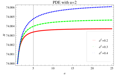
Figure 1: Plot of $H$ versus $a$ for PDE in LQC with $u=2$.

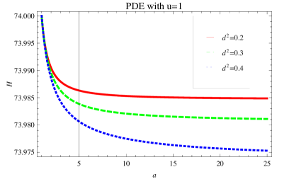
Figure 2: Plot of $H$ versus $a$ for PDE in LQC with $u=1$.

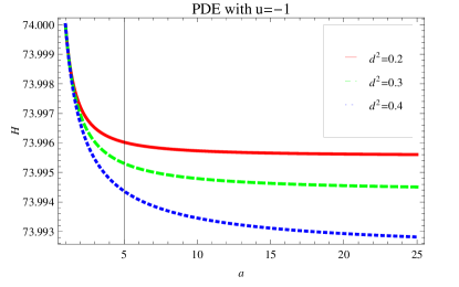
Figure 3: Plot of $H$ versus $a$ for PDE in LQC with $u=-1$.

Figure 4: Plot of $H$ versus $a$ in LQC with $u=-2$.

We solve the above differential equation (7) numerically by using Eqs.(1)-(7) in terms of $H$ and plot it against scale factor $a$ for four different values of $u=2,~{}1,-1,-2$ as shown in Figures 1-4. The initial condition of $H$ is taken as $H[a_{0}]\simeq 74$ as mentioned in Planck observations [49]. It has been greatly improved the precision of the cosmic distance scale through two recent analysis. Riess et al. [50] use HST observations of Cepheid variables in the host galaxies of eight SNe Ia to calibrate the supernova magnitude-redshift relation. Their best estimate of the Hubble constant, from fitting the calibrated SNe magnitude-redshift relation, is

$$H_{0} = 73.8\pm 2.4kms^{-1}Mpc^{-1}~{}~{}~{}~{}~{}~{}~{}\text{(Cepheids+SNe Ia)},$$

where the error is $1\sigma$ level and includes known sources of systematic errors. Freedman et al. [51], as part of the Carnegie Hubble Program, use Spitzer Space Telescope mid-infrared observations to recalibrate secondary distance methods used in the HST Key Project. These authors find

$$H_{0}=[74.3\pm 1.5\text{(statistical)}\pm 2.1\text{(systematic)}]kms^{-1}Mpc^{-1}$$

$$\text{(Carnegie HP)}.$$

In the present paper, it can be observed that the trajectories of Hubble parameter $H(a)$ attains the values approximately to $74^{+0.005}_{-0.005}$. Hence, the present results of Hubble parameter shows consistency with the above results found through observations.

3.2 The Equation of State Parameter

By using all above equations, we can obtain the EoS parameter as

$$\omega_{\vartheta}=-1-d^{2}\frac{\rho_{m}}{\rho_{\vartheta}}+\frac{u\rho_{m}}{3H^{2}(a)}\left[\frac{2\rho_{c}}{\rho_{c}-2(\rho_{\vartheta}+\rho_{m})}-\frac{u\rho_{\vartheta}}{3M^{2}_{p}H^{2}(a)}\right]$$ (8)

The plots of EoS parameter versus $a$ are shown in Figures 5-8 for four different values of $u$. In Figure 5 ($u=2$), the trajectory of $\omega_{\vartheta}$ starts from phantom region and with the passage of time, it approaches to $\Lambda$CDM limit for the interacting cases $d^{2}=0.2,~{}0.3$. However, it remains in the phantom region for the interacting case $d^{2}=0.4$. In case of $u=1$ (Figure 6), the trajectories of EoS parameter remains in quintessence region for $d^{2}=0.4$ while it approaches (from quintessence region) to $\Lambda$CDM limit for the other two cases of $d^{2}$. For $u=-1,-2$ (Figures 7-8), the EoS starts from phantom with comparatively high value and goes towards $\Lambda$CDM limit for $d^{2}=0.2,~{}0.3$ and always remains in phantom for other case of $d^{2}$. Moreover, the constraints on EoS parameter has been put forward by Ade et al. [49] (Planck data)

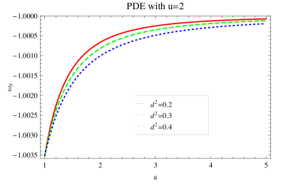
Figure 5: Plot of $\omega_{\vartheta}$ versus $a$ for PDE in LQC with $u=2$.

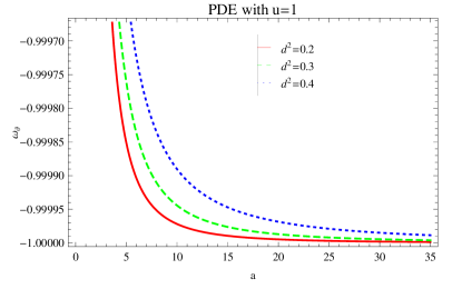
Figure 6: Plot of $\omega_{\vartheta}$ versus $a$ for PDE in LQC with $u=1$.

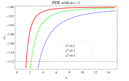
Figure 7: Plot of $\omega_{\vartheta}$ versus $a$ for PDE in LQC with $u=-1$.

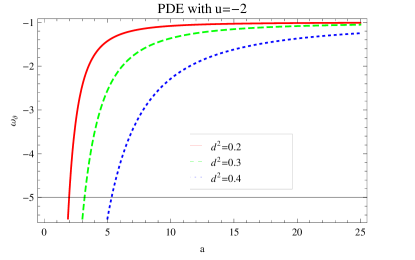
Figure 8: Plot of $\omega_{\vartheta}$ versus $a$ for PDE in LQC with $u=-2$.

$$\omega_{\vartheta} = -1.13^{+0.24}_{-0.25}~{}~{}~{}~{}~{}~{}~{}\text{(Planck+WP+BAO)},$$

$$\omega_{\vartheta} = -1.09\pm 0.17,~{}~{}~{}\text{(Planck+WP+Union 2.1)}$$

$$\omega_{\vartheta} = -1.13^{+0.13}_{-0.14},~{}~{}~{}~{}~{}~{}\text{(Planck+WP+SNLS)},$$

$$\omega_{\vartheta} = -1.24^{+0.18}_{-0.19},~{}~{}~{}~{}~{}~{}\text{(Planck+WP+$H_{0}$)},$$

by implying different combination of observational schemes at $95\%$ confidence level. It can be seen from Figures 5-8 that the EoS parameter also meets the above mentioned values for all cases of interacting parameter which shows consistency of our results. The above discussion shows that all the models provides fully support the PDE phenomenon.

3.3 The Square Speed of Sound

In order to analyze the stability of PDE model in this scenario, we extract the squared speed of sound which is given by

$$\upsilon_{s}^{2}=\frac{\dot{p}}{\dot{\rho}}=\frac{p^{\prime}}{\rho^{\prime}},$$ (9)

where pressure corresponds to PDE only. After some calculations, we can obtain squared speed of sound as follows

$$\upsilon^{2}_{s} = \frac{1}{3}(-3-(a^{-3+3d^{2}}d^{2}\rho_{m0}H(a)^{-u})n^{-2}+(a^{-3+3d^{2}}\rho_{m0}u(-un^{2}$$

$$\times H(a)^{-2+u}+2\rho_{c}(-2a^{-3+3d^{2}}d+\rho_{c}-6n^{2}H(a)^{u})^{-1}))$$

$$\times H^{-2}(a)-(a^{-3+3d^{2}}d^{2}\rho_{m0}u^{2}-(3(-1+d^{2})d^{2}H(a)^{4-u})n^{-2}$$

$$- 3(-1+d^{2})u^{2}n^{2}H(a)^{1+u}-a^{-3+3d^{2}}\rho_{m0}(-3+u)u^{3}n^{4}H(a)^{-3+2u}$$

$$+ (6a^{6}(-1+bs)u\rho_{c}H(a)^{3}(\rho_{c}-6n^{2}H(a)^{u}))(2a^{3d^{2}}\rho_{m0}-a^{3}\alpha$$

$$+ 6a^{3}n^{2}H(a)^{u})^{-2}+(2a^{3d^{2}}d^{2}\rho_{m0}u\rho_{c}H(a)^{2-u})(n^{2}(2a^{3d^{2}}\rho_{m0}-a^{3}\rho_{c}$$

$$+ 6a^{3}n^{2}H(a)^{u}))^{-1}+(2a^{3d^{2}}\rho_{m0}u^{2}\rho_{c}n^{2}H(a)^{-1+u}(-(-4+u)(2a^{3d^{2}}\rho_{m0}$$

$$- a^{3}\rho_{c})+24a^{3}n^{2}H(a)^{u}))(2a^{3d^{2}}\rho_{m0}-a^{3}\rho_{c}+6a^{3}n^{2}H(a)^{u})^{-2}$$

$$+ (4a^{3+3d^{2}}\rho_{m0}u\rho_{c}^{2}H(a)(2a^{3d^{2}}\rho_{m0}-a^{3}\rho_{c}+6a^{3}(1+u)n^{2}H(a)^{u}))(2a^{3d^{2}}$$

$$\times \rho_{m0}-a^{3}\rho_{c}+6a^{3}n^{2}H(a)^{u})^{-3})(auH(a)^{3}(-un^{2}H(a)^{-2+u}$$

$$+ (2\rho_{c})(-2a^{-3+3d^{2}}\rho_{m0}+\rho_{c}-6n^{2}H(a)^{u})^{-1}))^{-1}).$$

The plots of squared speed of sound versus $a$ for three different values of $d^{2}$ and four values of $u=2,~{}1,-1,-2$ is shown in Figures 9-12. It can be observed from Figures 9-10 (for cases $u=2,~{}1$) that the squared speed of sound remains negative for all cases of $d^{2}$ which exhibits the instability of the PDE in LQC scenario. For the cases $u=-1,-2$ (Figures 11-12), it exhibits the stability of the present model for all cases of $d^{2}$.

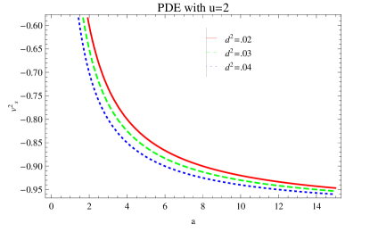
Figure 9: Plot of $\upsilon^{2}_{s}$ versus $a$ for PDE in LQC with $u=2$.

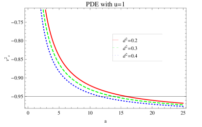
Figure 10: Plot of $\upsilon^{2}_{s}$ versus $a$ for PDE in LQC with $u=1$.

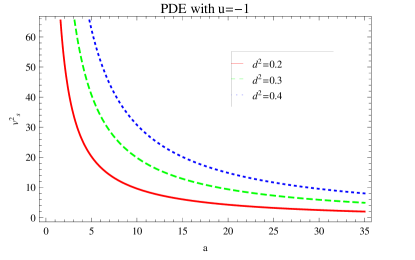
Figure 11: Plot of $\upsilon^{2}_{s}$ versus $a$ for PDE in LQC with $u=-1$.

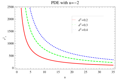
Figure 12: Plot of $\upsilon^{2}_{s}$ versus $a$ for PDE in LQC with $u=-2$.

4 Cosmological Planes in LQC

Here, we will discuss the physical significance of cosmological planes corresponding to PDE with Hubble horizon in LQC scenario.

4.1 $\omega_{\vartheta}-\omega^{\prime}_{\vartheta}$ Analysis

Here, we find the regions on the $\omega_{\vartheta}-\omega^{\prime}_{\vartheta}$ plane ($\omega^{\prime}_{\vartheta}$ represents the evolution of $\omega_{\vartheta}$) as defined by Caldwell and Linder [52] for models under consideration. The models can be categorized in two different classes as thawing and freezing regions on the $\omega_{\vartheta}-\omega^{\prime}_{\vartheta}$ plane. The thawing models describe the region $\omega^{\prime}_{\vartheta}>0$ when $\omega_{\vartheta}<0$ and freezing models represent the region $\omega^{\prime}_{\vartheta}<0$ when $\omega_{\vartheta}<0$. Initially, this phenomenon was applied for analyzing the behavior of quintessence model and found that the corresponding area occupied on the $\omega_{\vartheta}-\omega^{\prime}_{\vartheta}$ plane describes the thawing and freezing regions. Differentiating $\omega_{\vartheta}$ with respect to $x=\ln a$ and after some calculations, we obtain

$$\omega^{\prime}_{\vartheta} = (3H(a)^{4})^{-1}a^{-4+3d^{2}}\rho_{m0}(a^{-3+3d^{2}}d^{4}\rho_{m0}u^{2}-(3(-1+d^{2})d^{4}H(a)^{4-u})$$

$$\times n^{-2}-3(-1+d^{2})u^{2}n^{2}H(a)^{1+u}-a^{-3+3d^{2}}\rho_{m0}(-3+u)u^{3}n^{4}H(a)^{-3+2u}$$

$$+ (6a^{6}(-1+d^{2})u\rho_{c}H(a)^{3}(\rho_{c}-6n^{2}H(a)^{u}))(2a^{3d^{2}}\rho_{m0}-a^{3}\rho_{c}+6a^{3}$$

$$\times n^{2}H(a)^{u})^{-2}+(2a^{3d^{2}}d^{4}\rho_{m0}u\rho_{c}H(a)^{2-u})(n^{2}(2a^{3d^{2}}\rho_{m0}-a^{3}\rho_{c}$$

$$+ 6a^{3}n^{2}H(a)^{u}))^{-2}+(2a^{3d^{2}}\rho_{m0}u^{2}\rho_{c}n^{2}H(a)^{-1+u}(-(-4+u)(2a^{3d^{2}}\rho_{m0}$$

$$- a^{3}\rho_{c})+24a^{3}n^{2}H(a)^{u}))(2a^{3d^{2}}\rho_{m0}-a^{3}\rho_{c}+6a^{3}n^{2}H(a)^{u})^{-2}+(4a^{3+3d^{2}}$$

$$\times \rho_{m0}u\rho_{c}^{2}H(a)(2a^{3d^{2}}\rho_{m0}-a^{3}\rho_{c}+6a^{3}(1+u)n^{2}H(a)^{u}))(2a^{3d^{2}}\rho_{m0}$$

$$- a^{3}\rho_{c}+6a^{3}n^{2}H(a)^{u})^{-3}).$$

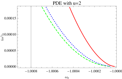
Figure 13: Plot of $\omega_{\vartheta}-\omega^{\prime}_{\vartheta}$ for PDE in LQC with $u=2$.

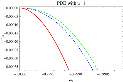
Figure 14: Plot of $\omega_{\vartheta}-\omega^{\prime}_{\vartheta}$ for PDE in LQC with $u=1$.

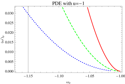
Figure 15: plot of $\omega_{\Lambda}-\omega^{\prime}_{\Lambda}$ for PDE in LQC with $u=-1$.

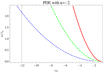
Figure 16: plot of $\omega_{\Lambda}-\omega^{\prime}_{\Lambda}$ for PDE in LQC with $u=-2$.

We also construct the $\omega_{\vartheta}-\omega^{\prime}_{\vartheta}$ plane for PDE model with different values of $u$ in LQC as shown in Figures 13-16. In all cases of $u$ and $d^{2}$, the $\omega_{\vartheta}-\omega^{\prime}_{\vartheta}$ plane corresponds to $\Lambda$CDM limit, i.e., $(\omega_{\vartheta},\omega^{\prime}_{\vartheta})=(-1,0)$. Also, $\omega_{\vartheta}-\omega^{\prime}_{\vartheta}$ plane shows thawing regions for the cases $u=2,-1,-2$ (Figures 13,15,16) and corresponds to freezing region for the case $u=1$ (Figure 14). It has been developed the following constraints on $w_{\vartheta}$ and $w^{\prime}_{\vartheta}$ by Ade et al. [49]:

$$\omega_{\vartheta} = -1.13^{+0.24}_{-0.25}~{}~{}~{}~{}~{}~{}~{}\text{(Planck+WP+BAO)},$$

$$\omega^{\prime}_{\vartheta} < 1.32,~{}~{}~{}~{}~{}~{}~{}~{}~{}~{}~{}~{}~{}~{}\text{(Planck+WP+BAO)}$$

at $95\%$ confidence level. Also, other data with different combinations of observational schemes such as (Planck+WP+Union 2.1) and (Planck+WP+SNLS) favor the above constraints. In the present case, the trajectories of $\omega^{\prime}_{\vartheta}$ against $\omega_{\vartheta}$ also meet the above mentioned values for all cases of interacting parameter which shows consistency of our results as shown in Figures 13-16. Hence, $\omega_{\vartheta}-\omega^{\prime}_{\vartheta}$ plane provides consistent behavior with the present day observations in all cases of $u$.

4.2 Statefinder Parameters

The statefinder parameters are defined as follows [53]

$$r=\frac{\dddot{a}}{aH^{3}},\quad s=\frac{r-1}{3(q-\frac{1}{2})},$$ (10)

where $q$ is the deceleration parameter. These parameters are dimensionless and possess the ability to explain the current accelerated scenario. These parameters have geometrical diagnostic due to their total dependence on the expansion factor. The statefinders are useful in the sense that we can find the distance of a given DE model from $\Lambda$CDM limit. The well-known regions described by these cosmological parameters are as follows: $(r,s)=(1,0)$ indicates $\Lambda$CDM limit, $(r,s)=(1,1)$ shows CDM limit, while $s>0$ and $r<1$ represent the region of phantom and quintessence DE eras. By following the papers [9, 10], we can obtained the following form of statefinders

$$r = 1+\frac{1}{2}a^{-3+3d^{2}}\rho_{m0}(-u^{2}n^{2}Ha^{-3+u}-(d^{4}H(a)^{-u})n^{-2}+(2u\rho_{c})(H(a)$$ (11)

$$\times (-2a^{-3+3d^{2}}\rho_{m0}+\rho_{c}-6n^{2}H(a)^{u}))^{-1})(-3-(a^{-3+3d^{2}}d^{4}\rho_{m0}H(a)^{-u})$$

$$\times n^{-2}+(a^{-3+3d^{2}}\rho_{m0}u(-un^{2}H(a)^{-2+u}+(2\rho_{c})(-2a^{-3+3d^{2}}\rho_{m0}+\rho_{c}$$

$$- 6n^{2}H(a)^{u})^{-1}))H(a)^{-1}-(3a^{3-3d^{2}}H(a)\omega^{\prime}_{\vartheta})(\rho_{m0}u(-un^{2}H(a)^{-2+u}$$

$$+ (2\rho_{c})(-2a^{-3+3d^{2}}\rho_{m0}+\rho_{c}-6n^{2}H(a)^{u})^{-1}))^{-1}).$$

and

$$s = \frac{1}{9}a^{-3+3d^{2}}\rho_{m0}(-u^{2}n^{2}H(a)^{-3+u}-(d^{4}H(a)^{-u})n^{-2}+(2u\rho_{c})(H(a)$$ (12)

$$\times (-2a^{-3+3d^{2}}\rho_{m0}+\rho_{c}-6n^{2}H(a)^{u}))^{-1})(-3-(a^{-3+3d^{2}}d^{4}\rho_{m0}H(a)^{-u})$$

$$\times n^{-2}+(a^{-3+3d^{2}}\rho_{m0}u(-un^{2}H(a)^{-2+u}+(2\rho_{c})(-2a^{(}-3+3d^{2})\rho_{m0}$$

$$+ \rho_{c}-6n^{2}H(a)^{u})^{-1}))H(a)^{-1}-(3a^{3-3d^{2}}H(a)\omega^{\prime}_{\vartheta})(\rho_{m0}u(-un^{2}H(a)^{-2+u}$$

$$+ (2\rho_{c})(-2a^{-3+3d^{2}}\rho_{m0}+\rho_{c}-6n^{2}H(a)^{u})^{-1}))^{-1}).$$

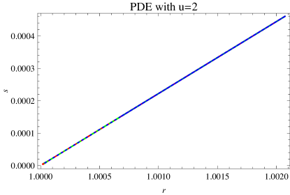
Figure 17: Plot of $r-s$ for for PDE in LQC with $u=2$.

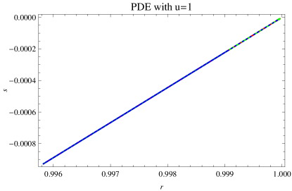
Figure 18: $r-s$ for PDE for PDE in LQC with $u=1$.

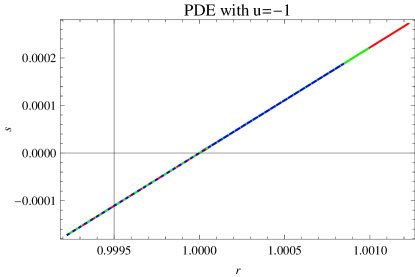
Figure 19: $r-s$ for PDE in LQC with $u=-1$.

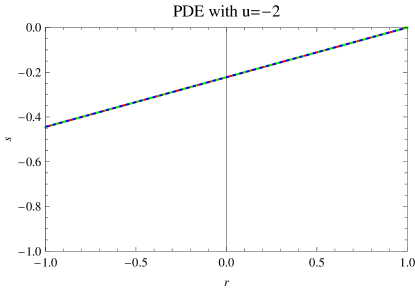
Figure 20: $r-s$ for PDE in LQC with $u=-2$.

We also develop $r-s$ planes corresponding to the present cosmological scenario for different values of $u$ as shown in Figures 17-20. The $r-s$ corresponds to $\Lambda$CDM limit for all cases of $u$.

5 Concluding Remarks

We have considered the framework of interacting PDE with Hubble horizon in LQC framework. The main motivation of this work is to analyze the cosmological scenario as well as construction of possible constraints of PDE parameter $u$ where it fulfill the PDE phenomenon. For this purpose, we have constructed Hubble parameter, EoS parameter, squared speed of sound, $\omega_{\vartheta}-\omega^{\prime}_{\vartheta}$ and $r-s$ planes, numerically. We have discussed these parameters corresponding to four values of $u=2,~{}1,-1,-2$ and three value of $d^{2}=0.2,~{}0.3,~{}0.4$. We have observed that the trajectories of Hubble parameter $H(a)$ for all cases of $u$ attains the values approximately to $74^{+0.005}_{-0.005}$ (Figures 1-4). These obtained range of $H(a)$ shows consistency with the observational values such as $H_{0}=73.8\pm 2.4$ [50] and $H_{0}=74.3\pm 1.5$ [51].

Moreover, the EoS parameter also shows consistency with the present day observations. For instance, the trajectory of $\omega_{\vartheta}$ exhibits the ranges $-1-0.0050$ and $-1+0.00005$ for the cases $u=2,~{}1$ as shown in Figures 5-6. For $u=-1,-2$ (Figures 7-8), the EoS parameter lies in the ranges $(-1.12,-1)$ and $(-5,-1)$, respectively. These constraints on EoS parameter compatible with the constraints as obtained by Ade et al. [49] (Planck data) which is given as follows:

$$\omega_{\vartheta} = -1.13^{+0.24}_{-0.25}~{}~{}~{}~{}~{}~{}~{}\text{(Planck+WP+BAO)},$$

$$\omega_{\vartheta} = -1.09\pm 0.17,~{}~{}~{}\text{(Planck+WP+Union 2.1)}$$

$$\omega_{\vartheta} = -1.13^{+0.13}_{-0.14},~{}~{}~{}~{}~{}~{}\text{(Planck+WP+SNLS)},$$

$$\omega_{\vartheta} = -1.24^{+0.18}_{-0.19},~{}~{}~{}~{}~{}~{}\text{(Planck+WP+$H_{0}$)}.$$

The above constraints has been obtained by implying different combination of observational schemes at $95\%$ confidence level.

It can also be observed from Figures 9-10 (for cases $u=2,~{}1$) that the squared speed of sound remains negative for all cases of $d^{2}$ which exhibits the instability of the PDE in LQC scenario. For the cases $u=-1,-2$ (Figures 11-12), it exhibits the stability of the present model for all cases of $d^{2}$. We have also observed that the $\omega_{\vartheta}-\omega^{\prime}_{\vartheta}$ plane corresponds to $\Lambda$CDM limit, i.e., $(\omega_{\vartheta},\omega^{\prime}_{\vartheta})=(-1,0)$ in all cases of $u$ and $d^{2}$. Also, $\omega_{\vartheta}-\omega^{\prime}_{\vartheta}$ plane shows thawing regions for the cases $u=2,-1,-2$ (Figures 13,15,16) and corresponds to freezing region for the case $u=1$ (Figure 14). It has been developed the following constraints on $w_{\vartheta}$ and $w^{\prime}_{\vartheta}$ by Ade et al. [49]:

$$\omega_{\vartheta} = -1.13^{+0.24}_{-0.25}~{}~{}~{}~{}~{}~{}~{}\text{(Planck+WP+BAO)},$$

$$\omega^{\prime}_{\vartheta} < 1.32,~{}~{}~{}~{}~{}~{}~{}~{}~{}~{}~{}~{}~{}~{}\text{(Planck+WP+BAO)}$$

at $95\%$ confidence level. Also, other data with different combinations of observational schemes such as (Planck+WP+Union 2.1) and (Planck+WP+SNLS) favor the above constraints. In the present case, the trajectories of $\omega^{\prime}_{\vartheta}$ against $\omega_{\vartheta}$ also meet the above mentioned values for all cases of interacting parameter which shows consistency of our results as shown in Figures 13-16. Hence, $\omega_{\vartheta}-\omega^{\prime}_{\vartheta}$ plane provides consistent behavior with the present day observations in all cases of $u$. Also, the $r-s$ corresponds to $\Lambda$CDM limit for all cases of $u$. Finally, it is remarked that all the cosmological parameters in the scenario of LQC with PDE shows compatibility with the current observations.

References

- [1] Perlmutter, S. et al.: Astrophys. J. 517(1999)565; Caldwell, R.R. and Doran, M.: Phys. Rev. D 69(2004)103517; Koivisto, T. and Mota, D.F.: Phys. Rev. D 73(2006)083502; Daniel, S.F.: Phys. Rev. D 77(2008)103513; Fedeli, C., Moscardini, L. and Bartelmann, M.: Astron. Astrophys. 500(2009)667.
- [2] Peebles, P.J.E.: Rev. Mod. Phys. 75(2003)559.
- [3] Kamenshchik, A.Y., Moschella, U. and Pasquier, V.: Phys. Lett. B 511(2001)265; Bento, M.C., Bertolami, O. and Sen, A.A.: Phys. Rev. D 66(2002)043507; Zhang, X., Wu, F.Q. and Zhang, J.: JCAP 01(2006)003.
- [4] Hsu, S.D.H.: Phys. Lett. B 594(2004)13.
- [5] Li, M.: Phys. Lett. B 603(2004)1.
- [6] Cai, R.G.: Phys. Lett. B 660(2008)113.
- [7] Karami, K., Ghaffari, S. and Fehri, J.: Eur. Phys. J. C 64(2009)85.
- [8] Wei, H.: Class. Quantum Grav. 29, 175008 (2012).
- [9] Sharif, M. and Jawad, A.: Eur. Phys. J. C 73, 2382 (2013).
- [10] Sharif, M. and Jawad, A.: Eur. Phys. J. C 73, 2600 (2013).
- [11] Susskind, L.: J. Math. Phys. 36(1995)6377.
- [12] Cohen, A., Kaplan, D. and Nelson, A.: Phys. Rev. Lett. 82(1999)4971.
- [13] Li, M.: Phys. Lett. B 603(2004)1.
- [14] Wei, H. and Cai, R.G.: Phys. Lett. B 660(2008)113.
- [15] Gao, C., Chen, X. and Shen, Y.G.: Phys. Rev. D 79(2009)043511; Granda, L. and Oliveros, A.: Phys. Lett. B 669(2008)275; Chen, S. and Jing, J.: Phys. Lett. B 679(2009)144.
- [16] Sharif, M. and Jawad, A.: Eur. Phys. J. Plus 129, 15 (2014); Lobo, F.S.N.: Phys. Rev. D 71(2005)124022; Lobo, F.S.N.: Phys. Rev. D 71(2005)084011;; Sushkov, S.: Phys. Rev. D 71(2005)043520.
- [17] Sharif, M. and Jawad, A.: Int. J. Mod. Phys. D 22, 1350014 (2013); Martin-Moruno, P.: Phys. Lett. B 659(2008)40; Jamil, M., Rashid, M.A. and Qadir, A.: Eur. Phys. J. C 58(2008)325; Babichev, E. et al.: Phys. Rev. D 78(2008)104027; Jamil, M.: Eur. Phys. J. C 62(2009)325; Jamil, M. and Qadir, A.: Gen. Rel. Grav. 43(2011)1069; Bhadra, J. and Debnath, U.: Eur. Phys. J. C 72(2012)1912.
- [18] Gonzalez, J.A. and Guzman, F.S.: Phys. Rev. D 79(2009)121501.
- [19] Sun, C.Y.: Commun. Theor. Phys. 52(2009)441.
- [20] Harada, T., Maeda, H. and Carr, B.J.: Phys. Rev. D 74(2006)024024; Akhoury, R., Gauthier, C.S. and Vikman, A.: JHEP 03(2009)082.
- [21] Cai, Y-F., et al.: Phys. Reports 493(2010)1.
- [22] Saridakis, E.N.: Nucl. Phys. B 819(2009)116.
- [23] Gupta, G., Saridakis, E.N. and Sen, A.A.: Phys. Rev. D 79(2009)123013.
- [24] Setare, M.R. and Saridakis, E.N.: JCAP 0903(2009)002.
- [25] Setare, M.R. and Saridakis, E.N.: Phys. Lett. B 671(2009)331.
- [26] Saridakis, E.N., Gonzalez-Diaz, P.F. and Siguenza, C.L.: Class. Quant. Grav. 26(2009)165003.
- [27] Saridakis, E.N.: Phys. Lett. B 676(2009)7.
- [28] Saridakis, E.N.: Phys. Lett. B 660(2008)138.
- [29] Saridakis, E.N.: Phys.Lett.B661:335-341,2008.
- [30] Setare, M.R. and Saridakis, E.N.: Phys. Lett. B 671(2009)331.
- [31] Sharif, M. and Rani, S.: J. Exp. Theor. Phys. (to appear, 2014).
- [32] Chattopadhyay, S., Jawad, A., Momeni, D. and Myrzakulov, R.:Astrophys. Space Sci. 353, 279 (2014).
- [33] Jawad, A.: Astrophys. Space Sci. (to appear, 2014).
- [34] Bojowald, M.: Living Rev. Rel. 8(2005)11.
- [35] Ashtekar, A., Bojowald, M. and Lewandowski, J.: Adv. Theor. Math. Phys. 7(2003)233.
- [36] Ashtekar, A.: AIP Conf. Proc. 861(2006)3.
- [37] Rovelli, C.: Living Rev. Rel. 1(1998)1.
- [38] Ashtekar, A. and Lewandowski, J.: Class. Quant. Grav. 21, R53 (2004).
- [39] Rovelli, C.: Quantum Gravity, Cambridge University Press, Cambridge (2004).
- [40] Wu, P. and Zhang, S. N., 2008, JCAP 06, 007.
- [41] Chen, S., Wang, B. and Jing, J., 2008, Phys. Rev. D 78, 123503.
- [42] Jamil, M. and Debnath, U., 2011, Astrophys Space Sci. 333, 3. [27]
- [43] Fu, X., Yu, H. and Wu, P., 2008, Phys. Rev. D 78, 063001.
- [44] Chakraborty, S., Debnath, U. and Ranjit, C.: Eur. Phys. J. C 72(2012)2101.
- [45] Pavon, D. and Zimdahl, W.: Phys. Lett. B 628(2005)206; Zimdahl, W. and Pavon, D.: Class. Quantum Grav. 24(2007)5461.
- [46] Durn, I, Pavn, D. and Zimdahlb, W.: JCAP 07(2010)018.
- [47] Gong, Y. and Li, T.: Phys. Lett. B 683(2010)241.
- [48] Sheykhi, A.: Phys. Rev. D 84(2011)107302.
- [49] Ade, P.A.R., et al.: arXiv:1303.5076.
- [50] Riess, A. G., et al.: Astrophys. J.730(2011)119.
- [51] Freedman, W. L., et al.: Astrophys. J.758(2012)24.
- [52] Caldwell, R.R. and Linder, E.V.: Phys. Rev. Lett. 95(2005)141301.
- [53] Sahni, V. et al.: JETP Lett. 77(2003)201.