Planck constraints on inflation in auxiliary vector modified $f(R)$ theories

Abstract

We show that the universal $\alpha$-attractor models of inflation can be realized by including an auxiliary vector field $A_{\mu}$ for the Starobinsky model with the Lagrangian $f(R)=R+R^{2}/(6M^{2})$. If the same procedure is applied to general modified $f(R)$ theories in which the Ricci scalar $R$ is replaced by $R+A_{\mu}A^{\mu}+\beta\nabla_{\mu}A^{\mu}$ with constant $\beta$, we obtain the Brans-Dicke theory with a scalar potential and the Brans-Dicke parameter $\omega_{\rm BD}=\beta^{2}/4$. We also place observational constraints on inflationary models based on auxiliary vector modified $f(R)$ theories from the latest Planck measurements of the Cosmic Microwave Background (CMB) anisotropies in both temperature and polarization. In the modified Starobinsky model, we find that the parameter $\beta$ is constrained to be $\beta<25$ (68 % confidence level) from the bounds of the scalar spectral index and the tensor-to-scalar ratio.

I Introduction

The inflationary paradigm Stamodel ; oldinf has been the backbone of high energy cosmology over the past three decades. For the realization of inflation, we require the existence of at least one additional degree of freedom to the Einstein-Hilbert action. A canonical scalar field with a nearly flat potential can play such a role newinf ; chaotic . In modified gravitational theories, a scalar degree of freedom generally emerges as a result of the breaking of gauge symmetries present in General Relativity Faraoni ; fRreview ; Tsujilec ; Clif .

The first model of inflation, which was proposed by Starobinsky in 1979 Stamodel , is based on the modification of gravity with the Lagrangian $f(R)=R+R^{2}/(6M^{2})$, where $R$ is the Ricci scalar and $M$ is a constant having a dimension of mass. In general, the $f(R)$ gravity is equivalent to the Brans-Dicke (BD) theory Brans with the BD parameter $\omega_{\rm BD}=0$ Ohanlon . The propagation of a scalar degree of freedom in $f(R)$ gravity is particularly transparent in the Einstein frame where a canonical scalar field $\phi$ evolves along a potential of gravitational origin conformal .

The Starobinsky model gives rise to the Einstein-frame potential with a nearly flat region responsible for inflation fRreview ; Maeda . In this model the scalar spectral index $n_{s}$ and the tensor-to-scalar ratio $r$ of primordial density perturbations generated during inflation are given, respectively, by $n_{s}\simeq 1-2/N$ and $r\simeq 12/N^{2}$, where $N$ is the number of e-foldings on scales relevant to the CMB temperature anisotropies Kofman ; Feldman ; Hwang . The Starobinsky model is consistent with the recent joint analysis of the Planck temperature data Planckcosmo and the B-mode polarization data from BICEP2/Keck array with the Planck maps at higher frequencies BKP . The tensor-to-scalar ratio is constrained to be $r<0.08$ at 95 % confidence level (CL) from such a joint analysis. The large-field models like chaotic inflation and natural inflation are now in tension with the CMB data Planckinf .

Recently, there have been numerous attempts to embed the Starobinsky model in the framework of supergravity Ketov -Ozkan or ghost-free higher-derivative gravitational theories Biswas ; Modesto . The bottom line is how to build up the Einstein-frame potential similar to the form $V(\phi)=V_{0}(1-e^{-\sqrt{2/3}\,\phi/M_{\rm pl}})^{2}$, where $M_{\rm pl}=2.435\times 10^{18}$ GeV is the reduced Planck mass. In a particular version of supergravity where the inflaton is a part of a vector multiplet it is possible to construct a generalized potential of the form $V(\phi)=V_{0}(1-e^{-\sqrt{2/(3\alpha)}\,\phi/M_{\rm pl}})^{2}$, where the parameter $\alpha$ is inversely proportional to the curvature of the inflaton Kähler manifold KLR . This was dubbed the $\alpha$-attractor model in which the inflationary period is followed by the reheating stage with the inflaton oscillations around $\phi=0$.

In the limit $\alpha\to\infty$ the potential of the $\alpha$-attractor model is approximately given by $V(\phi)\propto\phi^{2}$, so it is equivalent to that of the quadratic potential in chaotic inflation chaotic . For $1\leq\alpha<\infty$ the tensor-to-scalar ratio is in the range $O(10^{-3})<r<O(10^{-1})$, with $n_{s}$ inside the 95 % CL observational contour constrained by the Planck data Planck1 ; Kuro ; Planckinf . In Ref. Tavakol the authors derived the same potential as that of the $\alpha$-attractor model by generalizing the Starobinsky model in the framework of the BD theory and they placed observational constraints on the model from the WMAP 7yr data.

In this paper we show that the $\alpha$-attractor model arises by introducing an auxiliary vector field $A_{\mu}$ and replacing the Ricci scalar $R$ with $R+A_{\mu}A^{\mu}+\beta\nabla_{\mu}A^{\mu}$ in the Starobinsky Lagrangian, where $\nabla_{\mu}$ is the covariant derivative. This procedure can be extended to the general $f(R)$ Lagrangian. The resulting theory is equivalent to the BD theory characterized by the BD parameter $\omega_{\rm BD}=\beta^{2}/4$ with one scalar propagating degree of freedom.

In light of the recent release of the Planck temperature and polarization data, we also put observational constraints on inflationary models in the framework of auxiliary vector modified $f(R)$ theories. Our analysis not only encompasses the $\alpha$-attractor model but also the models derived by promoting the Lagrangian $f(R)=R+cR^{n}$ ($n>1$) to include the auxiliary vector field. This can accommodate a wider class of inflationary models including chaotic inflation with the potential $V(\phi)\propto\phi^{n/(n-1)}$.

This paper is organized as follows. In Sec. II we review the Starobinsky model and its dual description in terms of a scalar degree of freedom $\phi$. In Sec. III we show how the $\alpha$-attractor model emerges by modifying the Starobinsky model with inclusion of the auxiliary vector field. In Sec. IV we extend this prescription to general $f(R)$ theories and provide the formulas of inflationary observables associated with the primordial scalar and tensor perturbations. In Sec. V we place observational bounds on the auxiliary vector modified inflationary models from the latest Planck data combined with other B-mode polarization data. Sec. VI is devoted to conclusions.

II Starobinsky model and its dual description

The Starobinsky model Stamodel is described by the action

$$S=\frac{M_{\rm pl}^{2}}{2}\int d^{4}x\sqrt{-g}\,{\cal L}(R)\,,$$ (1)

where $g$ is the determinant of the space-time metric $g_{\mu\nu}$ and ${\cal L}(R)$ is a function of $R$ of the form

$${\cal L}(R)=R+\frac{R^{2}}{6M^{2}}\,.$$ (2)

The discussion given below is already well known in the literature fRreview , but this is useful for the comparison with the auxiliary modified Starobinsky model given in Sec. III. The model (2) possesses an additional scalar degree of freedom to that in General Relativity. In order to make this manifest, we consider the following Lagrangian

$$\mathcal{L}=F+\frac{F^{2}}{6M^{2}}-\varphi(F-R)\,.$$ (3)

It is easy to see that, upon integrating out the field $\varphi$, we get back to the original Starobinsky model (1). Varying Eq. (3) with respect to $F$, it follows that

$$F=3M^{2}(\varphi-1)\,.$$ (4)

Then, the Lagrangian (3) can be rewritten as

$$\mathcal{L}=\varphi R-\frac{3}{2}M^{2}(\varphi-1)^{2}\,.$$ (5)

This is equivalent to the BD theory Brans with the BD parameter $\omega_{\rm BD}=0$ and the scalar potential $V(\varphi)=(3/2)M^{2}(\varphi-1)^{2}$.

In Eq. (5) the scalar degree of freedom $\varphi$ is directly coupled to the Ricci scalar $R$. One can transform the action (1) with the Lagrangian (5) to the so-called Einstein frame under the conformal transformation $\widetilde{g}_{\mu\nu}=\Omega^{2}(\varphi)g_{\mu\nu}$ conformal . Denoting the quantities in the transformed frame as a tilde, we have the following relations fRreview

$$\sqrt{-g} = \Omega^{-4}\sqrt{-\widetilde{g}}\,,$$ (6)

$$R = \Omega^{2}(\widetilde{R}+6\widetilde{\Box}\omega-6\widetilde{g}^{\mu\nu}\nabla_{\mu}\omega\nabla_{\nu}\omega)\,,$$ (7)

where $\omega\equiv\ln\Omega$. We obtain the Einstein-frame action for the choice

$$\Omega^{2}=\varphi\,,$$ (8)

under which the Ricci scalar $\widetilde{R}$ does not have a direct coupling with $\varphi$. Dropping the total derivative term $\widetilde{\Box}\omega$ in Eq. (7) and introducing a scalar field

$$\phi\equiv\sqrt{\frac{3}{2}}M_{\rm pl}\,\ln\varphi\,,$$ (9)

the action in the Einstein frame reads

$$S=\int d^{4}x\sqrt{-\widetilde{g}}\left[\frac{M_{\rm pl}^{2}}{2}\widetilde{R}-\frac{1}{2}\widetilde{g}^{\mu\nu}\nabla_{\mu}\phi\nabla_{\nu}\phi-V(\phi)\right]\,,$$ (10)

where

$$V(\phi)=\frac{3}{4}M_{\rm pl}^{2}M^{2}\left(1-e^{-\sqrt{\frac{2}{3}}\frac{\phi}{M_{\rm pl}}}\right)^{2}\,.$$ (11)

Hence the scalar degree of freedom $\phi$, which is the gravitational origin, propagates with the kinetic energy $-(1/2)\widetilde{g}^{\mu\nu}\nabla_{\mu}\phi\nabla_{\nu}\phi$. The potential (11) is sufficiently flat for $\phi$ larger than the order of $M_{\rm pl}$, in which regime inflation occurs due to the slow-roll evolution of $\phi$.

III Auxiliary Modified Starobinsky Model

The auxiliary vector modified Starobinsky model is inspired by the supersymmetric extension of Starobinsky model Ketov -Ozkan . In the old minimal formulation of ${\cal N}=1$ off-shell supergravity, the Weyl multiplet consists of the vielbein $e^{a}_{\mu}$, the gravitino $\psi^{a}_{\mu}$, an auxiliary vector $A_{\mu}$ and an auxiliary complex scalar $S$. The embedding of Starobinsky model in the old minimal supergravity is obtained by coupling a chiral multiplet to the Weyl multiplet. The supersymmetric Starobinsky model can be recast into the form of a scalar-tensor theory by integrating out the auxiliary fields. In particular, integrating out the auxiliary vector field generates the kinetic term for the imaginary part of the complex scalar in the chiral multiplet.

We apply the similar mechanism here by coupling an auxiliary vector field to the Starobinsky model in a specific way such that the auxiliary vector field does not generate new degrees of freedom. As we will show below, integrating out the auxiliary vector field modifies the kinetic term of inflaton. The resulting theory written in the Einstein frame coincides with the $\alpha$-attractor model proposed in Ref. KLR . In analogous to the supersymmetric extension of Starobinsky model, the auxiliary vector modified Starobinsky model thus provides a gravitational origin for the designed scalar potential in the $\alpha$-attractor model. We can also apply the same mechanism to auxiliary vector coupled $f(R)$ theories and obtain a class of generalized $\alpha$-attractor models (see Sec. IV.1).

We would like to stress that our model is inspired by the ${\cal N}=1$ off-shell supergravity, but it does not directly come from a supersymmetric scenario with a SUSY breaking mechanism. Hence we do not take into account the effect of gravitinos for the cosmological dynamics. Construction of a SUSY breaking $\alpha$-attractor model with the effect of gravitinos taken into account is beyond the scope of our paper.

We start with the Lagrangian of the form ${\cal L}=R+A_{\mu}A^{\mu}+\beta\nabla_{\mu}A^{\mu}$, where $\beta$ is a constant. Note that the coefficient in front of the term $A_{\mu}A^{\mu}$ has been fixed to 1. When higher derivative terms are included, $A_{\mu}$ can pick up kinetic terms such as $(\nabla_{\mu}A^{\mu})^{2}$ and $F_{\mu\nu}F^{\mu\nu}$, so the auxiliary vector starts to propagate. If we would like to allow kinetic terms for $A_{\mu}$ but still wish to keep $A_{\mu}$ as an auxiliary vector in the higher derivative extended model, then the action of the auxiliary vector modified Starobinsky model has to take the following form:

$$S=\frac{M_{\rm pl}^{2}}{2}\int d^{4}x\sqrt{-g}\,{\cal L}\,,$$ (12)

where

$$\mathcal{L} = R+A_{\mu}A^{\mu}+\beta\nabla_{\mu}A^{\mu}$$ (13)

$$+\frac{1}{6M^{2}}\Big{(}R+A_{\mu}A^{\mu}+\beta\nabla_{\mu}A^{\mu}\Big{)}^{2}\,.$$

In order to see that this model gives rise to only one scalar degree of freedom, we perform the similar analysis to that performed in the previous section. We first write Eq. (13) as

$$\mathcal{L}=F+\frac{1}{6M^{2}}F^{2}-\varphi\Big{(}F-R-A_{\mu}A^{\mu}-\beta\nabla_{\mu}A^{\mu}\Big{)}\,.$$ (14)

Varying the Lagrangian (14) with respect to $A^{\mu}$ and $F$, respectively, it follows that

$$A_{\mu} = \frac{1}{2\varphi}\beta\nabla_{\mu}\varphi\,,$$ (15)

$$F = 3M^{2}(\varphi-1)\,.$$ (16)

The equation of motion (15) of the auxiliary vector field demonstrates that on-shell, the vector field is equivalent to the gradient of the scalar field. Therefore, there are no dynamical spin-1 degrees of freedom in our model. Consequently, the apparent presence of a vector field in our model does not spoil the homogeneity and isotropy of the universe.

Substituting the relations (15)-(16) into Eq. (14) and dropping a total derivative term, we obtain the (Jordan-frame) Lagrangian

$$\mathcal{L}=\varphi R-\frac{1}{4\varphi}\beta^{2}\nabla_{\mu}\varphi\nabla^{\mu}\varphi-\frac{3}{2}M^{2}(\varphi-1)^{2}\,.$$ (17)

This theory is equivalent to the BD theory with the BD parameter

$$\omega_{\rm BD}=\frac{1}{4}\beta^{2}\,,$$ (18)

so the auxiliary vector model (13) possesses one scalar degree of freedom.

Under the conformal transformation $\widetilde{g}_{\mu\nu}=\Omega^{2}(\varphi)g_{\mu\nu}$ with $\Omega^{2}=\varphi$, the action in the Einstein frame reads

$$S=\int d^{4}x\sqrt{-\widetilde{g}}\left[\frac{M_{\rm pl}^{2}}{2}\widetilde{R}-\frac{1}{2}\widetilde{g}^{\mu\nu}\nabla_{\mu}\phi\nabla_{\nu}\phi-V(\phi)\right]\,,$$ (19)

where $\phi$ is a canonical scalar field defined by

$$\phi=\frac{\sqrt{6+\beta^{2}}}{2}M_{\rm pl}\ln\varphi\,.$$ (20)

The potential $V(\phi)$ is given by

$$V(\phi)=\frac{3}{4}M_{\rm pl}^{2}M^{2}\left(1-e^{-\sqrt{\frac{2}{3\alpha}}\frac{\phi}{M_{\rm pl}}}\right)^{2}\,,$$ (21)

where

$$\alpha\equiv 1+\frac{\beta^{2}}{6}=1+\frac{2}{3}\omega_{\rm BD}\,.$$ (22)

This is equivalent to the $\alpha$-attractor model studied in Ref. KLR . Setting $\beta=0$, we recover the Starobinsky model described by the potential (11) in the Einstein frame.

Figure 1: Evolution of the scalar field $\phi$ and the Hubble parameter $\tilde{H}$ in the Einstein frame for $\beta=10$. We choose the initial conditions $\phi=10M_{\rm pl}$ and $\dot{\phi}=0$ at $\tilde{t}=0$. In this case the inflationary period lasts with the number of e-foldings about 55, which is followed by the reheating stage with the oscillating inflaton field.

Around $\phi=0$, the potential (21) is approximately given by $V(\phi)\simeq M^{2}\phi^{2}/(2\alpha)$. The graceful exit from inflation to reheating naturally occurs after the field $\phi$ enters the regime $\sqrt{2/(3\alpha)}\phi/M_{\rm pl}\ll 1$. In Fig. 1 we plot the evolution of the field $\phi$ and the Hubble parameter $\tilde{H}$ versus the cosmic time $\tilde{t}$ in the Einstein frame for $\beta=10$. During inflation, the field evolves slowly along the potential (21) with a nearly constant Hubble parameter. For the parameter $\beta$ and initial conditions chosen in Fig. 1, the end of inflation is characterized by the field value $\phi_{f}\simeq 0.8M_{\rm pl}$ with the number of e-foldings $N\simeq 55$. This shows good agreement with the analytic estimation given in Sec. V.1 [see Eq. (39)].

As we see in Fig. 1, the Universe exits from the inflationary epoch to the reheating stage driven by the oscillation of $\phi$. The field $\phi$ exhibits a damped oscillation around the potential minimum at $\phi=0$. Since the auxiliary vector only gives rise to the change of the kinetic term of $\varphi$ in Eq. (17), it does not modify the cosmological dynamics after the field $\phi$ stabilizes at the minimum of the Einstein-frame potential (21), i.e., after reheating. In Appendix A we estimate the time at the onset of radiation-dominated era. After this epoch, the energy density of radiation dominates over that of $\phi$.

Since the field $\phi$ behaves as a massive oscillating scalar around the potential minimum, the basic mechanism of reheating is similar to that in the Starobinsky model reheating ; reheating2 ; fRreview apart from the fact that the energy scale of the potential gets lowered by the factor $1/\alpha$. The modified kinetic term in the Jordan frame can be interpreted as the modified shape of the potential in the Einstein frame. As we will see in Sec. V.1, this modification of the Einstein-frame potential gives rise to the change of CMB observables relative to those in the Starobinsky model. Especially, the larger value of the tensor-to-scalar ratio $r$ caused by the modification of the kinetic term of $\varphi$ is a distinguished observational feature to discriminate between the $\alpha$-attractor model [$O(10^{-3})<r<O(10^{-1})$] and the Starobinsky model [$r=O(10^{-3})$].

The observational constraints on the potential (21) were discussed in Ref. Tavakol with the WMAP 7yr data and in Ref. KLR with the Planck 1yr data. In Sec. V we shall place observational bounds on the same model as well as more general models from the latest Planck temperature data combined with other data.

IV Auxiliary vector modified $f(R)$ theories and inflationary observables

The discussion in Sec. III can be extended to more general auxiliary vector modified $f(R)$ theories. In this section we shall perform such an analysis and then provide the formulas of the primordial power spectra of scalar and tensor perturbations generated during inflation.

IV.1 Auxiliary vector modified $f(R)$ theories

The auxiliary vector modification to $f(R)$ theories requires replacing $R$ with $R+A_{\mu}A^{\mu}+\beta\nabla_{\mu}A^{\mu}$. Thus the model is given by the action (12) with

$$\mathcal{L}=f(R+A_{\mu}A^{\mu}+\beta\nabla_{\mu}A^{\mu})\,.$$ (23)

We rewrite this Lagrangian of the following form

$$\mathcal{L}=f(F)-\varphi(F-R-A_{\mu}A^{\mu}-\beta\nabla_{\mu}A^{\mu})\,.$$ (24)

Varying Eq. (24) with respect to $A^{\mu}$ and $F$, we obtain

$$A_{\mu} = \frac{1}{2\varphi}\beta\nabla_{\mu}\varphi\,,$$ (25)

$$f_{,F}(F) = \varphi\,.$$ (26)

Here and in the following, a comma in the lower index denotes the partial derivatives with respect to scalar quantities represented in the index, e.g., $f_{,F}\equiv\partial f/\partial F$. The quantity $F$ depends on $\varphi$ through the relation (26).

Substituting Eq. (25) into Eq. (24), it follows that

$$\mathcal{L}=\varphi R-\frac{1}{4\varphi}\beta^{2}\nabla_{\mu}\varphi\nabla^{\mu}\varphi-\left[\varphi F(\varphi)-f(F(\varphi))\right]\,.$$ (27)

This is equivalent to the BD theory with the same BD parameter as Eq. (18). Compared to Eq. (17), the scalar potential in the Jordan frame is generalized to $V_{J}(\varphi)=\varphi F(\varphi)-f(F(\varphi))$.

Introducing the scalar field $\phi$ as Eq. (20) and carrying out the conformal transformation $\widetilde{g}_{\mu\nu}=\varphi\,g_{\mu\nu}$, we obtain the Einstein-frame action (19) with the scalar potential

$$V(\phi)=\frac{M_{\rm pl}^{2}}{2}e^{-\sqrt{\frac{2}{3\alpha}}\frac{\phi}{M_{\rm pl}}}\left[F-e^{-\sqrt{\frac{2}{3\alpha}}\frac{\phi}{M_{\rm pl}}}f(F)\right]\,,$$ (28)

where $f_{,F}(F)=\varphi=e^{\sqrt{\frac{2}{3\alpha}}\frac{\phi}{M_{\rm pl}}}$. The $\alpha$-attractor model, which corresponds to the potential (21), is a special case of a larger class of auxiliary vector modified $f(R)$ theories. When $\beta=0$ we have $A_{\mu}=0$ from Eq. (25), so that the Lagrangian (23) recovers that of $f(R)$ theories.

IV.2 Inflationary observables

Let us study inflation for the theories described by the action (12) with the Lagrangian (23). We assume that the background is described by the flat Friedmann-Lemaître-Robertson-Walker metric with the line element $ds^{2}=-dt^{2}+a^{2}(t)\delta_{ij}dx^{i}dx^{j}$, where the scale factor $a(t)$ depends on the cosmic time $t$. We consider scalar and tensor metric perturbations on this background.

In the Einstein frame the action is given by Eq. (19) with the potential (28). In Refs. Fakir it was shown that the inflationary observables associated with linear scalar and tensor perturbations are invariant under the conformal transformation.

The spectral index of scalar perturbations with the primordial power spectrum ${\cal P}_{s}$ is defined by $n_{s}\equiv 1+d\ln{\cal P}_{s}/d\ln k$, where $k$ is a comoving wavenumber. We also introduce the tensor-to-scalar ratio, as $r\equiv{\cal P}_{h}/{\cal P}_{s}$, where ${\cal P}_{h}$ is the primordial power spectrum of tensor perturbations. Under the slow-roll approximation during inflation, these observables are given by infreview

$${\cal P}_{s} = \frac{V^{3}}{12\pi^{2}M_{\rm pl}^{6}V_{,\phi}^{2}}\,,$$ (29)

$$n_{s} = 1-6\epsilon+2\eta\,,$$ (30)

$$r = 16\epsilon\,,$$ (31)

where

$$\epsilon\equiv\frac{M_{\rm pl}^{2}}{2}\left(\frac{V_{,\phi}}{V}\right)^{2}\,,\qquad\eta\equiv\frac{M_{\rm pl}^{2}V_{,\phi\phi}}{V}\,.$$ (32)

As long as the slow-roll condition is satisfied, the analytic estimations (29)-(31) are accurate enough to confront inflationary models with the CMB observations. Defining the tensor spectral index as $n_{t}\equiv d\ln{\cal P}_{h}/d\ln k$, the following consistency relation holds infreview

$$r=-8n_{t}\,.$$ (33)

We define the number of e-foldings $N=\ln[a(t_{f})/a(t)]$ in the Jordan frame, where $a(t)$ and $a(t_{f})$ are the scale factors at the moments $t$ and $t_{f}$ respectively. The lower index “$f$” represents the values at the end of inflation. We identify the field value $\phi_{f}$ by the condition $\epsilon(\phi_{f})=1$.

The number of e-foldings is a frame-independent quantity by properly choosing the observer’s reference frame Catena . On using the relations $\widetilde{a}=\Omega a$ and $d\tilde{t}=\Omega dt$ conformal ; Maeda , the Hubble parameters $\widetilde{H}=(d\widetilde{a}/d\tilde{t})/\widetilde{a}$ and $H=(da/dt)/a$ in the two frames are related with each other as $\widetilde{H}=[H+(d\Omega/dt)/\Omega]/\Omega$. Since we are considering the choice (8), the number of e-foldings $N=\int_{t}^{t_{f}}Hdt$ can be expressed as $N=\int_{\tilde{t}}^{\tilde{t}_{f}}\widetilde{H}d\tilde{t}+\ln(\varphi/\varphi_{f})^{1/2}$. On using the slow-roll approximations $3M_{\rm pl}^{2}\widetilde{H}^{2}\simeq V$ and $3\widetilde{H}d\phi/d\tilde{t}\simeq-V_{,\phi}$ in the Einstein frame, it follows that

$$N=\int_{\phi_{f}}^{\phi}\frac{V}{M_{\rm pl}^{2}V_{,\phi}}d\phi+\frac{1}{\sqrt{6\alpha}}\frac{\phi-\phi_{f}}{M_{\rm pl}}\,.$$ (34)

The number of e-foldings associated with the CMB temperature anisotropies corresponds to $50\lesssim N\lesssim 60$ infreview . On using Eq. (34), the inflationary observables (30) and (31) can be known as functions of $N$.

V Observational constraints from the latest CMB data

We put observational constraints on several different inflationary models that belong to the class of auxiliary vector modified $f(R)$ theories.

We employ the bounds in the $(n_{s},r)$ plane derived by the latest Planck CMB temperature data (Temperature-Temperature (TT), Temperature-E-mode (TE), E-mode-E-mode (EE) correlation power spectra) and a first release of the B-mode polarization data Planckcosmo . The Planck mission also performed the joint analysis by taking into account the B-mode maps from BICEP2 and Keck Array with the Planck maps (BKP) at higher frequencies where the emission of dust dominates BKP . This study showed that there is no statistical significant evidence for the detection of primordial gravitational waves. Still, the latest BKP analysis put tighter upper bounds on the tensor-to-scalar ratio $r$ than those derived by the Planck data alone Planckinf .

The likelihood analysis of the Planck mission is based on expansions of the scalar and power spectra of the forms ${\cal P}_{s}(k)=A_{s}(k/k_{*})^{n_{s}-1+(\alpha_{s}/2)\ln(k/k_{*})+\cdots}$ and ${\cal P}_{h}(k)=A_{t}(k/k_{*})^{n_{t}+(\alpha_{t}/2)\ln(k/k_{*})+\cdots}$, respectively, where $\alpha_{s,t}=dn_{s,t}/d\ln k$ are the runnings of the spectral indices and $k_{*}$ is the pivot wavenumber. Since there is no significant evidence for the large deviation of $\alpha_{s,t}$ from 0, the standard slow-roll prediction of inflationary observables is consistent with the CMB data.

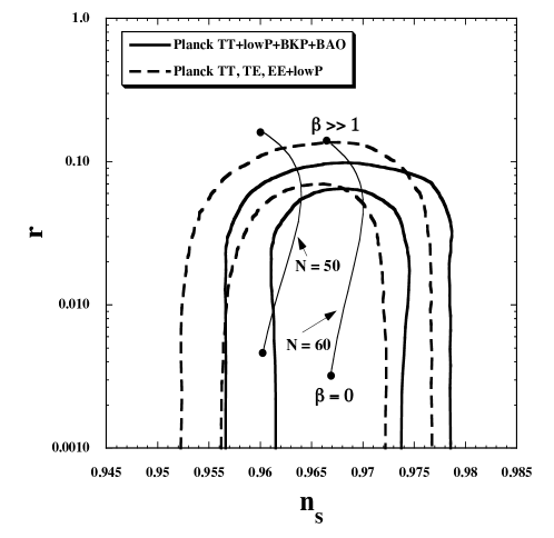
Figure 2: The 68 % CL (inside) and 95 % CL (outside) observational contours in the $(n_{s},r)$ plane derived from the joint data analysis of Planck TT+lowP+BKP+BAO (thick solid) and Planck TT, TE, EE+lowP (thick dashed). The pivot scale is chosen to be $k_{*}=0.002$ Mpc^-1. We also show the theoretical curves of the auxiliary vector modified Starobinsky model (13) as functions of $\beta$ for $N=50$ and $60$ (thin solid).

In Fig. 2 we show the 68 % CL and 95 % CL observational contours in the $(n_{s},r)$ plane derived by the latest Planck temperature data as well as the BKP and Baryon Acoustic Oscillations (BAO) data. From the Planck TT, TE, EE and low-multipole temperature polarization data (denoted as “lowP”), the tensor-to-scalar ratio $r$ is constrained to be $r<0.15$ (95 % CL) Planckinf . Combination of the BKP cross-correlation with the Planck TT+lowP data gives a tighter bound $r<0.08$ (95 % CL). Inclusion of the BAO data leads to the shift of $n_{s}$ toward larger values (as in the figure 1 of Ref. Kuro ). In the following we shall place observational constraints on concrete auxiliary vector modified $f(R)$ models.

V.1 Auxiliary vector modified Starobinsky model

Let us begin with the model (13), i.e.,

$$f(F)=F+\frac{F^{2}}{6M^{2}}\,,$$ (35)

in the Lagrangian (24). Since the potential in the Einstein frame is given by Eq. (21), the observables (29)-(31) reduce to

$${\cal P}_{s} = \frac{3\alpha}{128\pi^{2}}\left(\frac{M}{M_{\rm pl}}\right)^{2}\frac{(1-x)^{4}}{x^{2}}\,,$$ (36)

$$n_{s} = 1-\frac{8x(x+1)}{3\alpha(1-x)^{2}}\,,$$ (37)

$$r = \frac{64x^{2}}{3\alpha(1-x)^{2}}\,,$$ (38)

where $x\equiv e^{-\sqrt{2/(3\alpha)}\phi/M_{\rm pl}}$. The number of e-foldings (34) reads

$$N=\frac{3}{4}\alpha\left(\frac{1}{x}-\frac{1}{x_{f}}\right)+\left(\frac{3}{4}\alpha-\frac{1}{2}\right)\ln\left(\frac{x}{x_{f}}\right)\,,$$ (39)

where $x_{f}=(2\sqrt{3\alpha}-3\alpha)/(4-3\alpha)$.

When the parameter $\alpha=1+\beta^{2}/6$ is of the order of 1, the inflationary epoch corresponds to the regime in which $\phi$ is larger than $M_{\rm pl}$, i.e., $x\ll 1$. Since $N\simeq 3\alpha/(4x)$ in this case, it follows that

$${\cal P}_{s}\simeq\frac{N^{2}M^{2}}{24\pi^{2}\alpha M_{\rm pl}^{2}}\,,\qquad n_{s}\simeq 1-\frac{2}{N}\,,\qquad r\simeq\frac{12\alpha}{N^{2}}\,.$$ (40)

From the Planck normalization ${\cal P}_{s}\simeq 2.2\times 10^{-9}$ Planckcosmo , the mass scale $M$ is constrained to be

$$\frac{M}{M_{\rm pl}}\simeq 1.3\times 10^{-5}\sqrt{\alpha}\left(\frac{N}{55}\right)^{-1}\qquad{\rm for}\leavevmode\nobreak\ \leavevmode\nobreak\ \alpha=O(1)\,.$$ (41)

In the presence of the coupling $\beta$, both $M$ and $r$ are larger than those in the the Starobinsky $f(R)$ model ($\alpha=1$).

In the limit that $\alpha\gg 1$, inflation occurs in the region around $x=1$, so the potential (21) reduces to $V(\phi)\simeq M^{2}\phi^{2}/(2\alpha)$. This means that, for increasing $\beta$, the observables (37) and (38) approach the values of the quadratic potential, i.e., $n_{s}\simeq 1-2/N$ and $r\simeq 8/N$. Since the scalar power spectrum is given by ${\cal P}_{s}\simeq N^{2}M^{2}/(6\pi^{2}\alpha M_{\rm pl}^{2})$, the Planck normalization gives

$$\frac{M}{M_{\rm pl}}\simeq 6.6\times 10^{-6}\sqrt{\alpha}\left(\frac{N}{55}\right)^{-1}\qquad{\rm for}\leavevmode\nobreak\ \leavevmode\nobreak\ \alpha\gg 1\,.$$ (42)

In this regime the mass scale $M$ is higher than that for $\alpha=O(1)$.

In Fig. 2 we plot the theoretical curves in the $(n_{s},r)$ plane as functions of $\beta$ (ranging $0\leq\beta\leq 10^{6}$) for $N=50$ and $60$. The quadratic potential is outside the 95 % CL observational contours. For $N=60$ the joint data analysis of Planck TT+lowP+BKP+BAO gives the following bounds

$$\beta<25\qquad(68\,\%\,{\rm CL})\,,$$ (43)

$$\beta<66\qquad(95\,\%\,{\rm CL})\,.$$ (44)

For $N=50$ the Starobinsky model ($\beta=0$) is outside the 68 % CL region (mainly due to inclusion of the BAO data), but it is still inside the 68% CL contour constrained by Planck TT, TE, EE+lowP.

V.2 Power-law model

We proceed to the power-law model given by

$$f(F)=m^{2(1-n)}F^{n}\,,$$ (45)

where $m$ and $n$ are positive constants. Since $F^{n-1}=\varphi/(nm^{2(1-n)})$ from Eq. (26), the Einstein-frame potential (28) reduces to

$$V(\phi)=\frac{n-1}{2n^{n/(n-1)}}M_{\rm pl}^{2}m^{2}\exp\left(-\frac{n-2}{n-1}\sqrt{\frac{2}{3\alpha}}\frac{\phi}{M_{\rm pl}}\right)\,.$$ (46)

The positivity of the potential requires the condition $n>1$. The power-law inflation ($a\propto t^{p}$ with $p>1$) powerlaw can be realized for $3\alpha>[(n-2)/(n-1)]^{2}$. In this case we have

$$n_{s} = 1-\frac{2(n-2)^{2}}{3\alpha(n-1)^{2}}\,,$$ (47)

$$r = 8(1-n_{s})\,.$$ (48)

The Harrison-Zeldovich spectrum corresponds to the limit $n\to 2$ or $\alpha\to\infty$.

The theoretical values of $n_{s}$ and $r$ are on the line (48) in the $(n_{s},r)$ plane. This line is outside the 95 % CL regions shown in Fig. 2, so the power-law model (45) is disfavored from the data.

V.3 Generalization of the auxiliary vector modified Starobinsky model

Finally we study the following model

$$f(F)=F+m^{2(1-n)}F^{n}\,,$$ (49)

where $m$ and $n\leavevmode\nobreak\ (\neq 2)$ are positive constants. In this case the potential in the Einstein frame is given by

$$V(\phi)=\frac{n-1}{2n^{n/(n-1)}}M_{\rm pl}^{2}m^{2}e^{-2\sqrt{\frac{2}{3\alpha}}\frac{\phi}{M_{\rm pl}}}\left(e^{\sqrt{\frac{2}{3\alpha}}\frac{\phi}{M_{\rm pl}}}-1\right)^{\frac{n}{n-1}}\,.$$ (50)

Since we consider inflation in the regime $\phi>0$, the positivity of the potential requires that $n>1$.

For given $n$ and $\beta$, we numerically compute the field value $\phi_{f}$ at the end of inflation according to the condition $\epsilon(\phi_{f})=1$. From Eq. (34) we identify the field value $\phi$ corresponding to $N=60$ and then evaluate the observables (30) and (31).

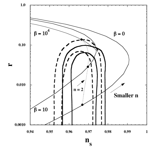
Figure 3: The theoretical curves of the model (49) with $N=60$ in the $(n_{s},r)$ plane for $\beta=0,10,10^{4}$. These curves are plotted as as functions of the power $n\leavevmode\nobreak\ (>1)$. The theoretical prediction for the $n=2$ case is shown as a thin dotted curve. For smaller $n$, the tensor-to-scalar ratio gets larger. The 68 % CL and 95 % CL observational contours are the same as those plotted in Fig. 2.

Let us first discuss the case $\beta=0$. Since inflation occurs in the regime where $\phi$ is bigger than $M_{\rm pl}$, the large deviation of the power $n$ from 2 spoils the flatness of the potential. In Fig. 3 we plot the theoretical curve in the $(n_{s},r)$ plane for $N=60$ as a function of $n$. The Starobinsky model ($n=2$) is shown as a black circle. For smaller $n$ the tensor-to-scalar ratio gets larger, whereas the scalar spectral index reaches a maximum value $n_{s}=0.991$ around $n=1.92$ and then turns into decrease. When $n>2$, the inflationary observables are particularly sensitive to the deviation from $n=2$ because of the appearance of the potential maximum in the Einstein frame. From the Planck TT+lowP+BKP+BAO joint analysis we obtain the following bound

$$1.980<n<2.015\qquad(\beta=0)\,,$$ (51)

at 95 % CL. Hence only the tiny deviation from $n=2$ is allowed for the consistency with the CMB data. The mass scale $m$ constrained by the Planck normalization is similar to that given in Eq. (41), with the correspondence $m=\sqrt{6}M$ and $\alpha=1$.

In Fig. 3 we also plot the theoretical curve for $\beta=10$ as a function of $n$. The qualitative behavior of $n_{s}$ and $r$ with respect to the change of $n$ is similar to that for $\beta=0$. The Planck TT+lowP+BKP+BAO joint analysis gives the bound

$$1.75<n<2.39\qquad(\beta=10)\,,$$ (52)

at 95 % CL. The wider range of $n$ is allowed relative to the case $\beta=0$. This reflects the fact that, for larger $\beta$, inflation can occur in the regime where the quantity $x=e^{-\sqrt{2/(3\alpha)}\phi/M_{\rm pl}}$ is not very much smaller than 1. When $\beta=10$, for example, the order of $x$ satisfying the bound (52) is typically 0.1 at $N=60$, whereas, for $\beta=0$, $x$ is of the order of $0.01$ for $n$ ranging in Eq. (51).

In the limit $\beta\to\infty$ the epoch of inflation corresponds to the regime $x\simeq 1$ and hence the potential (50) can be approximated as

$$V(\phi)\simeq\frac{n-1}{2n^{p}}\left(\frac{2}{3\alpha}\right)^{p/2}M_{\rm pl}^{2}m^{2}\left(\frac{\phi}{M_{\rm pl}}\right)^{p}\,,$$ (53)

where

$$p\equiv\frac{n}{n-1}\,.$$ (54)

This is equivalent to chaotic inflation with the power-law potential $V(\phi)\propto\phi^{p}$, so the inflationary observables are estimated as

$${\cal P}_{s} \simeq \frac{c_{n}}{12\pi^{2}p^{2}}\left(\frac{m}{M_{\rm pl}}\right)^{2}\left(\frac{\phi}{M_{\rm pl}}\right)^{p+2}\,,$$ (55)

$$n_{s} \simeq 1-\frac{p+2}{2N}\,,$$ (56)

$$r \simeq \frac{4p}{N}\,,$$ (57)

where $c_{n}\equiv(n-1)[2/(3\alpha)]^{p/2}/(2n^{p})$. In the limits $n\to 1$ and $n\to\infty$ we have $p\to\infty$ and $p\to 1$, respectively. On using the relation $\phi/M_{\rm pl}\simeq(2pN)^{1/2}$, the Planck normalization constrains the mass scale $m$, as

$$\frac{m}{M_{\rm pl}}\simeq 5.1\times 10^{-4}\,p\,c_{n}^{-1/2}\,(2pN)^{-(p+2)/4}\,.$$ (58)

In Fig. 3 we plot the theoretical curve for $\beta=10^{4}$ in the range $1.2\leq n\leq 100$. The values of $n_{s}$ and $r$ are very close to those estimated from Eqs. (56) and (57). Provided that $n>3.5$, the models are inside the 95 % CL region constrained by the Planck TT+lowP+BKP+BAO data. However, even the linear potential $V(\phi)\propto\phi$ (i.e., $n\to\infty$) is marginally inside the 95 % CL contour, so the models with $\beta\gg 1$ are not generally favored from the CMB data.

VI Conclusions

In this paper we showed that the auxiliary vector modification to the Starobinsky model derived by replacing $R$ with $R+A_{\mu}A^{\mu}+\beta\nabla_{\mu}A^{\mu}$ gives rise to the universal $\alpha$-attractor model proposed in the context of supergravity. Applying the same prescription to general $f(R)$ theories, the resulting action is equivalent to that of BD theories with the BD parameter $\omega_{\rm BD}=\beta^{2}/4$. Under the conformal transformation to the Einstein frame, it is clear that one scalar degree of freedom (a canonical field $\phi$) propagates along the scalar potential.

For the potential with a sufficiently flat region the scalar degree of freedom $\phi$ not only leads to inflation at the background level, but also the field perturbation $\delta\phi$ can be the source for primordial density perturbations relevant to the CMB temperature anisotropies. Using the invariance of scalar/tensor perturbations under the conformal transformation, the inflationary observables in auxiliary vector modified $f(R)$ theories are simply given by Eqs. (29)-(31) with the number of e-foldings (34).

In light of the recent release of the Planck temperature and polarization data, we placed observational constraints on inflationary models in the framework of auxiliary vector modified $f(R)$ theories. We studied three different models: (i) $f(F)=F+F^{2}/(6M^{2})$, (ii) $f(F)=m^{2(1-n)}F^{n}$, and (iii) $f(F)=F+m^{2(1-n)}F^{n}$ ($n\neq 2$), where $F=R+A_{\mu}A^{\mu}+\beta\nabla_{\mu}A^{\mu}$.

The model (i) is equivalent to the $\alpha$-attractor model with the correspondence $\alpha=1+\beta^{2}/6$, which recovers the Starobinsky model for $\beta=0$. From the joint data analysis of Planck TT+lowP+BKP+BAO the parameter $\beta$ is constrained to be $\beta<25$ (68 % CL) for $N=60$ (see Fig. 2). The model (ii) gives rise to the exponential potential in the Einstein frame, in which case the theoretical line in the $(n_{s},r)$ plane is outside the 95 % CL observational contours.

For the model (iii) with $\beta=0$, the power $n$ is constrained to be in the narrow range around $n=2$, i.e., $1.980<n<2.015$ (95 % CL) from the Planck TT+lowP+BKP+BAO data. With increasing $\beta$, the allowed region of $n$ tends to be wider because inflation occurs for $x=e^{-\sqrt{2/(3\alpha)}\phi/M_{\rm pl}}$ not very much smaller than 1. In the limit $\beta\to\infty$ the theoretical values of $n_{s}$ and $r$ are the same as those in chaotic inflation with the potential $V(\phi)\propto\phi^{n/(n-1)}$, in which case the model is marginally inside the 95 % CL observational contour for $n>3.5$.

The issue of super-symmetrization of the auxiliary vector modified Starobinsky model would be interesting. However this is not an easy task, so we leave it for future investigation. From the observational side, the possible detection of primordial gravitational waves will be able to clarify whether or not the Starobinsky model and the auxiliary vector modified $f(R)$ models are observationally favored. We hope that we can approach the origin of inflation in the foreseeable future.

Appendix A The onset of radiation-dominated era

We estimate the time $t_{r}$ at which the energy density of radiation dominates over that of the field $\phi$ for the auxiliary modified Starobinsky model. In the Starobinsky model ($\alpha=1$), this issue was already addressed in Refs. reheating2 ; fRreview . During the oscillating stage of inflaton the potential (21) is approximately given by $V(\phi)\simeq m^{2}\phi^{2}/2$, where $m\equiv M/\sqrt{\alpha}$. Hence the discussion for the model $\alpha\neq 1$ is analogous to that given in Refs. reheating2 ; fRreview after the replacement of $M$ with $m$. In what follows we estimate the time $t_{r}$ briefly.

To study the particle production during reheating, let us consider a massless canonical scalar field $\chi$ in the Jordan frame. We express the quantum field $\chi$ in terms of the Heisenberg representation:

$$\chi(t,{\bm{x}})=\frac{1}{(2\pi)^{3/2}}\int d^{3}k\left(\hat{a}_{k}\chi_{k}(t)e^{-i{\bm{k}}\cdot{\bm{x}}}+\hat{a}^{\dagger}_{k}\chi_{k}^{*}(t)e^{i{\bm{k}}\cdot{\bm{x}}}\right)\,,$$ (59)

where $\hat{a}_{k}$ and $\hat{a}^{\dagger}_{k}$ are annihilation and creation operators, respectively. The rescaled field $u_{k}=a\chi_{k}$ obeys the equation of motion

$$\frac{\mathrm{d}^{2}u_{k}}{\mathrm{d}\eta^{2}}+k^{2}u_{k}=U(\eta)u_{k}\,,$$ (60)

where $U(\eta)=a^{2}R/6$, and $\eta=\int a^{-1}\mathrm{d}t$ is the conformal time. The time-dependent term on the r.h.s. of Eq. (60) leads to the production of $\chi$ particles with the initial vacuum state described by the solution $u_{k}^{(i)}=e^{-ik\eta}/\sqrt{2k}$.

The energy density $\rho_{r}$ of the field $\chi$ is associated with the Bogoliubov coefficient $\beta_{k}=-\frac{i}{2k}\int_{0}^{\infty}U(\bar{\eta})e^{-2ik\bar{\eta}}d\bar{\eta}$, as $\rho_{r}=\frac{g_{*}}{(2\pi)^{3}a^{4}}\int_{0}^{\infty}4\pi k^{2}dk\cdot k|\beta_{k}|^{2}$, where $g_{*}=O(100)$ is the number of relativistic degrees of freedom. During reheating the Ricci scalar evolves as $R=O(1)\frac{m}{t-t_{\rm os}}\sin[m(t-t_{\rm os})]$ in the regime $m(t-t_{\rm os})\gg 1$, where $t_{\rm os}$ is the time at the onset of reheating. Taking the time average of oscillations of $R$, the energy density of created particles can be estimated as reheating2 ; fRreview

$$\rho_{r}={\cal C}\frac{m^{3}}{t-t_{\rm os}}\,,$$ (61)

where ${\cal C}$ is a coefficient of the order of 1. The scale factor evolves as $a\propto(t-t_{\rm os})^{2/3}$ during the oscillating phase of $\phi$, so the evolution of the Hubble parameter squared is given by

$$H^{2}=\frac{4}{9(t-t_{\rm os})^{2}}\,.$$ (62)

The radiation density (61) decreases slowly relative to $H^{2}$ (which is proportional to the field density $\rho_{\phi}$). The onset of radiation-dominated epoch ($t=t_{r}$) is identified by the condition $3M_{\rm pl}^{2}H^{2}=\rho_{r}$, i.e.,

$$t_{r}-t_{\rm os}=\frac{4}{3{\cal C}}\frac{M_{\rm pl}^{2}}{m^{3}}=\frac{4}{3{\cal C}}\alpha^{3/2}\frac{M_{\rm pl}^{2}}{M^{3}}\,.$$ (63)

Using the observational constraint (42), which is valid in the regime $\alpha\gg 1$, we obtain

$$t_{r}-t_{\rm os}\simeq\frac{5\times 10^{15}}{\cal C}\left(\frac{N}{55}\right)^{3}\frac{1}{M_{\rm pl}}\,.$$ (64)

Substituting the values ${\cal C}=O(1)$ and $N=55$ it follows that $t_{r}-t_{\rm os}\approx 10^{-27}$ sec. For $t>t_{r}$ the inflaton energy density $\rho_{\phi}$ becomes negligible relative to $\rho_{r}$, so it does not affect the thermal history of the Universe after the onset of the radiation era.

References

- (1) A. A. Starobinsky, Phys. Lett. B 91, 99 (1980).
- (2) D. Kazanas, Astrophys. J. 241 L59 (1980); K. Sato, Mon. Not. R. Astron. Soc. 195, 467 (1981); Phys. Lett. 99B, 66 (1981); A. H. Guth, Phys. Rev. D 23, 347 (1981).
- (3) A. D. Linde, Phys. Lett. B 108, 389 (1982); A. Albrecht and P. Steinhardt, Phys. Rev. Lett. 48, 1220 (1982).
- (4) A. D. Linde, Phys. Lett. B 129 177 (1983).
- (5) T. P. Sotiriou and V. Faraoni, Rev. Mod. Phys. 82, 451 (2010), [arXiv:0805.1726 [gr-qc]].
- (6) A. De Felice and S. Tsujikawa, Living Rev. Rel. 13, 3 (2010) [arXiv:1002.4928 [gr-qc]].
- (7) S. Tsujikawa, Lect. Notes Phys. 800, 99 (2010) [arXiv:1101.0191 [gr-qc]].
- (8) T. Clifton, P. G. Ferreira, A. Padilla and C. Skordis, Phys. Rept. 513, 1 (2012) [arXiv:1106.2476 [astro-ph.CO]].
- (9) C. Brans and R. H. Dicke, Phys. Rev. 124, 925 (1961).
- (10) J. O’Hanlon, Phys. Rev. Lett. 29, 137 (1972); T. Chiba, Phys. Lett. B 575, 1 (2003) [astro-ph/0307338].
- (11) B. Whitt, Phys. Lett. B 145, 176 (1984); K. -i. Maeda, Phys. Rev. D 39, 3159 (1989).
- (12) K. i. Maeda, J. A. Stein-Schabes and T. Futamase, Phys. Rev. D 39, 2848 (1989); S. Tsujikawa, K. i. Maeda and T. Torii, Phys. Rev. D 60, 123505 (1999) [hep-ph/9906501].
- (13) L. A. Kofman, V. F. Mukhanov and D. Y. Pogosian, Sov. Phys. JETP 66, 433 (1987).
- (14) V. F. Mukhanov, H. A. Feldman and R. H. Brandenberger, Phys. Rept. 215, 203 (1992).
- (15) J. -c. Hwang and H. Noh, Phys. Lett. B 506, 13 (2001) [astro-ph/0102423].
- (16) P. A. R. Ade et al. [Planck Collaboration], arXiv:1502.01589 [astro-ph.CO].
- (17) P. A. R. Ade et al. [BICEP2 and Planck Collaborations], arXiv:1502.00612 [astro-ph.CO].
- (18) P. A. R. Ade et al. [Planck Collaboration], arXiv:1502.02114 [astro-ph.CO].
- (19) S. V. Ketov and A. A. Starobinsky, Phys. Rev. D 83, 063512 (2011) [arXiv:1011.0240 [hep-th]]; S. V. Ketov and N. Watanabe, JCAP 1103, 011 (2011) [arXiv:1101.0450 [hep-th]]; S. V. Ketov and S. Tsujikawa, Phys. Rev. D 86, 023529 (2012) [arXiv:1205.2918 [hep-th]]; S. V. Ketov and T. Terada, JHEP 1412, 062 (2014) [arXiv:1408.6524 [hep-th]].
- (20) Y. Watanabe and J. Yokoyama, Phys. Rev. D 87, 103524 (2013) [arXiv:1303.5191 [hep-th]].
- (21) R. Kallosh and A. Linde, JCAP 1306, 028 (2013) [arXiv:1306.3214 [hep-th]]; S. Ferrara, R. Kallosh, A. Linde and M. Porrati, Phys. Rev. D 88, 085038 (2013) [arXiv:1307.7696 [hep-th]].
- (22) R. Kallosh, A. Linde and D. Roest, JHEP 1311, 198 (2013) [arXiv:1311.0472 [hep-th]].
- (23) R. Kallosh, A. Linde and D. Roest, JHEP 1408, 052 (2014) [arXiv:1405.3646 [hep-th]].
- (24) F. Farakos, A. Kehagias and A. Riotto, Nucl. Phys. B 876, 187 (2013) [arXiv:1307.1137]; S. Ferrara, A. Kehagias and A. Riotto, Fortsch. Phys. 62, 573 (2014) [arXiv:1403.5531 [hep-th]].
- (25) W. Buchmuller, V. Domcke and K. Kamada, Phys. Lett. B 726, 467 (2013) [arXiv:1306.3471 [hep-th]].
- (26) J. Ellis, D. V. Nanopoulos and K. A. Olive, JCAP 1310, 009 (2013) [arXiv:1307.3537].
- (27) C. Pallis, JCAP 1404, 024 (2014) [arXiv:1312.3623 [hep-ph]].
- (28) J. Alexandre, N. Houston and N. E. Mavromatos, Phys. Rev. D 89, no. 2, 027703 (2014) [arXiv:1312.5197 [gr-qc]].
- (29) M. Ozkan and Y. Pang, Class. Quant. Grav. 31, 205004 (2014) [arXiv:1402.5427 [hep-th]].
- (30) T. Biswas, E. Gerwick, T. Koivisto and A. Mazumdar, Phys. Rev. Lett. 108, 031101 (2012) [arXiv:1110.5249 [gr-qc]]; T. Biswas, A. Conroy, A. S. Koshelev and A. Mazumdar, Class. Quant. Grav. 31, 015022 (2014) [arXiv:1308.2319 [hep-th]].
- (31) F. Briscese, A. Marciano, L. Modesto and E. N. Saridakis, Phys. Rev. D 87, 083507 (2013) [arXiv:1212.3611 [hep-th]]; F. Briscese, L. Modesto and S. Tsujikawa, Phys. Rev. D 89, 024029 (2014) [arXiv:1308.1413 [hep-th]].
- (32) P. A. R. Ade et al. [Planck Collaboration], Astron. Astrophys. 571, A22 (2014) [arXiv:1303.5082 [astro-ph.CO]].
- (33) S. Tsujikawa, J. Ohashi, S. Kuroyanagi and A. De Felice, Phys. Rev. D 88, 023529 (2013) [arXiv:1305.3044 [astro-ph.CO]].
- (34) A. De Felice, S. Tsujikawa, J. Elliston and R. Tavakol, JCAP 1108, 021 (2011) [arXiv:1105.4685 [astro-ph.CO]].
- (35) A. A. Starobinsky, in: Proc. of the 2nd Seminar, “Quantum Gravity” (Moscow, 13-15 Oct. 1981), INR Press, Moscow, 1982, pp. 58-72; reprinted in: Quantum Gravity, eds. M. A. Markov and P. C. West, Plenum Publ. Co., N. Y., 1984, pp. 103-128; A. Vilenkin, Phys. Rev. D 32, 2511 (1985).
- (36) M. B. Mijic, M. S. Morris and W. M. Suen, Phys. Rev. D 34, 2934 (1986).
- (37) R. Fakir and W. G. Unruh, Phys. Rev. D 41, 1783 (1990); N. Makino and M. Sasaki, Prog. Theor. Phys. 86, 103 (1991); D. I. Kaiser, Phys. Rev. D 52, 4295 (1995) [astro-ph/9408044]; J. c. Hwang and H. Noh, Phys. Rev. D 65, 023512 (2002) [astro-ph/0102005]; E. Komatsu and T. Futamase, Phys. Rev. D 59, 064029 (1999) [astro-ph/9901127]; S. Tsujikawa and B. Gumjudpai, Phys. Rev. D 69, 123523 (2004) [astro-ph/0402185].
- (38) D. H. Lyth and A. Riotto, Phys. Rept. 314, 1 (1999) [hep-ph/9807278]; A. R. Liddle and D. H. Lyth, Cosmological inflation and large-scale structure, Cambridge University Press (2000); B. A. Bassett, S. Tsujikawa and D. Wands, Rev. Mod. Phys. 78, 537 (2006) [astro-ph/0507632].
- (39) R. Catena, M. Pietroni and L. Scarabello, Phys. Rev. D 76, 084039 (2007) [astro-ph/0604492].
- (40) F. Lucchin and S. Matarrese, Phys. Rev. D 32, 1316 (1985).
- (41) Q. G. Huang, JCAP 1402, 035 (2014) [arXiv:1309.3514 [hep-th]].