Glass transition of charged particles in two-dimensional confinement

Abstract

The glass transition of mesoscopic charged particles in two-dimensional confinement is studied by mode-coupling theory. We consider two types of effective interactions between the particles, corresponding to two different models for the distribution of surrounding ions that are integrated out in coarse-grained descriptions. In the first model, a planar monolayer of charged particles is immersed in an unbounded isotropic bath of ions, giving rise to an isotropically screened Debye-Hückel- (Yukawa-) type effective interaction. The second, experimentally more relevant system is a monolayer of negatively charged particles that levitate atop a flat horizontal electrode, as frequently encountered in laboratory experiments with complex (dusty) plasmas. A steady plasma current towards the electrode gives rise to an anisotropic effective interaction potential between the particles, with an algebraically long-ranged in-plane decay. In a comprehensive parameter scan that covers the typical range of experimentally accessible plasma conditions, we calculate and compare the mode-coupling predictions for the glass transition in both kinds of systems.

I Introduction

Two-dimensional (2D) configurations of mesoscopic charged particles can be observed in various kinds of experiments Ivlev et al. (2012), including colloidal suspensions confined to interfaces or between plates Pieranski et al. (1983); Chang and Hone (1988), or negatively charged dust particles levitating in the weakly ionized plasma sheath atop and parallel to a flat horizontal electrode Thomas et al. (1994). In coarse-grained descriptions one is interested in the charged particle’s dynamics and phase behavior without taking explicit account of the surrounding electrons and ions that ensure overall charge-neutrality of the system. In this article, we employ mode-coupling theory (MCT) to study vitrification in two kinds of confined, monodisperse charged-particle model systems. The first is the traditional two-parametric model of confined particles that interact via screened Coulomb (Yukawa) pair-potentials, and the second is a more realistic, three-parametric model for a monolayer of negatively charged particles embedded in a flowing plasma.

The simple Yukawa model has been widely used in the description of dusty plasmas (see Refs. Ivlev et al. (2012); Fortov et al. (2005); Fortov and Morfill (2010)). It is capable of describing the effective pair-potential between charged particles rather accurately around the most common (mean geometric) nearest neighbor distance Konopka et al. (2000); Kompaneets et al. (2007). Nevertheless, the Yukawa model is not justified in many of the common laboratory experiments with 2D confinement, due to a highly anisotropic distribution of ions. In the common case of dusty plasmas, levitating in a collisional plasma sheath atop an electrode in a radio frequency chamber Fortov and Morfill (2010), account has to be taken of the plasma current of ions towards the electrode and the corresponding anisotropic effective dust interaction potentials. A kinetic theory of the ion distributions and effective dust grain interactions is appropriate in this case, and has been studied by different groups of researchers, under different assumptions on the plasma parameters Vladimirov and Nambu (1995); Vladimirov and Ishihara (1996); Ishihara and Vladimirov (1997); Xie et al. (1999); Lemons et al. (2000); Lapenta (2000); Schweigert (2001); Kompaneets et al. (2007, 2008). The theory is based on the solution of the kinetic equation for ions moving in the electrostatic field of the sheath. Different approximations used for the ion collision operator (describing the interaction with neutral gas) merely reflect different experimental regimes (in terms of the radio frequency discharge power and pressure) when the particular model is applicable.

Among these kinetic models, the one published by Kompaneets et al. Kompaneets et al. (2007) is based on a reasonable assumption of a mobility-limited ion drift in the sheath field (as opposed to rather unrealistic inertia-limited motion) and employs a velocity-independent ion-neutral collisional cross-section which is logarithmically accurate for the dominant charge-exchange collisions Fortov et al. (2005). The resulting three-parametric potential is anisotropic in three dimensions (3D); for charged particles confined to 2D, it exhibits an algebraically long-ranged $r^{-3}$ decay. This model is expected to provide a realistic description of interactions in ground-based dusty plasma laboratory experiments Röcker et al. (2012).

Our results, reported in the present paper, predict qualitatively similar liquid-glass transition curves for monolayers with Yukawa-like and Kompaneets-like pair potentials. However, we find that a glass transition in a dusty plasma monolayer may be qualitatively misinterpreted if Yukawa-like interactions are assumed: An apparently re-entrant liquid-glass-liquid state sequence is found in the parameter space of the Yukawa potentials that at distances close to the mean geometric distance best fit the potential derived from the kinetic theory. This apparent re-entrant state sequence is merely an artifact that arises when one attempts to describe the system in terms of the inappropriate Yukawa potential parameters, and it disappears when the more realistic kinetic potentials are assumed, and the corresponding dimensionless parameters are used in plotting the transition diagram.

The article is organized as follows: In Sec. II we discuss the two model systems of charged particle monolayers with Yukawa and Kompaneets pair potentials. Section III provides a brief summary of the MCT equations and their only input, the 2D static structure factors, which are computed in the approximate T/2-HNC scheme. Our results are presented in Sec. IV, preceding our finalizing conclusions in Sec. V.

II The two model systems

Both model systems that are described in the following two subsections contain mesoscopic charged particles confined to a 2D plane. The charged particles’ diameter is in the order of microns. Surrounding ions are only implicitly accounted for, through their influence on the effective pair-potential between the confined, charged particles. In the thermodynamic limit, both the number, $N$, of particles and the area, $L^{2}$, of the confining plane diverge to infinity at a fixed value of the areal particle number density $n=N/L^{2}$.

II.1 Yukawa monolayer

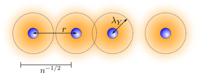
Figure 1: Edge-on schematic of a Yukawa monolayer. Charged particles (filled circles) are confined to a plane, while oppositely charged ions are free to move in the surrounding, unbounded 3D space. The mean ion density is color-coded. Typical in-plane nearest neighbor distances are similar to the mean geometric distance $n^{-1/2}$, and of the same order of magnitude as the Yukawa screening length $\lambda_{Y}$. Particle separations greatly exceed the particle diameter. The effective particle interactions are quantified by the two dimensionless parameters $\Gamma_{Y}$ and $\kappa_{Y}=1/(\lambda_{Y}\sqrt{n})$.

The Yukawa monolayer model implicitly assumes thermodynamic equilibrium statistics of ions, as schematically depicted in Fig. 1. Unlike the two-dimensionally confined, mesoscopic charged particles, ions are free to move in 3D space in the absence of external forces. Under these conditions the effective interaction potential $U_{Y}(x)$ between charged particles at sufficiently large mutual distance follows the screened Coulomb (Yukawa)-type form Khrapak et al. (2010)

$$\frac{U_{Y}(x)}{k_{\text{B}}T}=\Gamma_{Y}\dfrac{\exp(-\kappa_{Y}x)}{x},$$ (1)

where $k_{B}$ is Boltzmann’s constant, $T$ is the absolute temperature, and $x=r\sqrt{n}$ is the particle center-to-center distance in units of the mean geometric distance $n^{-1/2}$.

The Yukawa potential in Eq. (1) is characterized by the two dimensionless parameters $\Gamma_{Y}$ and $\kappa_{Y}$: The coupling parameter $\Gamma_{Y}=Q_{Y}^{2}\sqrt{n}/(4\pi\epsilon k_{\text{B}}T)$ quantifies the interaction strength in terms of the charged particle’s effective Yukawa charge $Q_{Y}$ (which is typically less than the bare electric charge of the particles Kennedy and Allen (2003); Morfill and Ivlev (2009)), and the dielectric permittivity $\epsilon$ of the embedding medium. In case of dusty plasmas, $\epsilon$ is equal to the dielectric permittivity of vacuum, $\epsilon_{0}$, for all purposes of the present article in which we adhere to SI units. The screening parameter, $\kappa_{Y}=1/(\lambda_{Y}\sqrt{n})$, is the normalized inverse of the Debye screening length $\lambda_{Y}$, which depends on the ion population. In an embedding plasma that consists of neutral particles and univalent positive ions only, $\lambda_{Y}=\sqrt{\epsilon k_{B}T/(e^{2}n_{i})}$ is the Debye length in terms of the proton elementary charge $e$, and the unperturbed (3D) ion number density $n_{i}$ of the ions far from the charged particle’s confining plane.

The Yukawa model in two dimensions is best realized experimentally for charged colloids which are confined between two highly charged glass plates Chang and Hone (1988); Löwen (1992); Barreira Fontecha et al. (2005). There, the screening is caused by the microions between the plates Chang and Hone (1988) and it can be tuned by adding salt. The experimentally observed freezing phase sequence has been found to agree with the theoretical predictions assuming a 2D Yukawa interaction Barreira Fontecha et al. (2005).

II.2 Kompaneets monolayer

The second class of systems studied in this article is schematically depicted in Fig. 2. A radio frequency discharge chamber contains a weakly ionized plasma (of neutral gas particles, electrons, and ions), and negatively charged dust particles are levitating atop an electrode on the bottom of the chamber. Confinement of the dust particles to a well-defined 2D layer is achieved by a force balance between gravitation and electrostatic repulsion. Unlike the particles in the spatially unbounded Yukawa system, the ions in the radio frequency chamber exhibit a highly non-equilibrium steady state with a non-zero plasma current towards the electrode, where positive ions are adsorbed. Attraction between dust particles and ions causes downstream focusing of ions in the so-called plasma wake region. As a consequence, every dust particle trails a positive space-charge in the downstream direction, which causes the effective pair-potential between charged dust particles to be anisotropic in 3D.

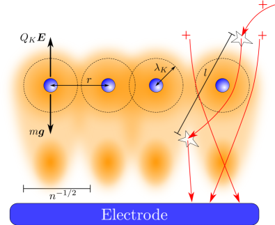
Figure 2: Edge-on schematic of a dusty plasma monolayer. Negatively charged dust particles (filled circles) levitate in a well-defined 2D layer above an electrode in a radio frequency discharge plasma chamber, at a height where gravity is balanced by the vertical electrostatic force. The mean distribution of ions is color-coded. Three characteristic ion trajectories are sketched by arrows signed with $+$. Subsequent collisions between ions and neutral particles are separated on average by the ion-neutral mean free path $l$. Ions are focused in the downstream direction below the dust particles, giving rise to positive space-charges in the plasma wake region. The effective dust particle interactions are quantified by the three dimensionless parameters $\Gamma_{K}$, $\kappa_{K}=1/(\lambda_{K}\sqrt{n})$, and $\zeta=\lambda_{K}/l$.

Kompaneets et al. Kompaneets et al. (2007) have presented a self-consistent steady-state solution for the effective pair potential between the dust particles, taking into account the external electric field E towards the electrode, and the collisions between ions and electrically neutral particles in the plasma. The resulting effective particle pair-potential, obtained under the assumptions of the mobility-limited ion drift in the field E, velocity-independent ion-neutral scattering cross section, and further assumptions that are outlined in the original reference, has been derived and described comprehensively in Ref. Kompaneets et al. (2007). We will refer to this kinetic pair-potential as the Kompaneets pair potential. For particles that are perfectly confined to a plane perpendicular to the plasma current, the in-plane Kompaneets potential $U_{K}(x)$ is given by

$$\begin{split}\frac{U_{K}(x)}{k_{\text{B}}T}=&~{}\Gamma_{K}~{}\dfrac{2\zeta\kappa_{K}}{\pi}~{}\text{Re}\int_{0}^{\infty}\frac{dt}{1+\zeta^{-2}Y(t)}\\ &\times K_{0}\left(x\zeta\kappa_{K}\sqrt{\frac{t^{2}+\zeta^{-2}X(t)}{1+\zeta^{-2}Y(t)}}\right),\end{split}$$ (2)

where $K_{0}$ is the zeroth-order modified Bessel function of the second kind Abramowitz and Stegun (1965), and the two auxiliary functions $X(t)$ and $Y(t)$ are defined as

$$\begin{split}&X(t)=1-\sqrt{1+it},\\ &Y(t)=\frac{2\sqrt{1+it}}{it}\int_{0}^{1}\frac{d\alpha}{[1+it(1-\alpha^{2})]^{2}}-\frac{1}{it(1+it)}.\end{split}$$ (3)

In Eq. (2), the prefactor $\Gamma_{K}=Q_{K}^{2}\sqrt{n}/(4\pi\epsilon k_{\text{B}}T)$ quantifies the interaction strength in terms of the effective charge $Q_{K}$, and the screening parameter is defined as $\kappa_{K}=1/(\lambda_{K}\sqrt{n})$, where $\lambda_{K}=\sqrt{\epsilon El/(e^{2}n_{i})}$ is a field-induced screening length. In addition, the Kompaneets potential depends on the collision parameter $\zeta=\lambda_{K}/l$, where $l$ is the mean free path between two consecutive collisions of an ion and neutral gas particles (“ion-neutral mean free path”, for short).

For close-contact configurations ($r\ll\zeta^{s}\lambda_{K}$, where $1/3\leq s\leq 1$, depending on the magnitude of $\zeta$ Kompaneets et al. (2007)), the Kompaneets potential tends to the bare Coulomb potential:

$$x\ll\zeta^{s}/\kappa_{K}:\qquad\frac{U_{K}(x)}{k_{\text{B}}T}\to\dfrac{\Gamma_{K}}{x}.$$ (4)

Hence, the Coulomb potential is recovered at all distances $x$ in the limit $\zeta\to\infty$, corresponding to a very large field $E$, or a very small ion mean free path $l$ or/and ion density $n_{i}$. For large particle separations and finite values of $\zeta$, the Kompaneets potential reduces to its in-plane asymptotic form

$$\left.\frac{U_{K}(x)}{k_{\text{B}}T}\right|_{x\to\infty}=\dfrac{\Gamma_{K}}{6\sqrt{2}\kappa_{K}^{2}x^{3}}\left(60\zeta^{2}-1\right)+\mathcal{O}(x^{-4}).$$ (5)

The leading order asymptotic form of the anisotropic out-of-plane electrostatic potential is proportional to $x^{-2}$, and is given in Eq. (8) of Ref. Kompaneets et al. (2007) (in Gaussian units).

In typical dusty plasma experiments the effective interaction potential can be measured for particle distances $x\approx 1$ (i.e., close to the mean geometric distance) by particle video tracking Konopka et al. (2000). It has been shown in Ref. Kompaneets et al. (2007), that the pair-potential in the experimentally directly accessible narrow range of particle separations can be fitted equally well by the Yukawa as well as the Kompaneets form. However, one should expect that the qualitative differences between the Yukawa and Kompaneets potentials, most particularly in their long-ranged asymptotic forms, can have a considerable influence on collective dynamics Röcker et al. (2012) and phase transitions.

III Mode Coupling Theory

The glassy state is characterized by liquid-like static pair correlations without long range order, and a non-zero value of the non-ergodicity parameter $f_{q}=\lim_{t\rightarrow\infty}\phi_{q}(t)$, which is the long time limit of the wavenumber- and time-dependent autocorrelation function $\phi_{q}(t)$ of the number density. The parameter $f_{q}$ is also called the form factor or the Debye-Waller factor. In contrast to the glassy state, the liquid state is characterized by a vanishing non-ergodicity parameter, $f_{q}=0$, for all wavenumbers $q$. In MCT, $f_{q}$ is calculated as Bengtzelius et al. (1984); Götze (2009)

$$\frac{f_{q}}{1-f_{q}}=\mathcal{F}_{q}[f],$$ (6)

where in 2D Bayer et al. (2007)

$$\mathcal{F}_{q}[f]=\frac{S_{q}}{8\pi^{2}q^{4}}\int d^{2}k~{}S_{k}S_{p}\left(\mathbf{q}\cdot\mathbf{k}~{}c_{k}+\mathbf{q}\cdot\mathbf{p}~{}c_{p}\right)^{2}f_{k}f_{p},$$ (7)

with $\mathbf{p}=\mathbf{q}-\mathbf{k}$.

The static structure factor $S_{q}$ and direct correlation function $c_{q}=1-1/S_{q}$ are the only input to the MCT equations, conveying information about the particle interactions. Note that the number density $n$ does not explicitly enter into Eq. (7), since all lengths and wave vectors are expressed in units of $1/\sqrt{n}$ and $\sqrt{n}$, respectively: In our notation the wave vector $\boldsymbol{q}$ is the dimensionless Fourier conjugate variable to the dimensionless distance vector $\boldsymbol{x}=\boldsymbol{r}\sqrt{n}$.

The Lamb-Mössbauer factor $f^{s}_{q}=\lim_{t\rightarrow\infty}\phi^{s}_{q}(t)$, which is the long-time limit of the wavenumber- and time-dependent, Fourier transformed tagged particle position autocorrelation function $\phi^{s}_{q}(t)$, is calculated in MCT according to Fuchs et al. (1998)

$$\frac{f^{s}_{q}}{1-f^{s}_{q}}=\mathcal{F}^{s}_{q}[f,f^{s}],$$ (8)

where Bayer et al. (2007)

$$\mathcal{F}^{s}_{q}[f,f^{s}]=\frac{1}{4\pi^{2}q^{4}}\int d^{2}k~{}S_{k}(\mathbf{q}\cdot\mathbf{k})^{2}c_{k}^{2}f_{k}f^{s}_{p}$$ (9)

and, once again, $\mathbf{p}=\mathbf{q}-\mathbf{k}$.

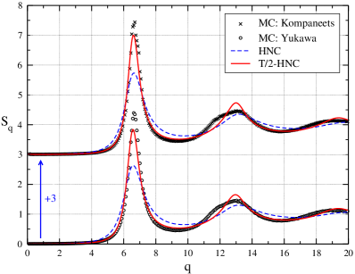
Figure 3: Static structure factors for a Yukawa monolayer with $\Gamma_{Y}=100$ and $\kappa_{Y}=2.0$ (lower three data sets) and a Kompaneets monolayer with $\Gamma_{K}=300$, $\kappa_{K}=2.0$, and $\zeta=0.25$ (upper three datasets). Crosses and circles: Monte Carlo simulation results. Dashed curves: HNC integral equation solution. Solid curves: Solution of the T/2-HNC in Eq. (10). The Kompaneets monolayer structure factors are shifted by $3$ units along the vertical axis for clarity.

We evaluate the integrals in Eqs. (7) and (9) numerically and solve Eqs. (6) and (8) iteratively with iteration seeds ${f_{q}}^{0}={f^{s}_{q}}^{0}=1$ Franosch et al. (1997). To evaluate the integrals numerically we use $N=200$ equidistant grid points with spacing $\Delta q=0.2$, minimal wavenumber $q_{\text{min}}=0.1$ and maximal wavenumber $q_{\text{max}}=39.9$. Test calculations with $N=500$ grid points allow us to estimate the numerical error due to integral discretization, which is around $5\%$ in the glass transition temperatures. The static structure factor is obtained from the (Fourier transformed) solution of the T/2-HNC integral equation Hajnal et al. (2011)

$$\gamma(x)=\int d^{2}x^{\prime}~{}c(|\mathbf{x}-\mathbf{x}^{\prime}|)\left[\exp\left\{\gamma(x^{\prime})-\dfrac{\displaystyle{2U(x^{\prime})}}{\displaystyle{k_{B}T}}\right\}-1\right],$$ (10)

for an isotropic 2D fluid in terms of the indirect and direct correlation functions $\gamma(x)$ and $c(x)$ Hansen and McDonald (1986). Equation (10) is solved by means of a numerical spectral solver for liquid integral equations in an arbitrary number of spatial dimensions, which has been comprehensively described in Ref. Heinen et al. (2014), and which is based on methods that have been originally introduced in Refs. Ng (1974); Talman (1978); Rossky and Friedman (1980); Hamilton (2000); Ham . The spectral solver operates on logarithmically spaced grids of wavenumbers and radii, providing a high-resolution structure factor that is mapped to the above mentioned equidistant wavenumber grid by quadratic interpolation.

Note that Eq. (10) is a simple modification of the well-known hypernetted chain (HNC) integral equation Morita (1958); Hansen and McDonald (1986), which is recovered when the term $2U(x^{\prime})$ in the integrand is replaced by $U(x^{\prime})$. Thus, the solution of the T/2-HNC equation coincides exactly with the solution of the HNC integral equation for a system in which the temperature has been scaled down by a factor of $1/2$. In Ref. Hajnal et al. (2011), the MCT glass transition was studied for two-dimensional binary mixtures of aligned point-dipoles with a long-ranged repulsive pair potential that is proportional to the inverse cube of the particle separation, $r^{-3}$. It was empirically found in Ref. Hajnal et al. (2011) that the T/2-HNC scheme predicts the static structure factors of the strongly repulsive 2D binary dipole mixtures with a significantly higher accuracy than the HNC scheme. In order to test the accuracy of the T/2-HNC scheme for the Yukawa- and Kompaneets monolayer systems, we have simulated 2D equilibrium liquids with strong repulsive pair potentials of both types, and compared the static structure factor from the simulation to the HNC and the T/2-HNC scheme solutions. Our results, shown in Fig. 3, underpin the good accuracy of the T/2-HNC and its supremacy over the HNC scheme. We have obtained the datasets represented by crosses and circles in Fig. 3 from Metropolis Monte Carlo (MC) simulations in the $NLT$-ensemble of constant particle number $N$, constant system area $L^{2}$, and constant temperature $T$. A square simulation box with periodic boundary conditions in both Cartesian directions was used in our simulations, and we haven chosen the parameters $\Gamma_{Y}=100$ and $\kappa_{Y}=2.0$ for the Yukawa monolayer of $N=10.000$ particles and $\Gamma_{K}=300$, $\kappa_{K}=2.0$, and $\zeta=0.25$ for the Kompaneets monolayer of $N=12.000$ particles. Both simulated systems are strongly coupled equilibrium liquids not far from the crystal-liquid transition point. In our MC simulations, the direct particle interactions are truncated at a dimensionless cutoff radius of $x_{c}=r_{c}\sqrt{n}=5$ in case of Yukawa interactions, and at $x_{c}=12.5$ in case of Kompaneets interactions. For pair separations $x>x_{c}$, the pair-potential is set equal to zero in the simulations. Varying its numerical value, we have checked that the cutoff radius is large enough and does not have a significant effect on the measured quantity $S_{q}$.

Note from Fig. 3 that despite its improved accuracy in comparison to the standard HNC scheme, the T/2-HNC scheme still tends to underestimate the principal peak height in $S_{q}$. In addition note that we apply the T/2-HNC scheme in the following sections to systems at the liquid-glass transition, that is, beyond the equilibrium fluid regime for which the accuracy of the integral equation scheme can be tested by comparison to crystallization-free simulations. Moreover, the approximate T/2-HNC scheme is combined in the following with the approximate MCT equations. The combined uncertainty of the resulting glass transition lines cannot be easily estimated and, thus, the numerical values of the glass transition temperatures must be taken with some caution. Nevertheless, the dominating qualitative features of $S_{q}$ are contained in the T/2-HNC solution, and the features of the glass transition curves can be expected to be at least qualitatively correct.

It is important to note also that the T/2-HNC scheme is empirically justified only in case of strong enough particle interactions. In the limit of vanishing interactions, $\Gamma_{Y}\to 0$ or $\Gamma_{K}\to 0$, the T/2-HNC scheme predicts twice the correct asymptote $c(r)\to\exp\left\{-U(r)/k_{B}T\right\}-1$ for the direct correlation function (i.e., twice the Mayer function). A related issue is the wrong long-distance decay – the T/2-HNC scheme yields twice the correct expression $\lim_{r\to\infty}c(r)=-U(r)/k_{B}T$. This wrong long-distance decay is observed for all values of the potential prefactor.

IV Results

IV.1 Glass transition diagrams

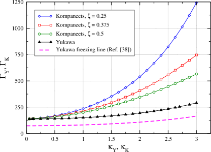
Figure 4: Glass transition curves in the ($\kappa,\Gamma$)-plane, for the Yukawa potential (black curve with triangles) and three different Kompaneets potentials with parameters $\zeta=0.25$ (solid curves with diamonds), $\zeta=0.375$ (solid curve with squares) and $\zeta=0.5$ (solid curve with circles). The dashed curve is the 2D Yukawa freezing line from Ref. Hartmann et al. (2005).

The glass transition curves for the Yukawa monolayer, and for three different Kompaneets-monolayers with different values of the collision parameter $\zeta$, are shown in the transition diagram in Fig. 4. In the transition diagram, the screening parameters $\kappa_{Y}$ and $\kappa_{K}$ vary along the horizontal axis, and the coupling parameters $\Gamma_{Y}$ and $\Gamma_{K}$ vary along the vertical axis. The data points in Fig. 4 represent the lowermost values of $\Gamma_{Y,K}$ for which $f_{q}$ assumes a non-zero value at given values of $\kappa_{Y,K}$. Note that at the glass transition, $f_{q}>0$ for all finite values of $q$ smaller than the $q$ cutoff. In our implementation, we have tested $f_{q}$ at $q=3.9$ to identify the glass transition points. In the One-Component-Plasma (OCP) limit $\kappa_{Y,K}\to 0$, both the Yukawa and the Kompaneets potential reduce to the unscreened Coulomb potential [see Eqs. (1) and (4)], and the glass transition curves close in on the T/2-HNC-MCT approximation for the OCP glass transition point, $\Gamma_{Y}=\Gamma_{K}=138.5$.

While the glass transition curves are qualitatively similar for the Yukawa and the Kompaneets systems, the transition occurs at higher values of the coupling parameter in case of the Kompaneets monolayer. For decreasing values of the parameter $\zeta$, the differences between the Yukawa and Kompaneets glass transition curves are increasing. Such trend is not surprising: As we discuss in the next subsection (see also Fig. 5), the deviation of the Kompaneets potential from the Yukawa-like form drastically increases as $\zeta$ decreases. On the other hand, in the limit $\zeta\to\infty$ the Kompaneets potential tends to the Coulomb form, so the Kompaneets glass transition curve in this case would be a horizontal line in the transition diagram of height $\Gamma_{K}=138.5$.

For 3D Yukawa systems it has been found that the glass transition and crystallization (freezing) lines are approximately parallel in the $(\kappa_{Y},\Gamma_{Y})$-plane Yazdi et al. (2014). The same similarity between the glass transition and crystallization lines is found for the 2D Yukawa monolayer in Fig. 4, where we plot the 2D Yukawa freezing line reproduced from Ref. Hartmann et al. (2005) (dashed curve), and the T/2-HNC-MCT 2D Yukawa glass transition line (black curve with triangles). In Ref. Hartmann et al. (2005), the crystallization line was obtained from simulations, and it was approximated by the inverse polynomial $\Gamma=\Gamma^{\ast}/(1+f_{2}\kappa^{2}+f_{3}\kappa^{3}+f_{4}\kappa^{4}$), with $\Gamma^{\ast}=73.9=131/\sqrt{\pi}$, $f_{2}=-0.1235$, $f_{3}=0.0248$ and $f_{4}=-0.0014$. Note that the 2D ion-sphere radius $a=1/\sqrt{\pi n}$ (also called Wigner-Seitz radius) was used as a unit of length in Ref Hartmann et al. (2005), instead of the mean geometric distance $1/\sqrt{n}$ utilized in the present paper. Therefore, one has to take account of a $1/\sqrt{\pi}$ prefactor difference in the definitions of the Yukawa coupling parameter and the inverse Yukawa screening parameter.

IV.2 Potentials and structure factors at the glass transition

In Fig. 5 we plot the Yukawa potential and three different in-plane Kompaneets potentials for different values of $\zeta$, all at the glass transition for $\kappa_{Y}=\kappa_{K}=2.0$. The full set of parameters, including the glass transition values of $\Gamma_{Y}$ and $\Gamma_{K}$, is provided in the figure caption. Note that the potentials in Fig. 5 are multiplied by their argument $x=r\sqrt{n}$, to expose the differences. The curves corresponding to Kompaneets pair-potentials (with $r^{-3}$ asymptotics) therefore decay proportionally to $x^{-2}$ for large values of $x$. The inset of Fig. 5 features the T/2-HNC static structure factors $S_{q}$, corresponding to the four different potentials plotted in the figure’s main panel. Despite the pronounced differences between the four potentials (in particular around the most frequently sampled mean geometric distance $x=1$), all four functions $S_{q}$ at the glass transition are indistinguishable on the scale of the figure inset. The principal peak heights of the four structure factors differ only slightly in their values.

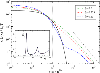
Figure 5: Effective pair-potentials for $\kappa_{Y}=\kappa_{K}=2.0$, for values of $\Gamma_{Y}$ and $\Gamma_{K}$ at the liquid-glass transition point. Solid curve: Yukawa potential for $\Gamma_{Y}=195.4$. Dashed, dot-dashed and dot-dot-dashed curves: Kompaneets potentials for $\zeta=0.25,0.375$ and $0.5$, and $\Gamma_{K}=539.4,406.8$ and $345.0$, respectively. All potentials are multiplied by their argument, $x=r\sqrt{n}$, to expose the differences. The inset features the corresponding static structure factors $S_{q}$ in T/2-HNC approximation. All four functions $S_{q}$ are overlapping on the scale of the inset. The principal peak heights of the structure factors are $S_{q}=6.33$ for the Yukawa system, and $S_{q}=6.26,6.23$ and $6.19$ for the Kompaneets systems with $\zeta=0.5,0.375$ and $0.25$, respectively.

IV.3 A fallacious re-entrant state sequence

As pointed out in Sec. II, the 2D Yukawa model with its many simplifying assumptions is merely a toy model for experimentally observable monolayers of mesoscopic charged particles. For the important class of ground-based dusty plasma experiments the kinetic pair-potentials are far more realistic, and among them the Kompaneets pair potential stands out with its realistic model assumptions. In this section, we allude to the possible consequences of an over-simplified interpretation of charged particle monolayers in terms of the Yukawa model. We show that the liquid-glass transition of a system with Kompaneets-like pair potential appears as a non-monotonic curve (corresponding to liquid-glass-liquid state re-entrance) when it is plotted in terms of the inappropriate parameters of the Yukawa potentials that represent a best fit to the actual (Kompaneets) potential around the mean geometric distance $x=r\sqrt{n}=1$.

In Fig. 6 we plot the Yukawa glass transition curve that is also shown in Fig. 4 (black curves with triangles). The 2D Yukawa freezing line, reproduced from Ref. Hartmann et al. (2005), is also shown (dashed line) to allow a better comparison to the glass transition line than on the scale of Fig. 4. The curve with open squares in Fig. 6 is generated as follows: For given values of the two Yukawa parameters $\kappa_{Y}$ and $\Gamma_{Y}$, we calculate the Kompaneets potential that fits best to the Yukawa potential in the distance range $0.7<x<3$ which is most frequently sampled by the particles Konopka et al. (2000). The fit is conducted as follows: For given values of $l$ and $n$, which yields the combination $\zeta\kappa_{K}\equiv(l\sqrt{n})^{-1}$ ($\simeq 0.354$ for the example shown in the figure), we tune the two remaining, independent Kompaneets parameters $\kappa_{K}$ and $\Gamma_{K}$; an optimal fit is achieved by minimizing the square deviation $\int_{0.7}^{3}dx{[U_{Y}(x)-U_{K}(x)]}^{2}$ between the two potentials. We then calculate $S_{q}$ for the best-fitting Kompaneets potential in the T/2-HNC scheme, and use it as the input to the MCT equations (6) and (7) for $f_{q}$. If $f_{q}=0$, the system is classified as liquid, and if $f_{q}>0$, it is classified to be in the glassy state. We repeat the full procedure for various Yukawa parameters $\kappa_{Y}$ and $\Gamma_{Y}$, which are tuned by interval bisection, until we find for each $\kappa_{Y}$ the smallest (critical) value of $\Gamma_{Y}$ at which the best-fitting Kompaneets system vitrifies.

Thus, the curve with open squares in Fig. 6 is the glass transition curve of a dusty plasma monolayer with Kompaneets-like interactions, as it would appear when plotted in terms of the dimensionless parameters $\kappa_{Y}$ and $\Gamma_{Y}$ of the Yukawa potentials that best fit the actual Kompaneets potential around the mean geometric distance, where the potential is directly accessible Konopka et al. (2000). Therefore, if one observes vitrification in a dusty plasma monolayer and assumes Yukawa-like interactions in the experiment analysis, the transition behavior may be misinterpreted as a re-entrant liquid-glass-liquid state sequence, while the transition diagram in terms of the three relevant Kompaneets potential parameters does not exhibit any re-entrance (see Fig. 4).

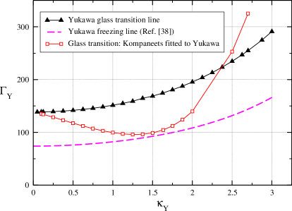
Figure 6: Kompaneets and Yukawa glass transitions in the Yukawa parameter plane. The curve with triangles: Yukawa glass transition curve in the Yukawa screening- and coupling-parameter ($\kappa_{Y},\Gamma_{Y}$)-plane. The curve with squares is the glass transition curve for Kompaneets pair-potentials which have been optimally fitted to the corresponding Yukawa potential in the region $0.7<x<3$, by pointwise tuning of the Kompaneets screening parameter $\kappa_{K}$ and coupling parameter $\Gamma_{K}$. The parameters $l=2.3$ mm and $n=1.5$ mm^-2 are held fixed for the Kompaneets potential. The dashed curve is the 2D Yukawa freezing line from Ref. Hartmann et al. (2005).

IV.4 Non-ergodicity parameters

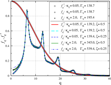
Figure 7: The Lamb-Mössbauer factors $f^{s}_{q}$ (monotonically decaying as functions of $q$) and the form factors $f_{q}$ (non-monotonic functions of $q$) for various Yukawa monolayers (symbols) and Kompaneets monolayers (curves) at their respective MCT glass transition points, with potential parameters as indicated in the legend.

We turn our attention now to the $q$-dependent Debye-Waller and Lamb-Mössbauer factors at the glass transition, which are plotted in Fig. 7. It is observed that $f_{q}$ approaches zero in the limit $q\to\infty$. In the opposite limit $q\to 0$, the functions $f_{q}$ for Yukawa- and Kompaneets potentials with a small value of the screening parameter $\kappa_{Y}=\kappa_{K}=0.05$ assume very small but non-zero values, and for finite wavenumbers $q$, all plotted functions $f_{q}$ deviate clearly from zero. Finite wavelength density modulations, cannot relax in the glassy state since this would require a collective rearrangement of particles on the length scale of some nearest neighbor cage diameters. Observing Fig. 7 and the inset of Fig. 5, one can see that the most resilient density modulations (corresponding to the principal maximum in $f_{q}$) are for $q\approx 2\pi$, that is, at the wavenumber that corresponds to the static structure factor principal maximum, and to the Fourier conjugate of the nearest neighbor (mean geometric) distance. Very long wavelength ($q\to 0$) density modulations cannot relax in the glassy state in general, as indicated by the finite values of $f_{q\to 0}$ in Fig. 7. This is due to the finite isothermal compressibility, $S_{q\to 0}$, of the system. Note here in particular that the Debye-Waller factor of hard-sphere system remains finite as $q$ approaches zero Franosch et al. (1997), which is in line with the rather large compressibility of such hard-sphere system. However, in the OCP limits $\kappa_{Y}\to 0$ and $\kappa_{K}\to 0$, in which both the Yukawa and the Kompaneets potential reduce to the Coulomb potential, the isothermal osmotic compressibility coefficient vanishes Baus and Hansen (1980); Hansen and McDonald (1986), which corresponds to an infinite thermodynamic driving force for the leveling of long-wavelength density modulations. Therefore, $f_{q\to 0}=0$ in the OCP limit.

The Yukawa- and Kompaneets system are indistinguishable in the OCP limit. This facilitates computation of the OCP-limiting behavior in terms of a small-q asymptotic expansion of the Yukawa monolayer Debye-Waller factor. As demonstrated in the Appendix, the T/2-HNC solution for the direct correlation function of a Yukawa monolayer can be approximated as

$$c_{q}\approx-\dfrac{2U_{Y}(q)}{k_{B}T}=-\dfrac{4\pi\Gamma_{Y}}{\sqrt{\kappa_{Y}^{2}+q^{2}}}~{}~{}~{}\text{for}~{}q+q_{t}\gg\kappa_{Y}^{2}+q^{2},$$ (11)

that is, when both the wavenumber $q$ and the screening parameter $\kappa_{Y}$ are small and within a certain ratio of each other. In Eq. (11), $q_{t}$ is a dimensionless non-negative threshold wavenumber with a typical value of $q_{t}\sim 0.1$. The corresponding small-$q$, small-$\kappa_{Y}$ form of $\mathcal{F}_{q}$ is obtained from a functional Taylor expansion Bayer et al. (2007); Yazdi et al. (2014), resulting in

$$\mathcal{F}_{q}=(\alpha+\beta q^{2}\ldots)S_{q}$$ (12)

where $S_{q}=(1-c_{q})^{-1}$,

$$\alpha=\frac{1}{4\pi}\int~{}dk~{}kS_{k}^{2}\left(c_{k}^{2}+kc_{k}c_{k}^{\prime}+\frac{3}{8}k^{2}{c^{\prime}}_{k}^{2}\right)f_{k}^{2}$$ (13)

and

$$\begin{split}\beta=&\frac{1}{8\pi}\int~{}dk~{}kS_{k}^{2}\left({c^{\prime}_{k}}^{2}+\frac{5}{32}k^{2}{c^{\prime\prime}_{k}}^{2}+\frac{3}{2}kc^{\prime}_{k}c^{\prime\prime}_{k}\right.\\ &\left.+c_{k}c^{\prime\prime}_{k}+\frac{1}{4}kc_{k}c^{\prime\prime\prime}_{k}+\frac{5}{24}k^{2}c^{\prime}_{k}c^{\prime\prime\prime}_{k}\right)f_{k}^{2}.\end{split}$$ (14)

Considering only the leading order of the approximation, this translates into the small-$q$, small-$\kappa_{Y}$ limiting behavior of the Yukawa monolayer Debye-Waller factor,

$$f_{q}={\alpha\left[1+\alpha+\dfrac{4\pi\Gamma_{Y}}{\sqrt{\kappa_{Y}^{2}+q^{2}}}\right]}^{-1}~{}~{}~{}\text{for}~{}q+q_{t}\gg\kappa_{Y}^{2}+q^{2},$$ (15)

in T/2-HNC approximation. For finite $\kappa_{Y}$, the function $f_{q}$ in Eq. (15) assumes a positive value for $q=0$, and increases $\propto q^{2}$ when $q\to 0$. Only in the OCP limit $\kappa_{Y}=0$, the function $f_{q}$ in Eq. (15) vanishes for $q=0$, and increases initially as $\propto q$. In a broad scale the $f_{q}$ asymptotic for $\kappa_{Y}=0.05$ and $\Gamma_{Y}=138.7$ is almost linear.

Note here that the small-$q$ limiting OCP Debye-Waller factor is qualitatively different in two and three dimensions. In 3D, the function $f_{q}$ vanishes in the OCP limit $\kappa_{Y}=0$ as $\propto q^{2}$ Yazdi et al. (2014). In contrast to $f_{q}$, the Lamb-Mössbauer factor $f^{s}_{q}$ in MCT approximation does not critically depend on the form of the pair potential, since $\mathcal{F}^{s}_{q}$ in Eq. (9) and also the small-$q$ limit of $\mathcal{F}^{s}_{q}$ Bayer et al. (2007) do not depend on $S_{q}$.

V Conclusions

We have calculated the liquid-glass transition boundaries in the state diagram spanned by the screening parameters and coupling parameters of 2D monolayers with Yukawa- and Kompaneets-like pair potentials, in T/2-HNC-MCT approximation. While both types of systems exhibit qualitatively similar glass transition curves, there is a quantitative difference in the vitrification temperature, which decreases as a function of the collision parameter $\zeta$ of the Kompaneets pair-potential. Both the Kompaneets- and Yukawa-monolayer reduce to a two-dimensionally confined OCP in the limit of infinite $\lambda_{Y}$ and $\lambda_{K}$.

In contrast to the over-simplifying 2D Yukawa model, the kinetic pair-potentials, including in particular the Kompaneets pair-potential, provide far more accurate descriptions of the interactions between dust grains in typical ground-based complex plasma experiments. We have demonstrated that a glass transition in a dusty plasma monolayer is prone to a qualitative misinterpretation if the simple Yukawa model is invoked in its analysis: While the glass transition line is a monotonic function in terms of the three relevant, dimensionless Kompaneets pair-potential parameters, it appears to be non-monotonic corresponding to a fallacious liquid-glass-liquid re-entrance when the pair interactions are misinterpreted as Yukawa-type interactions.

A promising task for future research would be the generalization of our results to binary systems, in order to understand the different glass types in mixtures. Since the crystalline states in such systems are pretty complex Assoud et al. (2008), the glass transition scenarios are also expected to be much more complex than in the monodisperse system.

Appendix

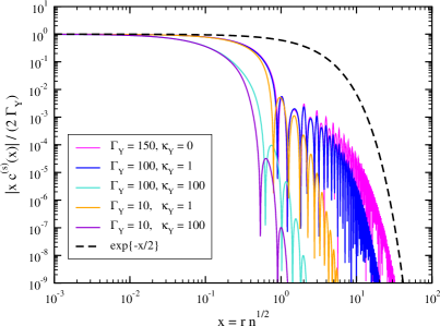
Figure 8: Function $|xc^{(s)}(x)|$ for Yukawa monolayers and various potential parameters, calculated in T/2-HNC approximation, is bound from above by $2\Gamma_{Y}\exp\left\{-x/2\right\}$.

Here we validate the small-$q$, small-$\kappa_{Y}$ result for the T/2-HNC direct correlation function of a Yukawa monolayer in Eq. (11). We begin by noting that the function $c(x)$ can be split into the sum

$$c(x)=c^{(s)}(x)-2\Gamma_{Y}\dfrac{\exp(-\kappa_{Y}x)}{x},$$ (16)

of a short-ranged part, $c^{(s)}(x)$, and the asymptotic long-ranged part, $-2\Gamma_{Y}\exp(-\kappa_{Y}x)/x$. In Eq. (16), the peculiar long-ranged asymptotics $c(x\to\infty)=-2U(x)/{k_{B}T}$ of the T/2-HNC scheme solution has been taken into account (c.f., our discussion at the end of Sec. III). The direct correlation function in wavenumber-space is calculated as the isotropic 2D Fourier transform (Hankel transform)

$$c_{q} =2\pi\int\limits_{0}^{\infty}~{}dx~{}xc(x)J_{0}(qx)$$

$$=\underbrace{2\pi\int\limits_{0}^{\infty}~{}dx~{}xc^{(s)}(x)J_{0}(qx)}_{\displaystyle{c_{1}}}-\underbrace{4\pi\int\limits_{0}^{\infty}~{}dx~{}e^{-\kappa_{Y}x}J_{0}(qx)}_{\displaystyle{c_{2}}},$$

where $J_{0}$ denotes the Bessel function of the first kind with index $0$. Note from Fig. 8 that the T/2-HNC scheme solution for the function $|xc^{(s)}(x)|$ is bound from above by the function $2\Gamma_{Y}\exp\{-x/2\}$ for all reasonable combinations of $\Gamma_{Y}$ and $\kappa_{Y}$, and even in the OCP limit $\kappa_{Y}=0$. This finding, combined with the upper bound $|J_{0}(x)|<\min\{1,\sqrt{2/(\pi x)}\}$ for the envelope of the Bessel function, allows us to compute an upper bound

$$|c_{1}|<\min\left\{12\pi\Gamma_{y},\dfrac{8\pi\Gamma_{Y}}{\sqrt{q}}\right\}.$$ (18)

for the modulus of the function $c_{1}(q)$. Solutions for all Hankel transforms occurring in such computation are listed in Ref. Erdélyi (1954). Noting that $c_{2}=4\pi\Gamma_{Y}/\sqrt{\kappa_{Y}^{2}+q^{2}}$, we conclude that $c_{1}$ in Eq. (Appendix) is negligible if the condition

$$q+q_{t}\gg\kappa_{Y}^{2}+q^{2}$$ (19)

is fulfilled, where $q_{t}\sim 0.1$ is a threshold wavenumber. For all combinations of $q$ and $\kappa_{Y}$ that fulfill Eq. (19), the T/2-HNC solution for $c_{q}$ is well approximated by $c_{q}\approx-c_{2}=4\pi\Gamma_{Y}/\sqrt{\kappa_{Y}^{2}+q^{2}}$.

References

- Ivlev et al. (2012) A. Ivlev, H. Löwen, G. Morfill, and C. P. Royall, Complex Plasmas and Colloidal Dispersions: Particle-Resolved Studies of Classical Liquids and Solids (World Scientific, Singapore, 2012).
- Pieranski et al. (1983) P. Pieranski, L. Strzelecki, and B. Pansu, Phys. Rev. Lett. 50, 900 (1983).
- Chang and Hone (1988) E. Chang and D. W. Hone, Europhys. Lett. 5, 635 (1988).
- Thomas et al. (1994) H. Thomas, G. E. Morfill, V. Demmel, J. Goree, B. Feuerbacher, and D. Möhlmann, Phys. Rev. Lett. 73, 652 (1994).
- Fortov et al. (2005) V. E. Fortov, A. V. Ivlev, S. A. Khrapak, A. G. Khrapak, and G. E. Morfill, Phys. Rep. 421, 1 (2005).
- Fortov and Morfill (2010) V. E. Fortov and G. E. Morfill, eds., Complex and dusty plasmas: from laboratory to space (CRC Press, Boca Raton, 2010).
- Konopka et al. (2000) U. Konopka, G. E. Morfill, and L. Ratke, Phys. Rev. Lett. 84, 891 (2000).
- Kompaneets et al. (2007) R. Kompaneets, U. Konopka, A. V. Ivlev, V. Tsytovich, and G. Morfill, Phys. Plasmas 14, 052108 (2007).
- Vladimirov and Nambu (1995) S. V. Vladimirov and M. Nambu, Phys. Rev. E 52, R2172 (1995).
- Vladimirov and Ishihara (1996) S. V. Vladimirov and O. Ishihara, Phys. Plasmas 3, 444 (1996).
- Ishihara and Vladimirov (1997) O. Ishihara and S. V. Vladimirov, Phys. Plasmas 4, 69 (1997).
- Xie et al. (1999) B. S. Xie, K. F. He, and Z. Q. Huang, Phys. Lett. A 253, 83 (1999).
- Lemons et al. (2000) D. S. Lemons, M. S. Murillo, W. Daughton, and D. Winske, Phys. Plasmas 7, 2306 (2000).
- Lapenta (2000) G. Lapenta, Phys. Rev. E 62, 1175 (2000).
- Schweigert (2001) V. A. Schweigert, Plasma Phys. Rep. 27, 997 (2001).
- Kompaneets et al. (2008) R. Kompaneets, S. V. Vladimirov, A. V. Ivlev, and G. E. Morfill, New J. Phys. 10, 063018 (2008).
- Röcker et al. (2012) T. B. Röcker, A. V. Ivlev, R. Kompaneets, and G. E. Morfill, Phys. Plasmas 19, 033708 (2012).
- Khrapak et al. (2010) S. A. Khrapak, A. V. Ivlev, and G. E. Morfill, Phys. Plasmas 17, 042107 (2010).
- Kennedy and Allen (2003) R. V. Kennedy and J. E. Allen, J. Plasma Phys. 69, 485 (2003).
- Morfill and Ivlev (2009) G. E. Morfill and A. V. Ivlev, Rev. Mod. Phys. 81, 1353 (2009).
- Löwen (1992) H. Löwen, J. Phys.: Condensed Matter 4, 10105 (1992).
- Barreira Fontecha et al. (2005) A. Barreira Fontecha, H. J. Schöpe, H. König, T. Palberg, R. Messina, and H. Löwen, J. Phys.: Condens. Matter 17, S2779 (2005).
- Abramowitz and Stegun (1965) L. Abramowitz and I. A. Stegun, Handbook of mathematical functions with formulas, graphs, and mathematical tables (Dover Publications, Inc., New York, 1965), 9th ed., ISBN 0-486-61272-4.
- Bengtzelius et al. (1984) U. Bengtzelius, W. Götze, and A. Sjölander, J. Phys. C 17, 5915 (1984).
- Götze (2009) W. Götze, Complex Dynamics of Glass-Forming Liquids: A Mode-Coupling Theory (Oxford University Press, Oxford, 2009).
- Bayer et al. (2007) M. Bayer, J. Brader, F. Ebert, E. Lange, M. Fuchs, G. Maret, R. Schilling, M. Sperl, and J. P. Wittmer, Phys. Rev. E 76, 011508 (2007).
- Fuchs et al. (1998) M. Fuchs, W. Götze, and M. R. Mayr, Phys. Rev. E 58, 3384 (1998).
- Franosch et al. (1997) T. Franosch, M. Fuchs, W. Götze, M. R. Mayr, and A. P. Singh, Phys. Rev. E 55, 7153 (1997).
- Hajnal et al. (2011) D. Hajnal, M. Oettel, and R. Schilling, J. Non-Cryst. Solids 357, 302 (2011).
- Hansen and McDonald (1986) J.-P. Hansen and I. R. McDonald, Theory of Simple Liquids (Academic Press, London, 1986), 3rd ed.
- Heinen et al. (2014) M. Heinen, E. Allahyarov, and H. Löwen, J. Comput. Chem. 35, 275 (2014).
- Ng (1974) K.-C. Ng, J. Chem. Phys. 61, 2680 (1974).
- Talman (1978) J. D. Talman, J. Comput. Phys. 29, 35 (1978).
- Rossky and Friedman (1980) P. J. Rossky and H. L. Friedman, J. Chem. Phys. 72, 5694 (1980).
- Hamilton (2000) A. J. S. Hamilton, Mon. Not. R. Astron. Soc. 312, 257 (2000).
- (36) A. J. S. Hamilton’s FFTLog website, http://casa.colorado.edu/~ajsh/FFTLog/.
- Morita (1958) T. Morita, Prog. Theo. Phys. 20, 920 (1958).
- Hartmann et al. (2005) P. Hartmann, G. J. Kalman, Z. Donkó, and K. Kutasi, Phys. Rev. E 72, 026409 (2005).
- Yazdi et al. (2014) A. Yazdi, A. Ivlev, S. Khrapak, H. Thomas, G. E. Morfill, H. Löwen, A. Wysocki, and M. Sperl, Phys. Rev. E 89, 063105 (2014).
- Baus and Hansen (1980) M. Baus and J.-P. Hansen, Phys. Rep. 59, 1 (1980).
- Assoud et al. (2008) L. Assoud, R. Messina, and H. Löwen, J. Chem. Phys. 129, 164511 (2008).
- Erdélyi (1954) A. Erdélyi, ed., Tables of integral transforms. Based, in part, on notes left by Harry Bateman Volume II (McGraw-Hill, New York, 1954).