A radio-polarisation and rotation measure study of the Gum Nebula and its environment

Abstract

The Gum Nebula is $36\mbox{${}^{\circ}$}$-wide shell-like emission nebula at a distance of only $\sim 450$ pc. It has been hypothesised to be an old supernova remnant, fossil H II region, wind-blown bubble, or combination of multiple objects. Here we investigate the magneto-ionic properties of the nebula using data from recent surveys: radio-continuum data from the NRAO VLA and S-band Parkes All Sky Surveys, and H $\alpha$ data from the Southern H-Alpha Sky Survey Atlas. We model the upper part of the nebula as a spherical shell of ionised gas expanding into the ambient medium. We perform a maximum-likelihood Markov chain Monte-Carlo fit to the NVSS rotation measure data, using the H $\alpha$ data to constrain average electron density in the shell $n_{e}$. Assuming a latitudinal background gradient in RM we find $n_{e}=1.3^{+0.4}_{-0.4}\,\mbox{cm${}^{-3}$}$, angular radius $\phi_{\rm outer}=22.7^{+0.1}_{-0.1}\,{\rm degrees}$, shell thickness $dr=18.5^{+1.5}_{-1.4}\,{\rm pc}$, ambient magnetic field strength $B_{0}=3.9^{+4.9}_{-2.2}\,\mbox{$\mu$G}$ and warm gas filling factor $f=0.3^{+0.3}_{-0.1}$. We constrain the local, small-scale ($\sim 260$ pc) pitch-angle of the ordered Galactic magnetic field to $+7\mbox{${}^{\circ}$}\lesssim\wp\lesssim+44\mbox{${}^{\circ}$}$, which represents a significant deviation from the median field orientation on kiloparsec scales ($\sim-7.2\mbox{${}^{\circ}$}$). The moderate compression factor $X=6.0\,^{+5.1}_{-2.5}$ at the edge of the H $\alpha$ shell implies that the ‘old supernova remnant’ origin is unlikely. Our results support a model of the nebula as a H II region around a wind-blown bubble. Analysis of depolarisation in 2.3 GHz S-PASS data is consistent with this hypothesis and our best-fitting values agree well with previous studies of interstellar bubbles.

1 Introduction

Observations of atomic H I, molecular clouds and photo-dissociation regions in the Galaxy have shown that gas in a wide range of environments is gathered into spheres, bubbles or shell-like structures (e.g., Jackson et al. 2006; Churchwell et al. 2006; McClure-Griffiths et al. 2009). Most of these objects are formed by physical processes associated with the evolution of high-mass stars ($>8\,\mbox{M${}_{\odot}$}$). During their time on the main-sequence, such stars emit high fluxes of ultra-violet photons and fast winds of particles that ionise expanding H II regions, evacuate low-density cavities and sweep gas into shells in a ‘snow-plough’ effect. At the end of their lives the stars eject their outer layers, before exploding as supernovae, driving strong shocks into the interstellar medium (ISM). OB-type stars generally form in clusters, so the combined action of stellar winds and coeval supernova explosions can give rise to ‘supershells’, hundreds of parsecs in size (e.g., Moss et al. 2012). Supernovae and supershells are thought to power the circulation of material into the Galactic halo (Dove et al. 2000; Reynolds et al. 2001, Pidopryhora et al. 2007) and play a leading role in sculpting the fractal structure of gas in the Galactic disk. With energies greater than $\sim 10^{51}$ ergs, supernovae are also believed to be the main driver of turbulence in the disk (McCray & Snow 1979) and have been shown to trigger new episodes of star-formation when shocks overrun and compress pre-existing clumps of molecular gas (Reipurth 1983; Oey et al. 2005).

Spheres or bubbles of plasma also present an excellent opportunity to probe conditions in the ISM. Studies of individual objects can yield information on the conditions in the medium into which they are expanding and on their progenitors. Of particular interest are recent works that have used observations of Faraday rotation to derive the magneto-ionic properties of bubbles and their local ISM (e.g. Kothes & Brown 2009; Whiting et al. 2009; Harvey-Smith et al. 2011; Savage et al. 2013). As the bubbles expand they interact with the ordered magnetic field of the Galaxy, compressing the ambient medium and the field parallel to the shock front. The resulting field geometry is a function of the pre-existing field configuration and the rate of expansion, leading to a unique rotation measure (RM) signature on the sky. While observations of RMs from extra-galactic point sources yield only the average line-of-sight field strength, modelling the RM-signature of a supernova remnant or H II region is one of the few ways to measure the local magnetic field on scales of a few hundred parsecs. Such measurements are essential anchor-points for studies of the large-scale Galactic field (e.g., Kothes & Brown 2009).

If the line-of-sight magnetic field strength is known, Faraday rotation is a good tool to measure density jumps in the ionised ISM as $n_{e}\propto{\rm RM}$. The density jump present at the shell boundary is a key indicator of the type of object powering the expansion. For example, mass and momentum conservation in the radiatively cooling shock-fronts of old supernova remnants (SNR) are expected to lead to very high density jumps at their boundaries (Shull & Draine 1987). In contrast, the ionisation front of an evolved H II region created by a cluster of B-type stars would expand at the local sound speed (typically $\sim 10$ km s^-1), creating only a slight density jump. The level of compression and magnetic field strength in the ionised gas have profound implications for whether star formation is triggered or suppressed by the passing shock.

In this paper we present a study of one of the most prominent bubbles in the southern sky: the Gum Nebula. We start in $\S\ref{sec:gum_history}$ by reviewing the literature on the nebula, summarising its properties and theories of origin. In $\S\ref{sec:datasets}$ we introduce the datasets and images used in this work. We go on to describe our ionised shell model and analysis techniques in $\S\ref{sec:analysis}$. We present the results of fitting the model to the rotation measure data in $\S\ref{sec:results}$, where we derive strength and direction of the magnetic field, and the density jump across the edge of the nebula. Discussion and further analysis of depolarisation at radio wavelengths are presented in $\S\ref{sec:discussion}$. Finally, we present our conclusions in $\S\ref{sec:summary}$ and suggest future avenues of investigation.

1.1 The Gum Nebula

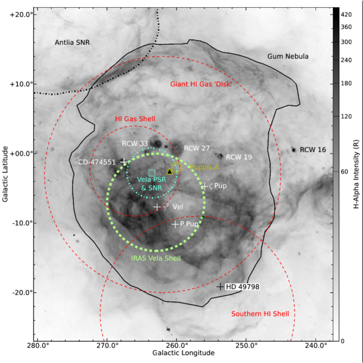
Figure 1: An H $\alpha$ image of the Gum Nebula (Finkbeiner 2003) annotated with significant objects identified in the literature. OB-type stars are marked with ‘+’ symbols, the Vela pulsar with a square and the kinematic centre of the nebula derived by Woermann et al. (2001) with a triangle. Boundaries of gas-disks or shells are marked using coloured circles. See $\S\ref{sec:gum_history}$ for details. References for the annotated objects are as follows: Antlia SNR: McCullough et al. 2002; Giant H I Gas Disk: Reynoso & Dubner 1997; H I Gas Shell: Dubner et al. 1992; IRAS Vela Shell: Sahu & Sahu 1993; RCW-H II regions: Rodgers et al. 1960; Vela Pulsar: Radhakrishnan & Manchester 1969; CD-474551: Reed 2003; HD 49798 and $\zeta$ Puppis: van Leeuwen 2007; $\gamma^{2}$ Velorum: De Marco & Schmutz 1999.

The Gum Nebula is one of the largest optical emission nebulae in the southern sky (Gum 1952). It has an approximately circular morphology with an angular diameter of $\sim 36\mbox{${}^{\circ}$}$ (Chanot & Sivan 1983), its centre is thought to lie at a distance of $\sim$500 pc from the Sun and its radius is $\sim 130$ pc (Woermann et al. 2001). Originally discovered in large-area photographic plates by Gum (1952), it dominates modern H $\alpha$ maps of the southern Galactic plane (e.g., Dennison et al. 1998; Gaustad et al. 2001; Haffner et al. 2003).

1.1.1 The environment of the Gum Nebula

Considerable controversy exists in the literature on the origin and evolution of the Gum Nebula. In part, this is because the nebula straddles the mid-plane of the Galaxy and its footprint encompasses a large number of overlapping objects: H II regions, supernova remnants (SNRs), OB-associations and molecular clouds. Early investigations of the nebula (e.g., Gum 1956; Brandt et al. 1971; Alexander et al. 1971; Beuermann 1973; Reynolds 1976b; Weaver et al. 1977; Vallee & Bignell 1983) were limited by the paucity of observations covering the entire region; however, more recent work has begun to form a clear picture (e.g., Sahu & Sahu 1992; Sahu & Sahu 1993; Duncan et al. 1996; Reynoso & Dubner 1997; Woermann et al. 2001; Stil & Taylor 2007). Fig. 1 presents an annotated H $\alpha$ image of the nebula in Galactic coordinates (Finkbeiner 2003) illustrating the principal structures identified to-date. The upper third of the nebula is relatively free of confusing sources except at $(l,b)\approx(268\mbox{${}^{\circ}$},+13\mbox{${}^{\circ}$})$ where the H $\alpha$ shell overlaps the Antlia supernova remnant (SNR, McCullough et al. 2002; Iacobelli et al. 2014). The lower two-thirds contain the majority of confusing objects, only some of which are directly associated with the Gum Nebula.

The energy budget of the nebula is dominated by the output of early-type stars: $\zeta$ Puppis; an O4f star, and $\gamma^{2}$ Velorum; a Wolf-Rayet star of type WC 8 with an O7.5 I companion (De Marco & Schmutz 1999). $\gamma^{2}$ Velorum is embedded in the Vela OB2 association, which contains a further 81 B-type stars at a mean distance of $415\pm 10$ pc (de Zeeuw et al. 1999). The combined flux from $\zeta$ Pup and $\gamma^{2}$ Vel is capable of maintaining the ionisation state of the Gum Nebula (Weaver et al. 1977), however, Vela OB2 also appears to be creating a smaller bubble within the Gum Nebula - the IRAS Vela Shell (IVS). The IVS was identified by Sahu & Sahu (1993) as a radius $=7.5\mbox{${}^{\circ}$}$ ring-like structure in the 100 $\mu$m IRAS Sky Survey Atlas centred on Vela OB2. It is associated with a thick shell of H I (Dubner et al. 1992) and swept-up molecular gas (Churchwell et al. 1996), and has been interpreted as a wind-blown bubble driven by Vela OB2 (Sahu & Sahu 1993). Two further OB-stars are in the field: the O6 star CD-47 4551 lies well beyond the Gum Nebula at a distance of $\sim 1300$ pc, too far to be significantly interacting with the nebula. The star HD 49798 is a sub-dwarf O6 binary (Bisscheroux et al. 1997) located just outside the nebula ($d=600\pm 100$ pc) and is observed to be emitting a wind that is distorting the lower shell of the Gum Nebula (Reynoso & Dubner 1997).

A string of H II regions (e.g., RCW 19, RCW 27 & RCW 33; Rodgers et al. 1960) are visible in Fig. 1 bisecting the nebula along the Galactic plane. Most of these are associated with the Vela molecular ridge (VMR), a concentration of molecular clouds beyond the Gum Nebula at a distance of 1 - 2 kpc (May et al. 1988; Murphy & May 1991). Reynoso & Dubner (1997) discovered a massive ($1.4\times 10^{5}\,\mbox{M${}_{\odot}$}$) H I gas disk corresponding to the optical outline of the Gum Nebula and speculate that this may be the signature of the expanding rear wall of the nebula on the VMR.

The bulk gas motions and excitation conditions of the Gum Nebula shell have been measured via spectroscopy of optical emission lines. Spectra of H $\alpha$, [N II] $\lambda 6584$, [O II] $\lambda 5007$ and [He I] $\lambda 5876$ taken by Reynolds (1976a) suggested that much of the emitting gas is confined to a shell of radius$\,=\,125$ pc with an expansion velocity $\sim 20\,$km s^-1, a thickness $L\,\approx\,15-30$ pc and a temperature of 11300 K. The expansion velocity was later updated to a value $\sim 10\,\mbox{km\,s${}^{-1}$}$ and the excitation conditions in the Gum shell measured to be consistent with an H II region (Wallerstein et al. 1980; Srinivasan et al. 1987).

The kinematics of the Gum Nebula have also been studied via observations of cometary globules: dense accretions of molecular gas and dust (Hawarden & Brand 1976; Sandqvist 1976; Zealey 1979; Reipurth 1983; Sahu et al. 1988; Sahu & Sahu 1992, 1993). The most comprehensive analysis of the nebula kinematics was carried out by Woermann et al. (2001) who found that the best-fitting model of the neutral gas (including OH masers and molecular clouds) was an asymmetric expanding shell whose front face is expanding faster than the rear ($14\,\mbox{km\,s${}^{-1}$}$ versus $8.5\,\mbox{km\,s${}^{-1}$}$). The runaway O-star $\zeta$ Puppis was within $<0.5\mbox{${}^{\circ}$}$ of the expansion centre ($l=261\mbox{${}^{\circ}$}$, $b=-2.5\mbox{${}^{\circ}$}$) approximately $\sim 1.5$ Myr ago, leading to speculation that its companion star exploded, ejected $\zeta$ Puppis and created the Gum Nebula. Woermann et al. (2001) question if the arc of H $\alpha$ emission at $b>10\mbox{${}^{\circ}$}$ is part of the nebula, as it lies offset in Galactic latitude from the best-fitting neutral shell. However, we note that the upper part of the nebula is not well sampled by any of the datasets used. Only one data-point from that study (from a diffuse molecular cloud) lies at $b>10\mbox{${}^{\circ}$}$, so fits to the upper nebula are poorly constrained.

Duncan et al. (1996) estimated that synchrotron emission is responsible for only 10 to 20 percent of the total-power from the nebula in their 2.4 GHz single-dish map, which covered the interior region ($|b|<5\,\mbox{${}^{\circ}$}$). The hydrogen radio recombination lines H156$\alpha$ and H139$\alpha$ were detected by Woermann et al. (2000) at four positions confirming that bremsstrahlung is the dominant radio emission mechanism in the upper shell.

1.1.2 Origin of the Gum Nebula

Four different models have been proposed in the literature to explain the origin and evolution of the Gum Nebula:

1. A large and moderately evolved ($\sim 10^{6}$ yr) H II region, i.e., a Strömgren sphere excited by $\zeta$ Puppis and $\gamma^{2}$ Velorum (Gum 1956; Beuermann 1973).

2. An old ($>1\,$Myr) supernova remnant that has now cooled and whose shell is subsequently being ionised by the early type stars in the interior (Brandt et al. 1971; Alexander et al. 1971).

3. A stellar wind bubble blown by $\zeta$ Puppis with help from $\gamma^{2}$ Velorum and the Vela OB2-association (Reynolds 1976b; Weaver et al. 1977).

4. A supershell resulting from the combination of multiple supernova explosions and photoionising effects powered by a single stellar association (Reynoso & Dubner 1997).

Any successful model must explain the thin ionised shell ($R/dr\sim 15)$, low expansion velocity ($\sim 10\,\mbox{km\,s${}^{-1}$}$) and optical spectra consistent with low excitation conditions (Srinivasan et al. 1987; Sahu & Sahu 1993). Classical Strömgren sphere H II regions expand at approximately the observed velocity ($\sim 4\,\mbox{km\,s${}^{-1}$}$ Lasker 1966) but do not produce a shell structure. A scaled version of the supernova model of Chevalier (1974) can produce a bubble of the correct size, but we would then expect to see significant radio synchrotron emission from the edge of the nebula and this is not detected in observations to date (Haslam et al. 1982). The old supernova remnant model also predicts that the cavity should be filled with $T_{e}\approx 40,000$ K electrons giving rise to soft X-ray emissions. Leahy et al. (1992) detected X-ray emitting plasma with $T_{e}\approx 6\times 10^{5}$ K towards the interior of the Gum Nebula, but we note that this could also be explained by the wind-blown-bubble model of Weaver et al. (1977). The wind-blown-bubble model also naturally explains the ionised shell structure.

The consensus in the literature to date favours the old SNR model of the nebula, however, this is not universally accepted (e.g., Choudhury & Bhatt 2009; Urquhart et al. 2009).

1.2 This work

One way to differentiate between models of the Gum Nebula is to examine the density profile at the edge of the shell and the effect the nebula has on the magnetic field of the ISM. Supernovae and wind-blown-bubbles drive strong shocks into the ISM, compressing the gas at their leading edge. At the same time the gas inside the nebula may be ionised by the passing shock-front (in the supernova case) or by the central stars (in the case of wind-blown-bubbles) leading to a corresponding increase in electron density and magnetic field strength. Non-radiative shocks (for example in young supernovae less than $\sim 20000$ years old) expand adiabatically and we would expect to see a density compression factor $X\lesssim 4$ at the edge of the shell. If the swept-up-shell has begun to cool radiatively (e.g., for snow-plough phase supernova remnants older than $\sim 20000$ years) then $X$ can be much greater - up to several hundreds. Alternatively, if the bubble is due to a slow ionisation front moving into the medium, we would expect little compression and would measure $X\approx 1$.

The expansion of the bubble into the ISM should also imprint a clear signature on the Galactic magnetic field. The total field can be visualised as a superposition of an ordered large-scale component and a random small-scale component. The field lines are frozen into the gas, hence compression at the bubble edge can lead to an amplification of the field parallel the shock front. Faraday rotation is an especially sensitive probe of the field strength along the line of sight and this amplification is best observed as a rotation measure enhancement towards the limb of the shell. RMs also constitute an excellent probe of turbulence in the ISM. Unresolved random motions in the ionised gas can produce fluctuations in the random field that increase the scatter between adjacent RM samples and depolarise diffuse background polarised emission.

In this work we combine point source measurements of rotation measures from background radio-galaxies, emission measures (EMs) from H $\alpha$ images and polarised 2.3 GHz radio-continuum data to build a self-consistent picture of the Gum Nebula. Using a simple geometric model we derive the ambient electron density and magnetic field strength. We fit for the compression factor in the shell, probe the geometry of the ordered Galactic field and shed light on the likely origin of the nebula.

2 Datasets and Images

We draw on data from several publicly available sky surveys. We make use of the Taylor et al. (2009) RM catalogue, which is derived from the 1.4 GHz NRAO VLA Sky Survey (NVSS, Condon et al. 1996). We estimate emission measures using the Southern H $\alpha$ Sky Survey (SHASSA, Gaustad et al. 2001; Finkbeiner 2003), dispersion measures (DMs) from the Australia National Telescope Facility Pulsar Catalogue (APC, Manchester et al. 2005) and we examine the polarisation properties of the 2.3 GHz radio-continuum maps from the S-band Parkes All Sky Survey (S-PASS, Carretti 2011; Carretti et al. 2013b). Below we introduce each of the surveys and describe the processing necessary to isolate the Gum Nebula from contaminating data.

2.1 H $\alpha$ emission

The $n=3-2$ Balmer series H $\alpha$ recombination transition of neutral atomic hydrogen is commonly used to derive EMs of ionised gas in the interstellar medium. EM is directly related to the electron density $n_{e}$ via ${\rm EM}=\int_{0}^{\infty}n_{e}^{2}\,dl$, meaning that the intensity of H $\alpha$ emission can be used to estimate the line-of-sight electron density (see $\S\ref{sec:ne}$ for a full explanation). The Southern H-Alpha Sky Survey Atlas (Gaustad et al. 2001) currently provides the highest spatial resolution ($\theta_{\rm FWHM}=6^{\prime}$) coverage of the whole Gum Nebula in the H $\alpha$ emission line. We use the reprocessed SHASSA data published by Finkbeiner (2003), who subtracted point-source emission from stars, corrected for imaging artifacts and calibrated the amplitude scale to the stable zero-point of the Wisconsin H-Alpha Mapper (WHAM, Haffner et al. 2003) survey. The H $\alpha$ image of the Gum Nebula is presented in Fig. 1. The nebula describes a roughly circular shell of emission centred on the Galactic Plane. Below the mid-plane the structure of the H $\alpha$ data is very complicated, displaying arcs and filaments associated with overlapping H II regions, SNR and other shells. The lower border of the Gum Nebula appears tenuous. Above latitudes $b>5\mbox{${}^{\circ}$}$ the structure of the Gum Nebula is much less confused. The only obvious contaminating feature is the Antlia SNR (McCullough et al. 2002), which overlaps at $(l,b)\approx(268\mbox{${}^{\circ}$},\,+12\mbox{${}^{\circ}$})$. The northern arc of the Gum Nebula is particularly prominent, showing a sharp edge and a shell-like structure of width $\sim 2\mbox{${}^{\circ}$}$.

2.1.1 Extinction correction

H $\alpha$ emission is affected by extinction due to intervening dust along the line of sight, characterised by the optical depth $\tau$. If all of the dust responsible for the extinction is in the foreground, then the intrinsic intensity $I_{\rm H_{\alpha}}$ is reduced by a factor $e^{\tau}$ to give the observed intensity $I_{\rm H_{\alpha},obs}$. Since the location of the dust is unknown, the value $I_{\rm H_{\alpha}}\,=\,I_{\rm H_{\alpha},obs}\,e^{\tau}$ can be considered a lower limit on the intensity (i.e., the maximum correction possible) and that of $I_{\rm H_{\alpha}}\,=\,I_{\rm H_{\alpha},obs}$ an upper limit. If the dust is uniformly mixed with the source then the intrinsic intensity is given by $I_{\rm H_{\alpha}}\,=\,I_{\rm H_{\alpha},obs}\,\tau\,/\,(1-e^{-\tau})$ (Reynolds 1976a).

In practice $\tau$ may be determined from the extinction observed in the optical band, as it is related to the $E_{B-V}$ colour by $\tau\,=2.44\times E_{B-V}$ (Finkbeiner 2003). We corrected the H $\alpha$ data for extinction using the $E_{B-V}$ map created by Schlegel et al. (1998) from the COBE (Cosmic Background Explorer) and IRAS (Infrared Astronomical Satellite) surveys. These $E_{B-V}$ maps provide an estimate of the total column of dust in the Galaxy along the line-of-sight, however, towards higher latitudes it is reasonable to assume that most of the dust is nearby. Dust in the plane has a scale-height of $\sim 130\,$pc (Drimmel & Spergel 2001) and at a latitude of $b=10\mbox{${}^{\circ}$}$, sight-lines exit the dusty disk at a distance of $\sim 800\,$pc.

Upon inspection, images of $I_{\rm H_{\alpha}}$ produced assuming all dust is in front of the Gum Nebula appear over-corrected for prominent dust features. For example, a filament in the $E_{B-V}$ map at ($l,b$) = ($250.4\mbox{${}^{\circ}$},14.5\mbox{${}^{\circ}$}$) and a circular feature at ($l,b$) = ($257.0\mbox{${}^{\circ}$},11.9\mbox{${}^{\circ}$}$) turn from absorption features in $I_{\rm H_{\alpha},obs}$ to emission features in $I_{\rm H_{\alpha}}$. Thus, our best estimate for $I_{\rm H_{\alpha}}$ assumes that the dust is uniformly mixed with the H $\alpha$ emitting gas. At latitudes of $b>5\mbox{${}^{\circ}$}$ the values of $\tau$ range over $0.20<\tau<0.93$, corresponding to corrections of $1.1<\tau/(1-e^{-\tau})<1.5$. Reynolds (1976a) found $\tau=0.15$ towards $\zeta\,$Puppis, corresponding to $A_{v}=0.19$. This lower value of optical depth is consistent if we consider that the star lies just inside the front face of the Gum nebula.

2.1.2 Galactic background

Large-area H $\alpha$ images show that emission from discrete Galactic objects (e.g., H II regions and supernova remnants) is superimposed on a diffuse background that rises to a peak at the Galactic mid-plane. As seen in Fig. 1 this is a particular problem for the Gum Nebula due to its large angular size and position straddling the plane. We have isolated the H $\alpha$ emission from the nebula by estimating and subtracting a diffuse emission profile as a function of Galactic latitude. To calculate the profile we identified and masked-out all foreground objects in the image, took the minimum of the pixels in the longitudinal direction and smoothed the resultant profile to a resolution of $\sim 1.6\mbox{${}^{\circ}$}$. We initially created a background-corrected H $\alpha$ map by subtracting a scaled version of this profile from each column of pixels in the original image. This simple scheme assumes that the background emission is constant with longitude across the $36\mbox{${}^{\circ}$}$ nebula; clearly not the case since H $\alpha$ emission in the right hemisphere of the nebula is over-subtracted using this method. To further correct the background gradient, we fit an additional polynomial surface of order 2 to the residual large-scale emission. After background correction, the brightness of the Gum Nebula’s shell varies between 30 R and 170 R away from the mid-plane (1 Rayleigh =$10^{6}/4\pi$ photons s^-1 cm^-2 sr^-1), compared to a mean background level of 2 – 7 R. These values are comparable with previous estimates made using pointed spectral observations capable of separating the Galactic and Gum Nebula components in velocity space (Reynolds 1976b). The background-corrected H $\alpha$ data are used in $\S\ref{sec:ne}$ to estimate $n_{e}$ along the line of sight.

2.1.3 Uncertainties

The formal uncertainty in the H $\alpha$ intensity is a quadrature sum of the intrinsic measurement uncertainty $\sigma(I_{\rm H_{\alpha}})\approx 0.3\,{\rm R}$, and uncertainty due to the extinction correction $\sigma_{\rm dust}$. As we do not explicitly know where the dust lies along the line of sight, we assume the worst case scenario and set the error to the likely range of correction values, typically $\sigma_{\rm dust}\approx 0.25$. For values of $I_{H\,\alpha}$ observed towards the northern arc of the Gum Nebula the absolute uncertainty is order 10 percent, or $\sigma(I_{H\,\alpha})\approx 12\,{\rm R}$ in the shell.

2.2 Rotation Measures

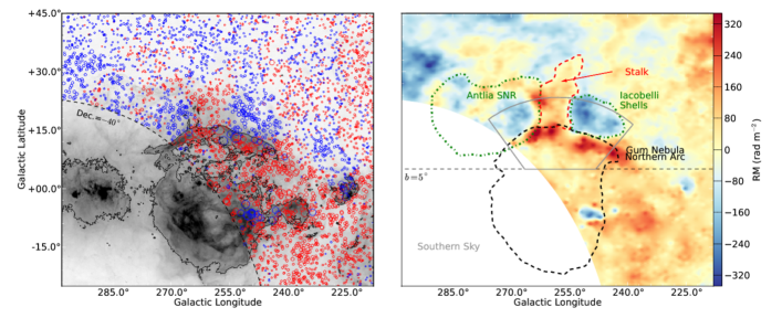
Figure 2: Left: The RM-catalogue of Taylor et al. (2009) plotted over the H $\alpha$ map of the Gum Nebula (Finkbeiner 2003). Red circles indicate positive RMs, while blue indicate negative and their diameter is proportional to $|{\rm RM}|$. The solid H $\alpha$ contour at a level of 25 R defines the outline of the nebula. Right: Prominent RM-features are easier to visualise in the map produced by Oppermann et al. (2012) using the Taylor et al. (2009) catalogue. Polygons and lines annotate significant features. We restrict our analysis to the upper arc region, inside the solid grey line.

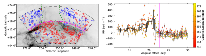
Figure 3: Left: Positions of polarised extragalactic sources selected for analysis from the Taylor et al. (2009) catalogue. Red and blue circles indicate positive and negative RMs, respectively, and the radius of each circle is scaled to the absolute value of the RM. The green dashed lines enclose regions where sources have been excised from the sample because they likely probe a contaminating region, or are obvious outliers ($>3\sigma$). Right: RMs plotted as function of angular offset from the centre of the nebula. The formal uncertainties in the catalogue are represented by vertical grey lines (scaled $\times 2$ for clarity) and each point is colour-coded for Galactic Longitude. The solid black histogram represents a median-binned version of the plot, with bin-sizes of $0.6\mbox{${}^{\circ}$}$. The solid grey histogram illustrates the level of the RMs exterior to the nebula before the discrete object correction was applied. Vertical black error-bars illustrate the $1\sigma$ scatter in each bin. The magenta line in both panels indicates the outer boundary of the nebula. In both panels the RMs are plotted assuming a flat background, i.e., no correction has been made for a large-scale RM-gradient due to the Galaxy in the background (or foreground). The effect of subtracting different model backgrounds is illustrated in Fig. 4 and discussed in $\S\ref{sec:RMs_selected}$.

Rotation measures of polarised background radio-galaxies provide a convenient method of measuring the line-of-sight magnetic field $B_{||}$ in local Galactic structures, if the electron density $n_{e}$ and the distribution of the ionised gas are known. Each extragalactic point source is effectively at infinity and the measured difference between RMs of adjacent sources is dominated by local changes in $B_{||}$ or $n_{e}$ along the line-of-sight path. The effective RM contribution of a Galactic H II region, for example, can be found by measuring the RMs of radio-galaxies behind the HII region and subtracting an average off-source RM, determined from the radio-galaxies in the surrounding sky (e.g., Harvey-Smith et al. 2011).

At the present time the best sampled and most accurate large-scale RM-grid covering a large part of the Gum Nebula is the catalogue created by Taylor et al. (2009) from the NVSS (Condon et al. 1996). NVSS radio-continuum observations were conducted on the Very Large Array (VLA) at a frequency of 1.4 GHz and extend south to a declination of $-40\mbox{${}^{\circ}$}$. The original survey combined simultaneous snapshot observations in two 42 MHz-wide bands (1364.9 MHz and 1435.1 MHz) into a multi-frequency synthesis image of the sky in Stokes I, Q, U and V. Taylor et al. (2009) reprocessed the NVSS visibility data into individual images of the bands and calculated two-channel rotation measures for 37,543 polarised sources.

2.2.1 RMs through the Gum Nebula

Fig. 2 - left presents RMs from the Taylor et al. (2009) catalogue over-plotted on the H $\alpha$ image of the Gum Nebula. Although the lower left of the nebula is not covered by the NVSS, there are RM measurements towards the upper right with source densities varying between 1.2 and 6.6 deg^-2 (Stil & Taylor 2007). It is easier to visualise RM-features in the smoothed map created by Oppermann et al. (2012) mainly from the Taylor et al. (2009) catalogue and plotted in Fig. 2 - right. Using the H $\alpha$ and radio continuum maps as a guide, we identify structures in the RM map likely associated with Galactic objects. The RM-signature of the Gum Nebula is clearly different from the background and matches the morphology of the excited hydrogen gas well. The distinctive upper arc of the nebula displays consistently positive RMs, which decrease in magnitude towards the geometric centre, reminiscent of a limb-brightened shell. The net positive RM signal in the upper Gum Nebula implies a coherent magnetic field on scales of $\sim 260$ pc, the projected diameter of the nebula at the adopted distance of $d=450$ pc. The region along the Galactic mid-plane ($|b|\lesssim 5\mbox{${}^{\circ}$}$) is highly confused, containing several H II regions and supernova remnants (see Fig. 1), while the lower part of the nebula also contains the IRAS Vela Shell, which may be a separate foreground object. In contrast, the upper part of the Gum Nebula appears relatively free of obscuring objects and we focus on this region for the remainder of the paper. The grey wedge-shaped box in Fig. 2 outlines the data selected for analysis. The selected region includes the upper arc of the nebula, the interior above $b=5\mbox{${}^{\circ}$}$ and a section of off-source RMs outside of the nebula’s border.

2.2.2 Isolating the RM-signature of the Gum Nebula

Any analysis of the RM data relies on isolating the RM-signature of the Gum Nebula from discrete regions of magneto-ionic material along the line of sight (e.g., overlapping supernova remnants or H II regions) and from the bulk of the Galaxy in the background. We have identified three other sets of discrete Galactic objects towards the upper Gum Nebula that have Faraday rotation signatures in the Taylor et al. (2009) RM-catalogue. The Antlia SNR (McCullough et al. 2002, annotated in Fig. 2) is adjacent to the nebula on the upper left. The edge of the SNR is traced by sources with RM values $10-15\,\mbox{rad\,m${}^{-2}$}$ more positive than their surroundings. This excess RM signal is comparable to the formal error in the catalogue ($\sim 12\,\mbox{rad\,m${}^{-2}$}$) and is negligible compared to RMs through the rim of the Gum Nebula ($\sim 300\,\mbox{rad\,m${}^{-2}$}$). RMs through the interior of the Antlia SNR are consistent with the background, except for a patch directly bordering the Gum Nebula, which is more negative than the large scale background by approximately $-30.0\,\mbox{rad\,m${}^{-2}$}$. This patch lies inside our selection box so we subtract this offset from RMs inside the patch to correct the catalogue. The second obvious feature in the data is a pair of shells discovered by Iacobelli et al. (2014) in 2.3 GHz radio continuum data, seen in polarisation and lying to the upper-right of the Gum Nebula. The border of the shells seen in the radio data corresponds exactly to the morphology of a negative patch of RMs in Fig. 2. We again correct the catalogue by subtracting the median background offset ($-77.2\,\mbox{rad\,m${}^{-2}$}$) from RMs inside the shell boundaries. The final feature of note is a ‘stalk’ of positive RMs extending from the centre of the upper arc to higher Galactic latitudes. The ‘stalk’ has a counterpart in H I emission identified by Reynoso & Dubner (1997), lies above a hole in the H $\alpha$ image and is hypothesised by the authors to be a ‘blowout’ in the shell wall leading to ionised gas streaming into the Galactic halo. Modelling and subtracting the signature of this feature is beyond the scope of this work, so we simply mask off the RM data within its boundary. Fig. 3 - left presents the corrected RM catalogue within the selection box, plotted over the H $\alpha$ image. The azimuthally-averaged RM-profile is shown in Fig. 3 - right). The black histogram shows a version of the profile binned in $0.6\mbox{${}^{\circ}$}$ increments. Outside of the nebula border (offsets $\gtrsim 22\mbox{${}^{\circ}$}$) the RMs are relatively constant but rise rapidly to a peak just inside the border. At smaller offsets the RM values fall slowly, approaching an interior level that is higher than the background. The grey histogram, shows the same binned profile prior to correcting for discrete contaminating sources. Note that the RM data shown here have not yet been corrected for large-scale gradients due to diffuse thermal electrons distributed throughout the bulk of the Galaxy in the background.

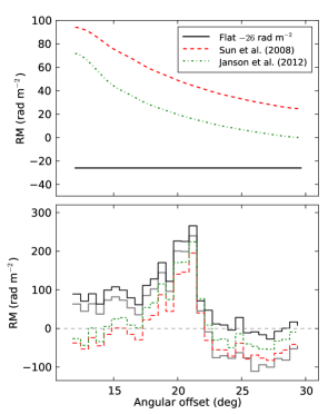
Figure 4: Top: Sample profiles at $l=259\mbox{${}^{\circ}$}$ from the models of Sun et al. (2008) and Jansson & Farrar (2012) illustrating the predicted RM-gradient with Galactic latitude. Bottom: The light-grey histogram is the azimuthally averaged RM-profile of the Gum Nebula uncorrected for discrete contaminating sources or large-scale RM background (also plotted in Fig. 3). The black histogram is the equivalent with discrete corrections applied and a flat background of $-26.4\,\mbox{rad\,m${}^{-2}$}$ subtracted. The red (dashed) and green (dot-dashed) histograms illustrate the effect of subtracting the 2-D Sun et al. (2008) and Jansson & Farrar (2012) RM-models, respectively, from each point source select from the Taylor et al. (2009) catalogue. Note that the discrete corrections have previously been applied. In both cases the large-scale gradient correction acts to decrease the RMs in the interior of the nebula relative to the exterior.

The distribution of electrons within the Galaxy and the strength, and geometry, of the ordered Galactic magnetic field result in a unique pattern of RMs over the whole sky. In the all-sky RM map compiled by Oppermann et al. (2012) the dominant signal is quadrupolar in shape, with negative RMs above and positive below the Galactic mid-plane in the vicinity of the Gum Nebula. In recent years several authors have modelled the ordered Galactic field by combining data from extra-galactic RMs and radio-synchrotron emission (Sun et al. 2008; Jansson et al. 2009; Sun & Reich 2010; Mao et al. 2010; Jaffe et al. 2010; Van Eck et al. 2011; Jansson & Farrar 2012), and explain the pattern as being due to the toroidal field in the halo. Within the Galactic disk the magnetic field and thermal electron density follow the spiral arms, increasing towards the mid-plane, leading to steep gradients in RM at low Galactic latitudes (Simard-Normandin & Kronberg 1980; Cordes & Lazio 2002; Gaensler et al. 2008). The sparse sampling of the Taylor et al. (2009) RM-catalogue and confusion towards the mid-plane mean that accurately removing the large-scale RM-signal due to the Galaxy is challenging. We initially attempted to fit a 2D polynomial surface to the off-source RMs, but this proved to be highly unreliable in practice. Instead we consider two classes of potential RM backgrounds. In the first case we assume a simple flat background at the median level of the selected RMs outside the boundary of the Gum Nebula: $-26.4\,\mbox{rad\,m${}^{-2}$}$. This assumption is the simplest correction possible and consistent with the high-latitude RM-data. However, we know that the volume-averaged electron density decays exponentially with height above the mid-plane (Cordes & Lazio 2002; Gaensler et al. 2008), thus the RMs must decrease correspondingly. Sun et al. (2008) and Jansson & Farrar (2012) have modelled the large scale RMs distribution of the Galaxy starting from the NE2001 electron density distribution and applying the scale height corrections of Gaensler et al. (2008). Both models have similar latitude profiles, illustrated for $l=258\mbox{${}^{\circ}$}$ in Fig. 4 - top. The bottom panel of Fig. 4 shows the effect of subtracting each 2-D model from the selected RM data-points. The resulting azimuthal profile is essentially the same for both models, but offset in RM as the models differ in their absolute calibration. Both models act to decrease the value of RMs towards the interior of the nebula. Neither model correctly predicts the absolute zero-level exterior to the Gum Nebula, likely because the best-fitting models are constrained over the whole sky and by other, sometimes contradictory, datasets. The authors also had limited knowledge of local contaminating objects. We adopt the RM-models of Sun et al. (2008) and Jansson & Farrar (2012) as the best available estimates of the large-scale background variation in RM and apply offsets of $-64.0\,\mbox{rad\,m${}^{-2}$}$ and $-36.6\,\mbox{rad\,m${}^{-2}$}$, respectively, so as to correct their calibration to the zero-point exterior to the Gum Nebula. In our analysis of the RMs through the Gum Nebula we compare the results derived with each of these backgrounds separately.

2.3 2.3 GHz radio continuum

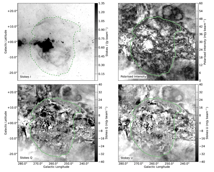
Figure 5: 2.3 GHz radio-continuum maps of the Gum Nebula from the S-PASS project. The data are calibrated in Janskys and may be converted to a main-beam brightness temperature scale in Kelvin by multiplying by 0.55. The border of the nebula traced by the green line is the same as in Fig. 2.

Radio continuum at centimetre wavelengths traces gas emitting via both synchrotron and thermal processes. If information on the polarisation state of the radiation is available, analysis of the Stokes Q and U parameters can constrain conditions in the gas along the line-of-sight, e.g., depolarisation due to a fluctuating component of the magnetic field.

The S-band Polarisation All Sky Survey (S-PASS) has imaged the entire southern sky (${\rm Dec.}<-1\mbox{${}^{\circ}$}$) in polarisation at a frequency of 2.3 GHz. The observations have been conducted with the Parkes Radio Telescope, NSW Australia, a 64-m telescope operated by CSIRO Astronomy and Space Science. A description of S-PASS observations and analysis is given in Carretti et al. (2010) and Carretti et al. (2013b). Here we report a summary of the main details. The standard S-band receiver of the observatory (Galileo) was used with a system temperature $T_{\rm sys}=20$ K, beam width FHWM$=8.9^{\prime}$ at 2300 MHz and a circular polarisation front–end ideal for linear polarisation measurements with a single-dish telescope. Data have been detected with the Digital Filter Banks mark 3 (DFB3) with full Stokes capabilities recording the two autocorrelation (RR and LL) and the complex cross-correlation products of the two circular polarisations (RR, LL, LR, RL^∗). Flux calibration was done with PKS B1934$-$638, secondary calibration with PKS B0407$-$658 and polarisation calibration with PKS B0043-424. Data were binned in 8 MHz channels and, after RFI flagging, 23 sub-bands were used, covering the ranges 2176-2216 and 2256-2400 MHz, for an effective central frequency of 2307 MHz and bandwidth of 184 MHz.

The observing strategy is based on long azimuth scans taken towards the East and the West at the elevation of the south celestial pole at Parkes (EL$=33\mbox{${}^{\circ}$}$) to realise absolute polarisation calibration of the data. Final maps are convolved to a beam of FWHM$=10.75^{\prime}$. Stokes I, Q, and U sensitivity is better than $1.0\,\mbox{mJy\,beam${}^{-1}$}$ per beam-sized pixel everywhere in the covered area. Details of scanning strategy, map-making, and final maps obtained by binning all frequency channels are presented in Carretti et al. (2010) and Carretti et al. (2015, in preparation). The confusion limit is 6 mJy in Stokes I (Carretti et al. 2013a) and much lower in polarisation (average polarisation fraction in compact sources is lower than 2 percent, Tucci et al. 2004). The instrumental polarisation leakage is 0.4 percent on-axis (Carretti et al. 2010) and less than 1.5 percent off-axis. For diffuse emission, the latter is generally not important because of cancellation effects at scales larger than the beam (e.g., Carretti et al. 2004; O’Dea et al. 2007).

2.3.1 The Polarised Signature of the Gum Nebula

Fig. 5 presents the 2.3 GHz radio-continuum image of the Gum Nebula in Stokes I, Q, U and polarised intensity $P$. The morphology of the nebula in total intensity is broadly similar to the H $\alpha$ map presented in Fig. 1, implying that the radio- and optical-emission are coming from the same gas. When viewed in P, Q and U, the upper shell of the nebula is seen to depolarise background emission in a $\sim 2\mbox{${}^{\circ}$}$ wide arc. This band of depolarisation is set against the smooth Galactic background, visible in the upper-right quadrant of the image, above $b=12\mbox{${}^{\circ}$}$. At high latitudes the background is also depolarised by two thin shells (Iacobelli et al. 2014, see $\S\ref{sec:RMs_selected}$ and Fig. 2) and by the Antlia supernova remnant in the upper-left quadrant. The shell of the Antlia SNR is similarly characterised by a band of depolarisation that overlaps the Gum Nebula at $(l,b)\approx(268\mbox{${}^{\circ}$},+13\mbox{${}^{\circ}$})$. The interiors of the Gum Nebula and Antlia SNR appear fractured, exhibiting patches of homogeneous polarised intensity interspersed with depolarised ‘canals’. The Vela supernova remnant at $(l,b)\,=\,(267\mbox{${}^{\circ}$},-3\mbox{${}^{\circ}$})$ is the brightest object in the field, ($I$ & $P$), while the rest of the Galactic plane is seen as a mix of polarised foreground and depolarised background emission.

2.4 Pulsars

The ATNF Pulsar Catalogue (APC, Manchester et al. 2005) collates the properties of more than 2300 rotation-powered pulsars and is continually revised as new discoveries are made. Of primary interest to us are the dispersion measures (DMs), RMs and distances to the pulsars. These parameters can be combined with EMs and a geometric model to derive the average electron density, filling factor and magnetic field strength along the line-of-sight.

Table 1: Properties of selected pulsars towards the Gum Nebula.

(1)	(2)	(3)	(4)		(5)		(6)	(7)
Name	$l$	$b$	DM		RM		$D$	Notes
	(deg.)	(deg.)	(${\rm cm^{-3}\,pc}$)		(${\rm rad\,m^{-2}}$)		(kpc)
Pulsars towards the upper Gum Nebula:
J0758-1528	234.464	07.224	63.327 $\pm$	0.003	55 $\pm$	7	3.72	Out
J0818-3049	249.983	02.908	133.7 $\pm$	0.2	–		4.17	Gum
J0820-1350	235.890	12.595	40.938 $\pm$	0.003	$-$1.2 $\pm$	0.4	1.9†	Out
J0828-3417	253.965	02.561	52.2 $\pm$	0.6	59 $\pm$	3	0.5	Gum
J0838-2621	248.807	08.981	116.9 $\pm$	0.1	86 $\pm$	13	4.6	Gum
J0846-3533	257.190	04.710	94.16 $\pm$	0.11	144 $\pm$	8	1.4	Gum
J0855-3331	256.847	07.517	86.635 $\pm$	0.016	165 $\pm$	10	1.2	Gum
J0900-3144	256.162	09.486	75.702 $\pm$	0.010	–		0.8	Gum
J0904-4246	265.075	02.859	145.8 $\pm$	0.5	284 $\pm$	15	4.4	Gum
J0908-1739	246.119	19.850	15.888 $\pm$	0.003	$-$31 $\pm$	4	0.6	Out
J0912-3851	263.165	06.584	70 $\pm$	1	–		0.6	Gum
J0923-31	259.697	13.003	72 $\pm$	20	–		1.0	Gum
J0932-3217	261.277	14.069	102.1 $\pm$	0.8	–		3.8	Gum
J0934-4154	268.361	07.411	113.79 $\pm$	0.16	–		3.2	Gum
J0941-39	267.795	09.904	78.2 $\pm$	2.7	–		1.3	Gum
J0945-4833	274.199	03.674	98.1 $\pm$	0.3	–		2.7	Out
J0952-3839	268.702	12.033	167 $\pm$	3	–		8.4	Gum, Ant
J0959-4809	275.742	05.418	92.7 $\pm$	1.2	50 $\pm$	6	3.0	Out
J1000-5149	278.107	02.603	72.8 $\pm$	0.3	46 $\pm$	9	2.3	Out
J1003-4747	276.037	06.117	98.1 $\pm$	1.2	18 $\pm$	4	3.4	Out
J1012-2337	262.131	26.377	22.51 $\pm$	0.09	52 $\pm$	9	1.3	Out
J1032-5206	282.354	05.128	139 $\pm$	4	–		4.3	Out
J1034-3224	272.050	22.117	50.75 $\pm$	0.08	$-$8 $\pm$	1	4.7	Ant
J1036-4926	281.518	07.727	136.529 $\pm$	0.010	$-$11 $\pm$	6	8.7	Out
J1045-4509	280.851	12.254	58.166 $\pm$	0.001	92 $\pm$	1	0.23†	Ant
J1057-4754	284.007	10.739	60 $\pm$	8	–		3.0	Ant
J1105-43	283.511	14.886	38.000 $\pm$	0.001	–		2.2	Ant
Pulsars below $b=2\mbox{${}^{\circ}$}$ with accurate distances:
J1001-5507	280.226	00.085	130.32 $\pm$	0.17	297 $\pm$	18	0.3†	Out
J0737-3039B	245.236	$-$4.505	48.920 $\pm$	0.005	112.3 $\pm$	1.5	1.1†	Out
J0738-4042	254.194	$-$9.192	160.8 $\pm$	0.7	12.1 $\pm$	0.6	1.6†	Gum
J0742-2822	243.773	$-$2.444	73.782 $\pm$	0.002	149.9 $\pm$	0.1	2.0†	Out
J0835-4510	263.552	$-$2.787	67.99 $\pm$	0.01	31.4 $\pm$	0.1	0.28†	Gum
J0837-4135	260.904	$-$0.336	147.29 $\pm$	0.07	135.8 $\pm$	0.3	1.5†	Gum
J0908-4913	270.266	$-$1.019	180.37 $\pm$	0.04	10.0 $\pm$	1.6	1.0†	Gum
J0942-5552	278.571	$-$2.230	180.2 $\pm$	0.5	-61.9 $\pm$	0.2	0.3†	Out

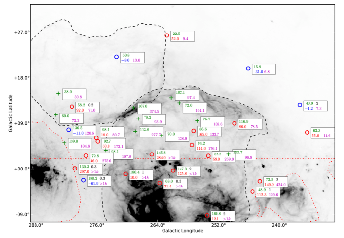
Figure 6: Selection of pulsars with known DM values towards the Gum Nebula. All pulsars with $b>2\mbox{${}^{\circ}$}$ are shown alongside a selection of pulsars with accurate distances below $b=2\mbox{${}^{\circ}$}$. Red dot-dashed lines outline confusing parts of the Galactic plane and pulsars in these regions have been omitted. ‘$\circ$’ symbols represent pulsars with both DM and RM measurements, and ‘$+$’ symbols pulsars with only DM measurements. Each pulsar is annotated with its DM in pc cm^-3 (top-left number, coloured green), RM in rad m^-2 (bottom-left number, coloured red or blue signifying positive or negative RM, respectively), independently determined distance in kpc, where known (top-right number, coloured black) and EM in pc cm^-6 (bottom-right number, coloured magenta).

We utilise version 1.49 of the APS, which lists 158 pulsars within a $30\,\mbox{${}^{\circ}$}$ radius of the kinematic centre of the Gum Nebula ($l=261.0\mbox{${}^{\circ}$},~{}~{}~{}b=-2.5\mbox{${}^{\circ}$}$; Woermann et al. 2001). Of these we have chosen 35 for analysis, most of which lie within the upper Gum region. Fig. 6 and Table 1 present this sample, which contains all pulsars above $b=2\mbox{${}^{\circ}$}$ and a handful below, chosen because they have accurately determined distances or lie on unconfused sight-lines adjacent to the Gum Nebula.

Accurate distances to pulsars are difficult to obtain: a handful of precise values have been calculated via annual parallaxes and these are limited to relatively nearby pulsars ($<3$ kpc). Kinematic distances accurate to $\sim 1$ kpc can be derived for some pulsars associated with H I absorption, while the distance to pulsars located in globular clusters can be estimated to $\sim 15\%$ reliability via analysis of colour-magnitude diagrams. Most of the pulsars detected towards the Gum Nebula default to a distance derived from the dispersion measure. Such DM-distances are often highly inaccurate because they rely on a model of the Galactic free-electron distribution (Cordes & Lazio 2002; Taylor & Cordes 1993), which was itself created in part using the Taylor et al. (1993) pulsar catalogue. Distances are particularly ill-determined towards the Gum Nebula, which was included in the Cordes & Lazio (2002) model as a pair of overlapping spheres of diameter 50 pc. It is not clear that this is an improvement on the older Taylor & Cordes (1993) model which treated the nebula a simple Gaussian of full width half maximum (FWHM) 50 pc truncated at $r=130$ pc. The Cordes & Lazio (2002) model does, however, account for the scatter broadening $\tau_{\rm sc}$ which was measured by Mitra & Ramachandran (2001) for 40 pulsars between $250\mbox{${}^{\circ}$}<l<290\mbox{${}^{\circ}$}$. They found that $\tau_{\rm sc}$ was greater than expected for a smooth Gaussian, implying a more inhomogeneous distribution of $n_{e}$. Based on the observed scattering they concluded that pulsars in the vicinity of the Gum Nebula should be 2 - 3 times closer than predicted by Taylor & Cordes (1993). Within the area of the Gum Nebula only four pulsars have both DM measurements and accurate distances. The Vela pulsar (J0835$-$4510) is known to be at a distance of $287^{+19}_{-17}$ pc (Dodson et al. 2003), placing it just inside the front wall of the nebula. The remaining three (J0738$-$4042, J0837$-$4135 and J0908$-$4913) lie at distances greater than 1 kpc (see the bottom of Table 1), behind the Gum Nebula.

3 Analysis

Our analysis aims to answer the questions: What is the likely origin of the Gum Nebula? and What are the magnetic properties of the nebula and how do they affect ambient conditions in this part of the Galaxy? To address these questions we construct a simple model of the nebula as an ionised shell situated in the near-field. We present the model below and explain the maximum-likelihood method used to fit the model to RMs on the sky. The model assumes a uniform density distribution plus a jump in ionisation fraction from 0 to 100 percent within the shell of the Gum Nebula, which we derive from the H $\alpha$ data and include as a prior in our fitting procedure. The resulting fits will be presented in $\S\ref{sec:results}$.

3.1 Rotation Measures as Magnetic Probes

Faraday rotation causes the polarisation angle of a linearly polarised wave traversing a magnetised ionised medium to rotate by an angle $\Delta\psi$. The change in polarisation angle is given by

$$\Delta\psi={\rm RM}\,\lambda^{2}~{}~{}~{}{\rm rad},$$ (1)

where RM is the rotation measure in radians m^-2. The observed RM depends on the line-of-sight component of the magnetic field $B_{||}$ (in $\mu$G), the thermal electron density $n_{e}$ (in ${\rm cm^{-3}}$) and the path length $dl$ (in pc) according to

$${\rm RM}=0.81~{}\int_{src}^{obs}n_{e}\,B_{||}\,dl~{}~{}~{}{\rm rad\,m^{-2}}.$$ (2)

Note that the integral in Equation 2 is taken from the source of the polarised emission to the observer, so that a positive RM indicates an average magnetic field pointing towards the observer. If the ionised material along the line-of-sight contains clumps of uniform $n_{e}$ threaded by the same $B_{||}$, then the medium is characterised by a volume filling factor $f$. Equation 2 becomes

$${\rm RM}=0.81\,n_{e}\,B_{||}\,f\,L~{}~{}~{}{\rm rad\,m^{-2}},$$ (3)

where $L$ is the total path length through the ionised medium and $f\,L$ is known as the occupation length. $L$ can generally be estimated from the geometry of the object under consideration (e.g., a slab, sphere or shell).

3.2 A Near-Field Magnetic Bubble Model

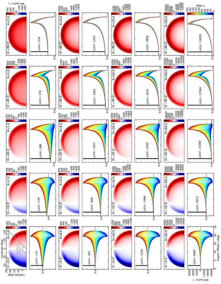
Figure 7: Grid of models showing how changes in the angle of the magnetic field $\Theta$ and the compression factor $X$ affect the distribution of RMs across a simple ionised shell. The geometry of the model is described in the Appendix (see Fig. A 1.) and the parameters are set to: $D=450$ pc, $\phi_{outer}=22.7\mbox{${}^{\circ}$}$, $dr=25.0$ pc, $n_{e}=1.7\,\mbox{cm${}^{-3}$}$, $B_{0}=8.6\,\mu$G and $f=0.5$. Each model is presented in two panels: the upper panel presents a map of RM in offset Galactic coordinates and the lower panel displays radial RM profiles extracted over a range of angles $\Upsilon$ to the Galactic plane ($0\mbox{${}^{\circ}$}\leq\Upsilon\leq 180\mbox{${}^{\circ}$}$).

Models of RMs through spherical ionised shells have recently been used to derive magnetic properties of Galactic SNRs and H II regions, and to probe the magnitude and orientation of the ordered Galactic magnetic field, e.g. Savage et al. (2013), Harvey-Smith et al. (2011), Whiting et al. (2009) and Kothes & Brown (2009). These phenomena ionise their surroundings and illuminate the ambient magnetic field via Faraday rotation. As they expand into the ISM they may also compress the field, imprinting a specific signature on the rotation measures. Previous investigations have focused on distant objects ($>1$ kpc) whose small angular diameters ($<5\mbox{${}^{\circ}$}$) mean that they intercept fewer RM sight-lines compared to the nearby Gum Nebula. Because these bubbles lie in the far-field, their RM profiles may be integrated in azimuth under the assumption of spherical symmetry. However, for a near-field bubble like the Gum Nebula, the sign and shape of the RM-profile can vary with azimuth, depending on the orientation of the ordered magnetic field.

In a similar way to Whiting et al. (2009) and Savage et al. (2013), we model the Gum Nebula as a spherical ionised shell of radius $R$ and thickness $dr$, threaded by a uniform, parallel magnetic field $\overrightarrow{B_{0}}$. We assume that the electron density $n_{e}$ is constant within the shell and zero elsewhere (i.e., the background has been removed as in $\S\ref{sec:datasets_ha}$ and the electron density in the interior of the shell is negligible). The observer is located in the near-field and the magnetic field lines make an angle $\Theta$ to the plane of the sky in the direction of the bubble centre. The tilt angle of the magnetic field is assumed fixed along the y-axis, representing the Galactic plane, and the angle $\zeta$ describes the orientation of the sight-line to the yz-plane. The edge of the shell subtends an angular radius of $\phi_{\rm outer}={\rm sin}^{-1}(R/D)$, where $D$ is the distance from the observer to the geometric centre of the shell. A full description of the adopted geometry can be found in Appendix A, including a detailed schematic.

If the shell is expanding supersonically into the ISM then the gas, and hence the magnetic field, will be compressed at the external boundary. If the expansion has slowed to sub-sonic speeds then the gas will simply move out of the way. To model the compression (or lack of) we assume the electron density behind the expansion front is given by $n_{e}=X\,n_{0}$, where $X$ is the compression factor and $n_{0}$ is the electron density in the ambient medium. At each point on the sphere the component of the magnetic field tangent to the shell ($B_{\perp}$) is amplified by $X$ while the normal component ($B_{n}$) is unaffected. The contribution to the observed magnetic field by one hemisphere is simply the vector sum of $X\,B_{\perp}$ and $B_{n}$ projected along the line of sight. The measured RM is then proportional to the sum of the ingress (far hemisphere) and egress (near hemisphere) components. Equation 3 becomes a function of polar coordinate ($\phi$, $\zeta$), compression factor $X$, electron density $n_{e}$, magnetic field strength $B_{0}$ and the angle of the magnetic field to the plane of the sky $\Theta$

$${\rm RM}=0.81\,f\,\left(\frac{B_{\rm||}(\phi,\zeta,{B_{0}},\Theta,X)}{\mbox{$\mu$G}}\right)\left(\frac{n_{e}}{\mbox{cm${}^{-3}$}}\right)\left(\frac{L(\phi,dr)}{pc}\right).$$ (4)

The model implicitly assumes that the same $B_{\rm||}$ applies everywhere along the half-chord between the outer surface and mid-plane of the shell (but different for ingress and egress). This assumption will only be realistic for a thin shell; a more sophisticated analysis is outside the scope of this paper. The model also assumes a constant value for the electron density within the shell and, because $n_{e}$, $B_{\rm los}$ and $f$ are degenerate in Equation 3, the electron density and filling factor must be estimated from independent data, if possible (see $\S\ref{sec:ne}$, below).

Fig. 7 presents a grid of near-field bubble models, illustrating how the RM observed on the sky changes as $\Theta$ and $X$ are varied. In the far-field case, the rotation-measure profile is spherically symmetric, i.e., constant with $\zeta$ (the angle between the profile sampling line and the Galactic plane, see Fig. 16). However, in the near-field case the profile shape depends on both $\zeta$ and $\Theta$ (the orientation of the ordered magnetic field vector). As $\Theta$ increases from $0\mbox{${}^{\circ}$}$ ($\overrightarrow{B_{0}}$ in the plane of the sky) to $90\mbox{${}^{\circ}$}$ ($\overrightarrow{B_{0}}$ pointing towards observer) the large scale distribution of RMs changes from being anti-symmetric to symmetric around the central latitude axis. Increasing $X$ leads to an overall increase in the magnitude of the RM and a large difference in RM between the centre and inner-edge of the shell. The shape of the profile edge also becomes more rounded because of limb-brightening, although this would be much more noticeable in far-field bubbles.

In $\S\ref{sec:fitting}$, below, we present a maximum-likelihood method used to fit the model to rotation measures from the Taylor et al. (2009) catalogue. We incorporate estimates of $n_{e}$ from H $\alpha$ data as a prior, assuming Gaussian errors.

3.3 $n_{e}$ from H $\alpha$ data

From Equation 2 we see that $n_{e}$ and $B_{||}$ are degenerate and cannot be determined individually from observations of RM alone. However, a separate observation of the emission measure provides an independent estimate of the electron density along the line of sight. EM is related to $n_{e}$ via

$${\rm EM}=\int_{0}^{\infty}n_{e}^{2}\,dl~{}~{}~{}{\rm pc\,cm^{-6}}.$$ (5)

Assuming the same clumpy medium and geometry as presented in Section 3.1 this becomes

$${\rm EM}=n_{e}^{2}\,f\,L~{}~{}~{}{\rm pc\,cm^{-6}},$$ (6)

with filling factor $f$ and path length $L$ as before. EM may be calculated directly from the intensity of the $\mbox{H\,$\alpha$}\,(3-2)$ line via the equation of Reynolds (1988)

$${\rm EM}=2.75\left(\frac{T_{e}}{10^{4}\,{\rm K}}\right)^{0.9}\left(\frac{I_{\rm H_{\alpha}}\,K}{\rm R}\right)~{}~{}~{}{\rm cm^{-6}\,pc},$$ (7)

where $T_{e}$ is the electron temperature in K, $I_{\rm H_{\alpha}}$ is the intensity of the H $\alpha$ emission in Rayleighs and $K=\tau\,/\,(1-e^{-\tau})$ is a correction term to account for dust extinction between the H $\alpha$ emission and the observer (see Section 2.1.1).

Most estimates of $T_{e}$ for the Gum Nebula within the literature vary between 6500 K and 11500 K. Electron temperatures derived by Reynolds (1976a) from a comparison of H $\alpha$ to [NII] linewidths are consistent with a uniform temperature of 11300 K throughout the nebula. However, Vidal (1979) determined the electron-temperature to be $T_{e}=6500$ K from existing optical emission-line data. We adopt a uniform value of $8000$ K for this analysis.

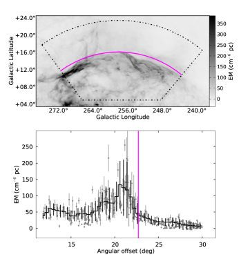
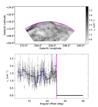
Figure 8: Left: EM map and azimuthally averaged profile of the upper Gum region. The individual grey points in the bottom panel show the EM values at the positions of the RM samples while the black points with error bars show the azimuthal average and standard-deviation in 0.2 degree bins. Right: Electron density map and azimuthal averaged profile derived assuming the best-fit parameters in Table 2. The magenta line shows the edge of the shell model.

Fig. 8 - top-left presents the emission measure map of the upper Gum region derived from the Finkbeiner (2003) H $\alpha$ data using Equation 7. Azimuthally averaged EM values peak at $220\,\mbox{pc\,cm${}^{-6}$}$ (see Fig. 8 - bottom-left), falling to $\sim 80\,\mbox{pc\,cm${}^{-6}$}$ in the interior and $\lesssim 30\,\mbox{pc\,cm${}^{-6}$}$ outside the nebula. Our values are largely consistent with those of previous authors. Reynolds (1976a) measured the EM via pointed H $\alpha$ spectral observation and found it varied from $100\,\mbox{pc\,cm${}^{-6}$}$ interior to the nebula to $240\,\mbox{pc\,cm${}^{-6}$}$ in the upper arc. Scans across the region by Reynolds (1976a) at $l=240\mbox{${}^{\circ}$}$ determined the Galactic background to be $<10\,\mbox{pc\,cm${}^{-6}$}$ rising to $28\,\mbox{pc\,cm${}^{-6}$}$ at the mid-plane.

Assuming the geometry $L(\phi,dr)$ from the best-fit to our shell model (presented in $\S\ref{sec:results}$, below) and best-fit filling factor $f=0.3$ we use Equations 6 and A2 to derive the electron density $n_{e}$ inside the clumpy shell. The electron density map and azimuthally averaged profile are presented in Fig. 8 - right. The fitting procedure takes the value of $n_{e}$ as a prior (see $\S\ref{sec:fitting}$) altering the most likely shell geometry and filling factor $f$, requiring a new estimate of $n_{e}$. To correct for this inconsistency we re-calculated $n_{e}$ using the new $L(\phi,dr)$ and $f$, and iterated over the fitting loop until all values converged. The final electron density was determined to be $n_{e}=1.4\pm 0.4\,\mbox{cm${}^{-3}$}$, which compares well with Reynolds (1976b) who found $n_{e}\approx 1\,\mbox{cm${}^{-3}$}$ in the fainter parts of the nebula, assuming fixed physical parameters ($\phi_{outer}=18\mbox{${}^{\circ}$}$, $D=450$ pc and $15\lesssim dr\lesssim 30\,$pc).

3.4 Maximum likelihood analysis

We use a Markov Chain Monte Carlo (MCMC) algorithm to fit the model shell to the RM data in the upper Gum region. The de-facto algorithm for performing MCMC fitting is the Metropolis-Hastings algorithm (Metropolis et al. 1953; Hastings 1970), which randomly samples over parameter space, accepting or rejecting models based on their likelihood $\mathcal{L}$ (i.e., the probability of the data given the model parameters). New positions with greater $\mathcal{L}$ than previously are always accepted, while those with smaller $\mathcal{L}$ are occasionally accepted. Our code makes use of the efficient affine-invariant sampler (Goodman & Were 2010) implemented in the EMCEE python module by Foreman-Mackey et al. (2013). EMCEE controls a number of parallel samplers, referred to as ‘walkers’, each of which corresponds to a vector of free parameters within the model. The walkers are initialised to a point in n-dimensional parameter space and are iteratively updated to map out the probability distribution. At each iteration the likelihood is calculated assuming Gaussian errors according to $\mathcal{L}=e^{-\chi^{2}/2}$, where $\chi^{2}$ is the standard chi-squared goodness-of-fit statistic. If priors with measured uncertainties exist for any model parameter, we incorporate them into the likelihood calculation by summing their chi-squared values $\chi^{2}=\chi^{2}_{\rm model}+{\textstyle\sum\nolimits_{i}}\,\chi^{2}_{{\rm prior}\,i}$.

The fitter is started by generating 300 walkers initialised to random values of the free parameters. The MCMC code is initially run for 400 ‘burn-in’ iterations to allow the walkers to settle in a clump around the peak in likelihood space. The fitting routine is then run for 10000 iterations to produce a well-sampled likelihood distribution. We determine the best fitting model from the mean of the marginalised posterior distribution for each free parameter. The $\pm 1\sigma$ uncertainties are calculated as the fractional positions at $1-{\rm erf}(1\sigma)=0.1572$ and ${\rm erf}(1\sigma)=0.8427$ on the normalised cumulative distribution. Our results are presented in $\S\ref{sec:results_fit}$

3.4.1 Scatter in RM as a hyperparameter

The median measurement uncertainty on the selected RM data is $\sigma({\rm RM})=12\,\mbox{rad\,m${}^{-2}$}$, considerably smaller than the scatter evident in Fig. 3 - right. The error-bars reflect only the uncertainty in the measurement and do not take into account systematic scatter, e.g., due to fluctuations in $B_{||}$ or $n_{e}$ on scales much smaller than the sampling grid, or systematic errors in RM determination. We characterise this additional variation using a term $\delta({\rm RM})$ added in quadrature to the measurement uncertainty. This new scatter term is included in the model as a free parameter, however, it is treated slightly differently when calculating the likelihood function.

Lahav et al. (2000) and Hobson et al. (2002) present a formalism for performing joint analysis of cosmological datasets by introducing hyperparameter weighting terms, the values of which are determined directly from the statistical properties of the data. This approach is easily adapted to find the self-consistent uncertainties for data with ill-determined error-bars. Using Equations 29 and 30 of Hobson et al. (2002) we calculate a likelihood function using the modified chi-squared statistic

$${\rm\chi^{2}=\sum_{i}\left[\,\frac{(RM_{i}-RM_{mod})^{2}}{\sigma(RM)_{tot,i}^{2}}+{\rm ln}(2\,\pi\,\sigma(RM)_{tot,i}^{2})\,\right]},$$ (8)

where ${\rm RM_{i}-RM_{mod}}$ is the difference between the ${\rm i^{th}}$ rotation measure and the model at that position. The second term inside the parentheses is required to correctly normalise the likelihood and the total uncertainty on the ${\rm RM_{i}}$ is given by

$${\rm\sigma(RM)_{tot,i}^{2}=\sigma(RM)_{i}^{2}+exp[\,2\,ln(\,\delta(RM)_{i}\,)\,]}.$$ (9)

Here we solve for ${\rm ln(\,\delta(RM)\,)}$ rather than directly for ${\rm\delta(RM)}$ so as to enforce positivity in the scatter term (i.e., uncertainties cannot be negative).

4 Results

4.1 General comparison of model and data

Before presenting the results of the MCMC analysis, it is useful to visually compare the RM data shown in Fig. 3 with the simple shell models illustrated in Fig. 7. Two key discriminators stand out in the behaviour of the models. Firstly, the difference in rotation measure between the interior and the peak of the shell (${\rm\Delta RM}$, illustrated by the black line in Figures 7) is a strong function of the compression factor $X$, assuming other parameters are fixed. From Fig. 3 - right we see that the measured ${\rm\Delta RM}$ in the profile of the northern Gum Nebula is $\sim 350\,\mbox{rad\,m${}^{-2}$}$, restricting the compression factor to $X\lesssim 4$. Models with higher values of $X$ result in much greater ${\rm\Delta RM}$ for all reasonable values of $n_{e}$, $f$, $B_{0}$ and $\Theta$. Secondly, the longitudinal RM-gradient is directly related to the pitch angle of the magnetic field. This behaviour is due to the close proximity of the nebula, so that sight-lines from opposite sides are not parallel and intersect a uniform field at different angles. If the ordered magnetic field is directed along the plane of the sky at the nebula’s centre ($\Theta=0\mbox{${}^{\circ}$}$), we would expect to measure equal positive and negative RMs on either side of the central longitude. For a magnetic field pointing directly towards ($\Theta=90\mbox{${}^{\circ}$}$) or away ($\Theta=-90\mbox{${}^{\circ}$}$) from the Sun the RMs would display symmetric positive or negative patterns, respectively. We see mostly positive RMs towards the Gum Nebula, with a slight positive gradient towards lower Galactic longitudes (see Fig. 3). From an examination of the grid of models shown in Figure 7, we can conservatively state that the ordered magnetic field is pointing towards the Sun at an angle $\Theta\gtrsim 20\mbox{${}^{\circ}$}$. This is because the negative peak in RMs at positive Galactic longitudes is absent from models with $\Theta\gtrsim 20\mbox{${}^{\circ}$}$, and from the Taylor et al. (2009) RMs. In $\S\ref{sec:results_fit}$ below we quantify these assertions using fits to the data.

4.2 Fits to the model shell

Here we present the results of fitting the model described in $\S\ref{sec:mag_bubble}$ to a subset of the Taylor et al. (2009) RM catalogue. The RM data included in the fit are outlined by the wedge-shaped box in Fig. 3 - left and was selected to bracket the nebula above $b>5\mbox{${}^{\circ}$}$ (excluding the ‘stalk’ region and a handful of negative outliers - see $\S\ref{sec:RMs_selected}$). We fixed the centre of the model to $(l,\,b)=(258.0\mbox{${}^{\circ}$},\,-6.6\mbox{${}^{\circ}$})$ so that the circumference of the shell corresponds to the sharp outer edge seen in the H $\alpha$ data (see Fig. 1). The mean of the marginalised likelihood distribution is a good estimator of the best fitting value for each parameter; these are reported in Table 2 and described below.

Table 2: Results of fitting the ionised shell model to the RM catalogue.

(1)	(2)	(3)	(4)	(5)			(6)			(7)
Parameter	Symbol	Unit	Notes	Assumed Background Level
				Flat			Sun et al. (2008)			Jansson & Farrar (2012)
Distance	$D$	pc	Fixed		450			450			450
Background RM	${\rm RM_{bg}}$	rad m-2	Fixed		$-26.4$			$-64.0$			$-36.6$
Filling factor	$f$	–	Free		0.4	${}^{+0.3}_{-0.2}$		0.3	${}^{+0.3}_{-0.1}$		0.2	${}^{+0.2}_{-0.1}$
Angular radius	$\phi_{\rm outer}$	deg.	Free		22.7	${}^{+0.2}_{-0.1}$		22.7	${}^{+0.1}_{-0.1}$		22.7	${}^{+0.1}_{-0.1}$
Shell thickness	$dr$	pc	Free		20.2	${}^{+1.8}_{-1.6}$		18.5	${}^{+1.5}_{-1.4}$		18.5	${}^{+1.3}_{-1.3}$
Field angle	$\Theta$	deg.	Free		55	${}^{+15}_{-12}$		43	${}^{+13}_{-9}$		55	${}^{+16}_{-12}$
Field strength	$B_{0}$	$\mu$G	Free		8.8	${}^{+6.1}_{-4.0}$		3.9	${}^{+4.9}_{-2.2}$		3.9	${}^{+4.2}_{-2.1}$
Compression factor	$X$	–	Free		1.1	${}^{+0.5}_{-0.3}$		6.0	${}^{+5.1}_{-2.5}$		6.8	${}^{+5.3}_{-2.8}$
Electron density	$n_{e}$	${\rm cm^{-3}}$	Prior		1.4	${}^{+0.4}_{-0.4}$		1.3	${}^{+0.4}_{-0.4}$		1.2	${}^{+0.4}_{-0.4}$
Additional RM Scatter	$\delta({\rm RM})$	rad m-2	Free		75.1	${}^{+2.9}_{-2.7}$		71.0	${}^{+2.7}_{-2.7}$		70.0	${}^{+2.9}_{-2.6}$

We initially ran our MCMC fitting procedure assuming a flat, large-scale background of ${\rm RM_{bg}=-26.4\,\mbox{rad\,m${}^{-2}$}}$ and with all other parameters free, except distance, which was fixed at $D=450$ pc and electron density, for which a prior of $n_{e}=1.4\pm{0.4}\,\mbox{cm${}^{-3}$}$ was set (see $\S\ref{sec:ne}$). Likelihood distributions $\mathcal{L}$ and plots of RM are presented in Fig. 9. The triangular matrix of confidence contour plots illustrates how the free parameters interrelate, while the histograms on the diagonal show the marginalised likelihood distributions for individual parameters. Of particular note are the distributions for $f$, $n_{e}$, $B_{0}$, $dr$ and $X$. The likelihood distribution for the filling factor is very broad, only constraining $f\gtrsim 0.25$, below which the marginalised distribution drops off rapidly. The curved and elongated confidence contours between $B_{0}$ and $f$ mean that these two parameters are highly degenerate, and that the strength of the magnetic field is not well determined in the absence of an independent estimate of $f$. The prior on electron density has the effect of constraining the likely range of $n_{e}$ values and eliminates most of the degeneracy between $n_{e}$ and $B_{0}$. Confidence contours between $dr$ and $\theta_{\rm outer}$ are elliptical in shape, indicating that the RM-data do not pinpoint the radius and thickness of the shell independently. Nonetheless, the range of values for each parameter is small and their absolute values are well constrained. The marginalised $\mathcal{L}$ distribution for the compression factor $X$ exhibits a narrow profile centred on 1.1, implying that the gas within the shell has not been significantly compressed. The hyperparameter characterising the additional scatter on the RMs is well determined at $\delta({\rm RM})=75.1^{+2.9}_{-2.7}\,\mbox{rad\,m${}^{-2}$}$, as shown by the Gaussian form of its marginalised likelihood distribution. By definition the hyperparameter procedure adjusts $\delta({\rm RM})$ so that $\chi^{2}=1.0$, thus $\delta({\rm RM})$ can be though of as a proxy for $\chi^{2}$ when comparing ‘goodness-of-fit’ between models.

We ran the MCMC analysis again after correcting the data for the large-scale RM-gradients modelled by Sun et al. (2008) and Jansson & Farrar (2012). The shape of the gradients is similar for both modes (illustrated in Fig. 4) and removing these backgrounds has the effect of decreasing the RM-values towards lower Galactic latitudes. Due to the orientation of the selection box, this results in a decreased RM-signal towards the centre of the Gum Nebula compared to the edge. The parameters of the best-fitting models to the gradient-subtracted versions of the RM-catalogue are presented in columns (6) and (7) of Table 2, and illustrated in Figs. 10 and 11. The results of both MCMC fits are identical within the errors, so we refer to the version assuming the Sun et al. (2008) background in the following discussion.

Comparing the results of fits to the flat- and gradient-subtracted data, the most significant difference is in the compression factor $X$, whose value changes from $1.1^{+0.5}_{-0.3}$ to $6.0^{+5.1}_{-2.5}$, respectively. This change is purely a result of the smaller difference between RMs in the interior of the nebula and the peak. $X$ is much less well constrained by the gradient-subtracted data as the difference between the interior and exterior levels approaches the scatter on the data. The confidence contours in Fig. 10 also show that $X$ is more degenerate with $f$ and $B_{0}$. The higher compression factor is balanced by corresponding small decreases in filling factor $f$, shell thickness $dr$, field strength $B_{0}$ and electron density $n_{e}$. The filling factor $f$ is slightly better constrained, leading to a correspondingly more precise value for $B_{0}=3.9^{+4.9}_{-2.2}\,\mbox{$\mu$G}$. The uncertainties on fitted values of magnetic field angle $\Theta$ are large (typically $\sim 12\mbox{${}^{\circ}$}$), however, the fitted angles are broadly similar for all three fits. The value of $\delta({\rm RM})$ is lower by $4.1\,\mbox{rad\,m${}^{-2}$}$ in the gradient-subtracted fit, implying that the model is a better match to this data. However, the absolute change is equivalent to only $\sim 1.5\sigma$ between the two MCMC runs. We discuss the implications of the results in $\S\ref{sec:discussion}$.

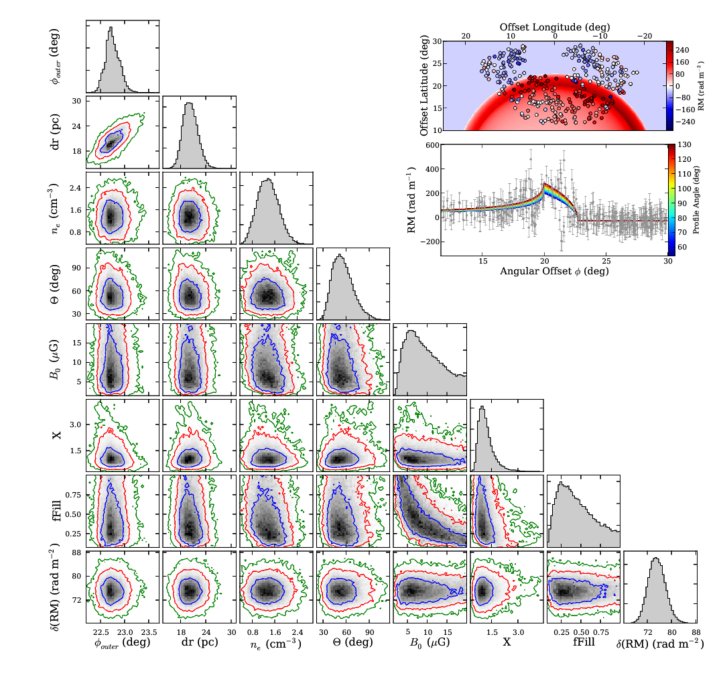
Figure 9: Main-figure: Triangular grid of confidence plots for the Gum Nebula, produced by fitting the ionised shell model to the Taylor et al. (2009) RM-catalogue assuming a flat background (also see Table 2). The blue, red and green contours represent the $1\sigma$, $2\sigma$ and $3\sigma$ confidence intervals, respectively. The filled histograms on the diagonal show the marginalised likelihood distributions for each free parameter in the model. Inset: The rotation measure image (top) and azimuthal profile (bottom) for the best fitting model over-plotted by the selected RM data from the Taylor et al. (2009) catalogue. Note the compressed range in angular offset on the x-axis of the inset panel, compared to the equivalent plots in Fig. 7.

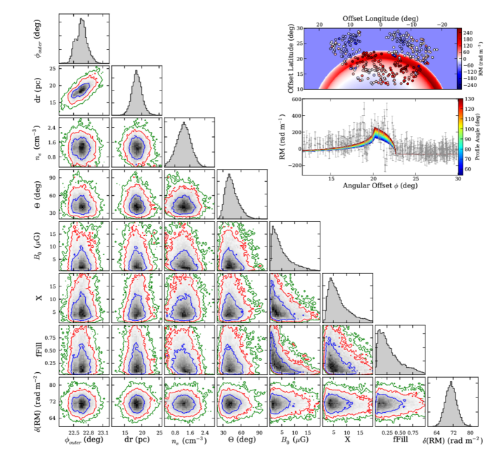
Figure 10: As for Fig. 9, but assuming a background as given by Sun et al. (2008).

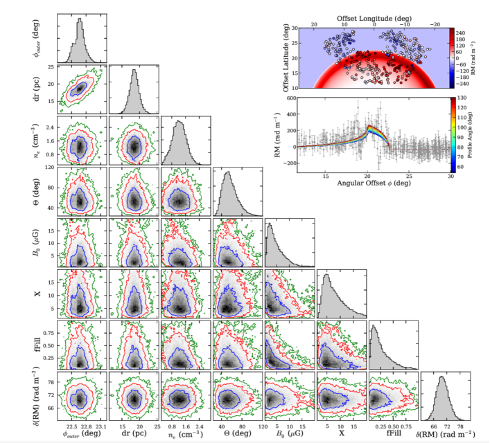
Figure 11: As for Fig. 9, but assuming a background as given by Jansson & Farrar (2012).

4.2.1 Consistency checks - pulsars

Although fewer in number than extragalactic sources, pulsars with well determined distances are useful in checking the results of an extragalactic RM or EM analysis. The interaction between free electrons and photons introduces a differential time delay $\Delta t$ across the observational bandwidth $\Delta\nu$. The delay is a function of frequency $\nu$ and is characterised by the dispersion measure according to $(\Delta t/\mu s)=8.3\,\Delta\nu\,({\rm DM}/cm^{-3}\,pc)\,\nu^{-3}$, where all frequencies are in GHz. The measured DM of a pulsar is related to the electron density via

$${\rm DM}=\int_{obs}^{psr}n_{e}\,dl~{}~{}~{}{\rm cm^{-3}\,pc}.$$ (10)

Assuming the same volume filling factor $f$ and path length $L$ as before, Equation 10 can be written as

$${\rm DM}=n_{e}\,f\,L~{}~{}~{}{\rm cm^{-3}\,pc}.$$ (11)

With suitable observations and by combining Equations 3, 6 and 11 we can solve for $f$, $B_{||}$ or $n_{e}$ along the line-of-sight to a pulsar. For example, the average line-of-sight magnetic field strength is given by $B_{||}=\frac{\rm RM}{\rm 0.81\,DM}$, the electron density inside the clumps by $n_{e}=\frac{\rm EM}{\rm DM}$ and the filling factor by $f=\frac{\rm DM^{2}}{{\rm EM}\,L}$.

The RMs, DMs and accurate distances (where available) of selected pulsars towards the upper Gum region have been presented in Fig. 6. A few general trends are worth noting: on average the DMs increase towards the Galactic mid-plane as the electron density peaks at $b\approx 0\mbox{${}^{\circ}$}$ (Gaensler et al. 2008). After taking the latitude dependence into account, the DMs of pulsars towards the nebula appear to be enhanced when compared to sight-lines outside of its border. Typically, pulsar sight-lines just inside shell edge have DMs of 100 – 150 pc cm^-3 compared to 20 – 60 pc cm^-3 outside. The DM of the Vela pulsar (J0835$-$4510) is 68 pc cm^-3, greater by 19 pc cm^-3 compared to the pulsar J0737$-$3039A, which lies just outside the nebula at distance of 1.1 kpc. The difference is representative of how much dispersion is created by one wall of the nebula.

The clumpy electron density derived from $n_{e}=\frac{\rm EM}{\rm DM}$ using only pulsars above $b>5\mbox{${}^{\circ}$}$ inside the nebula varies from $0.7\,\mbox{cm${}^{-3}$}$ to $2.2\,\mbox{cm${}^{-3}$}$ with an average of $1.5\,\mbox{cm${}^{-3}$}$. Outside the nebula, but away from the plane, $n_{0}$ (i.e., the ambient value) falls to values of $0.2\,\mbox{cm${}^{-3}$}$ to $0.9\,\mbox{cm${}^{-3}$}$. Given the large uncertainties these values are in agreement with our best-fitting models.

Only a handful of pulsars inside the nebula have both RMs and DMs, allowing the determination of the average line-of-sight magnetic field strength $B_{||}$. Three pulsar sight-lines intersect the upper Gum region, away from the shell, and their DM values suggest they lie beyond the nebula. Values for $B_{||}$ derived from the pulsars range between $0.9\,\mbox{$\mu$G}$ and $2.4\,\mbox{$\mu$G}$, significantly lower than the best-fit value to the flat-background data ($8.8^{+6.1}_{-4.0}\,\mbox{$\mu$G}$), but consistent with the value found when fitting the gradient-subtracted RM-data ($3.9^{+4.9}_{-2.2}\,\mbox{$\mu$G}$). Some of the discrepancy may be explained by our choice of filling factor, which is not well-constrained in any of the results. The fitted value of $B_{0}$ is highly dependent on $f$ and a values of $f\approx 0.5$ would bring our models into agreement with $B_{||}$ derived from pulsars. Determining the filling factor from a pulsar requires a good estimate of the path length and hence of the distance to the pulsar. Unfortunately, no pulsars with well measured distances lie towards northern part of the Gum Nebula, thus we do not attempt to estimate $f$ at this time.

In summary, we find that the pulsar data are consistent with our results, and especially favour the datasets which have had a model large-scale Galactic RM signature subtracted (i.e., columns 6 and 7 in Table 2, fits in Figures 10 and 11).

5 Discussion and further analysis

The best-fitting shell models have some interesting implications, especially for the local direction of the ordered magnetic field and the fitted compression factor. We discuss the results below, but start by noting the limitations of the model and the data. We further analyse the results by comparing the expected radio-continuum signature of the best-fitting models to the diffuse S-PASS 2.3 GHz data.

5.1 Limitations of the simple shell model

The simple ionised shell model presented here has a number of limitations and assumptions that should be considered when interpreting the results. We have already noted in $\S\ref{sec:results_fit}$ that the compression factor $X$ is sensitive to differences in RM between the rim, exterior and interior of the nebula. The vertical orientation of the selection box and the relatively narrow portion of the nebula sampled by observations (a $\sim 76\mbox{${}^{\circ}$}$ pie-shaped sector, see Fig. 3 - left) mean that latitudinal gradients in RM affect the fitted value of $X$ in particular. Similarly, the fitted angle of the magnetic field $\Theta$ is directly dependent upon the observed longitudinal RM-gradient, as the ordered field runs parallel to the Galactic disk (Mathewson & Ford 1970; Han et al. 2006). Thus, isolating the RM-signal of the Gum Nebula is a critical step in our analysis and involves subtracting RMs due the large-scale Galactic background, and the smaller-scale magneto-ionic material along the line of sight. A residual RM-gradient remaining within the data would skew the values of $X$ and $\Theta$ derived from our MCMC analysis.

The lack of coverage below ${\rm Dec.=-40\mbox{${}^{\circ}$}}$ in the Taylor et al. (2009) RM catalogue makes determining an accurate large-scale Galactic background difficult, so we have tried two approaches: subtracting a flat background and subtracting a model RM-gradient. Exterior to the Gum Nebula ($b\gtrsim 12\mbox{${}^{\circ}$}$) the RM-data are small and negative, consistent with a homogeneous background. However, the RM values must increase towards the Galactic mid-plane, as the electron density is known to fall exponentially with increasing latitude (Cordes & Lazio 2002; Gaensler et al. 2008). As discussed in $\S\ref{sec:RMs_selected}$ previously, the Galactic RM-models of Sun et al. (2008) and Jansson & Farrar (2012) represent the best existing estimate of the RM distribution due to the bulk of the Galaxy behind the nebula. Neither model is a good fit to the local RM distribution, poorly matching RM-structures on scales of $\sim 10\mbox{${}^{\circ}$}$ in the vicinity of the Gum Nebula. However, it is encouraging that both the Sun et al. (2008) and Jansson & Farrar (2012) models have similar gradients so we believe the large-scale morphology to be reliable, but not the local calibration. Therefore, towards the mid-plane, RMs with the flat background subtracted constitute an upper limit on signal from the Gum Nebula.

On small scales the division of RMs into ‘background’, ‘Gum Nebula’ and ‘other object’ categories is necessary to obtain a clear RM-signal (see $\S\ref{sec:RMs_selected}$ and Fig. 3). This identification procedure draws on all of the available data to make informed decisions, but the process is still somewhat subjective. Residual RMs from unidentified discrete objects may still be present in the data, or the identified objects may extend behind the footprint of the Gum Nebula. For example, the RM signature of a small H II region ($\lesssim 2\mbox{${}^{\circ}$}$) overlaid on the rim could be erroneously fitted as a gradient in $l$ or $b$, leading to a systematic errors in $\Theta$ or $X$, respectively. Future surveys that deliver a more accurate and densely sampled grid of RMs covering the southern sky are required to resolve remaining ambiguities.

It is clear from the filaments visible in the H $\alpha$ map that $n_{e}$ is structured on scales down to the $6^{\prime}$ resolution of the image. This clumpy distribution of electrons is accounted for in the model using a global volume filling factor $f$, leading to an occupation length $f\,L$ for all sight-lines. Variations in $n_{e}$ on scales much smaller than the beam lead to fluctuations in RM, which manifest as an additional uncertainty on the RMs, codified as $\delta({\rm RM})$ in the model. Because the spatial sampling is coarse ($\sim 1/{\rm degree}^{2}$), the value for $\delta({\rm RM})=75.1^{+2.9}_{-2.7}\,\mbox{rad\,m${}^{-2}$}$ is an upper limit on the true scatter in rotation measure. The high value may also reflect genuine scatter of ISM properties between the model and the data.

We have assumed the electron density profile $n_{e}(r)$ within the shell is constant as a function of radius. This is in line with the description of a wind-blown bubble (see Weaver et al. 1977, Fig. 3), or with the physics of an expanding ionisation front in an evolved H II region (Draine 2011). However, a constant $n_{e}(r)$ is inconsistent with the density profile of a Sedov-phase SNR, which increases from the centre towards the shock-front (van der Swaluw 2001). The measured density profile of the Gum Nebula presented in Fig. 8 agrees with a constant $n_{e}(r)$ within the errors. The density is slightly enhanced towards the front edge of the shell, but only at a $\sim 1\sigma$ level, so we consider this assumption reasonable.

The model accounts for compression at the edge of the shell using a factor $X$ by which both the ambient density $n_{0}$ and the component of the magnetic field tangent to the shell surface ($B_{\perp}$) are amplified. The model assumes that the gas inside the shell is 100 percent ionised by the powering source or the passing shock. The magnetic field component that produces the RM signature ($B_{||}$) is given by the projection of $B_{\perp}$ and the radial component, $B_{n}$, onto the line-of-sight. As a computational convenience $B_{||}$ is assumed to have a constant strength throughout the thickness of each shell wall; an assumption which is valid only for a thin shell. For the Gum Nebula, the ratio $R/dr\approx 15$ and the best-fit compression factor is low ($X<10$), so this assumption is acceptable.

The model has implicitly assumed that the lines of the ordered Galactic magnetic field are parallel to each other and to the disk of the Galaxy. If they loop, converge or diverge significantly within the nebula ($260\,$pc) then a much more sophisticated treatment is required, coupled with a more finely-sampled grid of rotation measures. Such an analysis is beyond the scope of this paper but should be considered with future datasets.

5.2 Orientation and strength of the ordered Galactic magnetic field

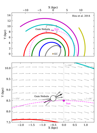
Figure 12: Top panel: Cartoon showing the location of the Gum Nebula in the disk of the Milky Way. The coloured lines trace the polynomial-logarithmic spiral arm models of Hou & Han (2014). A dashed magenta line plots the solar circle at a Galactic radius of 8.5 kpc. Bottom panel: Illustration of the fitted magnetic field orientation around the Gum Nebula. The plot covers the region inside the grey box in the upper panel and the Gum nebula is shown by a black circle (to scale). The three thick arrows piercing the Gum Nebula show the median (black) and $\pm$1-sigma ranges (grey) of field orientation found by fitting the RMs in $\S\ref{sec:results_fit}$. The field of thin grey vectors depicts the orientation of a spiral magnetic field with a pitch-angle of $\wp=-7.2\mbox{${}^{\circ}$}$.

When viewed face-on to the Galactic disk, the direction of the large-scale Galactic magnetic field is characterised by the pitch angle, defined as the deviation from a circular path around the Galactic centre and given by $\wp={\rm tan}^{-1}(B_{\rm rad}/B_{\rm az})$, where $B_{\rm radial}$ and $B_{\rm az}$ are the radial and azimuthal components of the ordered field, respectively. In external spiral galaxies the magnetic field lines are observed to closely follow the spiral arm pattern, but the field strength is often greatest in the inter-arm region (see the examples of Beck et al. 2005, Fletcher et al. 2004 and Patrikeev et al. 2006). In the Milky Way, the ordered disk field is directed parallel to the disk with a typical strength of $B_{0}=1.5\,-\,2\,\mu{\rm G}$ (Han et al. 2006). The pitch angle of the field in the disk has been estimated by multiple authors using a variety of techniques and has been found to lie between $-6\mbox{${}^{\circ}$}$ and $-11.5\mbox{${}^{\circ}$}$, depending on the method used and the volume of the Galaxy observed. There is also some evidence that $\wp$ may have a radial dependence, decreasing to almost zero at galactocentric radii greater than the solar orbit (Van Eck et al. 2011; Jansson & Farrar 2012). Table 3 summarises the results of individual studies in the literature.

The pitch angle $\wp$, Galactic longitude $l$ and fitted magnetic field angle $\Theta$ are related by simple geometry via $l-180\mbox{${}^{\circ}$}=\Theta+\wp$. At the Galactic longitude of the Gum nebula ($l\approx 258.0\mbox{${}^{\circ}$}$) the median pitch angle of $\wp\approx-7.2\mbox{${}^{\circ}$}$ from Table 3 implies an ordered field pointing almost directly towards the observer ($\Theta=85.2\mbox{${}^{\circ}$}$). Our best-fitting shell models presented in $\S\ref{sec:results_fit}$ return field directions between $+43\mbox{${}^{\circ}$}\lesssim\Theta\lesssim+55\mbox{${}^{\circ}$}$, equivalent to a pitch angle range $+23\mbox{${}^{\circ}$}\lesssim\wp\lesssim+35\mbox{${}^{\circ}$}$, substantially different to previous results from the literature. Taking the $\pm 1\sigma$ limits for all models, the local pitch angle is constrained by our data to $+7\mbox{${}^{\circ}$}\lesssim p\lesssim+44\mbox{${}^{\circ}$}$. This range represents the pitch angle of the uniform ambient field local to the Gum Nebula. Our results are illustrated in Fig. 12, which shows the position of the Gum Nebula with respect to the Galactic spiral arms (Hou & Han 2014) and an ideal uniform field with $\wp=-7.2\mbox{${}^{\circ}$}$. All of the investigations referenced in Table 3 calculated the ‘global’ pitch angle averaged along the line-of-sight to pulsars, radio-galaxies or stars. All but one study (Pavel et al. 2012) covered a broad swathe in Galactic longitude. As such, the derived pitch angle is an average over a large fraction of the Galactic disk. By contrast, the method presented here probes only the magnetic field around the Gum Nebula, on scales of $\sim 260$ pc (the diameter of the nebula).

Only a handful of other studies have used bubbles as probes of Galactic magnetic field structure: Kothes & Brown (2009) studied two SNR in the Canadian Galactic Plane Survey (Taylor et al. 2003) and found support for an azimuthal disk field, while Ransom et al. (2010) performed a similar study using old planetary nebulae, but derived only the line-of-sight field strength. Most recently Whiting et al. (2009) and Savage et al. (2013) derived the angle of the magnetic field by modelling H II region shells and found field directions compatible with the mean Galactic field.

We caution that some of the deviation in $\wp$ may be due to systematic errors in the data. As discussed in $\S\ref{sec:model_limitations}$, $\Theta$ is sensitive to longitudinal gradients in RM introduced by contaminating magneto-ionic material, or by the Galaxy in the background. We have taken all reasonable steps to identify and eliminate such contamination, however, a definitive correction requires much more finely sampled and accurate grid of RMs.

Table 3: Studies of ordered magnetic field pitch angle in the literature.

Pitch Angle	Reference	Notes
$+16\mbox{${}^{\circ}$}\pm 4\mbox{${}^{\circ}$}$	Inoue & Tabara (1981)	Radio-galaxies, $<2$ kpc, Orion arm
$-6\mbox{${}^{\circ}$}$	Vallee (1988)	Pulsars, few kpc, Sagittarius and Perseus arms
$-8.2\mbox{${}^{\circ}$}\pm 0.5\mbox{${}^{\circ}$}$	Han & Qiao (1994)	Pulsars (thin disk) and radio-galaxies (thick disk) $\sim 3$ kpc
$-8\mbox{${}^{\circ}$}$	Han et al. (1999)	Pulsar RMs, $\sim 15$ kpc
$-7.2\mbox{${}^{\circ}$}\pm 4.1\mbox{${}^{\circ}$}$	Heiles (1996)	Starlight polarisation, few kpc
$-11.5\mbox{${}^{\circ}$}$	Van Eck et al. (2011)	Radio-galaxies, Galactic sector average
$-6\mbox{${}^{\circ}$}\pm 2\mbox{${}^{\circ}$}$	Pavel et al. (2012)	Radio-galaxies, average along $l=150\mbox{${}^{\circ}$}$

The best fitting ambient magnetic field strength of $B_{0}=3.9^{+4.9}_{-2.2}\,\mbox{$\mu$G}$ is within the range of $2\,\mbox{$\mu$G}$ to $15\,\mbox{$\mu$G}$ observed by similar studies of H II regions (Gaensler et al. 2001; Harvey-Smith et al. 2011). As shown in Fig. 10, $B_{0}$ is correlated with $f$, which is very poorly constrained by the data. The value of $B_{0}$ above is reported for $f=0.3$, the mean of the marginalised likelihood distribution. If instead $f$ is set to the most likely value of $f=0.24$ then $B_{0}\approx 5\,\mbox{$\mu$G}$. The strength of the field within the shell depends on the position, and varies between the ambient level and a maximum value of $X\,\times B_{0}\approx 23\,\mbox{$\mu$G}$ when the $\overrightarrow{B_{0}}$ lies parallel to the edge of the nebula.

In summary, the pitch angle of the ordered magnetic field threading the Gum Nebula ($7\mbox{${}^{\circ}$}\lesssim\wp\lesssim 44\mbox{${}^{\circ}$}$) is significantly different to previous measurements, most of which were averaged over kiloparsec-sized volumes. Few small scale measurements of the field in the diffuse ionised medium exist, so this result may represent typical deviations on scales of a few hundred parsecs. Indeed, Frisch et al. (2012) measured even larger deviations in the ordered magnetic field in the vicinity of the Sun ($<40$ pc), consistent with a scenario where the local ISM is a fragment of the Loop I superbubble. Such deviations have also been observed in external galaxies, for example Heald (2012) detected a significant RM gradient in the spiral galaxy NGC 6946, tracing a irregularity in the vertical component of the ordered magnetic field. The deviation is directly associated with a hole in the H I image and may be ubiquitous feature of star-forming galaxies. Expanding bubbles in the disk may also be responsible for carrying the small-scale turbulent magnetic field into the halo, preventing quenching of the dynamo process and allowing the mean magnetic field to saturate at a strength comparable to equipartition with the turbulent kinetic energy (Shukurov et al. 2006). More accurate and better-sampled RMs are required to confirm our result and eliminate systematic uncertainties. The strength of the ambient field around the Gum Nebula is comparable to average values of $2\,-\,4\,\mbox{$\mu$G}$ measured for the Galaxy as a whole (Han et al. 2006) and within H II regions.

5.3 Implications of the fitted compression factor

The best fitting models presented in $\S\ref{sec:results_fit}$ constrain the jump in density at the edge of the nebula, assuming the shell is 100 percent ionised (by stellar radiation in the case of a H II region or wind-blown-bubble, or by the shock-front in the case of a SNR). The fitted value for the compression factor assuming a flat Galactic background is $X=1.1\,^{+0.5}_{-0.3}$ and assuming a gradient is $X=6.0\,^{+5.1}_{-2.5}$. At the very least, both values imply that the gas within the shell is only moderately compressed compared to the ISM external to the nebula.

The current consensus in the literature is that the nebula is an old supernova remnant (see $\S\ref{sec:gum_history}$). SNR pass through three distinct evolutionary phases (Woltjer 1972) before dissipating: 1) free expansion ($t\lesssim 300$ yr), where the swept-up mass is much less than the ejected mass and the expansion is dominated by the explosion; 2) the Taylor-Sedov phase ($300\,{\rm yr}\lesssim t\lesssim 20000\,{\rm yr}$), where the swept-up mass dominates and the blast wave expands adiabatically and 3) the snow-plough phase ($20000\,{\rm yr}\lesssim t\lesssim 1\,{\rm Myr}$), when thermal cooling has become effective and the shock front decelerates, sweeping up a dense shell. According to the widely used models of Chevalier (1974) the $\sim 260$ pc diameter of the Gum Nebula implies an age of $\sim 1$ Myr, which would be old indeed for an SNR. At this late stage of evolution the shock front is expected to cool radiatively, leading to a compression factor much greater than the values derived here (Cioffi et al. 1988; Cox et al. 1999; Reynolds 2011). Efficient cosmic-ray acceleration processes may also act to increase the compression factor (Vink 2012). At times $t\gtrsim 1$ Myr, SNR expansion is expected to slow down to the ambient sound speed (typically $\sim 10\,\mbox{km\,s${}^{-1}$}$) and merge with the ISM, although the exact details of this process are not clear (Pittard et al. 2003). The expansion velocity measured from optical spectroscopy towards the Gum Nebula is $v\lesssim 10\,\mbox{km\,s${}^{-1}$}$ (Srinivasan et al. 1987, Sahu & Sahu 1993). This slow speed and moderately low compression factor, combined with the flat $n_{e}$ profile derived in $\S\ref{sec:ne}$ make it unlikely that the nebula seen in H $\alpha$ stems solely from a supernova origin. Instead, the detected H $\alpha$ emission and RM-signature are consistent with an ionisation front moving at subsonic speeds into the ISM. Both a classical H II region and wind-blown-bubble are bounded by an ionisation front, so we consider these models in turn below. We cannot completely rule out the old SNR origin as during the dissipation stage the shell likely re-expands, leading to a decrease in density and hence compression factor. However, at this stage, we would also expect the shell to loose cohesion as it merges with the ISM and this is not seen in the H $\alpha$ data towards the Gum Nebula.

The fundamental theory of expanding, over-pressurised H II regions was set out by Strömgren (1939), Kahn (1954) and Oort (1954). After the initial formation phase the H II region expands approximately isothermally (Dyson et al. 1995) until pressure equilibrium is reached. For a high-mass O-type star this does not happen within its stellar lifetime. The D-type ionisation front moves into the ISM at the local sound speed $\lesssim 10\,\mbox{km\,s${}^{-1}$}$ and has a three part structure, consisting of a thin layer of shocked neutral gas separating the unshocked neutral gas from the ionised gas within the H II region. This classical description produces a spherical ionised region of approximately constant electron-density, at odds with the observed shell-like structure of the Gum Nebula seen in H $\alpha$ emission. One possible way to reconcile the model with the data is if the ionisation front is expanding into the walls of a pre-existing cavity. This explanation was first proposed by Reynolds (1976a) whereby the ultraviolet flux from the central stars is ionising the walls of a void and illuminating the ambient magnetic field in the ISM local to the Gum region. Such a cavity could have been formed by an older supernova explosion, or evacuated by an older generation of stars.

The ionised cavity explanation is somewhat contrived, especially since the wind-blown-bubble model can naturally account for the structure and physical parameters of the Gum Nebula measured from observations to date. The star $\zeta$ Puppis is known to drive a powerful stellar wind, as is $\gamma^{2}$ Velorum and the Vela OB2-association (which may also lie inside the Gum Nebula). The Weaver et al. (1977) description of a bubble blown by a high-mass star predicts a shell-like H II region surrounding a region of shocked stellar wind. Indeed, Weaver et al. (1977) offer the Gum Nebula as a prototype wind-blown-bubble powered by the strong stellar winds from $\zeta$ Puppis. Figure 3 in their paper illustrates the temperature and density profile of a typical bubble. The density jump across the outer boundary of the H II shell is $X\approx 1.5$, broadly consistent with our results. In addition, the density in the interior is low at $n_{e}\approx 0.05\,\mbox{cm${}^{-3}$}$ (as is known to be the case for the Gum Nebula) and in the shell is $n_{e}\approx 2.5\,\mbox{cm${}^{-3}$}$, comparable to measurements in this work. Equation 69 in Weaver et al. (1977) describes the density in the shell compared to the ambient upstream density

$$n_{e}=n_{0}\,(V_{2}^{2}+C_{0}^{2})\,/\,C_{s}^{2},$$ (12)

where $V_{2}$ is the shell expansion velocity, $C_{0}$ is the speed of sound in the ISM and $C_{s}$ is the sound speed in the shell. For typical values used in the Weaver et al. (1977) model of the Gum Nebula ($V_{2}\approx 8\,\mbox{km\,s${}^{-1}$}$, $C_{0}\approx 1\,\mbox{km\,s${}^{-1}$}$, $C_{s}\approx 10\,\mbox{km\,s${}^{-1}$}$) then $X=n_{e}/n_{0}=6.5$ in line with our best fitting shell model assuming a background RM-gradient (see $\S\ref{sec:RMs_selected}$).

In summary, we believe our results point to the wind-blown-bubble model as the most likely explanation for the origin of the Gum Nebula.

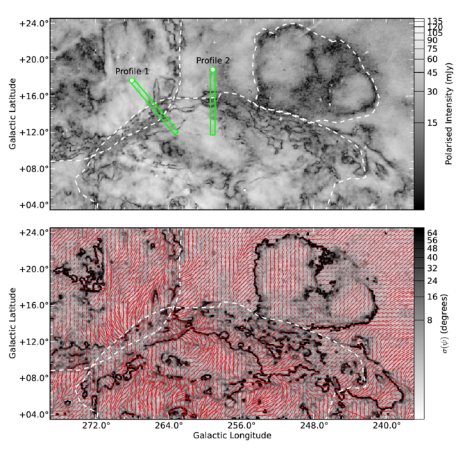
Figure 13: Top panel: Map of the 2.3 GHz polarised intensity for the upper Gum Nebula. Green rectangles show where profiles have been extracted, in Fig. 14 and dotted lines outline the Gum Nebula and Antlia SNR. The profiles run from $(l,b)=(268.0\mbox{${}^{\circ}$},17.7\mbox{${}^{\circ}$})$ to , $(263.1\mbox{${}^{\circ}$},11.9\mbox{${}^{\circ}$})$ and $(259.1\mbox{${}^{\circ}$},18.9\mbox{${}^{\circ}$})$ to $(259.1\mbox{${}^{\circ}$},11.7\mbox{${}^{\circ}$})$ for profiles 1 and 2, respectively. Bottom panel: Map of the dispersion in polarisation angle $\sigma(\psi)$. The value of $\sigma(\psi)$ in each pixel has been calculated from the standard deviation within a beam-sized aperture. Dark canals correspond to regions where the polarisation angle varies by close to $90\mbox{${}^{\circ}$}$ within a beam. The red bars over-plotted on the image every 7th pixel illustrate the orientation of the polarisation vectors (magnetic vector, not corrected for RM).

5.4 Pressure and evolutionary state

The ratio $\beta_{\rm th}=P_{\rm th}/P_{\rm mag}$ of thermal to magnetic pressures in an H II region can indicate whether the object is still evolving or has reached an equilibrium state. In a young H II region, the thermal pressure dominates and drives the expansion of the warm ionised gas into the ISM, sweeping up ambient gas before it. If the region is threaded by a uniform magnetic field, flux-freezing in the ionised gas will resist expansion perpendicular to the field lines. Over time, as the H II region expands, the thermal pressure decreases and the magnetic pressure increases, so ratios closer to unity imply an older object. Magnetic pressure is given by

$$P_{\rm mag}=B_{0}^{2}/\,(8\,\pi)~{}~{}~{}{\rm dyne\,cm^{-2}},$$ (13)

where $B_{0}$ is the total magnetic field strength in $\mu$G. The thermal pressure in an ionised gas at temperature ${\rm T_{e}}$ (in K) and density $n_{e}$ (in cm^-3) is

$$P_{\rm th}=2\,n_{e}\,k\,{\rm T_{e}}~{}~{}~{}{\rm dyne\,cm^{-2}},$$ (14)

where $k$ is Boltzmann’s constant. Assuming ${\rm T_{e}}=8000$ K and $n_{e}=1.4\,\mbox{cm${}^{-3}$}$ for the Gum Nebula, we find $P_{\rm th}=2.9\times 10^{-12}\,{\rm dyne\,cm^{-2}}$ compared to $P_{\rm mag}=6.1\times 10^{-13}\,{\rm dyne\,cm^{-2}}$. The ratio of thermal to magnetic pressure $\beta_{\rm th}=P_{\rm th}/P_{\rm mag}=4.8$ suggests that the dynamics of the shell are dominated by thermal motions, i.e., the magnetic field is too weak to shape the overall morphology of the ionised gas. This result is in keeping with the magneto-hydrodynamic (MHD) simulations of Krumholz et al. (2007) and Arthur et al. (2011), who find that the thermal pressure of the ionised gas shapes the evolution on time-scales of several Myr. Both simulations calculate similar field-strengths and gas-densities to what we derive for the Gum Nebula. Our values for $n_{e}$, $B_{0}$ and $\beta_{\rm th}$ also sit in the middle of the range found by Harvey-Smith et al. (2011) in their survey of high-latitude evolved H II regions.

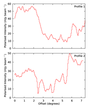
Figure 14: Two profiles extracted from the map of the 2.3 GHz polarised intensity. The tracks along which the profiles have been extracted are illustrated by the green boxes in Fig. 13 and the starting positions marked by circles.

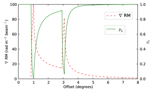
Figure 15: The depolarising effect of the spatial gradient in RM at the inner and outer edge of an ionised shell. The dotted/red line shows the gradient in rotation measure ($d{\rm RM}/dr$) in units of $\mbox{rad\,m${}^{-2}$}\,{\rm beam}^{-1}$ as a function of position, crossing the shell from outside to the interior. The solid/green line shows the corresponding degree of polarisation calculated from Equation 17.

5.5 Radio Spectral Index

The Gum Nebula is a prominent foreground feature in the recently released Planck all-sky radio-continuum maps (Planck Collaboration et al. 2014a). The $\sim 36\mbox{${}^{\circ}$}$ angular diameter shell is visible in the 28.4 GHz image at the $\sim 10\sigma$ level and in the 44.1 GHz image at the $\sim 3\sigma$ level, implying a flat spectral index and a significant thermal component to the emission. A more quantative method of determining the spectral index of diffuse emission is provided by the temperature-temperature (TT) plot (e.g., Tian & Leahy 2006). An x-y plot of the flux densities within a sampling aperture results in a scatter plot and the slope of a straight line fit to the data gives the spectral index $S=S_{0}\nu^{\alpha}$. The main advantage of a TT-plot is that large scale offsets in the background emission are automatically compensated for, assuming that the background does not vary significantly within the sampling box. We find that the spectral index of the Gum Nebula shell at the brightest region is $\alpha=0.2\pm 0.2$, based on a comparison of the 28.4 GHz Planck data and 2.3 GHz S-PASS data; consistent with thermal free-free radio emission. We note that parts of the Gum Nebula are also faintly visible in the 408 MHz radio-continuum map of Haslam et al. (1982), implying a mixture of thermal and synchrotron emission in places.

Further investigation of the spectral index throughout the Gum Nebula is beyond the scope of this work and should be the subject of a separate paper. There now exist many wide-angle maps of radio-continuum emission covering the Gum Nebula, including historical data (e.g., 45 MHz: Maeda et al. 1999, 1.4 GHz: Reich et al. 2001 and Calabretta et al. 2014, 300 MHz - 1.8 GHz: Wolleben et al. 2009, 5 GHz: King et al. 2010, 23 - 94 GHz: Bennett et al. 2013) and new diffuse polarisation maps from Planck and the Murchison Widefield Array (Tingay et al. 2013). Future investigations combining these datasets will be capable of disentangling emission due to synchrotron, free-free and ‘spinning dust’ processes across the region.

5.6 Polarised 2.3 GHz radio-continuum emission

The properties of the diffuse polarised 2.3 GHz radio emission provide complementary information to the RMs of background radio-galaxies. In particular, analysis of the polarised intensity and the angle of the linear polarisation vector can yield information on the geometry and the level of turbulence in the ionised gas.

Fig. 13 presents two views of the polarised 2.3 GHz emission centred on the upper shell of the Gum Nebula. The top panel displays a high resolution image of the polarised intensity ($P=\sqrt{U^{2}+Q^{2}}$). The rim of the Gum Nebula stands out as a broad ($\sim 2\mbox{${}^{\circ}$}$ wide) band of depolarisation across the centre of the image. In addition to the Gum Nebula, two other objects have been identified in the field. The edge of the Antlia SNR $\S\ref{sec:RMs_selected}$, (McCullough et al. 2002) is visible in the upper-left quadrant as an arc of weaker depolarisation and narrow canal-like features. Such canals trace regions where the polarisation angle $\psi$ varies significantly across a telescope beam, leading to depolarisation in the receiver (Fletcher & Shukurov 2006). The Antlia SNR overlaps the Gum Nebula between $163\mbox{${}^{\circ}$}<l<172\mbox{${}^{\circ}$}$, where the H $\alpha$ emission is brightest (see Fig. 1). Also visible are prominent depolarisation canals from a pair of shells in the upper-right quadrant of the image (see $\S\ref{sec:RMs_selected}$). Iacobelli et al. (2014) have analysed the spatial polarisation gradient (Gaensler et al. 2011) in the S-PASS data and have identified these features as the signature of weak shocks (see Burkhart et al. 2012). It is not known if either object is physically interacting with the Gum Nebula, or is simply seen in projection along the line-of-sight. The bottom panel plots the polarisation angle of the electric vector (red bars) over an image of the spatial dispersion in the polarisation angle ( $\sigma(\psi)={\rm stdev}(\psi)$, Hildebrand et al. 2009). Maps of $\sigma(\psi)$ have been shown to highlight depolarisation canals (Planck Collaboration et al. 2014b) and are useful way of visualising where the polarisation vectors are homogeneous or heterogeneous on the sky. Within the Gum Nebula and Antlia SNR the polarised intensity is patchy and the polarisation angles are chaotic in comparison to the slowly varying distribution of angles outside their borders. We interpret this as a ‘scrambling’ of the smooth synchrotron emission from the Galaxy in the background by Faraday screens associated with each object (e.g., Carretti et al. 2013b). It is clear from previous studies (e.g., Duncan et al. 1996) and radio-continuum data (see $\S\ref{sec:SI}$) that emission from the Gum Nebula is dominated by thermal processes. The shell of the nebula does not emit significant amounts of synchrotron radiation and so can be analysed as a pure Faraday screen. Assuming a smooth synchrotron background of polarised synchrotron radiation from the Galaxy, we can quantify the effects of the screen by examining how the level of polarisation changes across the edge of the Gum Nebula.

Fig. 14 presents two polarised profiles extracted from the polarised intensity map. Profile 1 cuts across the brightest region of shell, where it overlaps the weaker Antlia SNR and Profile 2 has been extracted from the upper part of the shell. Profile 1 drops from a high of $\sim 55\,\mbox{mJy\,beam${}^{-1}$}$ outside the shell to a low of $15\,\mbox{mJy\,beam${}^{-1}$}$ inside the depolarised region. The typical root-mean-squared intensity in the $P$ image is $2.2\,{\rm m}\mbox{Jy\,beam${}^{-1}$}$ and the broad depolarisation band exhibits polarised emission at a $\sim 5\sigma$ level. Assuming the outer value represents the intrinsic polarised intensity $P_{i}$, then the degree of depolarisation implied by the drop to $P_{0}=15\,\mbox{mJy\,beam${}^{-1}$}$ is $p=P_{o}/P_{i}\approx 0.27$. The drop in intensity and degree of depolarisation is similar for Profile 2.

5.6.1 Depolarisation

The causes of depolarisation have been described in detail by Burn (1966), Tribble (1991) and Sokoloff et al. (1998). The root cause in all cases is cancellation between polarisation vectors over some averaging interval in time, space or frequency.

Bandwidth depolarisation occurs when Faraday rotation causes the polarisation angle to vary across a frequency averaging window $\Delta\nu$. The degree of depolarisation due to frequency averaging is

$$p=\left|\frac{\rm sin\,\Delta\psi}{\Delta\psi}\right|,$$ (15)

where the change in angle across a band centred on $\nu_{0}$ is given by $\Delta\psi=-2\,{\rm RM}\,c^{2}\,\Delta\nu\,/\,\nu_{0}^{3}$. In the Gum Nebula the maximum RM detected is $\sim 350\,\mbox{rad\,m${}^{-2}$}$ so the expected angle change over the 244 MHz bandwidth is $\Delta\psi=72\mbox{${}^{\circ}$}$ and the resultant depolarisation is negligible at $p=0.75$. A RM of $870\,\mbox{rad\,m${}^{-2}$}$ would be necessary to completely depolarise S-PASS data.

The most likely depolarisation mechanism affecting the S-PASS data is beam depolarisation. This is caused by variations in $B_{||}$ or $n_{e}$ on scales much smaller than the beam, scattering the polarisation angles on adjacent lines of sight. Burn (1966) quantified this effect in the simplest case of a uniform slab and found

$$p={\rm exp}\,(-2\,\sigma_{\rm RM}^{2}\,\lambda^{4}),$$ (16)

where $\sigma_{\rm RM}$ is the RM scatter within a beam after measurement errors have been accounted for. If small-scale random fluctuations are solely responsible for the observed depolarisation ($p=0.27$) then Equation 16 predicts an excess scatter of $\sigma_{\rm RM}=47\,\mbox{rad\,m${}^{-2}$}$. In $\S\ref{sec:results_fit}$ we found that the best-fitting model implied an additional scatter of $\sigma_{\rm RM}=78.6\,\mbox{rad\,m${}^{-2}$}$ (called $\delta({\rm RM})$ in Table 2). This fitted value is an upper-limit on $\sigma_{\rm RM}$ as the RM sampling grid is very coarse at ${\rm\sim 1/degree^{2}}$, compared to the beam FWHM of $\Theta_{\rm beam}=10.75^{\prime}$. We can conclude that the data is at least consistent with a large fraction of the depolarisation being due to random fluctuations in $B_{||}$ or $n_{e}$.

While the average drop in $P$ can be explained (at least in part) by fluctuations within an ionised Faraday screen, the shell of the nebula also contains depolarisation canals. These are typically one beam in width, close to 100 percent depolarised and tend to be aligned parallel to the edge of the nebula. First discovered by Haverkorn et al. (2000), several authors in the last decade have studied origin of such canals and explored their use as a diagnostic tool (e.g., Fletcher & Shukurov 2006, Gaensler et al. 2011 and Burkhart et al. 2012). In particular, Gaensler et al. (2011) calculated the spatial gradient of the complex Stokes vector $\overrightarrow{P}=(\overrightarrow{Q},\,\overrightarrow{U})$, whose magnitude $|\nabla\,P|$ describes the rate at which the polarisation vector traces out a path in the $Q$ – $U$ plane when moving along a spatial track at a constant rate. $|\nabla\,P|$ is invariant under arbitrary rotations or translations (unlike $P$ or $\psi$) and images of $|\nabla\,P|$ reveal a network of filaments in the ionised gas (see Iacobelli et al. 2014 for the $|\nabla\,P|$ of the S-PASS data). In a pure Faraday screen these filaments have been shown to trace spatial cusps or jumps in $n_{e}$ or $B_{||}$, most likely caused by shock-fronts or turbulent motions in the gas (Burkhart et al. 2012). Depolarisation canals like those in Figure 13 are a subset of filaments that cross the origin in the $Q$ – $U$ plane. The greatest concentration of canals occur within the rim of the nebula, lending weight to our conclusion that turbulent fluctuations in $n_{e}$ or $B_{||}$ are responsible for the depolarisation.

The most prominent canals run along the inner and outer edges of the depolarised rim and can be explained by the intrinsic RM-gradient at the edges of the ionised shell. The amount of depolarisation produced by an RM-gradient is given by Sokoloff et al. (1998) as

$$p_{g}=exp\,\left[-\frac{1}{ln\,2}\,\left(\frac{d{\rm RM}}{dr}\right)^{2}\,\lambda^{4}\,\right],$$ (17)

assuming a Gaussian beam which resolves the gradient. Fig. 15 plots the RM-gradient and the depolarisation factor calculated from the Equation 17 for a profile crossing towards the interior of the ionised shell. From the plot we see that depolarisation only becomes significant ($p<0.6$) close to peaks in the gradient. The equation breaks down for resolved gradients, however, it is clear that narrow depolarisation canals are predicted at the leading and inner edges of the shell.

In conclusion, the polarisation and depolarisation properties of the 2.3 GHz S-PASS data are in keeping with the simple ionised shell model put forward in $\S\ref{sec:mag_bubble}$ and support our assertion that the Gum Nebula is acting as a Faraday screen.

5.7 Comparison to previous studies

The first dedicated magnetic field measurements of the Gum Nebula were obtained by Vallee & Bignell (1983) via linear polarisation observations of 35 background extragalactic radio sources. Prior to that work, large-scale rotation measure excesses in the area were attributed to a tangential view of the local Orion-spur spiral arm (Simard-Normandin & Kronberg 1980). Vallee & Bignell (1983) claimed that the distribution of RMs on the sky were not consistent with the arm model but were a good match for the old SNR model first presented by Reynolds (1976b). Their derived line-of-sight magnetic field strength of $\sim 1.3\,\mu$G suggested that a ‘snow-plough’ effect alone was responsible for sweeping up gas, and hence the magnetic field lines. In later work, Duncan et al. (1996) cast doubt on the significance of the Vallee model, pointing out that the statistical uncertainty in the data used therein was comparable to the mean RM value. The model presented in this paper is broadly consistent with the Vallee & Bignell (1983) result, but is considerably more sophisticated and includes much better sampled measurements of RM and $n_{e}$. We also derive independent values for the shell thickness and compression factor, which Vallee & Bignell (1983) did not provide.

Magnetic field strengths in ionised bubbles have been measured by a number of recent studies in the literature. Whiting et al. (2009) and Savage et al. (2013) used a similar technique to the one presented here to study the bubble surrounding the Cygnus OB1 association and the Rosette nebula, respectively. Whiting et al. (2009) suggested that the observed Faraday ‘anomaly’ was caused by a wind-blown bubble, but with only nine RMs they could not confirm the compression factor predicted by the strong shock. On the other hand, Savage et al. (2013) modelled RMs seen through the Rosette nebula as a limb-brightened ionised shell and obtained a considerably better fit when fixing $X=4$ compared to $X=1$. Recently, Harvey-Smith et al. (2011) studied the line of sight magnetic fields in five large-diameter H II regions offset from the Galactic plane. They derived field strengths from $\sim 3\,-\,11\,\mu$G, but found no evidence of compression at the edges of these relatively evolved H II regions.

6 Summary and Conclusions

We have developed a simple model of the Gum Nebula as an expanding ionised shell threaded by a uniform magnetic field. Drawing upon the RM catalogue of Taylor et al. (2009) and the H $\alpha$ image of Finkbeiner (2003), we used a maximum-likelihood MCMC analysis to derive the magneto-ionic shell parameters in the upper hemisphere of the nebula. We compared the best-fitting models to polarised 2.3 GHz radio-continuum emission from the S-PASS project. Our conclusions are as follows:

1. The RM and EM data covering the upper hemisphere of the Gum Nebula ($b>5\mbox{${}^{\circ}$}$) are well-fitted by a simple ionised shell. Assuming a large-scale RM-background from the Sun et al. (2008) model of the Galaxy, the best-fitting shell has an angular radius $\phi_{\rm outer}=22.7\mbox{${}^{\circ}$}^{+0.1}_{-0.1}$, shell thickness $dr=18.5^{+1.5}_{-1.4}\,{\rm pc}$, ambient magnetic field strength $B_{0}=3.9^{+4.9}_{-2.2}\,\mbox{$\mu$G}$, electron density $n_{e}=1.4^{+0.4}_{-0.4}\,{\rm cm^{-3}}$ and filling factor $f=0.3^{+0.3}_{-0.1}$

2. We constrain the pitch angle of the uniform magnetic field to values over the range $+7\mbox{${}^{\circ}$}\lesssim\wp\lesssim+44\mbox{${}^{\circ}$}$, significantly different from previously derived values ($\wp\approx-7\mbox{${}^{\circ}$}$) averaged over much larger volumes of the Galactic disk (scales of several kpc versus $\sim 260$ pc for the Gum Nebula). Our fitted values are sensitive to contamination of the RMs by intervening magneto-ionic objects, however, we have corrected the catalogues to the full extent allowed by the available data. This represents one of the few measurements of local magnetic field orientation in the Milky Way.

3. We find that the compression factor $X=n_{e}/n_{0}$ at the edge of the H $\alpha$ shell is $X=6.0\,^{+5.1}_{-2.5}$, assuming an RM-background from Sun et al. (2008). This value is much lower than expected if the Gum Nebula were an old SNR cooling radiatively. We believe that the most likely explanation for the nebula is a wind-blown-bubble driven by a cluster of high-mass stars. The slow expansion velocity ($\lesssim 10\,\mbox{km\,s${}^{-1}$}$), low excitation conditions and lack of radio-synchrotron emission from the rim is consistent with our hypothesis.

4. The strength of the ordered magnetic field $B_{0}$ is not well measured as it is degenerate with the ill-constrained filling factor $f$. We derive a value of $B_{0}=3.9^{+4.9}_{-2.2}\,\mbox{$\mu$G}$, in line with the strength of the ambient Galactic field and also comparable with values measured towards H II regions by previous authors.

5. Viewed in 2.3 GHz radio-continuum, the upper shell of the Gum Nebula exhibits a distinctive band of depolarised emission. We find that the dominant depolarising mechanism is likely due to fluctuations in $n_{e}$ and the random component of $\overrightarrow{B}_{o}$ on scales much smaller than the $10.75^{\prime}$ beam. The depolarised canal features observed at the boundary of the band are consistent with being caused by RM-gradients at the edge of the ionised shell.

The study presented here illustrates how even large objects, well-sampled by RMs, require great care to disentangle from confusing sources. The next generation of surveys planned for the Square Kilometer Array and precursors instruments will enable similar studies of many more Galactic objects. From 2016 onwards the Australia Square Kilometre Array Pathfinder (ASKAP, Johnston et al. 2007) POSSUM (Polarisation Sky Survey of the Universe’s Magnetism) project (Gaensler et al. 2010) will survey the southern sky at 1 GHz and deliver a RM-grid with $\sim$100 polarised sources per square degree ($\sim 100$ times the source density of the NVSS). Once the new catalogue becomes available it will be possible to identify and correct for smaller Faraday-active objects with greater accuracy and confidence. This work serves as a rehersal for future studies and highlights the challenges involved.

Appendix A Geometry of Simple Ionised Shell Model

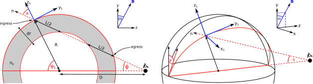
Figure 16: Geometry of an ionised shell in the near-field. We assume a constant electron density $n_{e}$ in the shell, which is threaded with a uniform magnetic field. The field is confined to the y-z plane, representing the Galactic disk, and only the sky pitch-angle $\Theta$ may be varied.

The geometry of our simple shell model is shown schematically in Fig. 16. It consists of a spherical ionised region of radius $R$ and thickness $dr$, containing thermal electrons at an average density $n_{e}$. The edge of the shell subtends an angular radius $\phi_{\rm outer}={\rm sin}^{-1}(R/D)$, where $D$ is the distance from the observer to the geometric centre. The ionised gas is threaded by a uniform magnetic field $\overrightarrow{B_{0}}$, whose vector is confined to the y-z plane representing the Galactic disk. Field lines make an angle $\Theta$ to the plane of the sky in the direction of the bubble centre. From the perspective of an external observer, the angle $\zeta$ describes the orientation of the sight-line to the y-z plane. The observed RM is given by Equation 3 and in the simplest case ($\zeta=0$, Fig. 16 - left) depends only on the line-of-sight field strength $B_{||}$ and the path-length L along a chord through the shell:

$$B_{||}=-B_{0}\,{\rm sin}(\Theta-\phi),$$ (A1)

$$L(\phi)=2\,\sqrt{D^{2}\left[{\rm sin}^{2}(\phi_{\rm outer})-{\rm sin}^{2}(\phi)\right]}.$$ (A2)

If the shell is compressing the ionised gas at the leading edge then the components of $\overrightarrow{B_{0}}$ tangent to the surface will be amplified by a factor $X$. To model this effect we decompose $\overrightarrow{B_{0}}$ at each point on the surface into vector components ($B_{x_{1}}$, $B_{y_{1}}$, $B_{z_{1}}$) along the axes $x_{1}$, $y_{1}$ and $z_{1}$ such that

$$B_{x_{1}} =B_{0}~{}{\rm cos}(\Theta)\,{\rm sin}(\zeta),$$ (A3)

$$B_{y_{1}} =B_{0}~{}\left[~{}{\rm cos}(\Theta)\,{\rm cos}(\zeta)\,{\rm cos}(\phi_{1})+{\rm sin}(\Theta)\,{\rm sin}(\phi_{1})~{}\right],$$ (A4)

$$B_{z_{1}} =B_{0}~{}\left[~{}{\rm cos}(\Theta)\,{\rm cos}(\zeta)\,{\rm sin}(\phi_{1})-{\rm sin}(\Theta)\,{\rm cos}(\phi_{1})~{}\right].$$ (A5)

The observed magnetic field strength is then the vector sum along the line-of-sight at both the ingress ($B_{i}$) and egress ($B_{e}$) points. From the geometry we find

$$B_{i} =X\,B_{y_{1}}~{}{\rm sin}(a)-B_{z_{1}}~{}{\rm cos}(a),$$ (A6)

$$B_{e} =X\,B_{y_{1}}~{}{\rm sin}(a)+B_{z_{1}}~{}{\rm cos}(a),$$ (A7)

where $a={\rm sin}^{-1}(\phi/\phi_{\rm outer})$. When calculating $B_{i}$ the angle $\phi_{1}$ in Equations A3 - A5 is sampled over the far side of the sphere according to $\phi_{1}=a+\phi$. Similarly, when calculating $B_{e}$, $\phi_{1}$ is sampled over the near side: $\phi_{1}=180\mbox{${}^{\circ}$}-a+\phi$. The final line-of-sight magnetic field strength is then given by

$$B_{||}=(B_{i}+B_{e})\,/\,2,$$ (A8)

assuming $B_{i}$ and $B_{e}$ are constant along the path connecting the midpoint of the chord and the surface of the shell. The RM at any point may then be calculated by combining Equations A2 - A8 with Equation 4.

References

- Alexander et al. (1971) Alexander, J. K., Brandt, J. C., Maran, S. P., & Stecher, T. P. 1971, ApJ, 167, 487
- Arthur et al. (2011) Arthur, S. J., Henney, W. J., Mellema, G., de Colle, F., & Vázquez-Semadeni, E. 2011, MNRAS, 414, 1747
- Astropy Collaboration et al. (2013) Astropy Collaboration, Robitaille, T. P., Tollerud, E. J., et al. 2013, A&A, 558, A33
- Beck et al. (2005) Beck, R., Fletcher, A., Shukurov, A., et al. 2005, A&A, 444, 739
- Bennett et al. (2013) Bennett, C. L., Larson, D., Weiland, J. L., et al. 2013, ApJS, 208, 20
- Beuermann (1973) Beuermann, K. P. 1973, Ap&SS, 20, 27
- Bisscheroux et al. (1997) Bisscheroux, B. C., Pols, O. R., Kahabka, P., Belloni, T., & van den Heuvel, E. P. J. 1997, A&A, 317, 815
- Brandt et al. (1971) Brandt, J. C., Stecher, T. P., Crawford, D. L., & Maran, S. P. 1971, ApJ, 163, L99
- Burkhart et al. (2012) Burkhart, B., Lazarian, A., & Gaensler, B. M. 2012, ApJ, 749, 145
- Burn (1966) Burn, B. J. 1966, MNRAS, 133, 67
- Calabretta et al. (2014) Calabretta, M. R., Staveley-Smith, L., & Barnes, D. G. 2014, PASA, 31, 7
- Carretti (2011) Carretti, E. 2011, Journal of Astrophysics and Astronomy, 32, 457
- Carretti et al. (2004) Carretti, E., Cortiglioni, S., Sbarra, C., & Tascone, R. 2004, A&A, 420, 437
- Carretti et al. (2010) Carretti, E., Haverkorn, M., McConnell, D., et al. 2010, MNRAS, 405, 1670
- Carretti et al. (2013a) Carretti, E., Brown, S., Staveley-Smith, L., et al. 2013a, MNRAS, 430, 1414
- Carretti et al. (2013b) Carretti, E., Crocker, R. M., Staveley-Smith, L., et al. 2013b, Nature, 493, 66
- Chanot & Sivan (1983) Chanot, A., & Sivan, J. P. 1983, A&A, 121, 19
- Chevalier (1974) Chevalier, R. A. 1974, ApJ, 188, 501
- Choudhury & Bhatt (2009) Choudhury, R., & Bhatt, H. C. 2009, MNRAS, 393, 959
- Churchwell et al. (1996) Churchwell, E., Winnberg, A., Cardelli, J., Cooper, G., & Suntzeff, N. B. 1996, ApJ, 469, 209
- Churchwell et al. (2006) Churchwell, E., Povich, M. S., Allen, D., et al. 2006, ApJ, 649, 759
- Cioffi et al. (1988) Cioffi, D. F., McKee, C. F., & Bertschinger, E. 1988, ApJ, 334, 252
- Condon et al. (1996) Condon, J. J., Cotton, W. D., Greisen, E. W., et al. 1996, Astronomy Data Image Library, 1
- Cordes & Lazio (2002) Cordes, J. M., & Lazio, T. J. W. 2002, arXiv: astro-ph/0207156
- Cox et al. (1999) Cox, D. P., Shelton, R. L., Maciejewski, W., et al. 1999, ApJ, 524, 179
- De Marco & Schmutz (1999) De Marco, O., & Schmutz, W. 1999, A&A, 345, 163
- de Zeeuw et al. (1999) de Zeeuw, P. T., Hoogerwerf, R., de Bruijne, J. H. J., Brown, A. G. A., & Blaauw, A. 1999, AJ, 117, 354
- Dennison et al. (1998) Dennison, B., Simonetti, J. H., & Topasna, G. A. 1998, PASA, 15, 147
- Dodson et al. (2003) Dodson, R., Legge, D., Reynolds, J. E., & McCulloch, P. M. 2003, ApJ, 596, 1137
- Dove et al. (2000) Dove, J. B., Shull, J. M., & Ferrara, A. 2000, ApJ, 531, 846
- Draine (2011) Draine, B. T. 2011, Physics of the Interstellar and Intergalactic Medium by Bruce T. Draine. Princeton University Press, 2011. ISBN: 978-0-691-12214-4
- Drimmel & Spergel (2001) Drimmel, R., & Spergel, D. N. 2001, ApJ, 556, 181
- Dubner et al. (1992) Dubner, G., Giacani, E., Cappa de Nicolau, C., & Reynoso, E. 1992, A&AS, 96, 505
- Duncan et al. (1996) Duncan, A. R., Stewart, R. T., Haynes, R. F., & Jones, K. L. 1996, MNRAS, 280, 252
- Dyson et al. (1995) Dyson, J. E., Williams, R. J. R., & Redman, M. P. 1995, MNRAS, 277, 700
- Finkbeiner (2003) Finkbeiner, D. P. 2003, ApJS, 146, 407
- Fletcher et al. (2004) Fletcher, A., Berkhuijsen, E. M., Beck, R., & Shukurov, A. 2004, A&A, 414, 53
- Fletcher & Shukurov (2006) Fletcher, A., & Shukurov, A. 2006, MNRAS, 371, L21
- Foreman-Mackey et al. (2013) Foreman-Mackey, D., Hogg, D. W., Lang, D., & Goodman, J. 2013, PASP, 125, 306
- Frisch et al. (2012) Frisch, P. C., Andersson, B.-G., Berdyugin, A., et al. 2012, ApJ, 760, 106
- Gaensler et al. (2001) Gaensler, B. M., Dickey, J. M., McClure-Griffiths, N. M., et al. 2001, ApJ, 549, 959
- Gaensler et al. (2010) Gaensler, B. M., Landecker, T. L., Taylor, A. R., & POSSUM Collaboration. 2010, in BAAS, Vol. 42, AAS Meeting Abstracts 215, Page. 470.13
- Gaensler et al. (2008) Gaensler, B. M., Madsen, G. J., Chatterjee, S., & Mao, S. A. 2008, PASA, 25, 184
- Gaensler et al. (2011) Gaensler, B. M., Haverkorn, M., Burkhart, B., et al. 2011, Nature, 478, 214
- Gaustad et al. (2001) Gaustad, J. E., McCullough, P. R., Rosing, W., & Van Buren, D. 2001, PASP, 113, 1326
- Goodman & Were (2010) Goodman, J., & Were, J. 2010, Communications in Applied Mathematical and Computational Science, 5, 65
- Gum (1952) Gum, C. S. 1952, The Observatory, 72, 151
- Gum (1956) —. 1956, The Observatory, 76, 150
- Haffner et al. (2003) Haffner, L. M., Reynolds, R. J., Tufte, S. L., et al. 2003, ApJS, 149, 405
- Han et al. (2006) Han, J. L., Manchester, R. N., Lyne, A. G., Qiao, G. J., & van Straten, W. 2006, ApJ, 642, 868
- Han et al. (1999) Han, J. L., Manchester, R. N., & Qiao, G. J. 1999, MNRAS, 306, 371
- Han & Qiao (1994) Han, J. L., & Qiao, G. J. 1994, A&A, 288, 759
- Harvey-Smith et al. (2011) Harvey-Smith, L., Madsen, G. J., & Gaensler, B. M. 2011, ApJ, 736, 83
- Haslam et al. (1982) Haslam, C. G. T., Salter, C. J., Stoffel, H., & Wilson, W. E. 1982, A&AS, 47, 1
- Hastings (1970) Hastings, W. 1970, Biometrika, 57, 97
- Haverkorn et al. (2000) Haverkorn, M., Katgert, P., & de Bruyn, A. G. 2000, A&A, 356, L13
- Hawarden & Brand (1976) Hawarden, T. G., & Brand, P. W. J. L. 1976, MNRAS, 175, 19P
- Heald (2012) Heald, G. H. 2012, ApJ, 754, L35
- Heiles (1996) Heiles, C. 1996, ApJ, 462, 316
- Hildebrand et al. (2009) Hildebrand, R. H., Kirby, L., Dotson, J. L., Houde, M., & Vaillancourt, J. E. 2009, ApJ, 696, 567
- Hobson et al. (2002) Hobson, M. P., Bridle, S. L., & Lahav, O. 2002, MNRAS, 335, 377
- Hou & Han (2014) Hou, L. G., & Han, J. L. 2014, ArXiv e-prints
- Iacobelli et al. (2014) Iacobelli, M., Burkhart, B., Haverkorn, M., et al. 2014, A&A, 566, A5
- Inoue & Tabara (1981) Inoue, M., & Tabara, H. 1981, PASJ, 33, 603
- Jackson et al. (2006) Jackson, J. M., Rathborne, J. M., Shah, R. Y., et al. 2006, ApJS, 163, 145
- Jaffe et al. (2010) Jaffe, T. R., Leahy, J. P., Banday, A. J., et al. 2010, MNRAS, 401, 1013
- Jansson & Farrar (2012) Jansson, R., & Farrar, G. R. 2012, ApJ, 757, 14
- Jansson et al. (2009) Jansson, R., Farrar, G. R., Waelkens, A. H., & Enßlin, T. A. 2009, J. Cosmology Astropart. Phys, 7, 21
- Johnston et al. (2007) Johnston, S., Bailes, M., Bartel, N., et al. 2007, PASA, 24, 174
- Kahn (1954) Kahn, F. D. 1954, Bull. Astron. Inst. Netherlands, 12, 187
- King et al. (2010) King, O. G., Copley, C., Davies, R., et al. 2010, in Society of Photo-Optical Instrumentation Engineers (SPIE) Conference Series, Vol. 7741, Society of Photo-Optical Instrumentation Engineers (SPIE) Conference Series, 1
- Kothes & Brown (2009) Kothes, R., & Brown, J.-A. 2009, in IAU Symposium, Vol. 259, Probing interstellar magnetic fields with Supernova remnants, ed. K. G. Strassmeier, A. G. Kosovichev, & J. E. Beckman, 75–80
- Krumholz et al. (2007) Krumholz, M. R., Stone, J. M., & Gardiner, T. A. 2007, ApJ, 671, 518
- Lahav et al. (2000) Lahav, O., Bridle, S. L., Hobson, M. P., Lasenby, A. N., & Sodré, L. 2000, MNRAS, 315, L45
- Lasker (1966) Lasker, B. M. 1966, ApJ, 143, 700
- Leahy et al. (1992) Leahy, D. A., Nousek, J., & Garmire, G. 1992, ApJ, 385, 561
- Maeda et al. (1999) Maeda, K., Alvarez, H., Aparici, J., May, J., & Reich, P. 1999, A&AS, 140, 145
- Manchester et al. (2005) Manchester, R. N., Hobbs, G. B., Teoh, A., & Hobbs, M. 2005, AJ, 129, 1993
- Mao et al. (2010) Mao, S. A., Gaensler, B. M., Haverkorn, M., et al. 2010, ApJ, 714, 1170
- Mathewson & Ford (1970) Mathewson, D. S., & Ford, V. L. 1970, MmRAS, 74, 139
- May et al. (1988) May, J., Murphy, D. C., & Thaddeus, P. 1988, A&AS, 73, 51
- McClure-Griffiths et al. (2009) McClure-Griffiths, N. M., Pisano, D. J., Calabretta, M. R., et al. 2009, ApJS, 181, 398
- McCray & Snow (1979) McCray, R., & Snow, Jr., T. P. 1979, ARA&A, 17, 213
- McCullough et al. (2002) McCullough, P. R., Fields, B. D., & Pavlidou, V. 2002, ApJ, 576, L41
- Metropolis et al. (1953) Metropolis, N., Rosenbluth, A. W., Rosenbluth, M. N., Teller, A. H., & Teller, E. 1953, The Journal of Chemical Physics, 21, 1087
- Mitra & Ramachandran (2001) Mitra, D., & Ramachandran, R. 2001, A&A, 370, 586
- Moss et al. (2012) Moss, V. A., McClure-Griffiths, N. M., Braun, R., Hill, A. S., & Madsen, G. J. 2012, MNRAS, 421, 3159
- Murphy & May (1991) Murphy, D. C., & May, J. 1991, A&A, 247, 202
- O’Dea et al. (2007) O’Dea, D., Challinor, A., & Johnson, B. R. 2007, MNRAS, 376, 1767
- Oey et al. (2005) Oey, M. S., Watson, A. M., Kern, K., & Walth, G. L. 2005, AJ, 129, 393
- Oort (1954) Oort, J. H. 1954, Bull. Astron. Inst. Netherlands, 12, 177
- Oppermann et al. (2012) Oppermann, N., Junklewitz, H., Robbers, G., et al. 2012, A&A, 542, A93
- Patrikeev et al. (2006) Patrikeev, I., Fletcher, A., Stepanov, R., et al. 2006, A&A, 458, 441
- Pavel et al. (2012) Pavel, M. D., Clemens, D. P., & Pinnick, A. F. 2012, ApJ, 749, 71
- Pidopryhora et al. (2007) Pidopryhora, Y., Lockman, F. J., & Shields, J. C. 2007, ApJ, 656, 928
- Pittard et al. (2003) Pittard, J. M., Arthur, S. J., Dyson, J. E., et al. 2003, A&A, 401, 1027
- Planck Collaboration et al. (2014a) Planck Collaboration, Ade, P. A. R., Aghanim, N., et al. 2014a, A&A, 571, A1
- Planck Collaboration et al. (2014b) —. 2014b, arXiv: astroph/1405.0871
- Radhakrishnan & Manchester (1969) Radhakrishnan, V., & Manchester, R. N. 1969, Nature, 222, 228
- Ransom et al. (2010) Ransom, R. R., Kothes, R., Landecker, T. L., & Wolleben, A. M. 2010, in Astronomical Society of the Pacific Conference Series, Vol. 438, Astronomical Society of the Pacific Conference Series, ed. R. Kothes, T. L. Landecker, & A. G. Willis, 268
- Reed (2003) Reed, B. C. 2003, AJ, 125, 2531
- Reich et al. (2001) Reich, P., Testori, J. C., & Reich, W. 2001, A&A, 376, 861
- Reipurth (1983) Reipurth, B. 1983, A&A, 117, 183
- Reynolds (1976a) Reynolds, R. J. 1976a, ApJ, 203, 151
- Reynolds (1976b) —. 1976b, ApJ, 206, 679
- Reynolds (1988) —. 1988, ApJ, 333, 341
- Reynolds et al. (2001) Reynolds, R. J., Sterling, N. C., & Haffner, L. M. 2001, ApJ, 558, L101
- Reynolds (2011) Reynolds, S. P. 2011, Ap&SS, 336, 257
- Reynoso & Dubner (1997) Reynoso, E. M., & Dubner, G. M. 1997, A&AS, 123, 31
- Rodgers et al. (1960) Rodgers, A. W., Campbell, C. T., & Whiteoak, J. B. 1960, MNRAS, 121, 103
- Sahu et al. (1988) Sahu, M., Pottasch, S. R., Sahu, K. C., Wesselius, P. R., & Desai, J. N. 1988, A&A, 195, 269
- Sahu & Sahu (1992) Sahu, M., & Sahu, K. C. 1992, A&A, 259, 265
- Sahu & Sahu (1993) Sahu, M. S., & Sahu, K. C. 1993, A&A, 280, 231
- Sandqvist (1976) Sandqvist, A. 1976, MNRAS, 177, 69P
- Savage et al. (2013) Savage, A. H., Spangler, S. R., & Fischer, P. D. 2013, ApJ, 765, 42
- Schlegel et al. (1998) Schlegel, D. J., Finkbeiner, D. P., & Davis, M. 1998, ApJ, 500, 525
- Shukurov et al. (2006) Shukurov, A., Sokoloff, D., Subramanian, K., & Brandenburg, A. 2006, A&A, 448, L33
- Shull & Draine (1987) Shull, J. M., & Draine, B. T. 1987, in Astrophysics and Space Science Library, Vol. 134, Interstellar Processes, ed. D. J. Hollenbach & H. A. Thronson, Jr., 283–319
- Simard-Normandin & Kronberg (1980) Simard-Normandin, M., & Kronberg, P. P. 1980, ApJ, 242, 74
- Sokoloff et al. (1998) Sokoloff, D. D., Bykov, A. A., Shukurov, A., et al. 1998, MNRAS, 299, 189
- Srinivasan et al. (1987) Srinivasan, M., Pecker, J. C., Pottasch, S. R., & Sahu, K. C. 1987, The Messenger, 50, 11
- Stil & Taylor (2007) Stil, J. M., & Taylor, A. R. 2007, ApJ, 663, L21
- Strömgren (1939) Strömgren, B. 1939, ApJ, 89, 526
- Sun & Reich (2010) Sun, X.-H., & Reich, W. 2010, Research in Astronomy and Astrophysics, 10, 1287
- Sun et al. (2008) Sun, X. H., Reich, W., Waelkens, A., & Enßlin, T. A. 2008, A&A, 477, 573
- Taylor et al. (2009) Taylor, A. R., Stil, J. M., & Sunstrum, C. 2009, ApJ, 702, 1230
- Taylor et al. (2003) Taylor, A. R., Gibson, S. J., Peracaula, M., et al. 2003, AJ, 125, 3145
- Taylor & Cordes (1993) Taylor, J. H., & Cordes, J. M. 1993, ApJ, 411, 674
- Taylor et al. (1993) Taylor, J. H., Manchester, R. N., & Lyne, A. G. 1993, ApJS, 88, 529
- Tian & Leahy (2006) Tian, W. W., & Leahy, D. A. 2006, A&A, 447, 205
- Tingay et al. (2013) Tingay, S. J., Goeke, R., Bowman, J. D., et al. 2013, PASA, 30, 7
- Tribble (1991) Tribble, P. C. 1991, MNRAS, 250, 726
- Tucci et al. (2004) Tucci, M., Martínez-González, E., Toffolatti, L., González-Nuevo, J., & De Zotti, G. 2004, MNRAS, 349, 1267
- Urquhart et al. (2009) Urquhart, J. S., Morgan, L. K., & Thompson, M. A. 2009, A&A, 497, 789
- Vallee (1988) Vallee, J. P. 1988, AJ, 95, 750
- Vallee & Bignell (1983) Vallee, J. P., & Bignell, R. C. 1983, ApJ, 272, 131
- van der Swaluw (2001) van der Swaluw, E. 2001, PhD thesis, Utrecht University
- Van Eck et al. (2011) Van Eck, C. L., Brown, J. C., Stil, J. M., et al. 2011, ApJ, 728, 97
- van Leeuwen (2007) van Leeuwen, F. 2007, A&A, 474, 653
- Vidal (1979) Vidal, J.-L. 1979, A&A, 79, 93
- Vink (2012) Vink, J. 2012, A&A Rev., 20, 49
- Wallerstein et al. (1980) Wallerstein, G., Jenkins, E. B., & Silk, J. 1980, ApJ, 240, 834
- Weaver et al. (1977) Weaver, R., McCray, R., Castor, J., Shapiro, P., & Moore, R. 1977, ApJ, 218, 377
- Whiting et al. (2009) Whiting, C. A., Spangler, S. R., Ingleby, L. D., & Haffner, L. M. 2009, ApJ, 694, 1452
- Woermann et al. (2000) Woermann, B., Gaylard, M. J., & Otrupcek, R. 2000, MNRAS, 315, 241
- Woermann et al. (2001) —. 2001, MNRAS, 325, 1213
- Wolleben et al. (2009) Wolleben, M., Landecker, T. L., Carretti, E., et al. 2009, in IAU Symposium, Vol. 259, IAU Symposium, ed. K. G. Strassmeier, A. G. Kosovichev, & J. E. Beckman, 89–90
- Woltjer (1972) Woltjer, L. 1972, ARA&A, 10, 129
- Zealey (1979) Zealey, W. J. 1979, New Zealand Journal of Science, 22, 549