Asymptotically Exact Error Analysis for the Generalized $\ell_{2}^{2}$-LASSO

Abstract

Given an unknown signal $\mathbf{x}_{0}\in\mathbb{R}^{n}$ and linear noisy measurements $\mathbf{y}=\mathbf{A}\mathbf{x}_{0}+\sigma\mathbf{v}\in\mathbb{R}^{m}$, the generalized $\ell_{2}^{2}$-LASSO solves $\hat{\mathbf{x}}:=\arg\min_{\mathbf{x}}\frac{1}{2}\|\mathbf{y}-\mathbf{A}\mathbf{x}\|_{2}^{2}+\sigma\lambda f(\mathbf{x})$. Here, $f$ is a convex regularization function (e.g. $\ell_{1}$-norm, nuclear-norm) aiming to promote the structure of $\mathbf{x}_{0}$ (e.g. sparse, low-rank), and, $\lambda\geq 0$ is the regularizer parameter. A related optimization problem, though not as popular or well-known, is often referred to as the generalized $\ell_{2}$-LASSO and takes the form $\hat{\mathbf{x}}:=\arg\min_{\mathbf{x}}\|\mathbf{y}-\mathbf{A}\mathbf{x}\|_{2}+\lambda f(\mathbf{x})$, and has been analyzed in [1]. [1] further made conjectures about the performance of the generalized $\ell_{2}^{2}$-LASSO. This paper establishes these conjectures rigorously. We measure performance with the normalized squared error $\mathrm{NSE}(\sigma):=\|\hat{\mathbf{x}}-\mathbf{x}_{0}\|_{2}^{2}/\sigma^{2}$. Assuming the entries of $\mathbf{A}$ and $\mathbf{v}$ be i.i.d. standard normal, we precisely characterize the “asymptotic NSE” $\mathrm{aNSE}:=\lim_{\sigma\rightarrow 0}\mathrm{NSE}(\sigma)$ when the problem dimensions $m,n$ tend to infinity in a proportional manner. The role of $\lambda,f$ and $\mathbf{x}_{0}$ is explicitly captured in the derived expression via means of a single geometric quantity, the Gaussian distance to the subdifferential. We conjecture that $\mathrm{aNSE}=\sup_{\sigma>0}\mathrm{NSE}(\sigma)$. We include detailed discussions on the interpretation of our result, make connections to relevant literature and perform computational experiments that validate our theoretical findings.

I Introduction

I-A Generalized LASSO

The Generalized $\ell_{2}^{2}$-LASSO has emerged as a powerful tool for the recovery of structured signals (sparse, low rank, etc.) from linear noisy measurements in a variety of applications in statistics, signal processing, machine learning, etc.. Given an unknown signal $\mathbf{x}_{0}\in\mathbb{R}^{n}$ and measurements $\mathbf{y}=\mathbf{A}\mathbf{x}_{0}+\mathbf{z}\in\mathbb{R}^{m}$, it solves:

$$\hat{\mathbf{x}}:=\arg\min_{\mathbf{x}}({1}/{2})\|\mathbf{y}-\mathbf{A}\mathbf{x}\|_{2}^{2}+\sigma{\lambda}f(\mathbf{x}).$$ (1)

Here, $f$ is a convex regularization function, typically non-smooth (e.g. $\ell_{1}$-norm, nuclear-norm, $\ell_{1}/\ell_{2}$-norm), aiming to promote the structure of $\mathbf{x}_{0}$ (e.g. sparse, low-rank, block-sparse). ${\lambda}\geq 0$ is the regularizer parameter and is scaled with the standard deviation $\sigma$ of the noise vector $\mathbf{z}$, which is typically modeled to have entries i.i.d. $\mathcal{N}(0,\sigma^{2})$. The term “LASSO” was coined by Tibshirani [2] who first introduced (1) with $f$ chosen as the $\ell_{1}$-norm. In this view, (1) is a natural generalization to other structures and convex regularizers. We have added the indicator “$\ell_{2}^{2}$” to distinguish (1) from a variant which takes the form [3, 1]:

$$\hat{\mathbf{x}}:=\arg\min_{\mathbf{x}}\|\mathbf{y}-\mathbf{A}\mathbf{x}\|_{2}+\mu f(\mathbf{x}).$$ (2)

We call this the Generalized $\ell_{2}$-LASSO, but it is also known in related literature (e.g. [3]) as the square-root LASSO. The two optimizations in (1) and (2) are fundamentally related: from optimality conditions there exists a mapping between the regularizer parameters ${\lambda}$ and $\mu$ for which the performance is equivalent. However, not only is this mapping non-trivial to characterize, but also there exist other differentiating features. For instance, note that in (2) the regularizer parameter $\mu$ need not scale (thus is agnostic) with the noise variance [3, 1]. A comparison between the two algorithms is beyond the scope of the paper, but our result, when combined with those of [1], inevitably results in some further related discussions in the next sections. In what follows, we often drop the attribute “Generalized” and simply refer to (1) and (2) as the $\ell_{2}^{2}$-LASSO and $\ell_{2}$-LASSO, respectively.

I-B Performance Analysis and Related Literature

A natural measure of performance of (1) or (2) is the Normalized Squared Error $\operatorname{NSE}:={\|\hat{\mathbf{x}}-\mathbf{x}_{0}\|_{2}^{2}}/{\sigma^{2}}.$ To facilitate the theoretical analysis of the $\operatorname{NSE}$, it is standard to assume that the measurement matrix $\mathbf{A}$ is drawn at random from some ensemble. Early well-known bounds on the $\operatorname{NSE}$ were order-wise in nature (i.e. accurate only up to constant multiplicative factors) and derived based on RIP and Restricted Eigenvalue assumptions on the measurement matrix [4, 5, 6, 7, 3]. To the best of our knowledge, the first precise formulae predicting the limiting behavior of the $\ell_{2}^{2}$-LASSO reconstruction error were provided by Donoho, Maleki, and Montanari [8]; a proof appeared lated by Bayati and Montanari in [9]. The authors of these references consider the $\ell_{2}^{2}$-LASSO with $\ell_{1}$-regularization, i.i.d Gaussian sensing matrix $\mathbf{A}$ and use the Approximate Message Passing (AMP) framework for the analysis (also see subsequent related works [10, 11]). More recently, Stojnic [12] introduced an alternative framework and used it to derive a tight upper bound on the NSE of the following constrained version of the LASSO:

$$\min_{\mathbf{x}}{\|\mathbf{y}-\mathbf{A}\mathbf{x}\|_{2}}\quad\text{s.t.}\quad\|\mathbf{x}\|_{1}\leq\|\mathbf{x}_{0}\|.$$ (3)

Stojnic’s approach cleverly uses a comparison lemma due to Gordon [13] , known as the Gaussian min-max Theorem (GMT). What allowed him to use this machinery in the first place was the observation that (3) can be equivalently expressed as a min-max problem as follows:

$$\min_{\mathbf{x}}\max_{\|\mathbf{u}\|\leq 1}{\mathbf{u}^{T}(\mathbf{y}-\mathbf{A}\mathbf{x})}\quad\text{s.t.}\quad\|\mathbf{x}\|_{1}\leq\|\mathbf{x}_{0}\|_{1}.$$ (4)

It turns out that this form is appropriate for the application of GMT. The same idea was used in [1] to generalize the results of [12] to arbitrary convex regularizer functions in (3). However, the main contribution of [1] is the extension of the results to the generalized $\ell_{2}$-LASSO. The presence of the regularizer parameter ${\lambda}$ in (2) makes the extension non-trivial and considerable effort had to be undertaken in [1]. Of course, the same observation that allows the use of the GMT in the first place, is here the same as in (5), namely (2) can be expressed as

$$\min_{\mathbf{x}}\max_{\|\mathbf{u}\|\leq 1}{\mathbf{u}^{T}(\mathbf{y}-\mathbf{A}\mathbf{x})}+\mu f(\mathbf{x}).$$ (5)

At that time it wasn’t clear to the authors of [1] how to leverage the objective function in (1) and analyze the $\operatorname{NSE}$ of the $\ell_{2}^{2}$ LASSO under the same machinery. However, making an “educated guess” on the formula that governs the mapping between the two versions of the LASSO, they were able to translate results from (2) to (1). This led them to conjecture a formula for the upper bound on the $\operatorname{NSE}$ of the $\ell_{2}^{2}$-LASSO, which was also suggested by numerical simulations.

I-C Our Contribution

In this work, we rigorously establish the conjecture raised in [1] on the $\operatorname{NSE}$ of the Generalized $\ell_{2}^{2}$-LASSO under i.i.d. Gaussian measurements. Instead of worrying about the mapping function between (1) and (2) and translating the results from the latter to the former, we follow a direct approach. The key observation is that the objective function in (1) can be appropriately linearized for the purpose of using the GMT, and be written equivalently as:

$$\min_{\mathbf{x}}\max_{\mathbf{u}}\mathbf{u}^{T}(\mathbf{y}-\mathbf{A}\mathbf{x})-({1}/{2})\|\mathbf{u}\|^{2}+{\lambda}\sigma f(\mathbf{x}).$$

Beyond this trick, what facilitates our analysis is a result from [15]. Essentially, [15] builds a clear, concrete and easy to apply framework based on Stojnic’s original idea of combining GMT with convexity. This allows a more insightful and compact analysis when compared to [12, 1].

II Result

II-A Setup

Let $\mathbf{x}_{0}\in R^{n}$, $\mathbf{y}=\mathbf{A}\mathbf{x}_{0}+\sigma\mathbf{v}\in\mathbb{R}^{m}$ and convex $f:\mathbb{R}^{n}\rightarrow\mathbb{R}$. The $\ell_{2}^{2}$-LASSO solves (1) for ${\lambda}\geq 0$. The reconstruction vector $\hat{\mathbf{x}}$ depends explicitly on $\mathbf{A},{\lambda},\sigma,f$, and, implicitly on $\mathbf{v},\mathbf{x}_{0}$ through the measurement vector $\mathbf{y}$. Define the Normalized Squared-Error of (1) as

$$\operatorname{NSE}(\sigma):={\|\hat{\mathbf{x}}-\mathbf{x}_{0}\|_{2}^{2}}/{\sigma^{2}}.$$ (6)

II-A1 Assumptions

We assume that the entries of $\mathbf{A}$ and $\mathbf{v}$ are i.i.d. $\mathcal{N}(0,1)$. The regularizer $f:\mathbb{R}^{n}\rightarrow\mathbb{R}$ is convex and continuous. Also, $\mathbf{x}_{0}$ is not a minimizer of $f$. Popular regularizers include the $\ell_{1}$-norm, nuclear-norm, $\ell_{1,2}-norm$ etc. (please refer to [16, 17] for further examples).

II-A2 Large system limit

Our results hold in an asymptotic regime in which the problem dimensions grow to infinity. We consider a sequence of problem instances $\{\mathbf{A},\mathbf{v},\mathbf{x}_{0},f\}_{m,n}$ as in (1) indexed by $m$ and $n$ such that both $m,n\rightarrow\infty$. In each problem instance, $\mathbf{A},\mathbf{v}$ and $f$ satisfy the assumptions of Section II-A1. Furthermore, $\hat{\mathbf{x}}$ and $\operatorname{NSE}(\sigma)$ denote the output of (1) and the corresponding NSE. To keep notation simple, we avoid introducing explicitly the dependence of variables on the problem dimensions $m,n$.

II-A3 NSE: worst-case and asymptotic

Define the worst-case NSE as $\operatorname{wNSE}:=\sup_{\sigma>0}\operatorname{NSE}(\sigma).$ We say that recovery of $\mathbf{x}_{0}$ by means of (1) is robust whenever $\operatorname{wNSE}<\infty$. Further, define the asymptotic NSE as $\operatorname{aNSE}:=\lim_{\sigma\rightarrow 0}\operatorname{NSE}(\sigma).$ Theorem II.1 in Section II-B derives a precise expression for $\operatorname{aNSE}$ in the large system limit. In Section II-C we conjecture that under our assumptions $\operatorname{aNSE}=\operatorname{wNSE}$, which highligths the significance of studying the $\operatorname{aNSE}$. Recent results [18, 8, 19, 12, 1], have shown that $\operatorname{wNSE}$ is also achieved in the limit $\sigma^{2}\rightarrow 0$ for algorithms of nature similar to (1) under similar setups. Please also refer to relevant discussion (on the similarly defined notion of noise-sensitivity) in [20].

II-A4 Gaussian Squared Distance

The subdifferential of $f$ at $\mathbf{x}_{0}$ is the set of vectors: $\partial f(\mathbf{x}_{0})=\left\{\mathbf{s}\in\mathbb{R}^{n}|f(\mathbf{x}_{0}+\mathbf{u})\geq f(\mathbf{x}_{0})+\mathbf{s}^{T}\mathbf{u},\forall\mathbf{u}\in\mathbb{R}^{n}\right\}.$ It is nonempty, convex and compact [21]. Also, it does not contain the origin (recall $\mathbf{x}_{0}$ is not a minimizer). For any nonnegative number $\tau\geq 0$, denote the scaled (by $\tau$) subdifferential set as $\tau\partial f(\mathbf{x}_{0})=\{\tau\mathbf{s}|\mathbf{s}\in\partial f(\mathbf{x}_{0})\}$. Also, for the conic hull of the subdifferential $\partial f(\mathbf{x}_{0})$, write $\text{cone}(\partial f(\mathbf{x}_{0}))=\{\mathbf{s}|\mathbf{s}\in\tau\partial f(\mathbf{x}_{0}),\text{ for some }\tau\geq 0\}$. For $\mathcal{C}\subset\mathbb{R}^{n}$ nonempty, convex, closed set and $\mathbf{u}\in\mathbb{R}^{n}$, denote the projection and distance as $\bm{\pi}_{\mathcal{C}}(\mathbf{h}):=\arg\min_{\mathbf{s}\in\mathcal{C}}\|\mathbf{u}-\mathbf{s}\|_{2}$ and $\text{{dist}}(\mathbf{u},\mathcal{C})=\|\mathbf{u}-\bm{\pi}_{\mathcal{C}}(\mathbf{h})\|_{2}$.

Definition II.1 (Gaussian squared distance)

Assume $f:\mathbb{R}^{n}\rightarrow\mathbb{R}$ convex. Let $\mathbf{h}\in\mathbb{R}^{n}$ have i.i.d $\mathcal{N}(0,1)$ entries. The gaussian squared distance to the scaled subdifferential is defined as

$${D(\tau)}:=D_{\partial f(\mathbf{x}_{0})}(\tau):={\mathbb{E}}_{\mathbf{h}}\left[\mathrm{dist}^{2}(\mathbf{h},{{\lambda}\partial f(\mathbf{x}_{0})})\right].$$ (7)

${D(\tau)}$ appears as a fundamental quantity in the study of the phase transitions of noiseless compressive sensing: it has been shown that

$$m\gtrsim\min_{\tau\geq 0}D(\tau)\approx{\mathbb{E}}[\text{{dist}}^{2}(\mathbf{h},\text{cone}(\partial f(\mathbf{x}_{0}))].$$ (8)

is sufficient [22, 16] and necessary [17] for the recovery of $\mathbf{x}_{0}$ from noiseless linear observations. Thus, it is no surprise that the properties of ${D(\tau)}$ have been analyzed in detail in[17, Lem. C.2] (also, [1, Lem. 8.1]). The same quantity plays central role in the analysis of the noisy case considered here; we make precise reference to relevant properties whenever they appear useful throughout our exposition. For the statement of our results, we need the following: ${D(\tau)}$ is differentiable for $\tau>0$ and $\partial D(\tau)/\partial\tau=-(2/\tau){C(\tau)}$,

$${C(\tau)}:={\mathbb{E}}_{\mathbf{h}}\left[(\mathbf{h}-\bm{\pi}_{{\lambda}\partial f(\mathbf{x}_{0})}(\mathbf{h}))^{T}\bm{\pi}_{{\lambda}\partial f(\mathbf{x}_{0})}(\mathbf{h})\right].$$ (9)

To familiarize with the definitions in (7) and (9), it is instructive to specialize to the case where $f$ is the $\ell_{1}$-norm and $\mathbf{x}_{0}$ is a $k$-sparse vector. Then, $\partial f(\mathbf{x}_{0})$ has a simple characterization and ${D(\tau)},{C(\tau)}$ admit simple closed-form expressions in terms of the tail distribution $Q(\tau)$ of a standard Gaussian (e.g.,[1, App. H] ):

$$D(\tau) =k(1+\tau)^{2}+(n-k)(2(1+\tau^{2})Q(\tau)-\sqrt{\frac{2}{\pi}}\tau e^{-\frac{{\lambda}^{2}}{2}})$$

$$C(\tau) =-k\tau^{2}+(n-k)(2\tau^{2}Q(\tau)-\sqrt{\frac{2}{\pi}}\tau e^{-\frac{\tau^{2}}{2}})$$ (10)

II-B Result

Recall the definitions of ${D(\tau)}$ and ${C(\tau)}$ in (7) and (9).

II-B1 Regime of operation

Our results hold in the asymptotic linear regime, where $m,n$ and ${D(\tau)}$ all grow to infinity such that $m/n\rightarrow\delta\in(0,\infty)$ and $(1-\epsilon)m>\min_{\tau\geq 0}D(\tau)>\epsilon m$ for constant $\epsilon>0$. The assumption $m>\min_{\tau\geq 0}D(\tau)$ is motivated by (8).

II-B2 Preliminaries

Definition II.2 (${\mathrm{map}}$)

Let $\mathcal{R}:=\{\tau>0|m-{D(\tau)}>\max\{0,{C(\tau)}\}\}$ and define ${\mathrm{map}}:\mathcal{R}\rightarrow(0,\infty):$

$${\mathrm{map}}(\tau):=\tau\frac{m-{D(\tau)}-{C(\tau)}}{\sqrt{m-{D(\tau)}}}.$$ (11)

The next lemma shows that the inverse of ${\mathrm{map}}$ is well defined.

Lemma II.1 (${\mathrm{map}}^{-1}$,[1])

Assume $m>\min_{\tau>0}{D(\tau)}$. Then, $\mathcal{R}$ is a nonempty open interval and ${\mathrm{map}}$ is strictly increasing, continuous and bijective. In particular, its inverse function ${\mathrm{map}}^{-1}:(0,\infty)\rightarrow\mathcal{R}$ is well defined.

II-B3 Theorem

Recall the assumptions of Section II-A1. Assume a large system setup as in Section II-A2 under the linear regime. Theorem II.1 characterizes the limiting behavior of the asymptotic normalized squared error of (1).

Theorem II.1

Fix any ${\lambda}>0$ in (1) and let

$$\operatorname{aNSE}:=\lim_{\sigma\rightarrow 0}\operatorname{NSE}(\sigma)=\lim_{\sigma\rightarrow 0}\frac{\|\hat{\mathbf{x}}-\mathbf{x}_{0}\|_{2}^{2}}{\sigma^{2}}.$$

The following limit holds in probability

$$\lim_{n\rightarrow\infty}\operatorname{aNSE}=\frac{D({\mathrm{map}}^{-1}({\lambda}))}{m-D({\mathrm{map}}^{-1}({\lambda}))}=:\eta({\lambda}).$$

II-C Remarks

II-C1 The role of the parameters

Theorem II.1 explicitly captures the role of the number of measurements $m$, the regularizer $f$, the unknown signal $\mathbf{x}_{0}$ and the regularizer parameter ${\lambda}$. The dependence on the ambient dimension $n$ is implicit through $\mathbf{x}_{0}$.

II-C2 The mapping

The theorem maps the regularizer parameter ${\lambda}>0$ to some value $\tau\in\mathcal{R}$ through ${\mathrm{map}}^{-1}$. Note that $\mathcal{R}$ is nonempty as long as $m>\min_{\tau}D(\tau)$ (Lemma II.1). Figure 1 illustrates the action of ${\mathrm{map}}^{-1}$ for an instance of a sparse recovery problem.

II-C3 Geometric nature

The structure induced by $f$, the particular $\mathbf{x}_{0}$ we are trying to recover and the value of ${\lambda}$ are all summarized in a single parameter, namely, the gaussian squared distance to the subdifferential.

II-C4 Generality

In principle, Theorem II.1 holds for any convex regularizer $f$. Thus, it applies to any signal class that exhibits some sort of low-dimensionality. In this sense, it extends to the noisy case the unifying treatment of convex regularizers, which has been adopted in the analysis of noiseless compressive sensing [16, 17].

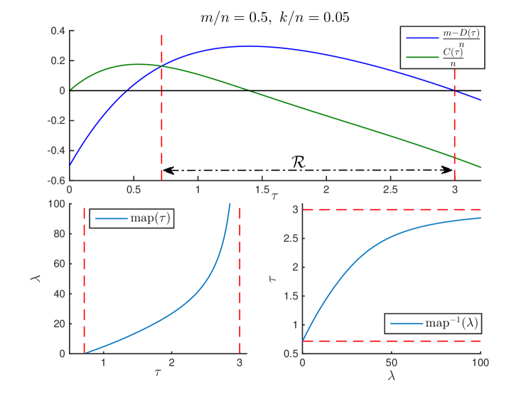
Figure 1: Illustration of the region $\mathcal{R}$ and of the ${\mathrm{map}}$ function (Defn. 2.2) for $f=\|\cdot\|_{1}$ and $\mathbf{x}_{0}\in\mathbb{R}^{n}$ a $k$-sparse vector. ${\mathrm{map}}^{-1}$ maps the value of the regularizer ${\lambda}$ in (1) to a value in $\mathcal{R}$. $D(\tau)$ and $C(\tau)$ are computed as in (10)

.

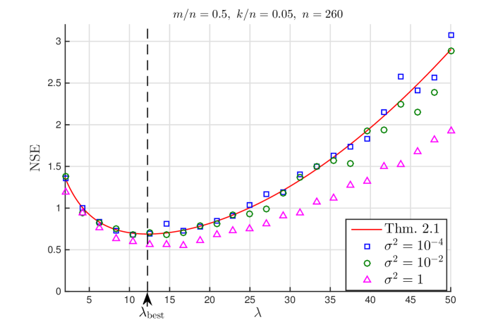
Figure 2: Numerical validation of Theorem II.1 for $f=\|\cdot\|_{1}$ and $\mathbf{x}_{0}\in\mathbb{R}^{n}$ a $k$-sparse vector. Measured values of $\operatorname{NSE}(\sigma)$ are averages over 50 realizations of $\mathbf{A},\mathbf{v}$. The theorem accurately predicts $\operatorname{NSE}(\sigma)$ as $\sigma\rightarrow 0$. Results support our claim that $\operatorname{aNSE}=\operatorname{wNSE}$. ${\lambda}_{best}$ is the value of the optimal regularizer as predicted by Lemma 2.2.

II-C5 On the worst-case NSE

We conjecture that

$$\operatorname{wNSE}:=\sup_{\sigma>0}\operatorname{NSE}(\sigma)=\lim_{\sigma\rightarrow 0}\operatorname{NSE}(\sigma)=:\operatorname{aNSE}.$$ (12)

Theorem II.1 would then imply that for any $\sigma>0$:

$$\lim_{n\rightarrow\infty}\operatorname{NSE}(\sigma)\leq\eta({\lambda}),$$

in probability. There are several reasons that suggest this claim. First, $\operatorname{wNSE}=\operatorname{aNSE}$ has already been shown to hold for algorithms similar to (1) such as: i) the constrained generalized LASSO in (3), [8, 12, 1], ii) the proximal denoiser [18, 19], which is essentially (1) when $m=n$ and $\mathbf{A}=\mathbf{I}_{n}$. Furthermore, our conjecture is supported by computational experiments; see Figure 2 and [1, Sec. 13].

II-C6 Evaluating the bound

Evaluating the bound of Theorem II.1 for particular instances of structures and regularizers requires the ability to compute $D(\tau)$ and $C(\tau)$. It is important to note that this only requires knowledge of the particular structure of the unknown signal $\mathbf{x}_{0}$, and not the explicit unknown signal itself. For example, in sparse recovery, $D({\lambda})$ is the same for all $k$-sparse signals (see (10) and Fig. 1).

II-C7 Optimal tuning

Thm. II.1 suggests a simple recipe for finding the optimal value $\lambda_{\text{best}}$ of the regularizer parameter.

Lemma II.2

Recall $\eta({\lambda})$ as defined in Theorem II.1. Let $\lambda_{\text{best}}:=\arg\min_{{\lambda}\geq 0}\eta({\lambda})$ and $\tau_{\text{best}}:=\arg\min_{\tau\geq 0}D(\tau)$. Then, $\lambda_{\text{best}}=\tau_{\text{best}}\sqrt{m-D(\tau_{\text{best}})}.$

The proof of the lemma is not involved and is omitted for brevity. It is shown in [17, Lem. C.2] that $D(\tau)$ is strictly convex. Thus, $\tau_{\text{best}}$ can be efficiently calculated as the unique solutions to a convex program. This determines $\lambda_{\text{best}}$. Note that even though calculating $\lambda_{\text{best}}$ does not require explicit knowledge of $\mathbf{x}_{0}$ itself, it does assume knowledge of the particular structure. For instance, in sparse recovery we need to know the sparsity level $k$ (see Fig. 2).

II-C8 Phase-transitions

Combining Theorem II.1 with Lemma II.2 it holds with probability one that,

$$\lim_{\sigma\rightarrow 0}\min_{{\lambda}>0}\frac{\|\hat{\mathbf{x}}-\mathbf{x}_{0}\|_{2}^{2}}{\sigma^{2}}=\frac{\min_{\tau}D(\tau)}{m-\min_{\tau}D(\tau)}.$$

In view of the $\operatorname{wNSE}$ conjecture in (21), the quantity in the left hand side can be viewed as the minimax NSE of G-LASSO for a fixed signal $\mathbf{x}_{0}$. While $m>\min_{\tau}D(\tau)$, we can always tune (1) to guarantee robust recovery. However, as the number of measurements $m$ approaches $\min_{\tau}D(\tau)$, then, even after optimal tuning, the NSE grows to $\infty$. This phase-transition characterizing the robustness of (1) is identical to (8), i.e. the phase-transition in noiseless compressed sensing. This observation was first formally predicted in [8], and, later proved in [9] and [12], for $f=\|\cdot\|_{1}$ and $\mathbf{x}_{0}$ k-sparse.

II-C9 Robustness

Theorem II.1 reveals the following interesting feature of (1). Given sufficient number of measurements $m>\min_{\tau}D(\tau)$, the recovery is robust for all choices of the regularizer parameter ${\lambda}>0$. In particular, this is in contrast to the $\ell_{2}$-LASSO in (2). It was shown in [1, 23] that the NSE of the later becomes unbounded if the regularizer parameter is larger than some ${\lambda}_{\max}$.

II-C10 Relevant literature

Most error bounds derived in the literature for (1) are order-wise. The first precise results were derived in the context of sparse recovery via the AMP framework: [8] develops formal expressions for the $\operatorname{wNSE}$ of (1) under optimal tuning of the regularizer parameter ${\lambda}>0$; [9] explicitly characterize $\operatorname{NSE}(\sigma)$ for all values of ${\lambda}>0$ and all $\sigma>0$. The rest of the works that we list here use the GMT framework. [12, 1] precisely characterizes the $\operatorname{wNSE}$ of (3). [1] computes the $\operatorname{aNSE}$ of (2). The $\operatorname{NSE}(\sigma)$ of (2) with $\ell_{1}$-regularization but arbitrary $\sigma>0$ has been characterized by the authors in [24]. Theorem II.1 characterizes the $\operatorname{aNSE}$ of the generalized $\ell_{2}^{2}$-LASSO.

III Proof Outline

We outline the main steps of the proof here. Most of the technical details are deferred to the Appendix. Before everything, we re-write (1) by changing the decision variable to be the error vector ${\mathbf{w}}=\mathbf{x}-\mathbf{x}_{0}$:

$$\hat{\mathbf{w}}:=\min_{{\mathbf{w}}}\frac{1}{2}\|\mathbf{A}{\mathbf{w}}-\sigma\mathbf{v}\|_{2}^{2}+\frac{{\lambda}}{\sigma}f(\mathbf{x}_{0}+{\mathbf{w}}).$$ (13)

Theorem II.1 states a precise expression for the limiting behavior $\lim_{\sigma\rightarrow 0}\|\hat{\mathbf{w}}\|^{2}/\sigma^{2}$. Throughout the analysis, we fix any ${\lambda}>0$. Also, we simply write $\|\cdot\|$ instead of $\|\cdot\|_{2}$.

III-A First-order Approximation

We start with a useful approximation to (13). The idea is that in the regime of interest we expect $\hat{\mathbf{w}}$ to scale linearly with $\sigma$. Thus, in the limit $\sigma\rightarrow 0$, $\|\hat{\mathbf{w}}\|$ is sufficiently small such that $f(\mathbf{x}_{0}+{\mathbf{w}})\approx f(\mathbf{x}_{0})+\sup_{\mathbf{s}\in\partial f(\mathbf{x}_{0})}\mathbf{s}^{T}{\mathbf{w}}$. Note that this always holds with a “$\geq$” sign due to convexity. What we show in the Appendix is essentially that introducing this approximation in (13) does note alter $\|\hat{\mathbf{w}}\|$ in the limit $\sigma\rightarrow 0$.

III-B Gaussian min-max Theorem

We get a handle on (13) and its optimal value via analyzing a different and simpler optimization problem. The machinery that allows this relies on Gordon’s Gaussian min-max theorem (GMT) [13, Lem. 3.1]. In fact, we require a stronger version of the GMT that can be obtained when accompanied with additional convexity assumptions that are not present in its original formulation. The fundamental idea is attributed to Stojnic [12]. [15] builds upon this and derives a concrete and somewhat extended statement of the result in [15, Thm. II.1]. Please refer to the discussion in [15] for further details on the GMT, the role of convexity, and, the differences between [13, Lem. 3.1], [12] and [15, Thm. II.1]. We summarize the result of [15, Thm. II.1] in the next few lines. Let $\mathbf{G}\in\mathbb{R}^{m\times n},\mathbf{g}\in\mathbb{R}^{m},\mathbf{h}\in\mathbb{R}^{n}$ have entries i.i.d. Gaussian; ${\mathcal{S}}_{\mathbf{a}}\subset\mathbb{R}^{n}$,${\mathcal{S}}_{\mathbf{b}}\subset\mathbb{R}^{m}$ be convex compact sets, and $\psi:{\mathcal{S}}_{\mathbf{a}}\times{\mathcal{S}}_{\mathbf{b}}\rightarrow\mathbb{R}$ be convex-concave and continuous. Further consider the following two min-max problems:

$$\Phi(\mathbf{A}):=\min_{\mathbf{a}\in{\mathcal{S}}_{\mathbf{a}}}\max_{\mathbf{b}\in{\mathcal{S}}_{\mathbf{b}}}\mathbf{b}^{T}\mathbf{G}\mathbf{a}+\psi(\mathbf{a},\mathbf{b}),$$ (14)

$${\phi(\mathbf{g},\mathbf{h}):=\min_{\mathbf{a}\in{\mathcal{S}}_{\mathbf{a}}}\max_{\mathbf{b}\in{\mathcal{S}}_{\mathbf{b}}}\|\mathbf{a}\|\mathbf{g}^{T}\mathbf{b}-\|\mathbf{b}\|\mathbf{h}^{T}\mathbf{a}+\psi(\mathbf{a},\mathbf{b}).}$$ (15)

Then, for any $\mu\in\mathbb{R},t>0$:

$${\mathbb{P}}\left(|\Phi(\mathbf{A})-\mu|>t\right)\leq 2{\mathbb{P}}\left(|\phi(\mathbf{g},\mathbf{h})-\mu|>t\right).$$

Thus, if the optimal cost $\phi(\mathbf{g},\mathbf{h})$ of (15) concentrates to some value $\mu$, the same is true for $\Phi(\mathbf{A})$. This suggests analyzing (15) instead of (14), and indirectly yield conclusions for the latter. The premise is that the optimization in (15) is easier to analyze; we often refer to it as “Gordon’s optimization” following [15]. Assuming a setup in which the problem dimensions $m,n$ grow to infinity it is shown in [15] that if $\phi(\mathbf{g},\mathbf{h})$ converges in probability to deterministic value $d_{*}$, then, so is $\Phi(\mathbf{G})$. What is more, if $\|\mathbf{a}_{*}(\mathbf{g},\mathbf{h})\|$ converges to say $\alpha_{*}$, and some appropriate strong convexity assumption on the objective function of (15) is satisfied, then $\|\mathbf{a}_{*}(\mathbf{G})\|$ also converges to $\alpha_{*}$. Here, we have denoted $\mathbf{a}_{*}(\mathbf{g},\mathbf{h})$, $\mathbf{a}_{*}(\mathbf{G})$ for the minimizers in (15) and (14), respectively; refer to [15] and Lemma .2 for the exact statements. As might be already suspected, this latter property is of interest to our problem. In what follows, we bring (1) in the format of (14), derive the corresponding “Gordon’s optimization” problem and analyze the minimizer of that one instead.

III-C Gordon’s Optimization

We use the fact that $(1/2)\|\mathbf{a}\|^{2}=\max_{\mathbf{b}}\mathbf{b}^{T}\mathbf{a}-(1/2)\|\mathbf{b}\|^{2}$ to equivalently express $\hat{\mathbf{w}}$ as the solution to (also, recall the first-order approximation)

$$\min_{{\mathbf{w}}}\max_{\mathbf{b}}\mathbf{b}^{T}\mathbf{A}{\mathbf{w}}-\sigma\mathbf{b}^{T}\mathbf{v}-({1}/{2})\|\mathbf{b}\|^{2}+{\lambda}\max_{\mathbf{s}\in\partial f(\mathbf{x}_{0})}\mathbf{s}^{T}{\mathbf{w}}.$$

Identify $\psi({\mathbf{w}},\mathbf{b})=-\sigma\mathbf{b}^{T}\mathbf{v}-\frac{1}{2}\|\mathbf{b}\|^{2}+{\lambda}\max_{\mathbf{s}}\mathbf{s}^{T}{\mathbf{w}}$, which is convex-concave and continuous, to see that the above is in the desired format (14). The only caveat is that the constraint sets on ${\mathbf{w}}$ and $\mathbf{b}$ appear unbounded. This is appropriately treated in the Appendix and we do not elaborate any further here. The corresponding “Gordon’s optimization” problem writes:

$$\min_{{\mathbf{w}}}\max_{{{\mathbf{s},\mathbf{b}}}}\|{\mathbf{w}}\|\mathbf{g}^{T}\mathbf{b}-\|\mathbf{b}\|\mathbf{h}^{T}{\mathbf{w}}-\sigma\mathbf{b}^{T}\mathbf{v}-\frac{1}{2}\|\mathbf{b}\|^{2}+{\lambda}\mathbf{s}^{T}{\mathbf{w}},$$

where the variable $\mathbf{s}$ is constrained in $\partial f(\mathbf{x}_{0})$, but we omit to shorten notation. In the next lines, we show how to simplify this optimization to a scalar problem. Recall that $\mathbf{g},\mathbf{v}$ both have entries i.i.d. $\mathcal{N}(0,1)$ and are independent of each other; thus $\|{\mathbf{w}}\|\mathbf{g}+\sigma\mathbf{v}$ has entries $\mathcal{N}(0,\sqrt{\|{\mathbf{w}}\|^{2}+\sigma^{2}})$. Also, note that the maximization over the direction of $\mathbf{b}$ is easy to perform, since $\max_{\|\mathbf{b}\|=\beta}\mathbf{g}^{T}\mathbf{b}=\beta\|\mathbf{g}\|$, $\beta\geq 0$. With these, and some abuse of notation so that $\mathbf{g}$ continues being i.i.d standard normal gaussian, we may rewrite the above as:

$$\min_{{\mathbf{w}}}\max_{\mathbf{s},\beta\geq 0}\sqrt{\|{\mathbf{w}}\|^{2}+\sigma^{2}}\|\mathbf{g}\|\beta-(\beta\mathbf{h}-{\lambda}\mathbf{s})^{T}{\mathbf{w}}-{\beta^{2}/2}.$$

Observe that the objective function is now convex in ${\mathbf{w}}$ and concave in $\beta,\mathbf{s}$. Thus, modulo compactness of the constraint sets (see Appendix for details), we can flip the order of minimization and maximization [21, Cor. 37.3.2], and write:

$$\max_{\mathbf{s},\beta\geq 0}\min_{{\mathbf{w}}}\sqrt{\|{\mathbf{w}}\|^{2}+\sigma^{2}}\|\mathbf{g}\|\beta-(\beta\mathbf{h}-{\lambda}\mathbf{s})^{T}{\mathbf{w}}-{\beta^{2}/2}.$$

But, now, it is easy to perform the minimization over the direction of ${\mathbf{w}}$. Doing this, and letting $\alpha$ represent $\|{\mathbf{w}}\|$:

$$\max_{\mathbf{s},\beta\geq 0}\min_{\alpha\geq 0}\sqrt{\alpha^{2}+\sigma^{2}}\|\mathbf{g}\|\beta-\alpha\beta\|\mathbf{h}-\frac{{\lambda}}{\beta}\mathbf{s}\|-{\beta^{2}/2}.$$

We are almost done with the simplifications. One last step amounts to flipping the order of min-max once more (the objective is appropriately concave-convex) and performing the maximization over $\mathbf{s}$, which results in the appearance of the distance term below:

$${\min_{\alpha\geq 0}\max_{\beta\geq 0}\sqrt{\alpha^{2}+\sigma^{2}}\|\mathbf{g}\|\beta-\alpha\text{{dist}}(\mathbf{h},\frac{{\lambda}}{\beta}\partial f(\mathbf{x}_{0}))-{\beta^{2}/2}.}$$ (16)

III-D Analysis of Gordon’s Optimization

In (16), the variable $\alpha$ plays the role of $\|{\mathbf{w}}\|$. Thus, from the discussion in Section III-B, if we find the value to which the optimal $\alpha_{*}(\mathbf{g},\mathbf{h})$ in (16) converges, then, we may conclude that the desired quantity $\|\hat{\mathbf{w}}(\mathbf{A},\mathbf{v})\|$ also converges to the same value. This will establish Theorem II.1. Assume the asymptotic regime that holds for Theorem II.1 We only highlight the main ideas here and defer most of the details to the Appendix.

Both functions $\|\mathbf{g}\|$ and $\text{{dist}}(\mathbf{h},({\lambda}/\beta)\partial f(\mathbf{x}_{0}))$ in (16) are 1-Lipschitz in their arguments. Then, the classical gaussian concentration of Lipschitz functions implies that they concentrate around $\sqrt{m}$ and $\sqrt{D({\lambda}/\beta)}$, respectively (e.g. [1, Lem. B.2]). We use this in the appendix to prove that (16) converges in probability (after proper normalization) to

$$\min_{\alpha\geq 0}\max_{\beta\geq 0}\sqrt{\alpha^{2}+\sigma^{2}}\sqrt{m}\beta-\alpha\beta\sqrt{D({\lambda}/\beta)}-{\beta^{2}/2}.$$ (17)

Moreover, the minimizer of (16) converges to the minimizer $\alpha_{*}$ of the deterministic minimization in (17). To compute $\alpha_{*}$, we use duality (the objective is (strictly) convex in $\alpha$ and concave in $\beta$). First, fix $\beta$, differentiate the objective in (17) w.r.t. $\alpha$ and equate to $0$ to find that is minimized at

$$\alpha_{*}(\beta)=\sqrt{D({\lambda}/\beta)}/\sqrt{m-D({\lambda}/\beta)}.$$

Substituting this value back in (17) and differentiating now with respect to $\beta$, yields the optimal $\beta_{*}={\lambda}/{\mathrm{map}}^{-1}({\lambda})$. Note that $\alpha_{*}(\beta_{*})$ agrees with the expression of the theorem to conclude.

In Section III we outlined the proof of Theorem II.1. Here, we provide a complete proof of the theorem.

-E Preliminaries

We rewrite (1) in a more convenient format for the purposes of the analysis. In particular, (i) substitute $\mathbf{y}=\mathbf{A}\mathbf{x}_{0}+\sigma\mathbf{v}$, (iii) subtract from the objective the constant term ${\lambda}f(\mathbf{x}_{0})$, (ii) change the decision variable to the quantity of interest, i.e. the normalized error vector ${\mathbf{w}_{\sigma}}:=(1/\sigma)({\mathbf{x}-\mathbf{x}_{0}})$, (iv) rescale by a factor of $\sigma^{2}$. Then,

$$\hat{\mathbf{w}}_{\sigma}:=\min_{{\mathbf{w}_{\sigma}}}\frac{1}{2}\|\mathbf{A}{\mathbf{w}_{\sigma}}-\mathbf{v}\|_{2}^{2}+\frac{{\lambda}}{\sigma}(f(\mathbf{x}_{0}+\sigma{\mathbf{w}_{\sigma}})-f(\mathbf{x}_{0})).$$ (18)

We will derive a precise expression for the limiting (as $n\rightarrow\infty$) behavior of $\lim_{\sigma\rightarrow 0}\|\hat{\mathbf{w}}_{\sigma}\|_{2}$. Note that after the normalization of $\mathbf{x}-\mathbf{x}_{0}$ with $\sigma$ , it is not guaranteed that the optimal minimizer in (18) is bounded (think of $\sigma\rightarrow 0$). However, we will prove that in the regime of Theorem II.1 this is indeed the case. Many of the arguments that we use in the analysis require boundedness of the constraint sets. To tackle this, we assume that $\hat{\mathbf{w}}_{\sigma}$ is bounded by some large constant $K>0$ (with probability one over $\mathbf{A},\mathbf{v}$), the value of which to be chosen at the end of the analysis. Recall that at that point we will have a precise characterization of the limiting behavior of $\|\hat{\mathbf{w}}_{\sigma}\|_{2}$, say $\alpha_{*}$. If $\alpha_{*}$ turns out to be independent on the value of $K$ which we started with, then we will assume that this starting value was strictly larger than $\alpha_{*}$. Thus, in what follows, we let $K,\Lambda,M$ denote such (arbitrarily) large, but finite, positive quantities. For $K$, which is reserved as an upper bound on $\|{\mathbf{w}_{\sigma}}\|$ we assume that is constant in the sense that it does not scale with $n$. This will be required when we apply [15, Thm. II.2] in Section -H. On the other hand, $\Lambda,\mathbf{M}$ are in general allowed to depend on $n$. Also, we fix ${\lambda}>0$ and write $\|\cdot\|$ instead of $\|\cdot\|_{2}$.

-F Gordon’s Optimization for arbitrary $\sigma$

We use the fact that

$$(1/2)\|\mathbf{a}\|^{2}=\max_{\mathbf{b}}\mathbf{b}^{T}\mathbf{a}-(1/2)\|\mathbf{b}\|^{2},$$ (19)

to equivalently express $\hat{\mathbf{w}}_{\sigma}$ as the solution to

$$\min_{\|{\mathbf{w}_{\sigma}}\|\leq K}\max_{\|\mathbf{b}\|\leq\Lambda}\mathbf{b}^{T}\mathbf{A}{\mathbf{w}_{\sigma}} -\mathbf{b}^{T}\mathbf{v}-\frac{1}{2}\|\mathbf{b}\|^{2}$$

$$+\frac{{\lambda}}{\sigma}(f(\mathbf{x}_{0}+\sigma{\mathbf{w}_{\sigma}})-f(\mathbf{x}_{0})).$$

In view of (19) and the boundedness of ${\mathbf{w}_{\sigma}}$, the set of optima of $\mathbf{b}$ is also bounded by some $0<\Lambda:=\Lambda(K)<\infty$. This brings (18) in the desired format (14). Then, (15) writes

$$\tilde{\mathbf{w}}_{\sigma}(\mathbf{g},\mathbf{h}) :=\min_{\|{\mathbf{w}_{\sigma}}\|\leq K}\max_{\|\mathbf{b}\|\leq\Lambda}\sqrt{\|{\mathbf{w}_{\sigma}}\|^{2}+1}\mathbf{g}^{T}\mathbf{b}-\|\mathbf{b}\|\mathbf{h}^{T}{\mathbf{w}_{\sigma}}$$

$$\qquad-\|\mathbf{b}\|^{2}/2+({{\lambda}}/{\sigma})(f(\mathbf{x}_{0}+\sigma{\mathbf{w}_{\sigma}})-f(\mathbf{x}_{0})),$$

The maximization over the direction of $\mathbf{b}$ is easy to perform; note that $\max_{\|\mathbf{b}\|=\beta}\mathbf{g}^{T}\mathbf{b}=\beta\|\mathbf{g}\|_{2},\beta\geq 0$. Also, $f$ is continuous and convex, thus, we can express it in terms of its convex conjugate $f^{*}(\mathbf{u})=\sup_{\mathbf{x}}\mathbf{u}^{T}\mathbf{x}-f(\mathbf{x})$. In particular, applying [21, Thm.12.2] we have $f(\mathbf{x}_{0}+\sigma{\mathbf{w}_{\sigma}})=\sup_{\mathbf{u}}\mathbf{x}_{0}^{T}\mathbf{u}+\sigma\mathbf{u}^{T}{\mathbf{w}_{\sigma}}-f^{*}(\mathbf{u})$. The supremum here is achieved at $\mathbf{u}_{*}\in\partial f(\mathbf{x}_{0}+\sigma{\mathbf{w}_{\sigma}})$ [21, Thm. 23.5]. Also, from [25, Prop. 4.2.3], $\cup_{\|{\mathbf{w}_{\sigma}}\|\leq K}\partial f(\mathbf{x}_{0}+\sigma{\mathbf{w}_{\sigma}})$ is bounded. Thus, the set of maximizers $\mathbf{u}_{*}$ is bounded and for some $0<M:=M(K)<\infty$, $\tilde{\mathbf{w}}_{\sigma}$ is given as the solution to

$$\phi(\sigma;\mathbf{g},\mathbf{h}):=\min_{\|{\mathbf{w}_{\sigma}}\|\leq K}\max_{\begin{subarray}{c}0\leq\beta\leq\Lambda\\ 0\leq\|\mathbf{u}\|\leq M\end{subarray}}\sqrt{\|{\mathbf{w}_{\sigma}}\|^{2}+1}\|\mathbf{g}\|\beta-{\beta^{2}}/{2}$$

$$~{}~{}~{}-(\beta\mathbf{h}-{\lambda}\mathbf{u})^{T}{\mathbf{w}_{\sigma}}+\frac{{\lambda}}{\sigma}(\mathbf{u}^{T}\mathbf{x}_{0}-f^{*}(\mathbf{u})-f(\mathbf{x}_{0})).$$ (20)

-G Gordon’s Optimization in the limit $\sigma\rightarrow 0$

[15, Thm. II.2] relates $\|\tilde{\mathbf{w}}_{\sigma}\|$ to $\|\hat{\mathbf{w}}_{\sigma}\|$, under appropriate assumptions. Also, recall that we wish to characterize $\lim_{\sigma\rightarrow 0}\|\hat{\mathbf{w}}_{\sigma}\|$. Thus, in view of (-F) we wish to analyze the problem

$$\phi_{0}:=\phi_{0}(\mathbf{g},\mathbf{h}):=\lim_{\sigma\rightarrow 0}\phi(\sigma;\mathbf{g},\mathbf{h}).$$

In (-F), from Fenchel’s inequality:

$$\mathbf{u}^{T}\mathbf{x}_{0}-f^{*}(\mathbf{u})-f(\mathbf{x}_{0})\leq 0.$$ (21)

With this observation, we prove in the next lemma that $\phi(\sigma;\mathbf{g},\mathbf{h})$ is non-decreasing in $\sigma$; see Section -I for the proof.

Lemma .1

Fix $\mathbf{g},\mathbf{h}$ and consider $\phi(\cdot;\mathbf{g},\mathbf{h}):(0,\infty)\rightarrow\mathbb{R}$ as defined in (-F). $\phi(\sigma;\mathbf{g},\mathbf{h})$ is non-decreasing in $\sigma$.

In particular, when viewed as a function of $\kappa:={\lambda}/\sigma$, $\phi(\cdot;\mathbf{g},\mathbf{h})$ is non-increasing. Thus,

$$\phi_{0}=\lim_{\sigma\rightarrow 0}\phi(\sigma)=\lim_{\kappa\rightarrow\infty}\phi(\kappa)=\inf_{\kappa\geq 0}\phi(\kappa),$$ (22)

Next, we argue that we can flip the order of min-max; we will apply [21, Cor. 37.3.2]. The objective function in (-F) is continuous, convex in both ${\mathbf{w}_{\sigma}},\kappa$, and, concave both in $\mathbf{b},\mathbf{u}$. The constraint sets are all convex and one of them is bounded. With this and (22), we get

$$\phi_{0}(\mathbf{g},\mathbf{h})=\max_{\begin{subarray}{c}0\leq\beta\leq\Lambda\\ 0\leq\|\mathbf{u}\|\leq M\end{subarray}}\min_{\|{\mathbf{w}_{\sigma}}\|\leq K}\inf_{\kappa\geq 0}\sqrt{\|{\mathbf{w}_{\sigma}}\|^{2}+1}\|\mathbf{g}\|\beta-\frac{\beta^{2}}{2}$$

$$~{}~{}~{}~{}-(\beta\mathbf{h}-{\lambda}\mathbf{u})^{T}{\mathbf{w}_{\sigma}}+\kappa(\mathbf{u}^{T}\mathbf{x}_{0}-f^{*}(\mathbf{u})-f(\mathbf{x}_{0})).$$ (23)

Recall (21) and the fact that equality is achieved iff $\mathbf{u}\in\partial f(\mathbf{x}_{0})$ (e.g. [21, Thm. 23.5]). Then, $\phi_{0}(\mathbf{g},\mathbf{h})$ is given by

$$\max_{\begin{subarray}{c}0\leq\beta\leq\Lambda\\ \mathbf{u}\in\partial f(\mathbf{x}_{0})\end{subarray}}\min_{\|{\mathbf{w}_{\sigma}}\|\leq K}\sqrt{\|{\mathbf{w}_{\sigma}}\|^{2}+1}\|\mathbf{g}\|\beta-(\beta\mathbf{h}-{\lambda}\mathbf{u})^{T}{\mathbf{w}_{\sigma}}-\frac{\beta^{2}}{2},$$

where we have assumed $\infty>M>\max_{\mathbf{s}\in\partial f(\mathbf{x}_{0})}\|\mathbf{s}\|$. We can simplify this one step further by performing the minimization over the direction of ${\mathbf{w}_{\sigma}}$. In the problem below note that $\alpha$ plays the role of $\|{\mathbf{w}_{\sigma}}\|$. Thus, $\phi_{0}(\mathbf{g},\mathbf{h})=\max_{\begin{subarray}{c}0\leq\beta\leq\Lambda\\ \mathbf{u}\in\partial f(\mathbf{x}_{0})\end{subarray}}\min_{0\leq\alpha\leq K}\sqrt{\alpha^{2}+1}\|\mathbf{g}\|\beta-\alpha\|\beta\mathbf{h}-{\lambda}\mathbf{u}\|-\frac{\beta^{2}}{2}.$ The objective function above is continuous, convex in $\alpha$ and concave in $\beta,\mathbf{u}$. Also the constraint sets are convex and bounded. Thus, [21, Cor. 37.3.2], we can flip the order of max-min. Also, for $\beta>0$, $\min_{\mathbf{u}\in\partial f(\mathbf{x}_{0})}\|\beta\mathbf{h}-{\lambda}\mathbf{u}\|=\beta\text{{dist}}(\mathbf{h},({\lambda}/\beta)\partial f(\mathbf{x}_{0}))$. With these, normalizing with $1/m$ and appropriately rescaling $\beta$:

$$\tilde{\phi}_{0}(\mathbf{g},\mathbf{h})=\min_{0\leq\alpha\leq K}\max_{0\leq\beta\leq\Lambda}{\mathcal{L}}(\alpha,\beta;\mathbf{g},\mathbf{h}):=$$

$$\quad\sqrt{\alpha^{2}+1}\frac{\|\mathbf{g}\|}{\sqrt{m}}\beta-\alpha\beta\frac{1}{\sqrt{m}}\text{{dist}}(\mathbf{h},\frac{{\lambda}}{\beta\sqrt{m}}\partial f(\mathbf{x}_{0}))-\frac{\beta^{2}}{2}.$$ (24)

Normalization here is convenient for the purposes of applying statement (iii) of [15, Thm. II.2], which follows.

-H Applying [15, Thm. II.2]

(-G) describes “Gordon’s optimization” (modulo normalization with $m$) corresponding to (18) in the limit of $\sigma\rightarrow 0$. Also, the variable $\alpha$ in (-G) plays the role of $\|{\mathbf{w}_{\sigma}}\|$. The idea is that problem (-G) behaves in the large system limit just like (18). This is formalized in the lemma below, which is a direct corollary of [15, Thm. II.2] applied to our setup and combined with our analysis thus far. For the statement of the lemma recall that we are operating in the large-system limit in which problem dimensions $n,m,\min_{\tau\geq 0}D(\tau)$ grow linearly to infinity (cf. Section II-B1). Also, we use standard notation $X_{n}\xrightarrow{P}c$, to denote convergence in probability of $\{X_{n}\}_{n=1}^{\infty}$ to $c\in\mathbb{R}$ as $n\rightarrow\infty$.

Lemma .2

Let $\hat{\mathbf{w}}_{\sigma}$ and $\mathrm{Cost}_{\sigma}$ be a minimizer and the optimal cost of (18), respectively. Also, recall (-G). Suppose $d:[0,\infty)\rightarrow\mathbb{R}$ is such that $\max_{0\leq\beta\leq\Lambda}{\mathcal{L}}(\alpha,\beta;\mathbf{g},\mathbf{h})\xrightarrow{P}d(\alpha)$ for all $\alpha\in[0,K]$, and $d(\alpha)\geq d(\alpha_{*})+\zeta(\alpha-\alpha_{*})^{2},\forall\alpha\in[0,K]$, for some $\alpha_{*}\in[0,K]$ and $\zeta>0$. Then,

$$\lim_{\sigma\rightarrow 0}\|\hat{\mathbf{w}}_{\sigma}\|_{2}\xrightarrow{P}\alpha_{*}\quad\text{ and }\quad\lim_{\sigma\rightarrow 0}\frac{\mathrm{Cost}_{\sigma}}{\sigma^{2}m}\xrightarrow{P}d(\alpha_{*}).$$ (25)

Recall $\hat{\mathbf{w}}_{\sigma}=(\hat{\mathbf{x}}-\mathbf{x}_{0})/\sigma$, thus, $\|\hat{\mathbf{w}}_{\sigma}\|^{2}=\operatorname{NSE}(\sigma)$. In what follows, we construct deterministic function $d$ that satisfies the requirements of Lemma .2 and prove that $\alpha_{*}$ satisfies the formula of Theorem II.1. This will complete the proof. To suppress notation, define $({\lambda}_{\beta}):={\lambda}/(\beta\sqrt{m})$.

Both functions $\|\mathbf{g}\|$ and $\text{{dist}}(\mathbf{h},({\lambda}_{\beta})\partial f(\mathbf{x}_{0}))$ are 1-Lipschitz in their arguments. Then, the classical gaussian concentration of Lipschitz functions implies that they concentrate around $\sqrt{m}$ and $\sqrt{D({\lambda}_{\beta})}$, respectively

From standard concentration results on Lipschitz functions of gaussian r.v.s. (e.g. [1, Lem. B.2]), we have for all $\alpha,\beta$:

$${\mathcal{L}}(\alpha,\beta;\mathbf{g},\mathbf{h})\xrightarrow{P}\tilde{d}(\alpha,\beta):=\sqrt{\alpha^{2}+1}\beta-\alpha\beta\sqrt{\frac{D({\lambda}_{\beta})}{m}}-\frac{\beta^{2}}{2}.$$ (26)

As we have seen ${\mathcal{L}}(\alpha,\beta;\mathbf{g},\mathbf{h})$ is convex in $\alpha$ and concave in $\beta$. Since taking limits preserves convexity, the same is true for $\tilde{d}(\alpha,\beta)$. Next, define

$$d(\alpha):=\max_{0\leq\beta\leq\Lambda}\tilde{d}(\alpha,\beta).$$

We claim that this satisfies the prerequisites of Lemma .2.

First, we show the convergence part. It suffices to prove that for each $\alpha$ the convergence in (26) holds uniformly over all $\beta\in[0,\Lambda]$. Concavity of ${\mathcal{L}}(\alpha,\beta)$ in its second argument is critical. In particular, the claim follows from [26, Cor. II.1]: “point-wise convergence in probability of concave functions implies uniform convergence in compact spaces”.

Next, we compute appropriate $\alpha_{*}$. Consider

$$(\alpha_{*},\beta_{*}):=\arg\min_{0\leq\alpha\leq K}\max_{0\leq\beta\leq\Lambda}\tilde{d}(\alpha,\beta)$$ (27)

We compute those in the next lemma; see Section -I for a proof.

Lemma .3

Consider the optimization in (27). Let

$$\alpha_{*}=\sqrt{\frac{D({\mathrm{map}}^{-1}({\lambda}))}{m-D({\mathrm{map}}^{-1}({\lambda}))}}\text{ and }\beta_{*}=\frac{{\lambda}}{{\mathrm{map}}^{-1}({\lambda})\sqrt{m}}.$$

Then, there exist $K,\Lambda$ satisfying $0<\alpha_{*}<K<\infty$ and $0<\beta_{*}<\Lambda<\infty$, such that $(\alpha_{*},\beta_{*})$ are optimal in (27).

Let $K,\Lambda$ in (27) be as in Lemma .3. It remains to prove $d(\alpha)>d(\alpha_{*})+\zeta(\alpha-\alpha_{*})^{2}$ for some $\zeta>0$. Fix $\alpha\in[0,K]$. Clearly,

$$d(\alpha)=\max_{\beta}\tilde{d}(\alpha,\beta)\geq\tilde{d}(\alpha,\beta_{*}).$$

We will now use the fact that for fixed $\beta\in(0,\Lambda]$, the function $\tilde{d}(\alpha,\beta)$ is strongly convex in $0\leq\alpha\leq K$. Indeed,

$${\partial^{2}{\tilde{d}}}/{\partial\alpha^{2}}=\beta/{(\alpha^{2}+1)^{3/2}}\geq\beta/{(K^{2}+1)^{3/2}}.$$

Recall $\beta_{*}>0$ and let $\zeta=\beta_{*}/{(K^{2}+1)^{3/2}}>0$. Then,

$$d(\alpha)\geq\tilde{d}(\alpha,\beta_{*})\geq\tilde{d}(\alpha_{*},\beta_{*})+\zeta(\alpha-\alpha_{*})^{2}.$$

-I Proofs of Auxiliary Results

-I1 Lemma .1

Denote ${\mathcal{L}}(\sigma,{\mathbf{w}_{\sigma}},\beta,\mathbf{u})$ the objective function in (-F) and consider $0<\sigma_{1}<\sigma_{2}<\infty$. Let ${\mathbf{w}_{\sigma}}^{(2)}$ be an optimal solution to the min-max problem in (-F) for $\sigma_{2}$. Then, let $(\beta^{(1)},\mathbf{u}^{(1)})=\arg\max_{\beta,\mathbf{u}}{\mathcal{L}}(\sigma_{1},{\mathbf{w}_{\sigma}}^{(2)},\beta,\mathbf{u})$. Clearly,

$$\phi(\sigma_{1})\leq{\mathcal{L}}(\sigma_{1},{\mathbf{w}_{\sigma}}^{(2)},\beta^{(1)},\mathbf{u}^{(1)}).$$

Using ${\lambda}/\sigma_{1}>{\lambda}/\sigma_{2}$ and (21),

$${\mathcal{L}}(\sigma_{1},{\mathbf{w}_{\sigma}}^{(2)},\beta^{(1)},\mathbf{u}^{(1)})\leq{\mathcal{L}}(\sigma_{2},{\mathbf{w}_{\sigma}}^{(2)},\beta^{(1)},\mathbf{u}^{(1)})$$

But,

$${\mathcal{L}}(\sigma_{2},{\mathbf{w}_{\sigma}}^{(2)},\beta^{(1)},\mathbf{u}^{(1)})\leq\phi(\sigma_{2}).$$

Combine the above chain of inequalities to conclude.

-I2 Lemma .3

Let $\beta_{*},\alpha_{*}$ be as in the statement of the lemma. Also $\tau_{*}:={\mathrm{map}}^{-1}({\lambda})>0$ (cf. Definition II.2). Notice that $\alpha_{*},\beta_{*}>0$ and set

$$0<K=2\alpha_{*}<\infty\quad\text{ and }\quad 0<\Lambda=2\beta_{*}<\infty.$$

As we have seen $\tilde{d}(\alpha,\beta)$ is convex-concave. Also, the constraint sets are convex and compact, hence,

$$(\alpha_{*},\beta_{*})=\max_{0\leq\beta\leq\Lambda}\min_{0\leq\alpha\leq K}\tilde{d}(\alpha,\beta).$$

We have $0<\beta_{*}<\Lambda$ and $D({\lambda}_{\beta_{*}})<m$ and $D({\lambda}_{\beta})$ continuous in $\beta$ (cf. [1, Lem. 8.1]). Thus, there exists open neighborhood $\mathcal{N}_{1}\subset[0,\Lambda]$ such that $D({\lambda}_{\beta})<m,\forall\beta\in\mathcal{N}_{1}$. Fix any such $\beta\in\mathcal{N}_{1}$ and let

$$d_{*}(\beta):=\min_{0\leq\alpha\leq K}\tilde{d}(\alpha,\beta).$$ (28)

Differentiating with respect to $\alpha$, we find

$$\frac{\partial{\tilde{d}}}{{\partial\alpha}}=\beta\frac{\alpha}{\sqrt{\alpha^{2}+1}}-\beta\sqrt{\frac{{D({\lambda}_{\beta})}}{{m}}}.$$

It can be checked that $\alpha_{*}(\beta)=\sqrt{\frac{D({\lambda}_{\beta})}{m-D({\lambda}_{\beta})}}$ is the unique solution to the equation ${\partial{\tilde{d}}}/{{\partial\alpha}}=0$. In particular, $\alpha_{*}=\alpha_{*}(\beta_{*})$ and is feasible, i.e. $\alpha_{*}(\beta_{*})\in(0,K)$. From continuity of $D(\cdot)$ (cf. [1, Lem. 8.1]), we have $\alpha_{*}(\beta)$ be a continuous function of $\beta$. Hence, there exists open neighborhood of $\beta_{*}$, say $\mathcal{N}_{2}\subset\mathcal{N}_{1}$, such that $\alpha_{*}(\beta)\in(0,K)$ for all $\beta\in\mathcal{N}_{2}$. For any such $\beta\in\mathcal{N}_{2}$, $\alpha_{*}(\beta)$ satisfies first-order optimality conditions of the convex minimization in (28), thus, is optimal:

$$d_{*}(\beta)=-{\beta^{2}}/{2}+\frac{\beta}{\sqrt{m}}\sqrt{m-D({\lambda}_{\beta})},~{}~{}\forall\beta\in\mathcal{N}_{2}.$$

Differentiating this with respect to $\beta$ finds:

$$\frac{\partial{d_{*}}}{\partial\beta}=-\beta+\frac{1}{\sqrt{m}}\frac{m-D({\lambda}_{\beta})-C({\lambda}_{\beta})}{\sqrt{m-D({\lambda}_{\beta})}},$$

where we have used $\partial D(\tau)/\partial\tau=-(2/\tau){C(\tau)},\tau>0$ (cf.[17, Lem. C.2]). Note that the second summand above is equal to $\frac{\beta}{{\lambda}}{\mathrm{map}}({\lambda}/(\beta\sqrt{m}))$. With this, it is easy to verify that $\beta_{*}$ is such that $\partial{d_{*}}/\partial\beta=0$. From (28), $d_{*}(\beta)$ is concave as the point-wise minimum of concave functions. Thus, first-order optimality conditions satisfied by $\beta_{*}$ are sufficient, which completes the proof.

References

- [1] S. Oymak, C. Thrampoulidis, and B. Hassibi, “The squared-error of generalized lasso: A precise analysis,” arXiv preprint arXiv:1311.0830, 2013.
- [2] R. Tibshirani, “Regression shrinkage and selection via the lasso,” Journal of the Royal Statistical Society. Series B (Methodological), pp. 267–288, 1996.
- [3] A. Belloni, V. Chernozhukov, and L. Wang, “Square-root lasso: pivotal recovery of sparse signals via conic programming,” Biometrika, vol. 98, no. 4, pp. 791–806, 2011.
- [4] E. J. Candes, J. K. Romberg, and T. Tao, “Stable signal recovery from incomplete and inaccurate measurements,” Communications on pure and applied mathematics, vol. 59, no. 8, pp. 1207–1223, 2006.
- [5] E. Candes and T. Tao, “The dantzig selector: Statistical estimation when p is much larger than n,” The Annals of Statistics, pp. 2313–2351, 2007.
- [6] P. J. Bickel, Y. Ritov, and A. B. Tsybakov, “Simultaneous analysis of lasso and dantzig selector,” The Annals of Statistics, vol. 37, no. 4, pp. 1705–1732, 2009.
- [7] S. N. Negahban, P. Ravikumar, M. J. Wainwright, and B. Yu, “A unified framework for high-dimensional analysis of -estimators with decomposable regularizers,” Statistical Science, vol. 27, no. 4, pp. 538–557, 2012.
- [8] D. L. Donoho, A. Maleki, and A. Montanari, “The noise-sensitivity phase transition in compressed sensing,” Information Theory, IEEE Transactions on, vol. 57, no. 10, pp. 6920–6941, 2011.
- [9] M. Bayati and A. Montanari, “The lasso risk for gaussian matrices,” Information Theory, IEEE Transactions on, vol. 58, no. 4, pp. 1997–2017, 2012.
- [10] A. Maleki, L. Anitori, Z. Yang, and R. G. Baraniuk, “Asymptotic analysis of complex lasso via complex approximate message passing (camp),” Information Theory, IEEE Transactions on, vol. 59, no. 7, pp. 4290–4308, 2013.
- [11] C. A. Metzler, A. Maleki, and R. G. Baraniuk, “From denoising to compressed sensing,” arXiv preprint arXiv:1406.4175, 2014.
- [12] M. Stojnic, “A framework to characterize performance of lasso algorithms,” arXiv preprint arXiv:1303.7291, 2013.
- [13] Y. Gordon, On Milman’s inequality and random subspaces which escape through a mesh in . Springer, 1988.
- [14] R. Vershynin, “Introduction to the non-asymptotic analysis of random matrices,” arXiv preprint arXiv:1011.3027, 2010.
- [15] C. Thrampoulidis, S. Oymak, and B. Hassibi, “The Gaussian min-max theorem in the presence of convexity,” arXiv preprint arXiv:1408.4837, 2014.
- [16] V. Chandrasekaran, B. Recht, P. A. Parrilo, and A. S. Willsky, “The convex geometry of linear inverse problems,” Foundations of Computational Mathematics, vol. 12, no. 6, pp. 805–849, 2012.
- [17] D. Amelunxen, M. Lotz, M. B. McCoy, and J. A. Tropp, “Living on the edge: A geometric theory of phase transitions in convex optimization,” arXiv preprint arXiv:1303.6672, 2013.
- [18] D. L. Donoho and I. M. Johnstone, “Minimax risk overl p-balls forl p-error,” Probability Theory and Related Fields, vol. 99, no. 2, pp. 277–303, 1994.
- [19] S. Oymak and B. Hassibi, “Sharp mse bounds for proximal denoising,” arXiv preprint arXiv:1305.2714, 2013.
- [20] Y. Wu and S. Verdú, “Optimal phase transitions in compressed sensing,” Information Theory, IEEE Transactions on, vol. 58, no. 10, pp. 6241–6263, 2012.
- [21] R. T. Rockafellar, Convex analysis. Princeton university press, 1997, vol. 28.
- [22] M. Stojnic, “Various thresholds for -optimization in compressed sensing,” arXiv preprint arXiv:0907.3666, 2009.
- [23] C. Thrampoulidis, S. Oymak, and B. Hassibi, “Simple error bounds for regularized noisy linear inverse problems,” Information Theory, 2014. f 2014. Proceedings. International Symposium on, pp. 3007–3011, 2014.
- [24] C. Thrampoulidis, A. Panahi, D. Guo, and B. Hassibi, “Precise error analysis of the -lasso,” in 40th IEEE International Conference on Acoustics, Speech and Signal Processing (ICASSP) 2015, available on arXiv:1502.04977, 2015.
- [25] D. P. Bertsekas, A. Nedić, and A. E. Ozdaglar, Convex analysis and optimization. Athena Scientific Belmont, 2003.
- [26] P. K. Andersen and R. D. Gill, “Cox’s regression model for counting processes: a large sample study,” The annals of statistics, pp. 1100–1120, 1982.