Low-temperature spin-glass behavior in a diluted dipolar Ising system

Abstract

Using Monte Carlo simulations, we study the character of the spin-glass (SG) state of a site-diluted dipolar Ising model. We consider systems of dipoles randomly placed on a fraction $x$ of all $L^{3}$ sites of a simple cubic lattice that point up or down along a given crystalline axis. For $x\lesssim 0.65$ these systems are known to exhibit an equilibrium spin-glass phase below a temperature $T_{sg}\propto x$. At high dilution and very low temperatures, well deep in the SG phase, we find spiky distributions of the overlap parameter $q$ that are strongly sample-dependent. We focus on spikes associated with large excitations. From cumulative distributions of $q$ and a pair correlation function averaged over several thousands of samples we find that, for the system sizes studied, the average width of spikes, and the fraction of samples with spikes higher than a certain threshold does not vary appreciably with $L$. This is compared with the behavior found for the Sherrington-Kirkpatrick model.

I Introduction

Complex systems are present in life and social sciences, information systems, and economics. page In these systems, different random distributions of their microscopic constituent parts give rise to diverse values of some macroscopic properties.complexity A paradigmatic model in statistical physics that exhibits complexity is the Sherrington-Kirkpatrick (SK) model, sk where the couplings between any pair of spins is randomly fixed to be ferromagnetic (FM) or antiferromagnetic (AF) regardless of the spin-spin distance. This model has both quenched spatial-disorder and frustration,frustration the two essential ingredients of spin glasses (SG).bookstein ; bookmezard Its exact solution solutionSK shows the existence of replica symmetry breaking (RSB):rsb different identical replicas of a sample ${\cal J}$ with the same couplings may, in the thermodynamic limit, stay trapped in different states within the set of infinitely many pure states. These pure states are diverse, in the sense that they are sample-dependent. The distribution of the overlap $q$ between states of a given sample, $p_{\cal J}(q)$, is found to be a comb-like superposition of infinitely many $\delta$-like spikes. In the macroscopic limit, after averaging over spatial disorder, the overlap distribution is given by $p(q)=\delta(q-q_{m})+f(q)$ where $f(q)$ is a non-zero smooth function for $q<q_{m}$ and zero otherwise.

Whether the RSB picture describes correctly the behavior of realistic spin glasses, such as dilute metallic alloys or concentrated insulators binderREV is still a matter of debate. The 3D Edwards-Anderson model (EA),ea in which only nearest-neighbor spins interact, is the simplest one with the essential ingredients of short-ranged SGs. No exact solution exists for the EA model, but there is consensus on the existence of a SG phase based on numerical simulations.oldEA The applicability of a RSB scenario to the SG phase of the EA model is still controversial.newman-stein In the so-called droplet picture, the SG phase is described in terms of a unique state (paired with the one obtained by a global spin inversion) with excitations that are compact droplets of the inverted state. droplet According to this scenario, $p_{\cal J}(q)$ distributions do not exhibit diversity —in the sense that $p_{\cal J}(q)$ is independent of $\cal J$— and the averaged $p(q)$ becomes a single delta function $\delta(q-q_{m})$: $p(q)$ is said to be trivial. Some trivial-non-trivial scenarios, between the droplet and RSB pictures, have also been proposed. kp Early MC simulations point to a non-trivial scenario, kpy but it has been found that the asymptotic behavior for $p(q\simeq 0)$ is only reached at very large sizes even for toy droplet models. toydroplet

There is growing interest in the study of sample-to-sample fluctuations of $p_{\cal J}(q)$ from their average $p(q)$.tutti Some recently proposed quantities give information on the height yucesoy and average widthpcf of spikes found in $p_{\cal J}(q)$. By MC simulations, these quantities have been found to be nearly size-independent for the EA model, in contradiction with RSB predictions. However, these results have been criticized to be far away from the asymptotic regime.critico ; billoire Some have found more useful to study the statistics of the area under $p_{\cal J}(q)$ for $q<q_{m}$.tutti ; billoire The numerical study of SG models distinct from the SK and EA models has shed some light on the virtues and weaknesses of these new probes for measuring diversity. middleton13 ; wittmann

Frustration in the SK and EA models comes from the competition between randomly distributed FM and AF couplings. However, frustration may also appear in fully occupied systems with no quenched disorder, such as the Ising model with pure AF interactions on a FCC lattice.henley Dipoles packed in crystalline arrangements have frustration, exhibiting magnetic order that is strongly dependent on the lattice structure. tisza ; tisza2 Some ferroelectrics luo and magnetic insulators such as LiHoF₄ are known to be well described by arrays of parallel Ising dipoles that behave as uniaxial ferromagnets. holmio In dipolar Ising systems (DIS), dilution put together with the built in geometric frustration results in SG behavior. vil LiHo_xY_1-xF₄ is one example that has been extensively studied. ExperimentsexperimentsHO have found a SG phase for concentration $x=0.16$, and a FM phase for $x>x_{c}$ where $x_{c}\simeq 0.25$. Recent MC simulations of systems of classical Ising dipoles placed on a fraction $x$ of the sites of the LiHoF₄ tetragonal lattice have found a SG phase for all $0<x\lesssim 0.25$ for temperatures below a SG transition temperature $T_{sg}\propto x$. tam ; andresen

Here we study a site-diluted system of $L^{3}$ dipoles, which are placed at random on a fraction $x$ of the sites of a simple cubic (SC) lattice and point up or down along one of the principal axis. In the limit of low concentrations details of the lattice are expected to become irrelevant. Therefore, our model at low concentrations has direct connection with the experimental and numerical work mentioned above. In previous MC work ourPAD we have calculated the entire diagram of the system and found a SG phase for $0<x<x_{c}$ where $x_{c}\simeq 0.65$ with the SG transition temperature given by $T_{sg}(x)\simeq x$. We found from the following evidence that the SG phase behaves marginally: (i) the mean values $q_{1}=<|q|>$ decrease algebraically with $L$ , (ii) averaged overlap distributions of $q/q_{1}$ appear wide and independent of $L$, (iii) $\xi_{L}/L$, where $\xi_{L}$ is a correlation length,cara rises with $L$ at constant $T$, but extrapolates to finite values as $1/L\to 0$. All of this is consistent with quasi-long-range order in the SG phase, Neither the droplet model nor a RSB scenario fit with this marginal behavior.

The main aim of this paper is to study whether diversity may emerge in this geometrically frustrated model at low temperatures and high dilution, rather deep in its marginal SG phase by using the probes for measuring diversity, in the sense that was specified above. The paper is organized as follows. In Sec. II we define the model, give details on the parallel tempered Monte Carlo (TMC) algorithm, tempered and define the quantities we compute. We present results in Sec. III, followed by concluding remarks in Sec. IV.

II model, method, and measured quantities

II.1 Models

We consider site-diluted systems of classical Ising spins on a SC lattice. All spins are parallel and point along the $z$ axis of the lattice. At each lattice site a spin is placed with probability $x$. These spins are coupled solely by dipolar interactions. The Hamiltonian is given by

$${\cal H}=\sum_{<i,j>}T_{ij}\sigma_{i}\sigma_{j},$$ (1)

where the summation runs over all pairs of occupied sites $i$ and $j$ except $i=j$, $\sigma_{i}=\pm 1$ on any occupied site $i$,

$$T_{ij}=\varepsilon_{a}(a/r_{ij})^{3}(1-3z_{ij}^{2}/r_{ij}^{2}),$$ (2)

where $r_{ij}$ is the distance between $i$ and $j$ sites, $z_{ij}$ is the $z$ component of $r_{ij}$, $\varepsilon_{a}$ is an energy, and $a$ is the SC lattice constant. In the following, temperatures shall be given in terms of $\varepsilon_{a}/k_{B}$.

Note that $T_{ij}$ values are not distributed at random, but depend only on the orientation of vectors ${\bf r}_{ij}$ on a SC lattice. This is why DIS exhibit AF order at concentrations $x>x_{c}$. tisza2 ; ourPAD . This is to be contrasted with random-axes dipolar models,rads in which Ising spins point along directions that are chosen at random, introducing randomness on bond strengths.

In this paper we study DIS with $x<<x_{c}$ for which the details of the lattice structure are not important. Not surprisingly, in the limit of high dilution the behavior of DIS and the $LiHo_{x}Y_{4-x}F_{4}$ system (a well known dipolar ferromagnet for $x=1$) have been found to be closely related. ourPAD ; andresen

For comparison, we study also the SK model: a set of $N=L^{3}$ Ising spins $\sigma_{i}=\pm 1$ with interaction energies between any pair of spins at sites $i$ and $j$ given by $J_{ij}\sigma_{i}\sigma_{j}$ with $J_{ij}=\pm 1/\sqrt{N}$ chosen randomly, without bias, for all $ij$ site pairs.

II.2 Method

For the models described in Sec. II.1 we have simulated a large number $N_{s}$ of independent samples. By a sample, $\cal J$, we mean a system with a given quenched distribution of empty sites for DIS (a quenched distribution of random couplings $J_{ij}$ for the SK model). The number of samples we average over is given in Tables I and II. We have tried not to make $N_{s}$ smaller with increasing $L$. This is because statistical errors are independent of $L$, because of non-self-averaging. (However, for DIS with $L=10$, we could only do $1.2\times 10^{4}$ samples. That took an Intel 8-core Xeon processor E5-2670 some $60$ years worth of CPU time).

Thermal averages come from averaging over the time range $[t_{0},2t_{0}]$, where $t_{0}$ is the equilibration time. We further average over the $N_{s}$ samples with different realizations of quenched disorder.

In order to accelerate equilibration at low temperatures in the glassy phase we use a parallel tempered Monte Carlo (TMC) algorithm.tempered We apply the TMC algorithm as follows. We run in parallel a set of $n$ identical replicas of each sample at different temperatures in the interval $[T_{min},T_{max}]$ with a separation $\Delta$ between neighboring temperatures. Each replica starts from a completely disordered spin configuration $\{\sigma_{i}\}$. We apply the TMC algorithm to any given sample in two stages. In the first stage, the $n$ replicas of the sample $\cal J$ evolve independently for $10$ MC Metropolis sweeps.mc All dipolar fields throughout the system are ufated every time a spin flip is accepted. In the second stage, we give any pair of replicas evolving at temperatures $T$ and $T-\Delta$ a chance to exchange states between them following standard tempering rules which satisfy detailed balance. tempered These exchanges allow all replicas to diffuse back and forth from low to high temperatures and reduce equilibration times for the rough energy landscapes of SGs. We find it helpful to have the highest temperature $T_{max}$ larger than $1.6\times T_{sg}$. We choose $\Delta$ such that at least $30\%$ of all attempted exchanges are accepted for all $T$.

For DIS we use periodic boundary conditions (PBC). Details of the PBC scheme we use can be found in Ref. ourPAD . We let a spin on an occupied site $i$ interact only with spins within an $L\times L\times L$ cube centered on $i$. In spite of the long-range nature of the dipolar interaction, we do not perform Ewalds’s summations and exclude any contributions from repeated copies of the lattices beyond this box. This introduces an error which was shown for DIS in SC lattices to vanish as $L\rightarrow\infty$, regardless of whether the system is in the paramagnetic, AF or SG phase (see Appendix I in Ref. ourPAD ). This result is not applicable to an inhomogeneous FM phase that may obtain on other lattices such as in LiHoF₄.

$L$	$T_{min}$	$T_{max}$	$\Delta$	$t_{0}$	$N_{s}$
$4$	$0.16$	$1.60$	$0.04$	$10^{5}$	$10^{5}$
$6$	$0.16$	$1.60$	$0.04$	$10^{5}$	$1.4\times 10^{5}$
$8$	$0.16$	$1.60$	$0.04$	$2\times 10^{5}$	$10^{5}$

Table 1: Simulation parameters for the SK model. The number of spins is $N=L^{3}$, $T_{min}$ ($T_{max}$) is the lowest (highest) temperature and $\Delta$ is the temperature step in our TMC simulations. The number of MC sweeps for equilibration is $t_{0}$. Measurements are taken in the time interval $[t_{0},2t_{0}]$. The number of samples with different realizations of (quenched) disorder is $N_{s}$.

$L$	$T_{min}$	$T_{m}$	$T_{max}$	$\Delta_{1}$	$\Delta_{2}$	$t_{0}$	$N_{s}$
$4$	$0.05$	$0.4$	$1.65$	$0.025$	$0.05$	$5\times 10^{6}$	$2\times 10^{5}$
$6$	$0.05$	$0.4$	$1.65$	$0.025$	$0.05$	$5\times 10^{6}$	$1.1\times 10^{5}$
$8$	$0.05$	$0.4$	$1.65$	$0.025$	$0.05$	$5\times 10^{6}$	$10^{5}$
$10$	$0.075$	$0.4$	$1.65$	$0.025$	$0.05$	$5\times 10^{7}$	$1.2\times 10^{4}$

Table 2: Same as in Table 1 but for DIS with concentration $x=0.35$. In our TMC runs for DIS we have chosen a temperature step of $\Delta_{1}$ for the temperature interval $[T_{min},T_{m}]$, and a bigger one, $\Delta_{2}$, for $[T_{m},T_{max}]$.

II.3 Measured quantities

Measurements were performed after two averagings: first over thermalized states of a given sample and second over a number $N_{s}$ of different samples.

Given an observable $\verb|u|$, we let $u_{\cal J}=\langle~{}\verb|u|~{}\rangle_{T}$ stand for the thermal average of sample $\cal J$ and $u=[~{}u_{\cal J~{}}]_{\cal J}$ for the average over samples.

We measure the Edwards-Anderson overlap parameter,ea

$$q=N^{-1}\sum_{j}\sigma^{(1)}_{j}\sigma^{(2)}_{j},$$ (3)

where $\sigma^{(1)}_{j}$ and $\sigma^{(2)}_{j}$ are the spins on site $j$ of identical replicas $(1)$ and $(2)$ of a given sample. Clearly, $q$ is a measure of the spin configuration overlap between configurations of the two replicas.

For each sample $\cal J$ we compute the overlap probability distribution $p_{\cal J}(q)$. The mean overlap distribution $p(q)$ over all replicas is defined by

$$p(q)=[~{}p_{\cal J}(q)~{}]_{\cal J}.$$ (4)

We also measure the mean square deviations of $p_{\cal J}(q)$, from the average $p(q)$,

$$\delta p(q)^{2}=[~{}\{p_{\cal J}(q)-p(q)\}^{2}~{}]_{\cal J}.$$ (5)

In order to probe for RSB behavior we focus on overlaps between states that belong to different basins of atraction. With that aim, we compute the integrated probability functions defined by

$$X_{\cal J}^{Q}=\int_{-Q}^{Q}p_{\cal J}(q)dq,$$ (6)

$$\Delta_{\cal J}^{Q}=\big{(}\int_{-Q}^{Q}\{p_{\cal J}(q)-p(q)\}^{2}dq~{}\big{)}^{1/2},$$ (7)

and calculate their corresponding averages $X^{Q}$ and $\Delta^{Q}$. An advantage of working with quantities integrated over the interval $q\in(-Q,Q)$ is that statistical errors come smaller.

Given that $X_{\cal J}^{Q}$ is a ($\cal J$-dependent) random variable, it makes sense to explore how this variable is distributed. Following Reference [billoire, ], we define its cumulative distribution $\Pi_{c}^{X}(z)$ as the fraction of samples having $X_{\cal J}^{Q}<z$.

Yucesoy et al. yucesoy have proposed very recently an observable that is sensitive to spikes in the overlap distributions $p_{\cal J}(q)$ of individual samples. They consider the maximum value of $p_{\cal J}(q)$ for $q\in(-Q,Q)$,

$$\\ \widetilde{p}_{\cal J}^{~{}Q}=\max\{~{}p_{\cal J}^{Q}(q):|q|<Q~{}\},$$ (8)

and count a sample as peaked if $\widetilde{p}_{\cal J}^{~{}Q}$ exceed some specified value. We compute the cumulative distribution $\Pi_{c}^{\widetilde{p}}(z)$ of $\widetilde{p}_{\cal J}^{~{}Q}$ as the fraction of samples having $\widetilde{p}_{\cal J}^{~{}Q}<z$.

In previous papers pcf we have obtained additional information on the shape and width of spikes from a pair correlation function. Let $f_{\cal J}(q_{1},q_{2})\equiv p_{\cal J}(q_{1})p_{\cal J}(q_{2})$,

$$G_{\cal J}^{~{}Q}(q)=\int_{0}^{Q}\int_{0}^{Q}dq_{1}dq_{2}\;\delta(q_{2}-q_{1}-q)f_{\cal J}(q_{1},q_{2}),$$ (9)

and let $G^{Q}(q)$ be the average of $G_{\cal J}^{~{}Q}(q)$ over samples. We compute the normalized function

$$g^{Q}(q)=G^{~{}Q}(q)/\int_{-Q}^{Q}G^{Q}(q)~{}dq,$$ (10)

which is the conditional probability density that $q=q_{2}-q_{1}$, given that $q_{1},q_{2}\in(0,Q)$. Note that $g^{Q}(q)$ is largest at $q=0$, and that $g^{Q}(q)=g^{Q}(-q)$, since $p_{\cal J}(q)=p_{\cal J}(-q)$. It makes sense to define the width of $g^{Q}(q)$ as

$$w^{Q}=1/g^{Q}(0),$$ (11)

which is a measure of pattern thermal fluctuations for $|q|<Q$.

An additional interpretation of $g^{Q}(q)$ is possible for sufficiently small $T$ ($T\lesssim 0.4T_{sg}$, roughly) so that individual spikes are clearly discernible. Assume, in addition, that $Q$ is sufficiently small so that contributions from samples with more than one spike in the $0<q<Q$ range is negligible. Then, (i) finding on each sample one such spike, if there is one, (ii) calculating the self-overlap of such spike with a copy of itself shifted by a distance $q$ (iii) adding the resulting function of $q$ over all samples, and (iv) normalizing, gives $g^{Q}(q)$. To that extent, $g^{Q}(q)$ stands for an average over all spikes on the $0<q<Q$ range. In Ref. pcf we have also shown that if the width of spikes does not vary over different samples, then $g^{Q}(q)$ is, for large systems, twice as wide as spikes are.

II.4 Equilibration times

We now explain how we make sure that thermal equilibrium is reached before we start taking measurements. To this end, some quantities are next defined. First, a pair of identical replicas of a given sample are allowed to evolve independently in time, starting at $t=0$ from two uncorrelated random spin configurations. Let $q_{t}$ be the overlap between the configurations of the two identical replicas at time $t$. In addition, let $q_{2}(t)$ be the average of $q_{t}^{2}$ over all samples. During equilibration $q_{2}(t)$ is expected to increase up to its equilibrium value. Semilog plots of $q_{2}(t)$ versus $t$ displayed in Fig. 1 for $x=0.35$, $L=8,10$ and the lowest used temperatures show that a stationary value $q_{2}$ is reached only after some millions of MC sweeps.

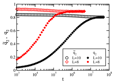
Figure 1: (Color online) Semilog plots of $\widetilde{q}_{2}(t_{0},t)$ and $q_{2}$ vs time $t$ (in MC sweeps) for DIS systems with concentration $x=0.35$ running at the lowest temperature $T_{n}$ for the values of $L$ indicated in the figure. $T=0.075$ ($T=0.05$) for $L=10$ ($L=8$). $q_{2}$ is obtained from averages of $q^{2}$ over time, starting at $t=0$ from an initial random spin configuration. Here, $t_{0}=5\times 10^{7}$ MC sweeps for $L=10$, and $5\times 10^{6}$ MCS for $L=8$. Data points at time $t$ stand for an average over a time interval $[t,1.2t]$, and over $10^{3}$ samples.

In order to check whether this stationary value $q_{2}$ is an equilibrium one, we define a second overlap, $\widetilde{q}_{t}$, not between configurations of pairs of identical replicas at the same time $t$, but between spin configurations of a single replica taken at two different times $t_{0}$ and $t_{1}=t_{0}+t$ of the same MC run,

$$\tilde{q}_{t}(t_{0})=N^{-1}\sum_{j}\sigma_{j}(t_{0})\sigma_{j}(t_{0}+t).$$ (12)

Let $\tilde{q}_{2}(t_{0},t)$ be the average of $(\widetilde{q}_{t}(t_{0}))^{2}$ over all samples. Suppose thermal equilibrium is reached long before time $t_{0}$ has elapsed. Then, $\tilde{q}_{2}(t_{0},t)$ and $q_{2}(t)$ should tend towards a common value $q_{2}$ as $t\rightarrow t_{0}$. Plots of $\tilde{q}_{2}(t_{0},t)$ vs $t$ are shown in Fig. 1 for $t_{0}=5\times 10^{7}$ MC sweeps ($5\times 10^{6}$ MCS sweeps) for $L=10$ ($L=8$) for the same values of $x$ and $T$ as for $q_{2}(t)$. Note that both quantities, $\tilde{q}_{2}(t_{0},t)$ and $q_{2}(t)$, do become approximately equal when $t\rightarrow t_{0}$. In order to obtain equilibrium results, we have always chosen sufficiently large values of $t_{0}$ to make sure that $\tilde{q}_{2}(t_{0},t)\approx q_{2}(t)$ for $t\gtrsim t_{0}$. In our simulations, we let each system equilibrate for a time $t_{0}$ and take averages over the time interval $[t_{0},2t_{0}]$. All values of $t_{0}$ and $N_{s}$ are given in Table II.

It has recently been shown that equilibration times increase with the roughness of the free-energy landscape of each individual sample. yuce2 Numerous spikes in overlap distributions $p_{\cal J}^{~{}Q}$ are the signature of samples that have numerous minima in their free-energy landscape. Visual inspection of overlap distributions of samples like the ones shown in Fig. 2 shows fairly symmetric $p_{\cal J}^{~{}Q}$ curves even though some of them have several spikes. Then, our stringent equilibration criterion suggests that nearly all the samples are well equilibrated.

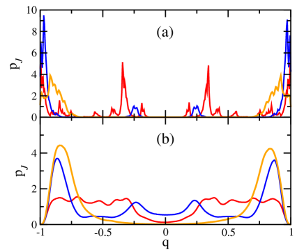
Figure 2: (Color online) (a) Overlap distributions $p_{\cal J}(q)$ for DIS systems with $L=10$, $x=0.35$ and $T=0.1$ for three samples with different realizations of disorder. For each sample we collect values of $q$ over $5\times 10^{7}$ MC sweeps. (b) The same as in (a) but for $T=0.25$ for the same sample set. Recall that the transition temperature is $T_{sg}=0.35$.

III RESULTS

III.1 Overlap distributions

As it has been found for other SG models, it is interesting to examine individual samples of DIS. In Fig. 2(a) we plot $p_{\cal J}(q)$ versus $q$ for different samples at temperature $T/T_{sg}\simeq 0.3$. At this low temperature, some $p_{\cal J}(q)$ display well defined spikes centered on small $q$ values, which seems to vary randomly from sample to sample. Qualitatively similar distributions have been observed for the EA and SK models. yucesoy ; pcf ; aspelmeier It is clear that these inner peaks (that is, peaks away from $q\approx\pm 1$) come from overlaps between states that belong to different basins of attraction. The main aim of this paper is to extract statistical information for these cross-overlap (CO) spikes situated on the interval $q\in(-Q,Q)$. Similar plots for higher temperatures (see Fig. 2(b) for $T/T_{sg}\simeq 0.7$), show that thermal fluctuations render individual spikes not clearly discernible. Then, in order to explore well within the SG phase, we have chosen the lowest temperature in our TMC simulations to be $0.2~{}T_{sg}$. We report most of our results for $T\leq 0.4~{}T_{sg}$. We have also chosen a concentration $x=0.35$ which is far below the threshold for the AF phase. Both low temperatures and low concentrations result in large equilibrium times $t_{0}$. In addition, in order to obtain good sample statistics we need to simulate a large number $N_{s}$ of samples for all system sizes studied. All of this has restricted us to deal with relatively modest system sizes in our simulations. The simulation parameters are given in Tables I and II.

Figure 3(a) shows the sample-averaged overlap distribution $p(q)$ for DIS at $T=0.1$. At this low temperature, $p(q)$ exhibits two large peaks at $\pm q_{m}$ with $q_{m}\approx 1$ and a relatively flat plateau with $p(0)\neq 0$ in the region $q\in(-Q,Q)$ for, say, $Q\approx 1/2$. The non-zero $p(0)$ value does not change with $L$ for the system sizes studied. This behavior, known for the SK and EA models,solutionSK ; kpy is in contradiction with the droplet picture of SGs, for which $p(0)$ vanishes as $L^{-\theta}$.droplet

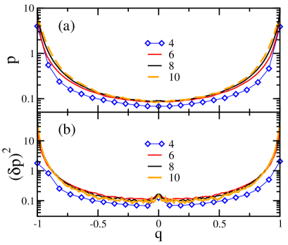
Figure 3: (Color online) (a) Plots of the averaged distribution $p(q)$ versus $q$ for DIS systems with $x=0.35$, $T=0.1$, and the values of $L$ shown. (b) Same as in (a), but for $(\delta p)^{2}$, the mean square deviations of $p_{\cal J}(q)^{2}$ away from $p(q)$ over all $\cal J$ samples.

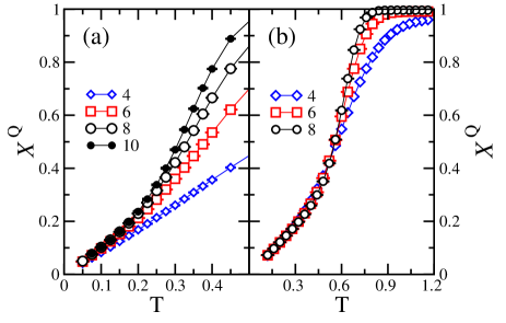
Figure 4: (Color online) (a) Plot of $\it{X}^{Q}$ versus T for DIS systems with $x=0.35$, $Q=1/2$ and the values of $L$ indicated in the figure. (b) The same plots for the SK model, with $Q=1/2$ and the values of $L$ shown. In both panels, error bars are smaller than symbol sizes.

Plots of $(\delta p)^{2}$ vs $p$ are shown for DIS at the same temperature in Fig. 3(b). $\sqrt{(\delta p)^{2}}$, a measure of deviations of $p_{\cal J}(q)$ from the average $p(q)$, is clearly greater than $p$ for $q\in(-1/2,1/2)$ indicating lack of self-averaging. More interestingly, $(\delta p)^{2}$ does not vary appreciably with $L$. This is at odds with the behavior found in MC simulations for the SK model for which $(\delta p)^{2}\propto L$ for $T\leq 0.5~{}T_{sg}$. ourPAD Recall that in the RSB scenario, one expects that $p_{\cal J}(q)$ exhibits with many sharp spikes in the region $q\in(-Q,Q)$ that become $\delta$-like functions as $L$ increases, resulting in a diverging $(\delta p)^{2}$ for macroscopic systems.

III.2 Integrated overlap distributions

Here we consider averages of both $p$ and $(\delta p)^{2}$ over $q\in(-Q,Q)$. This allows us to focus on the contributions of CO spikes and, in addition, to reduce statistical noise if $Q$ is not too small. Plots of $X^{Q}$, the sample-averaged area under CO spikes, versus $T$ are shown for $Q=1/2$ in Figs. 4(a) and 4(b) for DIS and SK models respectively. In both cases, $X^{Q}$ is, as far as we can see, size independent at temperatures well below $T_{sg}$. We obtain quantitatively similar results (not shown) for $Q=1/4$. This is a strong piece of evidence against the validity of the droplet picture, for which $X^{Q}$ is expected to vanish as $TL^{-\theta}$.droplet A similar behavior has been found for the EA model in several MC simulations.kpy ; pcf However, it has been argued that strong finite-size effects may mask the asymptotic behavior at the system sizes currently available to MC simulation.toydroplet Finally, we note that in Figs. 4(a) and (b) $X^{Q}$ seems to vanish as $T\to 0$ (as was long ago predicted for the SK model). vanni

Plots of $\Delta^{Q}$ vs $T$ for DIS in Fig. 5(a) show the presence of finite size effects. Note that for small sizes, $\Delta^{Q}$ increases as $T$ decreases only up to $T=0.15$ ($T=0.075$) for $L=4$ ($L=6$). We return to this point in Section III.3. More interestingly, curves for larger sizes ($L\geq 8$) give a strong indication that $\Delta^{Q}$ does not diverge as $L$ increases. This result is in contradiction with a RSB scenario and is in sharp contrast with the behavior exhibited in Fig. 5(b) for the SK model, for which $\Delta^{Q}$ increases with $\sqrt{L}$ at low temperatures. It is worth mentioning that $\Delta^{Q}$ differs qualitatively from the average $\it{X}_{2}\equiv[~{}(X_{\cal J}^{Q})^{2}~{}]_{\cal J}$ when $Q$ is not very small. pcf $\it{X}_{2}$ has been investigated in detail in several papers and it is known to be size independent for both the EA and SK models. tutti

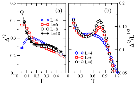
Figure 5: (Color online) (a) Plot of $\Delta_{Q}$ versus T for DIS systems with $x=0.35$, $Q=1/2$ and the values of $L$ indicated in the figure. (b) Plot of $\Delta_{Q}/L^{1/2}$ versus $T$ for the SK model, with $Q=1/2$.

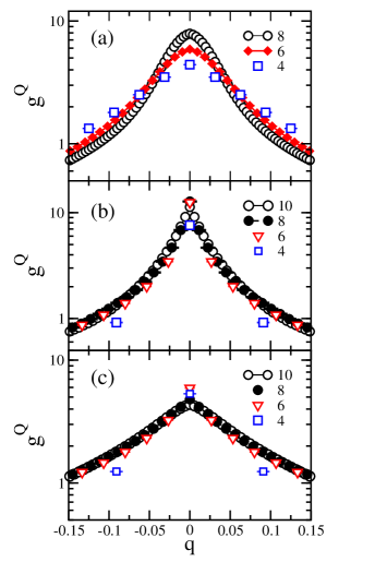
Figure 6: (Color online): (a) Plots of $g^{Q}$ vs $q$ for the SK model at $T=0.2$ with $Q=1/2$ and the values of $L$ shown. (b) Same plot as for (a) but for DIS systems with $x=0.35$ at $T=0.075$. (c) Same plot as for (b) but for $T=0.125$.

III.3 Pair correlation functions

Data points for the pair correlation function $g^{Q}$ for $Q=1/2$ are shown in Fig.6(a) and (b) for the SK model at $T=0.2$ and DIS at $T=0.075$ respectively. Note that these temperatures are such as $T/T_{sg}\simeq 0.2$ in both cases. We find curves that are rather pointed with widths clearly smaller than $Q$. We obtain similar results for $Q=1/4$. Data for DIS in Fig. 6(b) do not exhibit any significant size dependence. In contrast, $g^{Q}$ curves for SK in Fig. 6(a) become sharper as $L$ increases. This result for the SK model is as expected for a RSB scenario. In the RSB solution, $p_{\cal J}(q)$ is made of several cross-overlap spikes that for small values of $q$ become $\delta$-functions in the macroscopic limit, and densely fill the interval $q\in(-Q,Q)$. In striking contrast, our result for DIS suggest that the number of SG states do not grow with $L$ at finite low temperatures.

Some people have argued that comparing data for different models (EA and SK) at the same value of $T/T_{sg}$ is not meaningful. They find more appropriate to make such a comparison at temperatures for which $X^{Q}$ values are the same.critico We follow this recipe and compare the data shown in Fig. 6(c) for DIS at $T=0.125$ and in Fig. 6(a) for the SK model at $T=0.2$. Apart from the fact that $g^{Q}$ becomes narrower as $T$ decreases, we do not notice any qualitative difference.

It is interesting to note that spikes, even though they have non-zero widths $w$ at finite $T$, may not be discerned in $p_{\cal J}(q)$ distributions of very small systems. Note that the minimum appreciable value of $q$ for systems of $N$ spins is given by $\Delta q=2/N$. Thus, finite size effects are expected to come at very low $T$ when $w\lesssim\Delta q$. This seems to be the case for the data shown in Figs. 5(a) and 7(a) for $L=4$ ($L=6$) and $T\lesssim 0.15$ ($T\lesssim 0.075$).

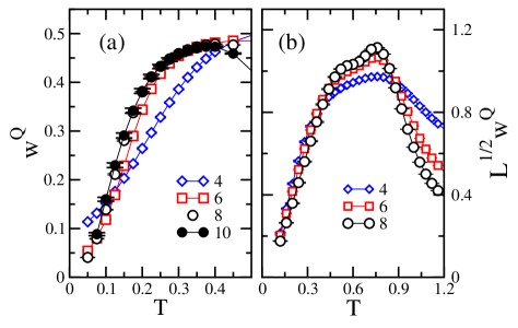
Figure 7: (Color online) (a) Plots of $w{Q}$ vs $q$ for DIS systems with $x=0.35$ for $Q=1/2$ and the values of $L$ shown. (b) Plots of $L^{1/2}w{Q}$ vs $q$ for (a) but for the SK model, $Q=1/2$ and the values of $L$ shown. In both panels all error bars are smaller than symbol sizes.

Plots of $w^{Q}$ versus $T$ are shown in Figs. 7(a) and  7(b) for DIS and the SK model respectively. $w^{Q}$ appear in Fig. 7(a) to be size independent at least for $L\geq 8$. This points to finite widths for CO spikes in the $L\rightarrow\infty$ limit for low (but finite) temperature. On the other hand $w^{Q}$ values for the SK model displayed in Fig. 7(b) appear to vanish as $1/L^{1/2}$ as $L$ increases at least for $T\lesssim 0.4$, in agreement with the RSB picture.

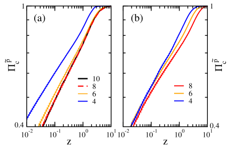
Figure 8: (Color online) (a) Plot of the cumulative distribution $\Pi\{\widetilde{p}^{~{}Q}_{\cal J}\}$ versus $x$ for DIS systems with $x=0.35$, for $Q=1/2$, $T=0.1$ and the values of $L$ indicated in the figure, where $\widetilde{p}^{Q}_{\cal J}$ is the maximum value of $p_{\cal J}(q)$ over the interval $-Q\leq q\leq Q$. (b) The same plot as in (a) but for the SK model, for $Q=1/2$, $T=0.16$ and the values of $L$ shown.

III.4 Cumulative distributions

As interesting as they could be, pair correlation functions (PCFs) do only give information on how spiky sample distributions $p_{\cal J}(q)$ are in the $(-Q,Q)$ region. However, PCFs do not give any information about the height of spikes located there. Following seminal work by Yucesoy et al. yucesoy we study here $\Pi_{c}^{\widetilde{p}}(z)$, the fraction of samples without any spike in $(-Q,Q)$ with height larger than $z$. Plots of $\Pi_{c}^{\widetilde{p}}$ versus $z$ for DIS at $T=0.1$ are shown in Fig. 8(a). They give a strong indication that $\Pi_{c}^{\widetilde{p}}$ reach a size-independent shape for $L\geq 8$ for a wide range of values of $z$. In order to check for the robustness of our $\Pi_{c}^{\widetilde{p}}(z)$ values, we have grouped all available samples in $K$ ensembles of $10^{3}$ samples each, calculated $\Pi_{c}^{\widetilde{p}}$ for each ensemble $k=1,...,K$, and obtained the standard deviation (SD) of the $K$ resulting values. Tiny vertical bars in Figs. 8 and 9 stand for such SDs. Plots in Fig. 8(a) are to be compared with the ones displayed in Fig. 8(b) for the SK model. Note in Fig. 8(b) that, at least for $z\gtrsim 0.5$, $\Pi_{c}^{\widetilde{p}}(z)$ clearly decreases as $L$ increases, indicating a proliferation of high spikes for larger sizes. This is as expected for the RSB picture, for which CO spikes become $\delta$-like functions in the thermodynamic limit.

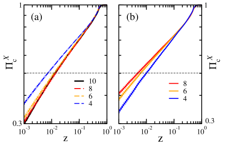
Figure 9: (Color online) (a) Plot of the cumulative distribution $\Pi\{X^{Q}_{\cal J}\}$ versus x for DIS systems with $x=0.35$, for $T=0.1$ and the values of $L$ indicated in the figure. (b) The same plots as in (a) but for the SK model, for $T=0.16$.

Finally, we report results on how the random variable $\it{X}_{\cal J}^{Q}$ is distributed. Previous MC simulations have found a similar behavior for the EA and SK models when dealing with the cumulative distribution $\Pi_{c}^{\it X}(z)$ of quantity $z=\it{X}_{\cal J}^{Q}$. yucesoy ; billoire The mean-field theory of the SK model offers precise predictions on $\Pi_{c}^{\it X}(z)$ and their moments. tutti In particular, $\Pi_{c}^{\it X}(z)$ is found to follow a power law for small $z$. For small values of $Q$,mezard $\Pi_{c}^{\it X}(z)\propto z^{\it y}$, where $\it y$ stands here for $\it{X}^{Q}$. Some people have found it useful to study the median of the cumulative distribution, which is predicted to reach a non-zero value in the thermodynamic limit in the RSB picture but vanishes for the droplet model. Log-log plots of $\Pi_{c}^{\it X}$ versus $X$ for DIS displayed in Fig. 9(a) show curves with power-law behavior for small $z$. Data do not show any significant deviation for sizes $L\geq 8$. The median (marked by the crossings points of the curves with the horizontal dotted line in the figure) decreases as $L$ increases reaching a non-zero value. The counterpart plots for the SK model are shown in Fig. 9(b). In agreement with previous MC work on the SK model, billoire ; wittmann we find strong finite-size effects. However, curves seem to converge to some limiting curve as $L$ increases.billoire Note that, in contrast with DIS, the median of $\Pi_{c}^{\it X}$ increases as $L$ increases. All our results for $\Pi_{c}^{\it X}$ for both the SK model and DIS are not in contradiction with a RSB scenario.

IV Conclusions and discussion

By tempered Monte Carlo calculations, we have studied the low temperature behavior of a diluted system of classical dipoles placed on a SC lattice. These dipoles are Ising spins randomly placed on a fraction $x$ of all lattice sites and point up or down along a common crystalline axis.

Previous MC studies pcf for this model have provided strong evidence for the existence of a SG phase for $x\lesssim 0.65$ with a SG transition temperature $T_{sg}(x)\simeq x$. The SG phase was then found to have quasi-long range order, as in the 2D-XY model. xy Neither the droplet model nor a RSB scenario fit with this marginal behavior. Despite the existence of this soft SG order, we find in our simulations spiky overlap distributions $p_{\cal J}(q)$ that are strongly sample-dependent, as previously found in simulations for the EA and the SK models.yucesoy ; pcf ; aspelmeier

We have studied the statistics of $p_{\cal J}(q)$ for $q\in(-Q,Q)$ using some recently proposed observables. yucesoy ; pcf ; billoire We find that $p(q)$ and $\delta p(q)$ (as well as their integrated counterparts $X^{Q}$ and $\Delta^{Q}$) do not vary appreciably with $L$.

From a suitable defined pair correlation function pcf we compute an averaged width $w^{Q}$ that appears to remain finite as $L$ increases. Complementary to this result, we find that the fraction of samples with spikes higher than a certain threshold does not vary appreciably with $L$. All of this points to finite width for CO spikes in the $L\to\infty$ limit at low temperatures.

Our results are in clear contradiction with droplet model predictions. On the other hand, a direct comparison of our data with MC data obtained for the SK model shows that crucial RSB predictions are also at odds with some of our results. It is noteworthy that the findings enumerated above for DIS are strikingly similar to the ones found in previous MC work for the EA model, yucesoy ; pcf ; billoire ; wittmann though finite size effects have been reported to be strong for the EA model for the available systems sizes in MC simulations.

References

- (1) S. E. Page, Diversity and Complexity, (Princeton University Press, Princeton, NJ, 2010); S. Lloyd, IEEE Control Syst. Mag. 21, 7 (2001); R. N. Mantegna and H. E. Stanley, An Introduction to Econophysics: Correlations and Complexity in Finance (Cambridge University Press, Cambridge, UK, 2000).
- (2) G. Parisi, arXiv:cond-mat/9412018v1 (1994); T. Aspelmeier, A. J. Bray, and M A Moore, Phys. Rev. Lett. 92, 087203 (2004).
- (3) D. Sherrington and S. Kirkpatrick, Phys. Rev. Lett. 32, 1792 (1975); S. Kirkpatrick and D. Sherrington, Phys. Rev. B 17, 4384 (1978).
- (4) G. Toulouse, Commun. Phys. 2, 115 (1977).
- (5) D. L. Stein and C. M. Newman, Spin Glasses and Complexity (Princeton University Press, Princeton, NJ, 2012).
- (6) M. Mézard, G. Parisi, and M. Virasoro, Spin Glass Theory and Beyond (World Scientific, Singapore, 2004).
- (7) J. Thouless, P. W. Anderson, and R. Palmer, Philos. Mag. 35, 593 (1977); A. J. Bray and M. A. Moore, Phys. Rev. Lett. 41, 1068 (1978).
- (8) G. Parisi, Phys. Rev. Lett. 43, 1754 (1979); ibid 50, 1946 (1983); for a review, see E. Marinari, G. Parisi, and J. J. Ruiz-Lorenzo, in Spin Glasses, edited by K. H. Fischer and J. A. Hertz, (Cambridge University Press, Cambridge, 1991); E. Marinari, G. Parisi, F. Ricci-Tersenghi, J. J. Ruiz-Lorenzo, and F. Zuliani, J. Stat. Phys 98, 973 (2000).
- (9) K. Binder and A. P. Young, Rev. Mod. Phys. 58, 801 (1986).
- (10) S. F. Edwards and P. W. Anderson, J. Phys. F, 5, 965 (1975).
- (11) R. N. Bhatt and A. P. Young, Phys. Rev. Lett. 54, 924 (1985); A. T. Ogielski and I. Morgenstern, Phys. Rev. Lett. 54, 928 (1985); R. N. Bhatt and A. P. Young, Phys. Rev. B 37, 5606 (1988).
- (12) C. M. Newman and D. L. Stein, Phys. Rev. E 57, 1356 (1998); C. M. Newman and D. L. Stein, Phys. Rev. Lett. 76, 4821 (1996).
- (13) D. S. Fisher and D. A. Huse, J. Phys. A 20, L1005 (1987); D. S. Fisher and D. A. Huse, Phys. Rev. B 38, 386 (1988); M. A. Moore, H. Bokil, and B. Drossel, Phys. Rev. Lett. 81, 4252 (1998); M. A. Moore, J. Phys A 38, L783 (2006).
- (14) F. Krzakala and O. C. Martin, Phys. Rev. Lett. 85, 3013 (2000); M. Palassini and A. P. Young, Phys. Rev. Lett. 85, 3017 (2000).
- (15) H. G. Katzgraber, M. Palassini, and A. P. Young, Phys. Rev. B 63, 184422 (2001).
- (16) A. A. Middleton, Phys. Rev. B 87, 220201 (2013).
- (17) R. A. Baños, A. Cruz, L. A. Fernandez, J. M. Gil-Narvion, A. Gordillo-Guerrero, M. Guidetti, D. Iñiguez, A. Maiorano, F. Mantovani, E. Marinari, V. Martin-Mayor, J. Monforte-Garcia, A. Muñoz Sudupe, D. Navarro, G. Parisi, S. Perez-Gaviro, F. Ricci-Tersengui, J. J. Ruiz-Lorenzo, S. F. Schifano, B. Seoane, A. Tarancón, R. Tripiccione, and D. Yllanes, Phys. Rev. B 84, 174209 (2011).
- (18) B. Yucesoy, H. G. Katzgraber, and J. Machta, Phys. Rev. Lett. 109, 177204 (2012).
- (19) J. F. Fernández and J. J. Alonso, Phys. Rev. B 86, 140402R (2012); J. F. Fernández and J. J. Alonso, Phys. Rev. B 87, 134205 (2013).
- (20) A. Billoire, A. Maiorano, E. Marinari, V. Martin-Mayor, and D. Yllanes, Phys. Rev. B 90, 094201 (2014).
- (21) A. Billoire, L. A. Fernandez, A. Maiorano, E. Marinari, V. Martin-Mayor, G. Parisi, F. Ricci-Tersenghi, J. J. Ruiz-Lorenzo, and D. Yllanes, Phys. Rev. Lett. 110, 219701 (2013).
- (22) Creighton K. Thomas, David A. Huse, and A. A. Middleton, Phys. Rev. Lett. 107, 047203 (2011).
- (23) M. Wittmann, B. Yucesoy, H. G. Katzgraber, J. Machta, and A. P. Young Phys. Rev. B 90, 134419 (2014).
- (24) C. Wengel, C. L. Henley, and A. Zippelius, Phys.Rev. B 53, 6543 (1996).
- (25) J. Luttinger and L. Tisza, Phys. Rev. B 72, 257 (1947).
- (26) J. F. Fernández and J. J. Alonso, Phys. Rev. B 62, 53 (2000).
- (27) W. Luo, S. R. Nagel, T. F. Rosenbaum, and R. E. Rosensweig, Phys.Rev. Lett. 67, 2721 (1991).
- (28) A. H. Cooke, D. A. Jones, J. F. A. Silva, and M. R. Wells, J. Phys. C: Solid State Physics 8, 4083 (1975).
- (29) J.Villain, Z. Physik B 33, 31 (1979).
- (30) D. H. Reich, B. Ellman, J. Yang, T. F. Rosenbaum, G. Aeppli, and D. P. Belanger, Phys. Rev. B 42, 4631 (1990); W. Wu, D. Bitko, T. F. Rosenbaum, and G. Aeppli, Phys. Rev. Lett. 71, 1919 (1993); C. Ancona-Torres, D. M. Silevitch, G. Aeppli, and T. F. Rosenbaum, Phys. Rev. Lett. 101, 057201 (2008).
- (31) K. M. Tam, and M. J. P. Gingras, Phys.Rev. Lett. 103, 087202 (2009).
- (32) J. C. Andresen, H. G. Katzgraber, V. Oganesyan, and M. Schechter, Phys. Rev. X 4, 041016 (2014) .
- (33) J. J. Alonso, and J. F. Fernández, Phys. Rev. B 81, 064408 (2010).
- (34) M. Palassini and S. Caracciolo, Phys. Rev. Lett. 82, 5128 (1999).
- (35) E. Marinari and G. Parisi, Europhys. Lett. 19, 451 (1992); K. Hukushima and K. Nemoto, J. Phys. Soc. Jpn. 65, 1604 (1996).
- (36) J. F. Fernández, Phys. Rev. B 78, 064404 (2008); J. F. Fernández and J. J. Alonso, Phys. Rev. B 79, 214424 (2009).
- (37) N. A. Metropolis, A. W. Rosenbluth, M. N. Rosenbluth, A. H. Teller, and E. Teller, J. Chem. Phys 21, 1087 (1953).
- (38) B. Yucesoy, J. Machta and H. G. Katzgraber, Phys. Rev. E 87, 012104 (2013).
- (39) T. Aspelmeier, A. Billoire, E. Marinari, and M. A. Moore, J. Phys. A 41, 324008 (2008).
- (40) J. Vannimenus, G. Toulouse, and G. Parisi, J. Phys. (Paris) 42, 565 (1981).
- (41) M. Mézard, G. Parisi, N. Sourlas, G. Toulouse, and M. Virasoro, Phys. Rev. Lett. 52, 1156 (1984).
- (42) J. M. Kosterlitz and D. J. Thouless, J. Phys.C 6, 1181 (1973); J. M. Kosterlitz, ibid. 7, 1046 (1974); see also, J. V. José, L. P. Kadanoff, S. Kirkpatrick, and D. R. Nelson, Phys. Rev. B 16, 1217 (1977); J. Villain, J. Phys. (Paris) 36, 581 (1975); J. F. Fernández, M. F. Ferreira, and J. Stankiewicz, Phys. Rev. B 34, 292-300 (1986); H. G. Evertz and D. P. Landau, Phys. Rev. B 54, 12302 (1996).