Time-delayed intensity-interferometry of the emission from ultracold atoms in a steady-state magneto-optical trap

Abstract

An accurate measurement of the bunching of photons in the fluorescent emission from an ultracold ensemble of thermal ${}^{87}Rb$ atoms in a steady-state magneto-optical trap is presented. Time-delayed-intensity-interferometry (TDII) performed with a 5-nanosecond time resolution yielded a second-order intensity correlation function that has the ideal value of 2 at zero delay, and that shows coherent Rabi oscillations of upto 5 full periods - much longer than the spontaneous emission lifetime of the excited state of Rb. The oscillations are damped out by $\sim 150$ns, and thereafter, as expected from a thermal source, an exponential decay is observed, enabling the determination of the temperature of the atomic ensemble. Values so obtained compare well with those determined by standard techniques. TDII thus enables a quantitative study of the coherent and incoherent dynamics, even of a large thermal ensemble of atomic emitters.

Intensity interferometry, or the measurement of photon correlation, provides a wealth of information regarding the light source and the mechanism of emission. A study of the mere arrival times of photons from the source enables one to determine its nature - whether it is thermal (chaotic), or coherent, or quantum. The form of approach to the asymptotic value allows one to infer further details of the source. For example, one of the earliest measurements HBT of spatial photon correlation of light from the star Sirius enabled the determination of the diameter of the star. Intensity interferometry is routinely used in particle physics Baym ; particle-physics to study decay processes and to deduce the interaction between particles. Other applications include the search for naturally occuring non-classical sources of radiation in astrophysics stellar , study of light emission from nanostructures Bayer and particle size measurements DLS . Typically, pairs of detectors either seek the simultaneous arrival of photons, or measure the delayed arrival of a photon at one detector with respect to the arrival of a photon at the other. The measurements are quantified by the second order correlation function, (also known as intensity-intensity correlation function), $g^{(2)}(R,\tau)=\frac{\Big{\langle I_{1}(r,t)\Big{\rangle}\Big{\langle}I_{2}(r+R,t+\tau)\Big{\rangle}}}{\Big{\langle I_{1}(r,t)\Big{\rangle}\Big{\langle}I_{2}(r,t)\Big{\rangle}}}$, where $I_{1}(r,t)$ and $I_{2}(r+R,t+\tau)$ are the intensities of light reaching detectors D1 and D2 at locations r and r+R at times $t$ and $t+\tau$ and the angular brackets denote time averaging. It is the correlation of the number of photons, or intensities, that is examined, as opposed to a correlation of amplitudes in conventional interferometers, and hence the name time-delayed intensity-interferometry (TDII). It has been theoretically shown that (see, for example Baym ) that the second order correlation function $g^{(2)}(\tau=0)$ = 2 for a thermal state, implying a tendency for bunched or correlated emission of photons; is unity for a coherent source, implying emission of photons at random times, and equals $1-\frac{1}{n}$ for a n-photon Fock state, signifying anti-bunching. The value of $g^{(2)}(\tau)\,\,$for all sources, however, approaches unity for long time delays.
Temporal bunching of photons from thermal sources, ever since the postulation of the concept, has been an intriguing phenomenon, and has been the focus of numerous experiments. The earliest laboratory thermal source studied was a Hg vapour lamp Hg1 , light from which showed a meagre bunching of 1.17. Martiensen and Spiller devised a method of creating pseudo-thermal light by transmitting coherent laser light through a rotating ground glass plate GroundGlass such that the time-varying surface inhomogenieties introduced temporal and spatial decoherence. In recent years, laboratory control and measurement techniques have enabled creation of pseudo-thermal light sources with theoretically expected values of $g^{(2)}(\tau)\,\,$= 2 Anders ; AB-EPL ; JOSA ; EPJP .
We report here Time-Delayed Intensity-Interferometric measurements on light from another source of bunched photons - an ensemble of laser cooled atoms. Though laser cooled atoms have been available for more than three decades, direct TDII measurements of their emission have been very fewAspect ; Bali ; Nakayama . All measurements hitherto have been carried out in optical molasses, which were either periodically, or continuously loaded with atoms precooled in a MOT. In this paper we present measurements of the second order correlation function of light emitted by ultracold atoms in a steady-state magneto-optical trap, where the cooling and repumper beams, and also the quadrupolar magnetic field are kept on. We observe the ideal value of 2 for the zero-delay intensity-intensity correlation function. Damped Rabi oscillations are observed for time delays upto $\sim 150$ns, and an exponential decay for longer time delays. Despite the fact that the emission being studied is from a collection of uncorrelated atoms that are in random thermal motion, and that the observations are averaged over an 8-hour period, coherent effects are seen, bringing out the power of higher order correlations in revealing hidden periodicities and providing a measure of coherent and incoherent dynamics. The exponential decay at long time delays was used to determine the temperature of the ensemble.
Time delayed Intensity Interferometry was performed on the fluorescent emission from ⁸⁷Rb atoms cooled and trapped in a magneto-optical trap (MOT) (Fig. 1), which differed from usual MOTs, in that the two pairs of beams in the x-y plane were steeply inclined to each other, enclosing an angle of 55^∘ rather than the usual 90^∘ so as to accomodate, within the chamber, a pair of lenses of short-focal length and high numerical aperture. These lenses were positioned facing each other, such that their focal points coincided with the centre of the MOT and could thus be used to focus light onto the MOT, or collect light emitted by a small volume within the cold cloud. To avoid clipping at the lens mounts leading to undesired scattered light, the diameters of the beams in the x-y plane were restricted to $\sim$1.5mm while the z-beam had a diameter of 8mm. The cooled and trapped atoms were viewed using a CCD camera, and their number estimated by collecting part of the fluorescent light onto a femtowatt detector. The typical cloud was roughly ellipsoidal with a mean diameter of $\sim 400\mu$m, and contained about 20000 atoms.

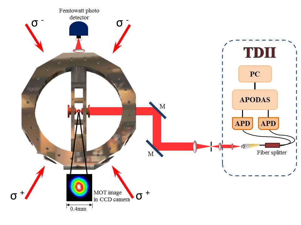
Figure 1: Schematic of the experiment showing the collection of cold atoms inside the MOT chamber. A lens within the chamber collects fluorescence from the atoms, which is passed onto the TDII setup where the arrival of individual photons are time-stamped and archived. Bold arrows show the cooling beams in the x-y plane. The z-beams (perpendicular to the page) are not shown.

An intensity-interferometer was formed using a fiber splitter, where the two output ends were connected to two high speed APDs that had quantum efficiencies of 65$\%$ and a dead time of 30ns. The output of the APDs were fed to a homebuilt, FPGA-based time-tagged-single-photon recorder, APODAS (Avalanche Photodiode Optical Data Acquisition System arXiv that utilised high speed ethernet connectivity and stored, in a PC in realtime, the arrival times of all detected photons with a temporal resolution of 5 nanoseconds. Post-processing by software enabled the determination of $g^{(2)}(\tau)\,\,$for all $\tau$ from a single recording of the data EPJP . As we worked in the photon-counting mode, the expression for $g^{(2)}(\tau)\,\,$in terms of coincidences is Bali

$$g^{(2)}(\tau)=N_{c}T/(N_{1}N_{2}\tau_{c})$$ (1)

where $\tau$ at is the delay between arrival at the two detectors, $N_{1},N_{2}$ and $N_{c}$ are the number of counts at detector 1, detector 2 and the coincident counts respectively. T is the total observation time and $\tau_{c}$ the time window for coincidence (arrival of two photons is considered simultaneous if they are detected within a time gap of $\tau_{c}$).

For determining the bunching characteristics of emission from an ultracold atomic ensemble, ⁸⁷Rb atoms were laser cooled from close to room temperature, to $\sim 100\mu$K. The MOT was extremely stable, with the lasers locked and the cold cloud in steady-state for days. A typical run of the experiment lasted 8 hours. The cold cloud was obtained, and the cooling and repumper beams, and the magnetic field were kept switched on for the entire duration of the experiment. The cold ensemble was constantly monitored by imaging it on a camera, and also by measuring the fluorescence on a femtowatt detector (see Fig. 1). For the purpose of determining its second order correlation function, fluorescence light from the central region of the cloud was collected by the high-numerical aperture lens placed inside the sample chamber, a few millimeters from the trap centre. Care was taken to ensure that no part of the laser light entered this lens, either directly, or upon being scattered by the parts of the MOT chamber. The light was conveyed by a series of mirrors and lenses to the input of the TDII setup. The count registered in the presence of the cold cloud was in the range 40,000 - 80,000/s while in the absence of the cold cloud it reduced to $\sim$1200/s, confirming that it is predominantly light from the cold atoms that enters the TDII setup. Photon arrival time data was recorded for various detunings of the cooling beam. For each detuning the number of atoms trapped was estimated from the fluorescent intensity recorded on the femtowatt detector. While the total number of atoms collected ranged from $\sim 8000$ to $\sim 22000$, the high numerical aperture lens employed for accepting light for TDII measurement restricted the collection of light to that from approximately one-tenth of the volume of the cold ensemble. The temperature of the collection of atoms was determined by the trap oscillation method trap-osc , and was found to range from $200\mu$K to $50\mu$K for detunings of the cooling laser varying from -12MHz to -22MHz. The effective Rabi frequencies ranged from 25MHz to 40MHz.

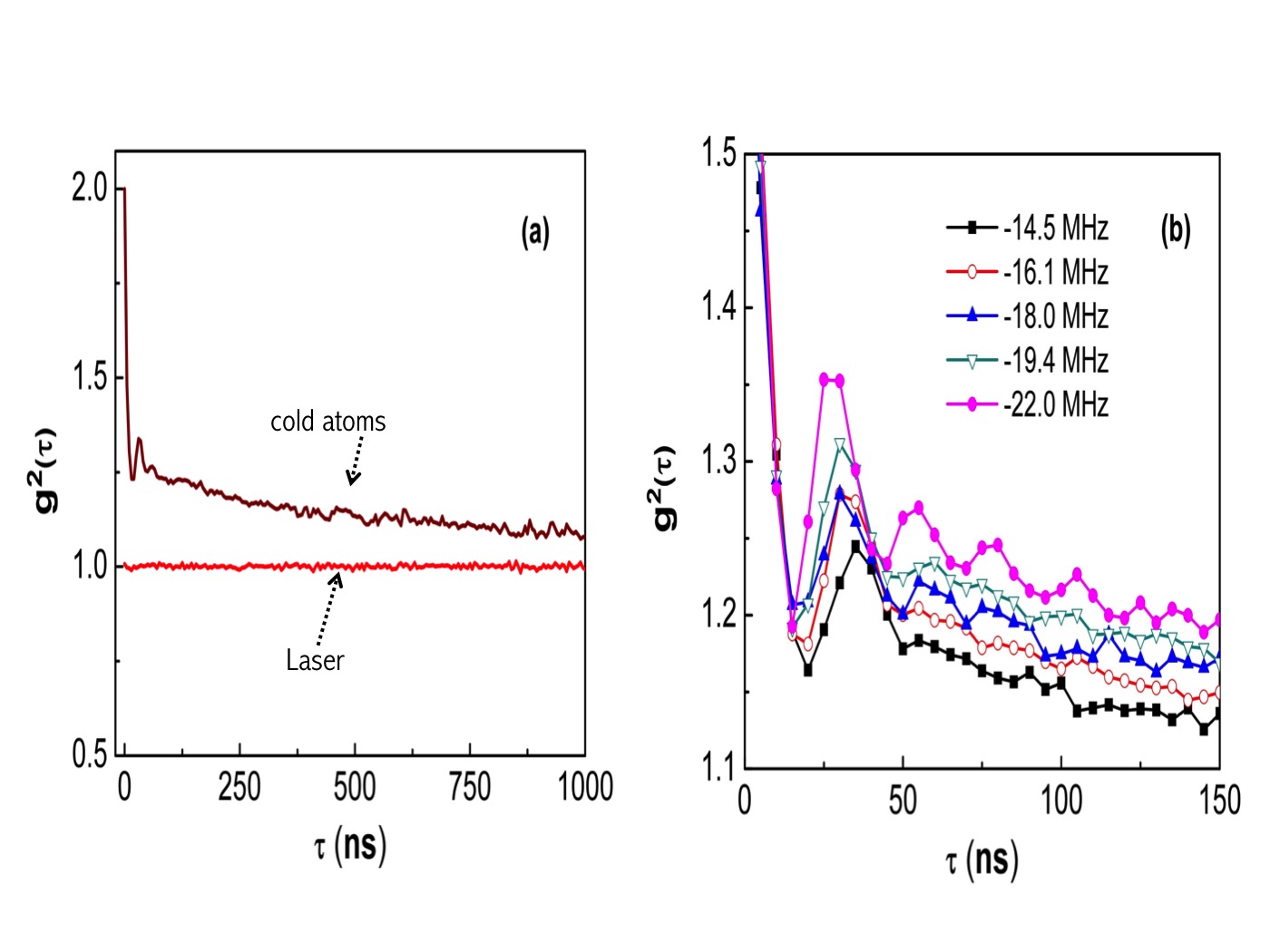
Figure 2: (a) Experimentally obtained $g^{(2)}(\tau)$ vs $\tau$ for laser light measured before its entry to the MOT chamber (red) and for fluorescence light from the cold atoms (brown), and (b) Oscillations seen $g^{(2)}(\tau)\,\,$at short time scales, for different detunings of the cooling beams; the curves are drawn as a guide to the eye, and the values of the detuning are given in the legend.

Two-time intensity-correlation values were derived from the TDII measurements. Fig. 2a shows the second order correlation functions of the input laser light determined before it enters the MOT chamber, and of the light emitted by the ultracold atoms trapped in the MOT. It is clear that absorption and re-emission by the thermal ensemble of atoms has led to bunching in light, which was initally coherent ($g^{(2)}(\tau)\,\,$= 1 for all $\tau$). Several interesting features are observed in $g^{(2)}(\tau)\,\,$for light from the cold atoms. Periodic oscillations, are seen; these are damped out by $\sim 150$ns, and thereafter the curve decays steadily towards unit value. The curve $g^{(2)}(\tau)\,\,$is less noisy for small $\tau$ than for larger ones. As the cooling beams are further detuned from the $5S_{1/2}F=2\rightarrow 5P_{3/2}F=3$ transition (the so-called ”cooling transition”), the value of $g^{(2)}(0)\,\,$approaches closer to 2 while the oscillations in correlation are more prominent and more rapid, and their damping is slower (Fig. 2b).
Let us, for simplicity, assume the Rb atom to be a 2- level system. Irradiation of an atom by coherent, near resonant light causes two processes to occur. One is the periodic absorption and coherent emission of radiation leading to an oscillation between the excited and the ground state at the Rabi frequency - a rate determined by the intensity and detuning of the incoming radiation. The other is the absorption and spontaneous random emission, at a rate that falls exponentially with a characteristic lifetime, which, for the excited state of ⁸⁷Rb is $\sim$28ns. The atoms in the ensemble, being uncorrelated, do not emit in unison, and thus no periodicity will be evident in the direct observation of emission from the collection. However, all atoms undergo Rabi oscillations at the same frequency, and thus have a high probability of emission at the same regular interval. The second order correlation, which is a measure of the probability of emission at time $t+\tau$ conditioned on an emission having occurred at time $t$, will therefore exhibit periodic maxima at regular intervals $\tau_{R}$, the inverse of the Rabi frequency. Thus, the two-time intensity correlation measurement is a simple yet powerful technique that can reveal hidden periodicities. The periodic oscillations arising from coherent dynamics under steady-state driving fields, nevertheless, show decay as decoherence sets in due to spontaneous emission and inter-atomic collisions. This reasoning also explains why $g^{(2)}(\tau)\,\,$is less noisy for short time delays than for larger delays. The Rabi frequency in our experiment being a few tens of MHz, coherent oscillations should occur at the time scales of few tens of nanoseconds. The lifetime of the excited state is $\sim 28$ns, implying that a decay in amplitude of oscillation will occur over $\sim 100$ns ( a few lifetimes). Interatomic collisions occur at yet longer time scales. Thus, short delays show cleaner curves.
Let us consider a thermal collection of $N$ independent atoms under the action of a near-resonant driving field of Rabi frequency $\Omega$. The electric field ${\mathcal{E}}(\vec{r})$ due to coherent emission, at a point of observation $\vec{r}$ is the resultant of contributions from each atom, $j$, and may be written as (Eq. 13.48 in GSA )

$${\mathcal{E}}(\vec{r})\,\,\,\,=\,\,\,\,\displaystyle\sum_{j=1}^{N}{\mathcal{E}_{j}}\,\,\,\,\sim\,\,\,\,\displaystyle\sum_{j=1}^{N}K_{j}{S_{j}}(e\rightarrow g)e^{i\phi_{j}}$$ (2)

where $S_{j}(e\rightarrow g)$, is the de-excitation operator for the two-level atom, the dynamics of which is given by the master equation for the driven two-level atom (Eq. 13.1 in GSA ), and $\phi_{j}$ the phase of the electric vector (due to the coherent emission of the $j^{th}$ atom) at the point of observation (detection) depends on the location of the atom and the orientation of the atomic dipole. In a MOT, the resultant driving field due to the six cooling beams varies in a complex manner in intensity and polarization from position to position. Likewise, the orientation of each atom varies as it moves within the MOT region (see for example Gomer ).
The second order intensity correlation function is defined as :

$$g^{(2)}(\tau)=\frac{\langle\mathcal{E}^{\dagger}(0)\mathcal{E}^{\dagger}(\tau)\mathcal{E}(\tau)\mathcal{E}(0)\rangle}{\langle\mathcal{E}^{\dagger}(0)\mathcal{E}(0)\rangle^{2}}$$ (3)

Substituting from Eq.2 to Eq.3 yields terms of the following forms, with appropriate prefactors :

$$(a)\hskip 14.22636pt\displaystyle\sum_{j=1}^{N}\langle\mathcal{E}_{j}^{\dagger}(0)\mathcal{E}_{j}^{\dagger}(\tau)\mathcal{E}_{j}(\tau)\mathcal{E}_{j}(0)\rangle$$

$$(b)\hskip 14.22636pt\displaystyle\sum_{i=1}^{N}\displaystyle\sum_{j=1,j\neq i}^{N}\langle\mathcal{E}_{i}^{\dagger}(0)\mathcal{E}_{j}^{\dagger}(\tau)\mathcal{E}_{j}(\tau)\mathcal{E}_{i}(0)\rangle$$

$$(c)\hskip 14.22636pt\displaystyle\sum_{i=1}^{N}\displaystyle\sum_{j=1,j\neq i}^{N}\langle\mathcal{E}_{i}^{\dagger}(0)\mathcal{E}_{j}^{\dagger}(\tau)\mathcal{E}_{i}(\tau)\mathcal{E}_{j}(0)\rangle$$

$$(d)\hskip 14.22636pt\displaystyle\sum_{i=1}^{N}\displaystyle\sum_{j=1,j\neq i}^{N}\langle\mathcal{E}_{i}^{\dagger}(0)\mathcal{E}_{i}^{\dagger}(\tau)\mathcal{E}_{j}(\tau)\mathcal{E}_{j}(0)\rangle$$

$$(e)\hskip 14.22636pt\displaystyle\sum_{i=1}^{N}\displaystyle\sum_{j=1,j\neq i}^{N}\displaystyle\sum_{k=1,k\neq i,j}^{N}\langle\mathcal{E}_{i}^{\dagger}(0)\mathcal{E}_{j}^{\dagger}(\tau)\mathcal{E}_{k}(\tau)\mathcal{E}_{i}(0)\rangle\text{\,\,and various permutations }$$

$$(f)\hskip 14.22636pt\displaystyle\sum_{i=1}^{N}\displaystyle\sum_{j=1,j\neq i}^{N}\displaystyle\sum_{k=1,k\neq i,j}^{N}\displaystyle\sum_{l=1,l\neq i,j,k}^{N}\langle\mathcal{E}_{i}^{\dagger}(0)\mathcal{E}_{j}^{\dagger}(\tau)\mathcal{E}_{k}(\tau)\mathcal{E}_{l}(0)\rangle$$

Terms of the form (a) represent single-atom contributions. At $\tau=0$ these show antibunching - an atom cannot emit more than one photon at a time.
Recognising that the emitters are a thermal collection of uncorrelated atoms, the operators in the terms in (b) may be re-ordered and factorised to yield :

$$(b) \triangleq\displaystyle\sum_{i=1}^{N}\displaystyle\sum_{j=1,j\neq i}^{N}[\langle\mathcal{E}_{i}^{\dagger}(0)\mathcal{E}_{i}(0)\rangle\langle\mathcal{E}_{j}^{\dagger}(\tau)\mathcal{E}_{j}(\tau)\rangle]$$

$$=N(N-1)\frac{I^{2}}{N^{2}}$$

where $I$ is the total intensity at the detector due to $N$ atoms. On similar lines, terms in (c) lead to the auto-correlation :

$$(c) \triangleq N(N-1)|\langle\mathcal{E}_{j}^{\dagger}(\tau)\mathcal{E}_{j}(0)\rangle|^{2}$$

Terms consituting (d) are related to the anomalous correlation, which, for a thermal cloud, vanish on time averaging. Similarly, terms (e) and (f), due to the random phases, also drop out upon time averaging. From these arguments, we now find that

$$\langle\mathcal{E}^{\dagger}(0)\mathcal{E}^{\dagger}(\tau)\mathcal{E}(\tau)\mathcal{E}(0)\rangle =N[\langle\mathcal{E}_{j}^{\dagger}(0)\mathcal{E}_{j}^{\dagger}(\tau)\mathcal{E}_{j}(\tau)\mathcal{E}_{j}(0)\rangle]\,\,\,+\,\,\,N(N-1)\Big{[}\frac{I^{2}}{N^{2}}\,\,+\,\,\frac{I^{2}}{N^{2}}\Big{|}\frac{N\langle\mathcal{E}_{j}^{\dagger}(\tau)\mathcal{E}_{j}(0)\rangle}{I}\Big{|}^{2}\Big{]}$$

Denoting by $\mathcal{I}=I/N$, is the intensity due a single atom, one obtains

$$g^{(2)}(\tau)\,\,=\,\,\frac{\langle\mathcal{E}_{j}^{\dagger}(0)\mathcal{E}_{j}^{\dagger}(\tau)\mathcal{E}_{j}(\tau)\mathcal{E}_{j}(0)\rangle}{N\mathcal{I}^{2}}+\Big{(}1-\frac{1}{N}\Big{)}\Big{[}1+\Big{|}\frac{\langle\mathcal{E}^{\dagger}(\tau)\mathcal{E}(0)\rangle}{\mathcal{I}}\Big{|}^{2}\Big{]}$$ (4)

The first term represents the single-atom contributions, which diminishes when the number of atoms becomes large. In this limit, the above equation leads to the well known relation between the first and second order correlations :

$$g^{(2)}(\tau)\,\,=\,\,1+\Big{|}g^{(1)}(\tau)\Big{|}^{2}$$ (5)

As is well known from the Wiener-Khinchtine theorem, the fourier transform of $g^{(1)}(\tau)$ yields the power spectral density of the emission. In the time domain it leads to Rabi oscillations.

$$g^{(1)}(\tau)=A_{0}\,\,+\,\,A_{1}e^{-\Gamma_{0}\tau}\,\,+\,\,A_{2}e^{i\Omega\tau-\Gamma_{1}\tau}\,\,+\,\,A_{3}e^{-i\Omega\tau-\Gamma_{2}\tau}$$ (6)

Here $\Omega=(\Omega_{0}^{2}+\delta^{2})^{1/2}$, is the effective Rabi frequency at detuning $\delta$. The second order correlation function, given by Eq. 5 would then have the form

$$g^{(2)}(\tau)=A_{0}\,\,+\,\,A_{1}e^{-\Gamma_{0}\tau}\,\,+\,\,A_{2}e^{i\Omega\tau-\Gamma_{1}\tau}\,\,+\,\,A_{3}e^{-i\Omega\tau-\Gamma_{2}\tau}$$

$$+\,\,A_{4}e^{2i\Omega\tau-\Gamma_{3}\tau}+\,\,A_{5}e^{-2i\Omega\tau-\Gamma_{4}\tau}\text{ + incoherent terms}$$

Thus, the emission from a collection of N atoms will display coherent Rabi oscillations that decay at rates indicative of the relaxation mechanisms GSA .
Indeed, our TDII measurements of the fluorescent emission from the cold atoms exhibit such oscillations (Fig.2(b)) – for large detunings, five full oscillations are seen while for small detunings barely one or two are. That the oscillations are reduced in prominence as detuning decreases may be understood in terms of the temperature of the atoms. Small detunings of the cooling beams result in a hotter collection of atoms, and therefore result in increased inter-atomic collisions that decohere the system rapidly. It is thus evident that TDII measurements can help determine the relative strengths of various relaxation mechanisms as functions of different physical parameters.
For the collection of cold atoms in our experiments, signatures of the coherent processes in the $g^{(2)}(\tau)\,\,$die out within delays of $\sim 150$ns, and spontaneous emission is expected to have caused atoms to make transitions to the ground state within a few lifetimes of the excited state. For delay times larger than this, $g^{(2)}(\tau)\,\,$is dominated by effects due to the scattering by moving atoms. While the collection of atoms under study is cooled to $\sim 100\mu$K, where the Doppler width reduces below the natural linewidth, it may seem surprising that the effect of the velocity distribution is seen in the scattering. Once again, the power of the second order correlation becomes evident, as $g^{(2)}(\tau)\,\,$may be interpreted as the measure of the probability of detecting a second photon scattered by an atom with velocity $v$, within a time $\tau$ of having detected one such photon. When the velocity spread of atoms is large, as at higher temperatures, the probability for such an event is low, and thus $g^{(2)}(\tau)\,\,$will fall more rapidly towards unity compared to the case for lower temperatures. Thus, $g^{(2)}(\tau)\,\,$at large time delays (in this case delays larger than $\sim$500ns) may be used to determine the temperature of the ensemble. The elastically scattered light has a Doppler profile determined by the velocity distribution of atomsWestbrook ; Bali . In the six-beam configuration, denoting by $\alpha_{j}(=2(1-cos\theta_{j})$ ) the dependence of the Doppler spread of the $j^{th}$ beam on its scattering angle $\theta_{j}$, and by $A_{j}$ the weight factor for the $j^{th}$ beam appropriate for its intensity and its polarisation and angle dependent elastic scattering cross-section Westbrook ; Bali ,

$$g^{(1)}_{D}(\tau)=\sum_{j=1}^{6}A_{i}exp(-\alpha_{j}\frac{\omega_{o}^{2}k_{B}T\tau^{2}}{2mc^{2}})$$ (7)

Here $g^{(1)}_{D}(\tau)$ represents the Doppler contribution to the first order correlation function and $\omega_{o}$, c, $k_{B}$, T and m are the frequency and speed of light, the Boltzman constant, the temperature of the ensemble and the mass of the atom, respectively. Using this in conjunction with the relation

$$g^{(2)}(\tau) =1+S\,\,|g^{(1)}(\tau)|^{2}$$ (8)

$$\,\,\,\approx 1+S\,\,|g^{(1)}_{D}(\tau)|^{2}\,\,\,\text{for large $\tau$}$$ (9)

where S depends on the spatial coherence of the light detection system, the temperature T may be estimated from the experimentally obtained time-delayed intensity correlation function. Fig. 3 displays the experimentally obtained valued for $g^{(2)}(\tau)\,\,$as function of $\tau$ for different detunings $\delta$ of the cooling beam. The temperature of the ensemble is determined for each detuning of the cooling beam by fitting the experimental data with the corresponding $g^{(2)}(\tau)\,\,$curve obtained using Eq. 7 and Eq.9. As seen in the figure, the data for the different detunings fit quite well with the respective curves. It may be noted that the same parameters ($S,\alpha_{i},A_{i}$) are used for all curves. The values of temperature thus obtained ($T_{TDII}$), on comparison with the temperature obtained by the trap oscillation method ($T_{TO}$) show fairly good agreement (Fig.4), with $T_{TDII}$ being slightly lower in all cases.

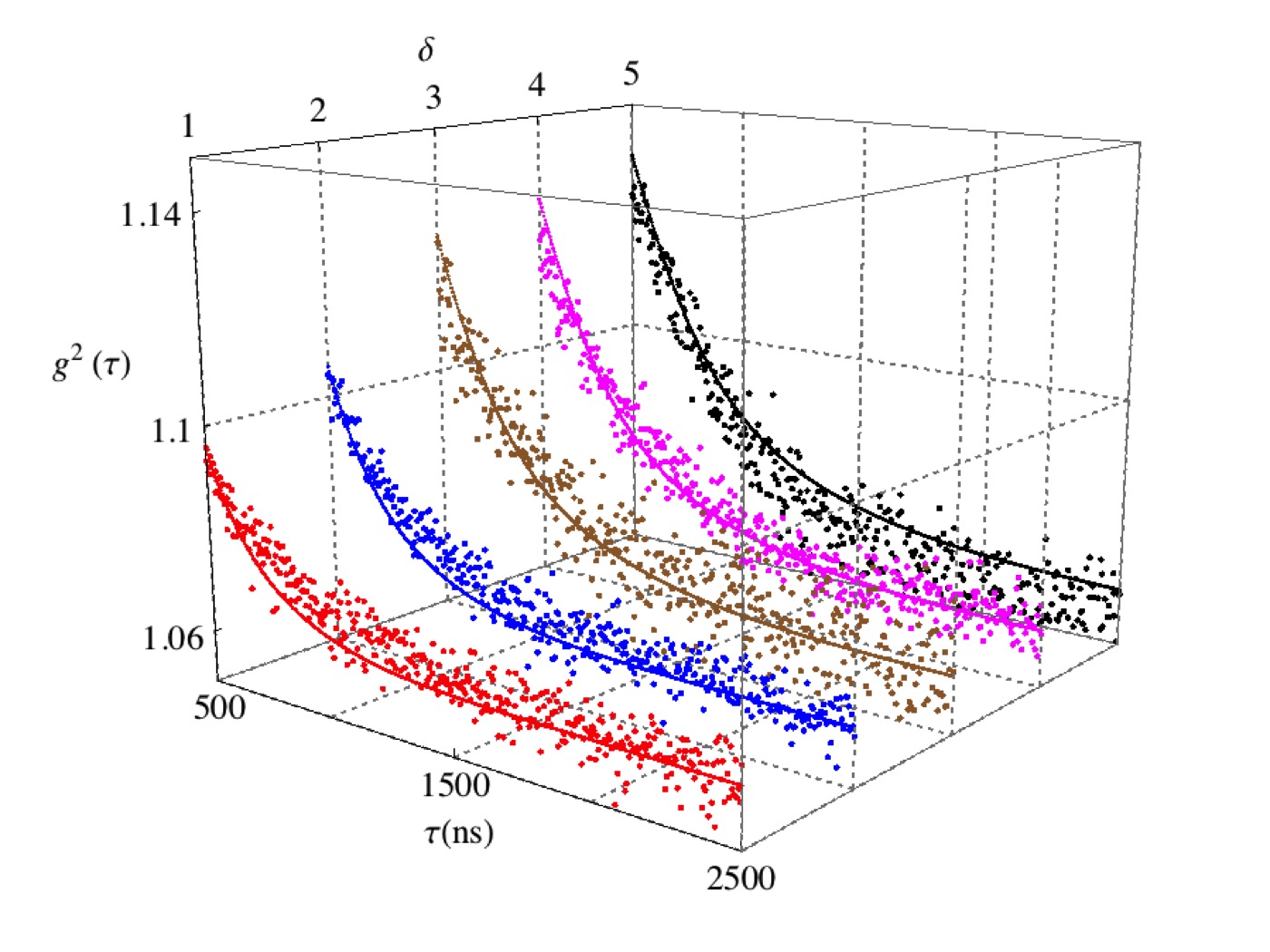
Figure 3: $g^{(2)}(\tau)\,\,$vs $\tau$ for different detunings, $\delta$ (1 = -14.5MHz, 2 = -16.1MHz, 3 = -18MHz, 4 = -19.4MHz, 5 = -22MHz) of the cooling beam from the cooling transition. The values obtained from TDII measurements are shown as dots. The solid curves represent the values of $g^{(2)}(\tau)\,\,$obtained from Eqs.7 and 9, with temperatures $100\mu$K, $80\mu$K, $60\mu$K, $50\mu$K, $43\mu$K, for the 5 values of detunings, (1 = -14.5MHz, 2 = -16.1MHz, 3 = -18MHz, 4 = -19.4MHz, 5 = -22MHz) respectively. The data for all sets are fit with the same choice of parameters, to obtain the temperature.

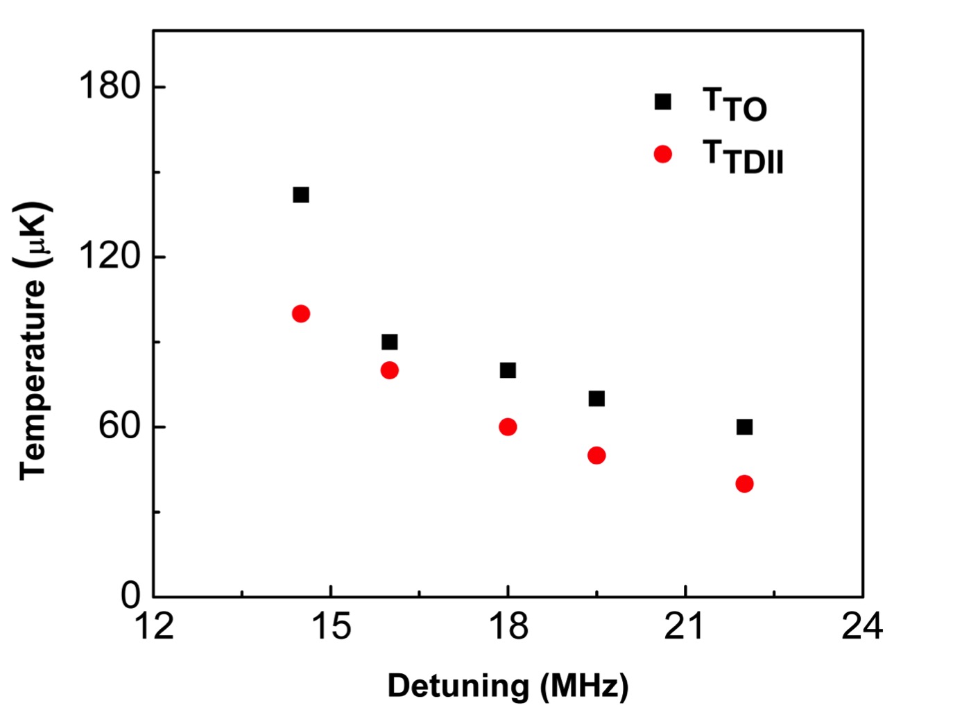
Figure 4: Comparison of the temperature of the cold atoms, obtained from two methods - TDII (circles) and trap oscillation (squares) - as function of the (red) detuning of the cooling beam.

We now turn our attention to the remaining observation - the increase in $g^{(2)}(0)\,\,$with detuning. We attribute this to the timing resolution in our experiment. The larger the detuning, the colder the collection of atoms, and hence the slower the decay in coherence. Thus the timing resolution of 5ns appears adequate for large detunings. For hotter atoms obtained at lower detunings, the averaging effect of the time bin becomes discernible, as it is now a larger fraction of the coherence time.

As pointed out earlier, though light form a thermal collection of atoms is expected to exhibit a second-order intensity correlation of 2, this value could not be experimentally obtained till very recently; in fact, the present work and that of Nakayama and coworkers Nakayama are the only two reports of this. Further, there has been skepticism on being able to obtain a good measure of bunching, and of being able to see coherent effects in TDII measurements from a collection of large number of atoms Gomer . Several factors have contributed to the difficulty in observing the theoretically predicted behaviour. All researchers have stressed on the need for good timing resolution, which in the present case is 5ns. However, small time bins necessitate longer acquistion times to obtain good statistics, making the experiment long and tedious. Light has to be collected over a single spatial coherence region, contributing to further reduction in photon counts. These factors require the experimental setup to be extremely stable, and the conditions repeatable over nearly ten hours. Another factor known to degrade the observation of bunching is the presence of a magnetic field Bali , because of which all measurements hitherto had atoms cooled in a MOT and then transferred to a molasses, either by switching off the magnetic field (Bali ; Aspect ), or by transporting the atoms to another vacuum chamber Nakayama . Our experiment, however, has been carried out in-situ, with atoms in a MOT, with all cooling and repumper beams and the quadrupolar magnetic field present. Good mechanical isolation of the setup and temperature stability of the environment ensured that the lasers remained locked for the entire duration of the experiment. Constant monitoring of the MOT fluorescence allowed for corrective measures, which, however, were not required. The diffraction-limited collection lens placed within the MOT chamber, in close proximity to the cold atoms, and the subsequent spatial filtering enabled us to collect light from a small region of the MOT, over which the magnetic field was uniform within 2mG, eliminating broadening due to Zeeman shift. Likewise, the low temperature, and the thus the sub-natural Doppler width ensured that the Rabi frequency is the same for all atoms. Further, the small size of the cold cloud ($400\mu$m across), the low number of atoms ensured that reabsorption of the emitted light was negligible. This allowed us to detect coherent effects like Rabi oscillations. In an earlier study, single atom dynamics was probed by photon-photon correlation in an optical dipole trapGomer , where one, two, or three atoms were held trapped. In the present experiment, the number of atoms contributing to the collected light is three orders of magnitude higher. Further, atoms move in and out of the region from which light is collected, due to the thermal motion, and the superimposed trap oscillation in the quadrupolar magnetic field. The transit time of an atom (in the absence of a collision that expels it from this region), is estimated to be $\sim 10\mu$s. The power of TDII is brought out in the present study, where, despite the sample being a thermal collection of several thousand atoms, coherent dynamics are revealed.
In conclusion, we have perfomed Time-Delayed Intensity Interferometry with light emitted by an ultracold atomic ensemble in a steady state MOT. The collection of cold atoms is a source of bunched light, where bunching is introduced by spontaneous emission. Well defined, but decaying Rabi oscillatons were seen at small time delays ($<150$ns) that give way to an exponential decay at larger time delays. It is thus seen that TDII measurements enable the study of coherent and incoherent dynamics of the system, providing a relative measure of the various dynamical processes occuring at different time scales, even from a thermal ensemble of a large number of independent atoms.
Acknowledgements : We thank Ms. M.S. Meena for her efficient help in electronics related to the setting up of the MOT. We gratefully acknowledge Prof. G. S. Agarwal for several detailed discussions and for the theoretical treatment presented here.

References

- (1) R. Hanbury Brown and R. Q. Twiss, Nature 177, 27 (1956).
- (2) Gordon Baym, Acta Physica Polonica, 29, 1839 (1998).
- (3) R. Lednicky, Brazilian Journal of Physics, 37, 939, 2007
- (4) C. Foellmi, Astr. Astrophy., 507, 1719-1727 (2009).
- (5) M. Assmann, F. Veit, J. Tempel,T. Berstermann, H. Stolz, M. van der Poel, J. M. Hvam, and M. Bayer, Opt. Exp., 18, 20229 (2010).
- (6) http, www.lsinstruments.ch,technology,dynamic,light, scattering,dls
- (7) D.T. Philips, Herbert Kleiman and Sumner P. Davis, Phys. Rev. 153, 113 (1966).
- (8) W. Martienssen and E. Spiller, Am J Phys (1964).
- (9) A. Martin, O. Alibert, J.C. Flesch, J. Samuel, Supurna Sinha, S. Tanzilli, and A. Kastberg, EPL 1, 10003 (2012).
- (10) Nandan Satapathy, Deepak Pandey, Poonam Mehta, Supurna Sinha, Joseph Samuel, and Hema Ramachandran, EPL 97, 50011 (2012).
- (11) Nandan Satapathy, Deepak Pandey, Sourish Banerjee, and Hema Ramachandran, J. Opt. Soc. Am. A, 30, 910 (2013).
- (12) Deepak Pandey, Nandan Satapathy, Buti Suryabrahmam, J. Solomon Ivan and Hema Ramachandran, Eur. Phys. J. Plus 129, 115 (2014).
- (13) C. Jurczak, B. Desruelle, K. Sengstock, J.-Y. Courtois, C. I. Westbrook, and A. Aspect, Phys. Rev. Lett., 77, 1727 (1996)
- (14) S. Bali, D. Hoffmann, J. Siman, and T. Walker, Phys. Rev. A 53, 3469 (1996).
- (15) K. Nakayama, Y. Yoshikawa, H. Matsumoto, Y. Torii1, and T. Kug, Opt. Exp. 18, 6604 (2010).
- (16) Manuscript under preparation.
- (17) P. Kohns, P. Buch, W. Suptitz, C. Csambal and W. Ertmer, Europhys. Lett., 22, 517 (1993).
- (18) Chapter 13, Quantum Optics by Girish S. Agarwal, Cambridge University Press, 2012.
- (19) V. Gomer, F. Strauch, B. Ueberholz, S. Knappe, and D. Meschede, Phys. Rev. A 58, R1657 (1998).
- (20) C. I. Westbrook, R. N. Watts, C. E. Tanner, S. L. Rolston, W. D. Phillips, and P. D. Lett, Phys. Rev. Lett., 65, 33 (1990).