Inter-community resonances in multifrequency ensembles of coupled oscillators

Abstract

We generalize the Kuramoto model of globally coupled oscillators to multifrequency communities. A situation when mean frequencies of two subpopulations are close to resonance 2:1 is considered in detail. We derive uniformly rotating solutions describing synchronization inside communities and between them. Remarkably, cross-coupling between the frequency scales can promote synchrony even when ensembles are separately asynchronous. We also show that the transition to synchrony due to the cross-coupling is accompanied by a huge multiplicity of distinct synchronous solutions what is directly related to a multi-branch entrainment. On the other hand, for synchronous populations, the cross-frequency coupling can destroy a phase-locking and lead to chaos of mean fields.

I Introduction

Models in the form of coupled oscillators are ubiquitous in various scientific fields, ranging from physics and chemistry (Wiesenfeld and Swift, 1995; *Wiesenfeld-Colet-Strogatz-96; *Wiesenfeld-Colet-Strogatz-98; *Kiss-Zhai-Hudson-02a; *Grollier-Cros-Fert-06; *georges:232504) to biology (Golomb et al., 2001; *Breakspear-Heitmann-Daffertshofer-10; *Gonze-05; *Bordyugov-13), as well as in some interdisciplinary applications (Eckhardt et al., 2007; *Neda_etal-00). In many cases dynamics of oscillatory ensemble can be successfully studied in the phase approximation  (Kuramoto, 1984; Pikovsky et al., 2001). When the coupling between the oscillators is relatively weak, one can neglect changes in the amplitude dynamics of natural limit cycles of the oscillators, and describe the system in terms of the phases only. This technique is known as phase reduction, and it represents, basically, one of the few rigorous mathematical approaches to study complex non-equilibrium nonlinear oscillatory dynamics.

The simplest setup here represents a globally coupled ensemble with weak interaction and relatively close natural frequencies. The phase reduction here leads to the system of globally coupled phase equations where interaction between the oscillators is described by $2\pi$ - periodic function of phase differences  (Kuramoto, 1984, 1975; Izhikevich, 2007; *Izhikevich-00; Daido, 1993a; *Daido-93a; *Daido-96; *Daido-95). The classical and well-studied Kuramoto-Sakaguchi model appears when one consider only the first Fourier mode in the interaction function what leads to simple sinusoidal coupling. There is almost 40 years of intensive studies dedicated to explanation of bifurcations and dynamics in this model (Acebrón et al., 2005). A surprising recent result discovered a possibility of low-dimensional description of the classical Kuramoto model in terms of macroscopic order parameters (Watanabe and Strogatz, 1994; Ott and Antonsen, 2008; *Ott-Antonsen-09; Marvel et al., 2009; *Pikovsky-Rosenblum-08; *Pikovsky-Rosenblum-11). However, this reduction to low-dimensional systems does not imply simplicity of dynamical behavior. In opposite, the authors (Omel’chenko and Wolfrum, 2012; *Omelchenko-Wolfrum-13) report on quite complicated phase transitions and bifurcations in the Kuramoto-Sakaguchi models.

The cases of multi-harmonic coupling functions (Daido, 1995, 1996b, 1996a; *Crawford-95; *Crawford-Davies-99; *Chiba-Nishikawa-11; *Hansel-93; *Ashwin_etal-07) appear to be more complicated and usually responsible for new dynamical effects in comparison to classical setup with purely sinusoidal function. In large ensembles the multi-harmonic case leads to appearance of so-called multi-branch entrainment modes with a huge multiplicity of possible synchronous solutions (Daido, 1995, 1996b; Komarov and Pikovsky, 2013a; *Komarov-Pikovsky-14). The latter also leads to non-trivial noise-induced effects (Vlasov et al., 2015).

One of the directions in this growing theoretical field is dedicated to multi-frequency oscillator communities. As it was mentioned before, the Kuramoto-type models were obtained under assumptions of weak coupling limit and closeness of natural oscillator frequencies. However, when the distribution of the frequencies is huge in comparison to the interaction strength, the phase reduction leads to another types of phase models  (Lück and Pikovsky, 2011; Komarov and Pikovsky, 2013b, 2011). A natural setup here implies existence of a certain number of oscillator subpopulations (communities), such that the frequencies inside each population are close, but differ significantly across the distinct communities. This situation is inspired by theoretical and experimental results from neuroscience (Buzsáki, 2006; *Rosjat-Popovych-Daun-14), indicating that distinct interacting brain areas exhibit different natural oscillatory rhythms.

In this paper we consider a particular problem when distinct oscillatory communities have natural frequencies close to a high-order resonance. First, we derive general phase equations for globally interacting ensembles and distinguish different types of resonant coupling which may appear in the system. Next, we concentrate on the simplest case of two interacting population whose mean frequencies are close to an 2:1 resonance. The aim of the paper is to demonstrate on this simplest example, what one can expect from the effects high-order resonances. To describe the dynamics, we adopt the self-consistent approach developed in (Komarov and Pikovsky, 2014) for calculation of stationary order parameters for multi-harmonic coupling functions. Our analysis will show that the model exhibits reach dynamical behavior including multi-branch entrainment (multiplicity) and chaotic collective oscillations.

II Phase equations for resonantly coupled populations

In this section we will present a general scheme of coupling in resonant, multifrequency populations of oscillators. We will assume that each oscillator is described solely by its phase $\phi$, which satisfies the following equation

$$\dot{\phi}=\omega+S(\phi)F$$

where $\omega$ is oscillator’s natural frequency, $S(\phi)$ is its phase response curve, and $F$ is the force acting from other oscillators. In order to simplify notations, we from the beginning will consider a thermodynamic limit, where the number of units in all populations and subpopulations tends to infinity (although at the end we will also write the governing equations for a finite size case). We assume that the ensemble is divided into $M$ distinct subpopulations (we will use index $n$ for referring to them), around $M$ distinct mean frequencies $\overline{\omega}_{n}$. Additionally, there can be a small deviation from the mean frequency $\Delta$ (typically described by a unimodal distribution around zero). We now introduce slow phases, by writing explicitly fast rotating terms $\sim\overline{\omega}_{n}t$. In fact, we can also chose frequencies of fast rotations $\Omega_{n}$ to be close, but not exactly equal, to $\overline{\omega}_{n}$. We will use this freedom to be able to make perfect averaging below. Our slow phases $\varphi_{n}(\Delta)=\phi_{n}-\Omega_{n}t$ satisfy equations

$$\dot{\varphi}_{n}(\Delta)=\Delta+S_{n}(\Omega_{n}t+\varphi_{n})F_{n}$$ (1)

where now individual mismatches $\Delta$ for the group $n$ are distributed generally asymmetrically, with some small shift $\sim\overline{\omega}_{n}-\Omega_{n}$.

Next, we assume that coupling between the groups and inside each group is due to mean fields only. These mean fields for each subpopulation are represented by generalized order parameters

$$Z_{k}^{(n)}=\langle e^{ik(\Omega_{n}t+\varphi_{n})}\rangle=\overline{Z}_{k}^{(n)}e^{ik\Omega_{n}t}$$

where averaging is over the distribution of the slow phases following from (1) and over the distribution of $\Delta$. The introduced order parameters $\overline{Z}$ are slow functions of time as they are defined via the slow phases:

$$\overline{Z}k^{(n)}=\langle e^{ik\varphi_{n}}\rangle$$ (2)

In general, the force acting on the oscillators of the group $n$ is from all other groups, and is a nonlinear function of order parameters, which one can expand in powers of them. We, however, in this paper will restrict ourselves to the linear coupling only, i.e. we will assume that $F_{n}$ is a linear function of order parameters:

$$F_{n}(Z_{k}^{(1)},Z_{k}^{(2)},\ldots)=\sum_{k,m}h_{n,k}^{(m)}Z_{k}^{(m)}=\sum_{k,m}h_{n,k}^{(m)}\overline{Z}_{k}^{(m)}e^{ik\Omega_{m}t}$$ (3)

Representing the phase response function $S_{n}$ as a Fourier series

$$S_{n}(\phi)=\sum_{p}s_{np}e^{ip\phi}$$

and substituting this in Eq. (1), we obtain

$$\dot{\varphi}_{n}(\Delta) =\Delta+\sum_{p}s_{np}e^{ip\varphi}e^{ip\Omega_{n}t}\left[\sum_{k,m}h_{n,k}^{(m)}\overline{Z}_{k}^{(m)}e^{ik\Omega_{m}t}\right]=$$ (4)

$$=\Delta+\sum_{p,k,m}s_{np}h_{n,k}^{(m)}\overline{Z}_{k}^{(m)}e^{ip\varphi}e^{i(p\Omega_{n}+ik\Omega_{m})t}$$

Now one has to perform averaging of Eq. (4), to reveal evolution of the slow phase. The fast terms on the r.h.s. are those containing explicit time dependence with one of the frequencies $\Omega_{n}$ or with a combination of them. Such a combination can be small, this is exactly the case of a resonance that is of special interest for us. Here, we use the freedom in the choice of particular values of $\Omega_{n}$, to make the resonance exact. This means that some combination of frequencies $\Omega_{n}$ vanishes exactly. Performing averaging means just keeping these terms on the r.h.s. of Eq. (4), and neglecting all other containing explicit time dependence.

Expansion (4) can be treated in many setups of particular resonant conditions, we describe here some evident cases:

• One population of oscillators. In this case only one frequency $\Omega$ exists. Here the only terms surviving the averaging are those with $p+k=0$, this leads to the Daido model Daido (1993a); *Daido-93a; *Daido-96; *Daido-95.

• Two subpopulations. Here the main interest is in the resonance of two frequencies $\Omega_{1},\Omega_{2}$. The simplest case is just the second-harmonic resonance: $\Omega_{2}=2\Omega_{1}$. In this case only those cross-population coupling terms with $p+2k=0$ survive. Similarly, for high-order resonances like $a\Omega_{2}=b\Omega_{1}$ (with integer $a,b$) the terms with $ap+bk=0$ contribute.

• More than two subpopulations. One can see from (4), that in the case of linear coupling, there is no direct interaction involving more that two subpopulations. So the resulting coupling is a combination of terms stemming from pairwise resonances.

We restrict ourself in this paper to the simplest case of two resonant subpopulations with $\Omega_{2}=2\Omega_{1}$. As described above, after averaging only terms where combinations $\sim(\Omega_{1,2}-\Omega_{1,2})$ and $\sim(\Omega_{2}-2\Omega_{1})$ appear, survive, for the interaction within one and between subpopulations, respectively:

$$\dot{\varphi}_{1}(\Delta) =\Delta+\sum_{k}s_{1,-k}h_{1,k}^{(1)}\overline{Z}_{k}^{(1)}e^{-ik\varphi_{1}}+\sum_{k}s_{1,-2k}h_{1,k}^{(2)}\overline{Z}_{k}^{(2)}e^{-i2k\varphi_{1}}$$ (5)

$$\dot{\varphi}_{2}(\Delta) =\Delta+\sum_{k}s_{2,-k}h_{2,k}^{(2)}\overline{Z}_{k}^{(2)}e^{-ik\varphi_{2}}+\sum_{k}s_{2,-k}h_{2,2k}^{(1)}\overline{Z}_{2k}^{(1)}e^{-ik\varphi_{2}}$$

We now insert here the definition of the slow order parameters (2) and obtain

$$\dot{\varphi}_{1}(\Delta) =\Delta+\langle\sum_{k}s_{1,-k}h_{1,k}^{(1)}e^{ik(\tilde{\varphi}_{1}-\varphi_{1})}\rangle+\langle\sum_{k}s_{1,-2k}h_{1,k}^{(2)}e^{ik(\tilde{\varphi}_{2}-2\varphi_{1})}\rangle$$ (6)

$$\dot{\varphi}_{2}(\Delta) =\Delta+\langle\sum_{k}s_{2,-k}h_{2,k}^{(2)}e^{ik(\tilde{\varphi}_{2}-\varphi_{2})}\rangle+\langle\sum_{k}s_{2,-k}h_{2,2k}^{(1)}e^{ik(2\tilde{\varphi}_{1}-\varphi_{2})}\rangle$$

where averaging is over variables with tilde. Now we can define effective coupling functions inside subpopulations $f_{11},f_{22}$ and coupling functions across subpopulation $f_{12},f_{21}$ as

$$f_{11}(\phi)=\sum_{k}s_{1,-k}h_{1,k}^{(1)}e^{ik\phi}\qquad f_{22}(\phi)=\sum_{k}s_{2,-k}h_{2,k}^{(2)}e^{ik\phi}$$ (7)

$$f_{12}(\phi)=\sum_{k}s_{1,-2k}h_{1,k}^{(2)}e^{ik\phi}\qquad f_{21}(\phi)=\sum_{k}s_{2,-k}h_{2,2k}^{(1)}e^{ik\phi}$$

Now we can formulate equations for finite populations, replacing $\langle\rangle$ by corresponding sums. We assume that subpopulations 1 and 2 have $N_{1}$ and $N_{2}$ units, respectively. Furthermore, one can now also transform back to the original fast phases, because in the averaged formulation the absolute values of the frequencies do not play any rôle. Denoting the phases in the subpopulation at a smaller frequency (we will also call it the first subpopulation below) as $\phi_{p}$, and the phases in the subpopulation at a larger frequency (referred hereafter as the second subpopulation) as $\psi_{p}$, we get

$$\dot{\phi}_{q} =\omega_{q}+\frac{1}{N_{1}}\sum_{k=1}^{N_{1}}f_{11}(\phi_{k}-\phi_{q})+\frac{1}{N_{2}}\sum_{p=1}^{N_{2}}f_{12}(\psi_{p}-2\phi_{q})$$ (8)

$$\dot{\psi}_{q} =\nu_{q}+\frac{1}{N_{2}}\sum_{k=1}^{N_{2}}f_{22}(\psi_{k}-\psi_{q})+\frac{1}{N_{1}}\sum_{p=1}^{N_{1}}f_{21}(2\phi_{p}-\psi_{q})$$

where we also have split notations for frequencies in two subpopulations. This system is a generalization of the Daido model Daido (1993a); *Daido-93a; *Daido-96; *Daido-95 to two resonantly coupled ensembles. Below we will consider the case where coupling functions $f$ contain the first harmonics only; this will correspond to the Kuramoto-Sakaguchi-type coupling. In this case each coupling function is determined by two parameters, the amplitude and the phase shift. One of the phase shifts in the cross-coupling can be set to zero by shifting all the phases in one subpopulation with respect to another one. Thus, our coupling functions will be:

$$f_{11}(x)=\varepsilon_{1}\sin(x-\alpha_{1}),\quad f_{22}(x)=\varepsilon_{2}\sin(x-\alpha_{2}),\quad f_{12}(x)=\gamma_{1}\sin(x-\beta),\quad f_{22}(x)=\gamma_{2}\sin x$$

Next, we fix the distributions of the frequencies. As after the averaging the system is invariant under transformation $\phi\to\phi+2At$, $\psi\to\psi+At$ for arbitrary $A$, we can set the average value of the natural frequencies in the first subpopulation $\phi$ to zero, the average frequency $\delta$ in the second subpopulation is the relevant parameter responsible for the mismatch. We will assume the frequencies to be distributed according to Lorentzian distributions, with equal widths. Because we still have a freedom of changing the time scale, we will assume that this width is one:

$$g_{1}(\omega)=\frac{1}{\pi(\omega^{2}+1)}\qquad g_{2}(\nu)=\frac{1}{\pi((\nu-\delta)^{2}+1}$$ (9)

The resulting microscopic system of oscillators to be considered below reads

$$\dot{\phi}_{n}=\omega_{n}+\frac{\varepsilon_{1}}{N_{1}}\sum_{k=1}^{N_{1}}\sin(\phi_{k}-\phi_{n}-\alpha_{1})+\frac{\gamma_{1}}{N_{2}}\sum_{k=1}^{N_{2}}\sin(\psi_{k}-2\phi_{n}-\beta)$$ (10)

$$\dot{\psi}_{m}=\nu_{m}+\frac{\varepsilon_{2}}{N_{2}}\sum_{k=1}^{N_{2}}\sin(\psi_{k}-\psi_{m}-\alpha_{2})+\frac{\gamma_{2}}{N_{1}}\sum_{k=1}^{N_{1}}\sin(2\phi_{k}-\psi_{m})$$

with frequencies defined according to the distributions (9).

We now also write down the basic equations in the thermodynamic limit. Here three complex order parameters $\mathbf{X}_{1},\mathbf{X}_{2},\mathbf{Y}$ appear defined as

$$\mathbf{X}_{k} =X_{k}e^{i\Theta_{k}}=\langle e^{ik\phi}\rangle=\iint d\phi d\omega\;g_{1}(\omega)\rho(\phi|\omega)e^{ik\phi},\qquad k=1,2\;,$$ (11)

$$\mathbf{Y} =Ye^{i\Theta_{y}}=\langle e^{i\psi}\rangle=\iint d\psi d\nu\;g_{2}(\nu)\rho(\psi|\nu)e^{i\psi}$$

while equations for the phases are

$$\dot{\phi} =\omega+\varepsilon_{1}X_{1}\sin(\Theta_{1}-\phi-\alpha_{1})+\gamma_{1}Y\sin(\Theta_{y}-2\phi_{1}-\beta)$$ (12)

$$\dot{\psi} =\nu+\varepsilon_{2}Y\sin(\Theta_{y}-\psi-\alpha_{2})+\gamma_{2}X_{2}\sin(\Theta_{2}-\psi)$$

The formulated system of equation will be subject of our analysis below, where we will concentrate on main dynamical effects caused by resonant cross-coupling. In numerical simulations we will use microscopic equations (10), while in the theoretical construction the thermodynamic limit formulation (11,12) will be used.

III Self-consistent solutions in the thermodynamic limit

Here we will present the self-consistent scheme allowing us to find stationary (or, more generally, uniformly rotating) synchronous solutions of the system (11,12).

III.1 Ott-Antonsen ansatz for the second subpopulation

The problem partially simplifies by the observation, that for the subpopulation $\psi$ at the double frequency the Ott-Antonsen ansatz Ott and Antonsen (2008); *Ott-Antonsen-09 can be applied. Indeed, the second of eqs. (12) can be rewritten as

$$\dot{\psi}=\nu+\text{Im}(\mathbf{H}(t)e^{-i\psi}),\quad\mathbf{H}=\varepsilon_{2}e^{-i\alpha_{2}}\mathbf{Y}+\gamma_{2}\mathbf{X}_{2}$$ (13)

According to the Ott-Antonsen theory, equation for the order parameter $\mathbf{Y}$ obeys (under some additional assumptions which we assume to be satisfied here), in the case of a Lorentzian distribution (9), an ODE

$$\dot{\mathbf{Y}}=\mathbf{Y}(i\delta-1)-\frac{1}{2}(\mathbf{H}^{*}\mathbf{Y}^{2}-\mathbf{H})=\mathbf{Y}(i\delta-1)-\frac{\varepsilon_{2}\mathbf{Y}}{2}(e^{-i\alpha_{2}}|\mathbf{Y}|^{2}-e^{i\alpha_{2}})-\frac{\gamma_{2}}{2}(\mathbf{X}_{2}^{*}\mathbf{Y}^{2}-\mathbf{X}_{2})$$ (14)

III.2 Uniformly rotating ansatz

We now construct solution for the ensemble of oscillators $\varphi$. Here we cannot use the Ott-Antonsen ansatz, because the latter is only applicable for the driving terms possessing one harmonics of the phase, like in (13). The equations for $\varphi$ possesses both the first and the second harmonics. In order to find stationary values of the mean fields, we will adapt the self-consistent scheme developed in Refs. (Komarov and Pikovsky, 2013a; *Komarov-Pikovsky-14) for the deterministic bi-harmonic Kuramoto model (for the noisy case a similar method can be used, see (Vlasov et al., 2015; Komarov et al., 2014)).

In this self-consistent approach one finds uniformly rotating distributions, i.e. distributions that are stationary in a rotating reference frame. Let us denote the frequency of this frame $\Omega$, it will be determined self-consistently as a result of the calculations. According to this, we introduce constant phases of the order parameters

$$\Theta_{1}=\Omega t,\quad\theta_{2}=\Theta_{2}-2\Omega t,\quad\theta_{y}=\Theta_{y}-2\Omega t$$ (15)

(here the phase shift of the first order parameter $\mathbf{X}_{1}$ is set to zero, this can be always done by the time shift). Also, we introduce a new phase variable

$$\varphi=\phi-\Omega t+\alpha_{1}$$

distribution of which is expected to be stationary. This variable obeys

$$\dot{\varphi}=\omega-\Omega+\varepsilon_{1}X_{1}\sin(-\varphi)+\gamma_{1}Y\sin(\theta_{y}+2\alpha_{1}-\beta-2\varphi)$$ (16)

III.3 Stationary solution in a parametric form

To proceed with self-consistent solution, it is convenient to introduce four auxiliary parameters $\{R,\ u,\ v,\ z\}=\mathbf{P}$ in the following way:

$$\varepsilon_{1}X_{1}=R\sin{u},\ \gamma_{1}Y=R\cos{u},\ \Omega=zR,\ v=\theta_{y}+2\alpha_{1}-\beta$$ (17)

Now (16) takes the following form:

$$\dot{\varphi}=R\left(x-z-\sin{u}\sin{\varphi}-\cos{u}\sin(2\varphi-v)\right)=R\left(x-z-h(u,v,\varphi)\right)$$ (18)

We denoted $x=\omega/R$ and $h(u,v,\varphi)=\sin u\sin\varphi+\cos u\sin(2\varphi-v)$. At some constant values of parameters $\mathbf{P}$ in (18), at each value of $x$ one can find stationary distribution function $\rho(\varphi|x,\mathbf{P})$, and then calculate the corresponding complex order parameters:

$$X_{1} =e^{-i\alpha_{1}}R\iint\rho(\varphi|x,\mathbf{P})e^{i\varphi}g(Rx)dxd\varphi=e^{i(\theta_{1}-\alpha_{1})}RF_{1}(\mathbf{P})e^{iQ_{1}(\mathbf{P})}$$ (19)

$$X_{2}e^{i\theta_{2}} =e^{-i2\alpha_{1}}R\iint\rho(\varphi|x,\mathbf{P})e^{i2\varphi}g(Rx)dxd\varphi=e^{-i2\alpha_{1}}RF_{2}(\mathbf{P})e^{iQ_{2}(\mathbf{P})}$$

$$F_{m}(\mathbf{P})e^{iQ_{m}(\mathbf{P})} \equiv\iint dxd\varphi\rho(\varphi|x,\mathbf{P})e^{im\varphi}g(Rx)\;,\qquad m=1,2\;.$$

Our next goal is to calculate the integrals $F_{m}(\mathbf{P})$, for this we need to find, using the dynamical equation (18), the stationary distribution function $\rho(\varphi|x,\mathbf{P})$. Let $H_{min}$ and $H_{max}$ denote the global minimum and the global maximum of function $h(u,v,\varphi)$, correspondingly (Fig.1(b)). All the oscillators can be separated into locked ones (for $H_{max}\geq|x-z|\geq H_{min}$) or rotating, unlocked ones ($x-z>H_{max}$ or $x-z<H_{min}$). The distribution function of rotating oscillators (index $r$) is inversely proportional to their phase velocity:

$$\rho_{r}(\varphi|x,\mathbf{P})=\frac{C(x)}{|x-z-h(\varphi,u,v)|}\;,$$ (20)

where $C(x)$ is the normalization constant:

$$C(x)=\frac{1}{\int_{0}^{2\pi}\frac{d\varphi}{|x-z-y|}}.$$

The stationary phases of locked oscillators (index $l$) can be found from the following relation:

$$x-z=h(u,v,\varphi)\;.$$ (21)

(a)

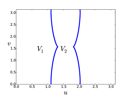
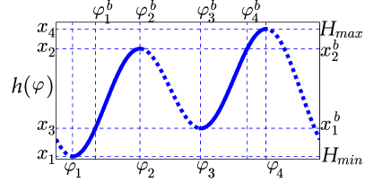
(b) (c)

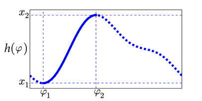
Figure 1: (a) Regions $V_{1}$ and $V_{2}$ in the plane of parameters $(u,v)$: Domain $V_{1}$ corresponds to a double-well form of function $h(u,v,\varphi)$ (Fig. 1(b,d)), while in $V_{2}$ $h(u,v,\varphi)$ has a single-well form like sown in Fig. 1(c). (b) Example of function $h(u,v,\varphi)$ with 4 extrema is presented. There are two stable branches (solid curves) for stationary phases of locked oscillators. The left branch $\varphi=\Psi_{1}(x,\mathbf{P})$ is larger than the right one $\varphi=\Psi_{2}(x,\mathbf{P})$. $(\varphi_{1,2},x_{1,2})$ denote coordinates of the extrema corresponding to the branch $\Psi_{1}$, while $(\varphi_{3,4},x_{3,4})$ denotes extrema at $\Psi_{2}$. In the domain $h(\varphi)\in[x^{b}_{1},x^{b}_{2}]$ there is a bistability on the microscopic level: in this domain the oscillators can be locked either on the branch $\Psi_{1}$ in the range $\varphi\in[\varphi^{b}_{1},\varphi^{b}_{2}]$ or on the branch $\Psi_{2}$ in the range $\varphi\in[\varphi^{b}_{3},\varphi^{b}_{4}]$. (c) Example of function $h(u,v,\varphi)$ with only two extrema and one stable branch $\varphi=\Psi_{1}(x,\mathbf{P})$ (solid curve).

When finding $\varphi$ as a function of $x$ for non-rotating (locked, index $l$) phases, we have to satisfy an additional stability condition $\frac{\partial h(u,v,\varphi)}{\partial\varphi}>0$ that follows from the dynamical equation (18). In the $(u,v)$ plane there are two regions $V_{1}$ and $V_{2}$ (Fig. 1(a)) with qualitatively different properties of the system (18) and different types of distribution function $\rho_{l}(\varphi|x,\mathbf{P})$, correspondingly:

$\{u,v\}\in V_{1}$

In this case function $h(u,v,\varphi)$ has a double-well form like shown in Fig.1(b). According to (18), oscillators can be located on two possible stable branches highlighted by solid curves in Fig.1(b): the first branch is $\varphi=\Psi_{1}(x,\mathbf{P})$ in the range $\varphi\in[\varphi_{1},\varphi_{2}]$ and another branch is $\varphi=\Psi_{2}(x,\mathbf{P})$ for $\varphi\in[\varphi_{3},\varphi_{4}]$. Here and below we assume $\Psi_{1}(x,\mathbf{P})$ to be the biggest stable branch. In the range $(x-z)\in(x^{b}_{1},x^{b}_{2})$ (Fig. 1(b)) there is an area of bistability on the microscopic level: the oscillators with the same natural frequency $x$ can be locked at two different phases $\Psi_{1}(x,\mathbf{P})$ and $\Psi_{2}(x,\mathbf{P})$. Therefore, the distribution function has the following form:

$$\rho_{l}(\varphi|x,\mathbf{P})=\left\{\begin{array}[]{l}(1-S(x))\delta(\psi-\Psi_{1}(x,\mathbf{P}))+S(x)\delta(\varphi-\Psi_{2}(x,\mathbf{P}))\\ \text{for $(x-z)\in[x^{b}_{1},x^{b}_{2}]$}\;,\\ \delta(\varphi-\Psi_{1}(x,\mathbf{P}))\ \ \ \text{for $(x-z)\in[x_{1},x_{2}]\setminus[x_{1}^{b},x_{2}^{b}]$}\;,\\ \delta(\varphi-\Psi_{2}(x,\mathbf{P}))\ \ \ \text{for $(x-z)\in[x_{3},x_{4}]\setminus[x_{1}^{b},x_{2}^{b}]$}\;.\\ \end{array}\right.$$ (22)

Here $0\leq S(x)\leq 1$ is an indicator function describing the redistribution over the stable brunches; this function is arbitrary.

$\{u,v\}\in V_{2}$

In the second case, function $h(u,v,\psi)$ has only two extrema (Fig. 1(c)) and there is only one stable branch $\varphi=\Psi_{1}(x,\mathbf{P})$. The distribution function is:

$$\rho_{l}(\varphi|x,\mathbf{P})=\delta(\varphi-\Psi_{1}(x,\mathbf{P}))\ \text{for $x\in(z+x_{1},z+x_{2})$}\;.$$ (23)

Taking into account the obtained expressions for the distribution function (20,22,23), the integrals in (19) can be rewritten as a sum of five terms:

$$F_{m}(\mathbf{P})e^{iQ_{m}(\mathbf{P})}=\int_{\varphi_{1}}^{\varphi_{2}}d\varphi e^{im\varphi}g\left(R(z+h)\right)\frac{\partial h}{\partial\varphi}-$$ (24)

$$\int_{\varphi^{b}_{1}}^{\varphi^{b}_{2}}d\varphi e^{im\varphi}S(z+h)g\left(R(z+h)\right)\frac{\partial h}{\partial\varphi}+\int_{\varphi_{3}}^{\varphi_{4}}d\varphi e^{im\varphi}g\left(R(z+h)\right)\frac{\partial h}{\partial\varphi}-$$

$$\int_{\varphi^{b}_{3}}^{\varphi^{b}_{4}}d\varphi e^{im\varphi}\left(1-S(z+h)\right)g\left(R(z+h)\right)\frac{\partial h}{\partial\varphi}+\int_{\mathcal{X}}\int_{0}^{2\pi}dxd\varphi\frac{g(Rx)C(x)e^{im\varphi}}{|x-z-h|}\;.$$

Here the first and the second terms stand for integration over the first branch $\Psi_{1}$ in the range $[\varphi_{1},\varphi_{2}]$. The second term accounts for certain redistribution $S(x)$ of oscillators between the branches in the range $[\varphi_{1}^{b},\varphi_{2}^{b}]$ (Fig. 1(b)). Similarly, the third and the fourth terms correspond to integration over the possible stable branch $\Psi_{2}$ in the range $[\varphi_{3},\varphi_{4}]$. In the same way, the fourth term accounts for redistribution of oscillators between branches in the range $[\varphi_{3}^{b},\varphi_{4}^{b}]$ (Fig. 1(b)). In the last term the interval $\mathcal{X}=(-\infty,z+H_{min})\bigcup(z+H_{max},\infty)$ is the domain of frequencies where the oscillators are not locked.

Now, using the integrals (24), one can calculate the absolute values of the complex order parameters $\mathbf{X}_{1,2}$ and the frequency $\Omega$ as functions of introduced auxiliary parameters $R$, $u$, $v$, $z$:

$$X_{1,2}(\mathbf{P})=RF_{1,2}(\mathbf{P}),\quad\theta_{2}=Q_{2}(\mathbf{P})-2\alpha_{1},\quad\Omega(\mathbf{P})=Rz\;.$$ (25)

Also, from the relations (17,19) one can conclude that the following holds:

$$\varepsilon_{1}=\frac{\sin u}{F_{1}(\mathbf{P})},\quad\alpha_{1}=Q_{1}(\mathbf{P}),\quad\gamma_{1}=\frac{R\cos u}{Y},\quad\beta=\theta_{y}+2Q_{1}(\mathbf{P})-v.$$ (26)

III.4 Accounting for coupling between subpopulations

As one can see from the latter relations, the parameters of the internal interaction inside the first community $\varepsilon_{1}$ and $\alpha_{1}$ are determined only by the parameters $\mathbf{P}$. However, the constants of the cross-coupling $\gamma_{1}$ and $\beta$ require calculation of the order parameter $\mathbf{Y}$. Taking into account the transformation of variables (15), the uniformly rotating solution of the Ott-Antonsen equation (14) for the second population, the mean field $\mathbf{Y}$ is determined according to the following relation:

$$Ye^{i\theta_{y}}(i(2\Omega-\delta)+1)+\frac{\varepsilon_{2}Ye^{i\theta_{y}}}{2}(e^{-i\alpha_{2}}Y^{2}-e^{i\alpha_{2}})+\frac{\gamma_{2}X_{2}}{2}(e^{-i\theta_{2}}Y^{2}e^{2i\theta_{y}}-e^{i\theta_{2}})=0.$$ (27)

This complex equation determines $Y$ and $\theta_{y}$ as functions of all other parameters, substitution of these values to Eqs. (26) will give the values of cross-coupling parameters $\gamma_{1}$ and $\beta$.

In general case solution of (27) can not be represented in an analytic form and one should use certain numerical methods to find them (a parametric representation of solutions may be possible, but we already have four auxiliary parameters, introducing another two appears not practical). However, in two special cases equation (27) can be reduced to a simple polynomial equation with analytic solutions available. Namely, (i) for $\varepsilon_{2}=0$, the problem reduces to a complex quadratic equation, and (ii) for the special case $\Omega=\delta=0$ and $v=0$, equation (27) reduces to a real cubic equation. The latter case corresponds to the simplest situation when there are no phase shifts in coupling functions $\alpha_{1,2}=\beta=0$.

Summarizing, the self-consistent approach for calculation of stationary synchronous solutions of the problem (11,12) consists of the following steps: (i) for a given set of parameters $\mathbf{P}$ and indicator function $S(x)$, one constructs the distribution function $\rho(\varphi|x)$ using microscopic dynamics (18). (ii) Next, using the function $\rho(\varphi|x)$ and equations (24,25,26), one determines the stationary values of order parameters $\mathbf{X}_{1,2}$, rotating frequency $\Omega$ and corresponding coupling constants $\varepsilon_{1}$ and $\alpha_{1}$. (iii) In the following step, one should solve equation (27) for any fixed values of $\varepsilon_{2}$, $\alpha_{2}$, $\gamma_{2}$ and $\delta$. As a result, one get the stationary value for the mean field $\mathbf{Y}$ and remaining constants of the cross-coupling $\gamma_{1}$ and $\beta$ from (26).

The solution is in the parametric form: varying the set of auxiliary parameters $\mathbf{P}$, together with $\varepsilon_{2}$, $\alpha_{2}$ and$\gamma_{2}$, one gets different solutions for the mean fields $\mathbf{X}_{1,2}$, $\mathbf{Y}$, together with their dependence on the coupling constants $\varepsilon_{1}$, $\gamma_{1}$ and $\beta$. This can be done for any indicator function $S(x)$, which determines re-distribution of the phases of the first subpopulation between possible stable locked states, if multi-branch entrainment is possible.

In the next sections we will apply the self-consistent scheme to characterize main types of synchronous states existing in the system of two coupled subpopulations (11,12). We will focus on the effects caused by the resonant cross coupling between the population, therefore, for the internal coupling we will consider the simplest situation when

$$\alpha_{1,2}=0.$$

For the sake of simplicity, we restricts ourselves to the following parameters area:

$$\varepsilon_{1}=\varepsilon_{2}=\varepsilon\ \text{and}\ \gamma_{1}=\gamma_{2}=\gamma.$$

It appears that the latter choice of parameters simplify the presentation of the results, nevertheless, it contains all the main effects peculiar for the high-order resonant interaction.

IV Internally asynchronous populations, appearance of synchrony due to resonant coupling

We start with the analysis of the case when the populations are internally asynchronous, hence, without cross-coupling $\gamma=0$ the only stable state for each population is asynchrony when all mean fields vanish $X_{1,2}=0$, $Y=0$. For the Lorentzian distribution of frequencies, the synchronization sets in at the critical coupling $\varepsilon=2$. Therefore, in the following section we will concentrate on the case $\varepsilon<2$, i.e. the internal coupling inside each population is insufficient to maintain synchrony in the system (or even repulsive). The frequency mismatch $\delta$ together with cross-coupling constants $\gamma$ and phase shift $\beta$ constitute a set of main control parameters in the system.

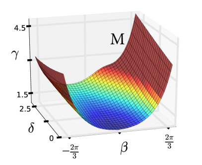
(a)(b)

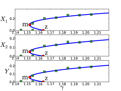
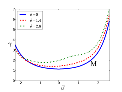
(c) (d)

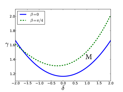
Figure 2: (a) The surface $\mathbf{M}$ depicts the boarder of synchronous states in the parameter space $(\delta,\beta,\gamma)$: above the surface synchrony with $X_{1,2}\neq 0$ and $Y\neq 0$ exists, below only asynchronous state is possible. The internal coupling $\varepsilon=1$ for each population, hence, population are internally asynchronous. (b) The dependence of order parameters on the coupling constant $\gamma$ is shown for $\delta=\beta=0$ and $\varepsilon=1$. The curves denote theoretical calculations using self-consistent scheme, markers correspond to the direct numerical calculations of the finite-size ensemble (10) for $N=8\times 10^{5}$. (c,d) Cuts of the surface $\mathbf{M}$ are shown for constant values of the frequency mismatch $\delta$ (in the panel (c)) and the phase shift $\beta$ (in the panel (d)).

Figure 2(a) shows the area of existence of stationary synchronous solutions in the 3-d parameter space $(\delta,\beta,\gamma)$. The surface $\mathbf{M}$ depicted in the Fig. 2(a) denotes the border of existence of synchronous states: above the surface there exist stationary synchronous solutions with $X_{1,2}\neq 0$ and $Y\neq 0$, below $\mathbf{M}$ only asynchronous state exists and is stable. Figure 2(b) explains the bifurcation diagram depicted in Fig. 2(a), here we fix the parameters $\delta=\beta=0$ and plot order parameters $X_{1,2}$ and $Y$ as a function of parameter $\gamma$ (the latter corresponds to the vertical line passing through the origin in the Fig. 2(a)). As one can see from the plot, there is a minimal critical coupling $\gamma_{cr}$ corresponding to the point $m$ where two branches of synchronous solutions arise. The upper branch appears to be stable, what is confirmed by direct numerical simulation of the finite-size ensemble. The lower branch is unstable and disappears in the point $z$, merging with the trivial state. Apparently, the family of the points $m$ obtained at different values of $\beta$ and $\gamma$ constitutes the surface $\mathbf{M}$ depicted in the Fig. 2(a).

The form of the surface is invariant under transformation $\delta\to-\delta$, $\beta\to-\beta$, that is why only the part with $\delta>0$ is shown in the Fig. 2(a). Expectedly, $\mathbf{M}$ has a global minimum at the point $\delta=\beta=0$ what means that, substantially, phase shift and frequency mismatch act against synchronization. Figures 2(c,d) show several cuts of the surface $\mathbf{M}$ at constant values of $\delta=\text{const}$ (in the panel (c)) and $\beta=\text{const}$ (in the panel (d)). For the most part of the parameter range, the phase shift acts against synchronization, as one can easily see from the Fig. 3(c) where the borders of stationary synchronous states are plotted on the plane $(\beta,\gamma)$. When the frequency mismatch mismatch is absent ($\delta=0$), the curves are symmetric with respect to the line $\beta=0$ and critical coupling increases with growth of the absolute value of $\beta$. However, it is not always a case for non-zero frequency mismatch. The examples for $\delta\neq 0$ in the Fig. 3(c) clearly indicate a nontrivial fact that the global minima of the curves in the $(\beta,\gamma)$ plane are shifted towards negative values of $\beta$. Similarly, on the $(\delta,\gamma)$ the boarder of synchronous states has global minima at non-zero value of $\delta$ for finite phase shift $\beta=\pi/4$.

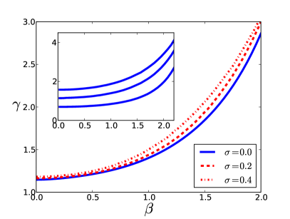
(a)(b)

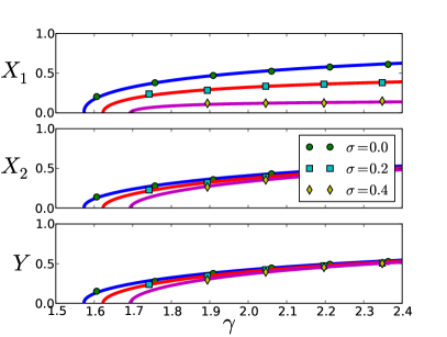
(c)

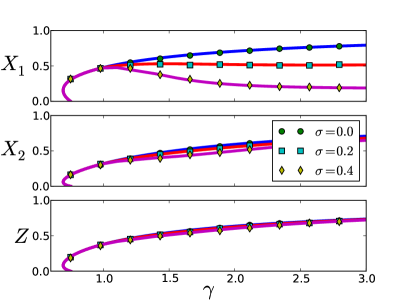
Figure 3: The areas of existence of stationary synchronous solutions on the parameter planes $(\beta,\gamma)$ are shown for the case $\varepsilon=1$ and $\delta=0$. Different curves correspond to boarder of synchronous states with different indicator functions $S(x)=\sigma=\text{const}$ (different multi-branch entrainments). Above the curves solutions with $X_{1,2}\neq 0$, $Y\neq 0$ exist. Inset shows boundaries of synchronous states plotted for different values of constant $\varepsilon$. From bottom to top $\varepsilon=1.5$, $\varepsilon=1.0$, $\varepsilon=0.5$. (b) Dependences of order parameters $X_{1,2}$, $Y$ on cross-coupling $\gamma$ are shown for states with different $\sigma$ (see legend). Solid curves denote solutions of self-consistent equations, markers denote direct calculations of the finite-size ensemble. Other parameters are: $\varepsilon=0.5$, $\beta=0$, $\delta=0$. (c) The same as (b) but for $\varepsilon=1.5$.

Remarkably, the transition to synchrony here is always accompanied by the multiplicity of different synchronous states with multi-branch entrainment (Daido, 1995, 1996b) in the first subpopulation. The issue of multiplicity for the bi-harmonic Kuramoto model was studied in detail in (Komarov and Pikovsky, 2014). The multiple synchronous states appear as a result of strong second harmonic $\sim e^{i2\varphi}$ in a global force acting on oscillators of the first subpopulation. Apparently, in order to get a synchronization in the ensembles due to the cross-coupling, the constant $\gamma$ has to be strong enough, as one can easily see from the bifurcation diagram in Fig. 2(a). The latter implies that the coupling function $h(u,v,\varphi)$ (see eq. (18)) always has a double-well form, hence, there is always a possibility to redistribute oscillators between two stable branches in different ways (in other words, to choose an arbitrary indicator function $S(x)$ in the self-consistent scheme). As a result, for the case of internally asynchronous populations (when $\varepsilon$ is not large enough), a family of synchronous states appears with distinct multi-branch entrainments. Figure 3(a) shows the critical couplings $\gamma$ when synchronous states with distinct redistributions $S(x)$ appear. For the sake of simplicity we chose $S(x)=\sigma=\text{const}$. The dependences of order parameter $X_{1,2}$, $Y$ on the cross-coupling $\gamma$ for different types of multi-branch entrainments (characterized by constant $\sigma$) are presented in the Fig. 2(b). The main state $\sigma=0$ arises first (i.e. at a minimal coupling strengths $\gamma$) in comparison to other states with multi-branch entrainment $\sigma\neq 0$. Expectedly, in all cases increase of the coupling $\gamma$ leads to increase of order parameters values, hence, more oscillators are entrained in both populations.

Here in this section we have concentrated on the effects caused by the cross-coupling $\gamma$ and paid less attention to the role of the internal coupling $\varepsilon$. It is worth mentioning that, in the simplest form (pure sinusoidal coupling) the interaction inside the communities makes a relatively straightforward effect. Namely, increase of the coupling $\varepsilon$ leads to enlargement of the area of synchrony existence in the parameter space (see inset in the Fig. 3).

V Internally synchronous populations: Chaotic dynamics.

In this section we consider the case when $\varepsilon>2$, hence, the populations are internally synchronous even without cross-coupling $\gamma$. Here we report on non-trivial phenomena when resonant cross-coupling introduces chaotic collective oscillations into the system.

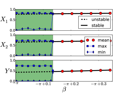
(a)(b)

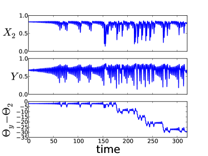
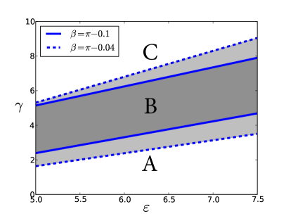
(c)(d)

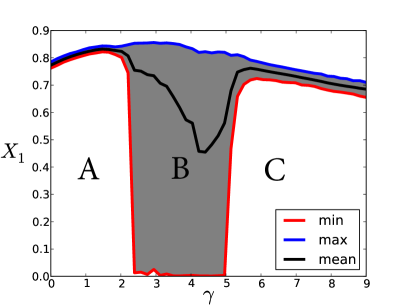
Figure 4: (a) Dependence of order parameters on phase shift $\beta$ is presented. Solid and dashed curves denote solutions obtained from the self-consistent approach. Stable solution corresponds to solid line, unstable to dashed line (stability was checked by direct simulation of the ensemble (10)). Markers correspond to simulation of finite-size ensemble (10) for $N=10^{4}$ oscillators. The colored area denotes chaotic region with large amplitude of order parameters oscillations. Parameters $\varepsilon=4.5$, $\gamma=2.8$. (b) Time series of the finite-size ensembles in the chaotic regime. Parameters: $\varepsilon=4.5$, $\gamma=2.8$, $\beta=-3.0$. (c) The region of existence of chaotic mode on the parameter plane $(\varepsilon,\gamma)$ is presented for $\beta=\pi-0.1$, $\delta=0$. (d) Dependence of the order parameter $X_{1}$ is presented for $\varepsilon=5$, $\beta=\pi-0.1$ and $\delta=0$. The gray area denote maximal amplitude of oscillations obtained from time series after certain transient period.

Figure 4(a) shows the diagram of stationary synchronous states versus phase shift in the cross-coupling function $\beta$. The solid curves correspond to solution obtained from the self-consistent approach above, while markers denote direct numerical calculations of the ensemble (10) at the same parameters. As one can easily see, the stationary states remain stable until $\beta$ is less than certain critical value (indicated by colored area in the Fig. 4(a)). However, when the phase shift becomes relatively close to $\pi$, the synchronous solutions loses stability and immediately the system switches to a chaotic oscillation mode. The corresponding time series is presented in the Fig. 4(b). Remarkably, chaotic oscillations are characterized by a drift of the phase difference $\Theta_{2}-\Theta_{y}$ (see the lowest panel in the Fig. 4(b)), so, the ensembles suddenly become unlocked from each other when entering to chaotic mode.

Fig. 4(c) is aimed to explain the structure of parameter area where chaotic mode exists. As one can see, for each sufficiently strong internal coupling $\varepsilon$, there is always a certain range of cross-coupling constant $\gamma$, where oscillations are irregular. With an increase of the cross-coupling $\gamma$, the system pass from area $A$ (the area where regular synchronous solution exists) to area $B$ which corresponds to chaotic motion. As has been mentioned above, area $B$ is characterized by a drift of the phase difference and large amplitude irregular oscillations of the order parameters (see Fig. 4(d)). Further increase of constant $\gamma$ leads back to a regular stationary synchronous solution (Fig. 4(d)). The size of the area $B$ on the $(\varepsilon,\gamma)$ plane is strongly related to the phase shift in coupling function: the closer the parameter $\beta$ to $\pi$, the larger the area $B$ on the $(\varepsilon,\gamma)$ plane.

VI Conclusions

The phase reduction is one of the few mathematical techniques which allows one to perform analytical studies of complex nonlinear oscillatory systems. Perhaps, the most popular and well-studied phase model is the classical Kuramoto system which describes ensemble of globally coupled oscillators with sinusoidal type of interaction function. The derivation of various Kuramoto-type models is based on the assumption of closeness of natural oscillatory frequencies. However, in many realistic situations oscillators may have definitely different frequencies; an example of this are neural populations that can produce brain waves wide across the spectrum. For multifrequency populations one has to extend typical model of phase equations; in previously considered cases such an extension also led to new dynamical regimes (Komarov and Pikovsky, 2013b, 2011).

In the present paper we developed an extension of the phase synchronization theory for multifrequency resonant oscillator communities. After analysing general possible resnonant terms in linear mean-field coupling, we focused on the simplest high-order resonant case, when two communities of oscillators are globally coupled and have natural population frequencies close to the rational relation 2:1. First, given the assumption on mean population frequencies, we derived the simplest form of phase equations for high-order resonant interaction between two globally coupled communities of oscillators. Basically, the structure of the model consists of two main parts: the first part represents classical sinusoidal term describing Kuramoto-type interaction inside each community; the second component has different form, it represents the resonant cross- coupling between the populations. Next, we combine two approaches described in Refs. Komarov and Pikovsky (2013a); *Komarov-Pikovsky-14 and in Refs. Ott and Antonsen (2008); *Ott-Antonsen-09 to derive a self- consistent scheme for calculation of stationary synchronous solutions of the system in the thermodynamical limit.

In this paper we focused on investigation how cross-coupling promotes synchronization, and looked for novel dynamical effects due to the high-order resonance. Hence, we have considered two qualitatively different cases, in the first case the populations were internally asynchronous, so, the internal coupling strength was relatively weak. Here we constructed the bifurcation diagram showing how synchronous regimes appear in dependence on main parameters of the model. We demonstrated, that strong enough resonant cross-coupling results in stationary synchronous solutions appearing in both subpopulations. Thus, the synchrony can be only mutual. The nontrivial fact here is that the transition to synchrony due to the cross-coupling is always accompanied by multiplicity of distinct synchronous states, similar to the case of bi- harmonic Kuramoto model Komarov and Pikovsky (2013a); *Komarov-Pikovsky-14. In the second setup, we considered an opposite situation, when the internal coupling is strong, such that almost all oscillators are locked to the mean fields in the absence of the cross- coupling. Here we report on a quite non-trivial effect, that the cross-coupling can destroy the stationary synchronous state introducing chaos into the system. Mean fields of two subpopulations not only vary their amplitude chaotically, but the subpopulations also desynchronize from each other in the sense, that the phase shift between the mean fields is no more a constant, but performs a biased random walk.

VII Acknowledgement

M. K. thanks Alexander von Humboldt Foundation for support. The research in sections IV and V was supported by the Russian Science Foundation (Project 14-12-00811).

References

- Wiesenfeld and Swift (1995) K. Wiesenfeld and J. W. Swift, Phys. Rev. E 51, 1020 (1995).
- Wiesenfeld et al. (1996) K. Wiesenfeld, P. Colet, and S. H. Strogatz, Phys. Rev. Lett. 76, 404 (1996).
- Wiesenfeld et al. (1998) K. Wiesenfeld, P. Colet, and S. Strogatz, Physical Review E 57, 1563 (1998).
- Kiss et al. (2002) I. Kiss, Y. Zhai, and J. Hudson, Science 296, 1676 (2002).
- Grollier et al. (2006) J. Grollier, V. Cros, and A. Fert, Phys. Rev. B 73, 060409(R) (2006).
- Georges et al. (2008) B. Georges, J. Grollier, V. Cros, and A. Fert, Appl. Phys. Lett. 92, 232504 (2008).
- Golomb et al. (2001) D. Golomb, D. Hansel, and G. Mato, in Neuro-informatics and Neural Modeling, Handbook of Biological Physics, Vol. 4, edited by F. Moss and S. Gielen (Elsevier, Amsterdam, 2001) pp. 887–968.
- Breakspear et al. (2010) M. Breakspear, S. Heitmann, and A. Daffertshofer, Frontiers in human neuroscience 4, 190 (2010).
- Gonze et al. (2005) D. Gonze, S. Bernard, C. Waltermann, A. Kramer, and H. Herzel, Biophysical Journal 89, 120 (2005).
- Bordyugov et al. (2013) G. Bordyugov, P. Westermark, A. Korencic, and H. Herzel, in Circadian Clocks, edited by A. Kramer and M. Merrow (Springer, 2013).
- Eckhardt et al. (2007) B. Eckhardt, E. Ott, S. H. Strogatz, D. M. Abrams, and A. McRobie, Phys. Rev. E 75, 021110 (2007).
- Néda et al. (2000) Z. Néda, E. Ravasz, T. Vicsek, Y. Brechet, and A. L. Barabási, Phys. Rev. E 61, 6987 (2000).
- Kuramoto (1984) Y. Kuramoto, Chemical Oscillations, Waves and Turbulence (Springer, Berlin, 1984).
- Pikovsky et al. (2001) A. Pikovsky, M. Rosenblum, and J. Kurths, Synchronization. A Universal Concept in Nonlinear Sciences. (Cambridge University Press, Cambridge, 2001).
- Kuramoto (1975) Y. Kuramoto, in International Symposium on Mathematical Problems in Theoretical Physics, edited by H. Araki (Springer Lecture Notes Phys., v. 39, New York, 1975) p. 420.
- Izhikevich (2007) E. M. Izhikevich, Dynamical Systems in Neuroscience (MIT Press, Cambridge, Mass., 2007).
- Izhikevich (2000) E. M. Izhikevich, SIAM Journal on Applied Mathematics 60, 1789 (2000).
- Daido (1993a) H. Daido, Physica D 69, 394 (1993a).
- Daido (1993b) H. Daido, Prog. Theor. Phys. 89, 929 (1993b).
- Daido (1996a) H. Daido, Physica D 91, 24 (1996a).
- Daido (1995) H. Daido, J. Phys. A: Math. Gen. 28, L151 (1995).
- Acebrón et al. (2005) J. A. Acebrón, L. L. Bonilla, C. J. P. Vicente, F. Ritort, and R. Spigler, Rev. Mod. Phys. 77, 137 (2005).
- Watanabe and Strogatz (1994) S. Watanabe and S. H. Strogatz, Physica D 74, 197 (1994).
- Ott and Antonsen (2008) E. Ott and T. M. Antonsen, CHAOS 18, 037113 (2008).
- Ott and Antonsen (2009) E. Ott and T. M. Antonsen, CHAOS 19, 023117 (2009).
- Marvel et al. (2009) S. A. Marvel, R. E. Mirollo, and S. H. Strogatz, Chaos 19, 043104. (2009).
- Pikovsky and Rosenblum (2008) A. Pikovsky and M. Rosenblum, Phys. Rev. Lett. 101, 264103 (2008).
- Pikovsky and Rosenblum (2011) A. Pikovsky and M. Rosenblum, Physica D 240, 872 (2011).
- Omel’chenko and Wolfrum (2012) O. E. Omel’chenko and M. Wolfrum, Phys. Rev. Lett. 109, 164101 (2012).
- Omel’chenko and Wolfrum (2013) O. E. Omel’chenko and M. Wolfrum, Physica D 263, 74 (2013).
- Daido (1996b) H. Daido, Phys. Rev. Lett. 77, 1406 (1996b).
- Crawford (1995) J. D. Crawford, Phys. Rev. Lett. 74, 4341 (1995).
- Crawford and Davies (1999) J. D. Crawford and K. T. R. Davies, Physica D 125, 1 (1999).
- Chiba and Nishikawa (2011) H. Chiba and I. Nishikawa, Chaos 21, 043103 (2011).
- Hansel et al. (1993) D. Hansel, G. Mato, and C. Meunier, Phys. Rev. E 48, 3470 (1993).
- Ashwin et al. (2007) P. Ashwin, G. Orosz, J. Wordsworth, and S. Townley, SIAM Journal on Applied Dynamical Systems 6, 728 (2007).
- Komarov and Pikovsky (2013a) M. Komarov and A. Pikovsky, Phys. Rev. Lett. 111, 204101 (2013a).
- Komarov and Pikovsky (2014) M. Komarov and A. Pikovsky, Physica D 289, 18 (2014).
- Vlasov et al. (2015) V. Vlasov, M. Komarov, and A. Pikovsky, J. Phys. A: Mathematical and Theoretical 48, 105101 (2015).
- Lück and Pikovsky (2011) S. Lück and A. Pikovsky, Physics Letters A 375, 2714 (2011).
- Komarov and Pikovsky (2013b) M. Komarov and A. Pikovsky, Phys. Rev. Lett. 110, 134101 (2013b).
- Komarov and Pikovsky (2011) M. Komarov and A. Pikovsky, Phys. Rev. E 84, 016210 (2011).
- Buzsáki (2006) G. Buzsáki, Rhythms of the brain (Oxford UP, Oxford, 2006).
- Rosjat et al. (2014) N. Rosjat, S. Popovych, and S. Daun-Gruhn, Theoretical Biology and Medical Modelling 11 (2014).
- Komarov et al. (2014) M. Komarov, S. Gupta, and A. Pikovsky, EPL 106, 40003 (2014).