The Parametric Frobenius Problem

Abstract

Given relatively prime positive integers $a_{1},\ldots,a_{n}$, the Frobenius number is the largest integer that cannot be written as a nonnegative integer combination of the $a_{i}$. We examine the parametric version of this problem: given $a_{i}=a_{i}(t)$ as functions of $t$, compute the Frobenius number as a function of $t$. A function $f:\mathbb{Z}_{+}\rightarrow\mathbb{Z}$ is a quasi-polynomial if there exists a period $m$ and polynomials $f_{0},\ldots,f_{m-1}$ such that $f(t)=f_{t\bmod m}(t)$ for all $t$. We conjecture that, if the $a_{i}(t)$ are polynomials (or quasi-polynomials) in $t$, then the Frobenius number agrees with a quasi-polynomial, for sufficiently large $t$. We prove this in the case where the $a_{i}(t)$ are linear functions, and also prove it in the case where $n$ (the number of generators) is at most 3.

1 Introduction

Given positive integers $a_{i}$, $1\leqslant i\leqslant n$, let

$$\left\langle{a_{1},\ldots,a_{n}}\right\rangle=\left\{\vphantom{x^{2}}{\sum_{i=1}^{n}p_{i}a_{i}}\,\middle|\,{p_{i}\in\mathbb{Z}_{\geqslant 0}}\right\}$$

be the semigroup generated by the $a_{i}$. If the $a_{i}$ are relatively prime, define the Frobenius number $F(a_{1},\ldots,a_{n})$ to be the largest integer not in $\left\langle{a_{1},\ldots,a_{n}}\right\rangle$. The Frobenius problem of determining $F(a_{1},\ldots,a_{n})$ has a long history — Sylvester proved [8] in 1884 that $F(a,b)=ab-a-b$, and see Ramírez Alfonsín’s book [5] for many subsequent results.

It will be convenient to also define $F(a_{1},\ldots,a_{n})$ in the case where the $a_{i}$ are not relatively prime, so that there is no largest integer not in the semigroup. A reasonable definition seems to be the largest integer in the group $\mathbb{Z}a_{1}+\cdots+\mathbb{Z}a_{n}$ that is not in the semigroup $\left\langle{a_{1},\ldots,a_{n}}\right\rangle$. That is, if $d$ is the greatest common divisor of $a_{1},\ldots,a_{n}$, then $F(a_{1},\ldots,a_{n})=dF(\frac{a_{1}}{d},\ldots,\frac{a_{n}}{d})$. Sylvester’s identity then becomes $F(a,b)=\operatorname{lcm}(a,b)-a-b$.

The parametric Frobenius problem is, given functions $a_{i}:\mathbb{Z}_{+}\rightarrow\mathbb{Z}_{+}$ to determine $F\big{(}a_{1}(t),\ldots,a_{n}(t)\big{)}$ as a function of $t$. For example, using Sylvester’s identity,

$$F(t,t+2)=\begin{cases}t(t+2)-t-(t+2)&\text{if $t$ is odd,}\\ \frac{t(t+2)}{2}-t-(t+2)&\text{if $t$ is even.}\end{cases}$$

We see that $F(t,t+2)$ is a quasi-polynomial; a function $f:\mathbb{Z}_{+}\rightarrow\mathbb{Z}$ is a quasi-polynomial if there exist an $m\in\mathbb{Z}_{+}$ and polynomials $f_{0},\ldots,f_{m-1}\in{\mathbb{Q}}[t]$ such that $f(t)=f_{t\bmod m}(t)$ for all $t\in\mathbb{Z}_{+}$. Here $m$ is a period of $f$ and the $f_{i}$ are components of $f$. We will assume that all of our functions are integer-valued, but note that the $F(t,t+2)$ example shows that we may need polynomials with rational coefficients.

In general, our functions may misbehave for small $t$. We say that a property is eventually true if it is true for all sufficiently large $t$. We say that $f(t)\in\operatorname{EQP}$ (short for eventual quasi-polynomial) if $f(t)$ eventually agrees with a quasi-polynomial. We say that the degree of $f\in\operatorname{EQP}$ is the maximum degree of its components.

We conjecture that, if $a_{i}(t)\in\operatorname{EQP}$, then $F\big{(}a_{1}(t),\ldots,a_{n}(t)\big{)}\in\operatorname{EQP}$. We prove this for the special case where the $a_{i}(t)$ are linear functions and for the special case where $n\leqslant 3$.

Conjecture 1.1.

Suppose that $a_{i}(t)\in\operatorname{EQP}$, $1\leqslant i\leqslant n$, are eventually positive. Then $F\big{(}a_{1}(t),\ldots,a_{n}(t)\big{)}\in\operatorname{EQP}$.

Theorem 1.2.

Suppose that $a_{i}(t)\in\operatorname{EQP}$, $1\leqslant i\leqslant n$, are eventually positive and have degree at most 1. Then $F\big{(}a_{1}(t),\ldots,a_{n}(t)\big{)}\in\operatorname{EQP}$, with degree at most 2.

Theorem 1.3.

Suppose that $a_{i}(t)\in\operatorname{EQP}$, $1\leqslant i\leqslant n$, are eventually positive, with $n\leqslant 3$. Then $F\big{(}a_{1}(t),\ldots,a_{n}(t)\big{)}\in\operatorname{EQP}$.

These results are examples of so-called “unreasonable” appearances of quasi-polynomials, as discussed by Woods [10]. “Reasonable” appearances trace back to Ehrhart’s classical result [3] that, if $P\subseteq\mathbb{R}^{n}$ is a polytope with rational vertices, then $f(t)=\#(tP\cap\mathbb{Z}^{n})$ is a quasi-polynomial. Note that if $P$ is defined with linear inequalities $\mathbf{b}_{i}\cdot\mathbf{x}\leqslant c_{i}$, then $tP$ is defined with linear inequalities $\mathbf{b}_{i}\cdot\mathbf{x}\leqslant c_{i}t$. As $t$ changes, these linear inequalities move, but their normal vectors ($\mathbf{b}_{i}$) remain the same. Indeed, Woods proved [11] that any example over the integers defined with linear inequalities, boolean operations (and, or, not), and quantifiers ($\forall$, $\exists$) has this quasi-polynomial behavior. This is true even if there is more than one parameter; for example,

$$\#\left\{\vphantom{x^{2}}{(x,y)\in\mathbb{Z}^{2}_{\geqslant 0}}\,\middle|\,{2x\leqslant t,\,3y\leqslant s}\right\}=\bigg{(}\left\lfloor\frac{t}{2}+1\right\rfloor\bigg{)}\bigg{(}\left\lfloor\frac{s}{3}+1\right\rfloor\bigg{)}$$

is a quasi-polynomial of period 2 in $t$ and period 3 in $s$.

If we look at the parametric Frobenius problem, however, we see that it does not fit this pattern. For example, if we want to ask whether $u\in\left\langle{t,t+1,t+2}\right\rangle$, we are asking whether the polytope

$$\left\{\vphantom{x^{2}}{(x,y,z)\in\mathbb{R}^{3}_{\geqslant 0}}\,\middle|\,{u=tx+(t+1)y+(t+2)z}\right\}$$

contains any integer points. For a fixed $t$, this is a 2-dimensional triangle in $\mathbb{R}^{3}$; as $t$ changes, this triangle “twists” (the normal vector changes). Examples such as this were categorized in [10] as “unreasonable”, though they are conjectured to still lead to eventual quasi-polynomial behavior.

This paper adds a third example to the list of recent results demonstrating this phenomenon; previously Chen, Li, and Sam [2] showed that the number of integer points in a polytope whose vertices are rational functions of $t$ is in $\operatorname{EQP}$, and Calegari and Walker [1] showed that the vertices of the integer hull of such a polytope have coordinates in $\operatorname{EQP}$. A critical tool used in all of these results is that the division algorithm and the gcd of polynomials has quasi-polynomial behavior (cf. Lemma 3.1); for example, the Euclidean algorithm yields

$$\gcd(2t+1,5t+6)=\gcd(t+4,2t+1)=\gcd(7,t+4)=\begin{cases}7&\text{if $t\equiv 3\bmod 7$,}\\ 1&\text{otherwise.}\end{cases}$$

Note that unlike in the “reasonable” case, these results only hold with one parameter variable. For example $F(s,t)=\operatorname{lcm}(s,t)-s-t$ is not a quasi-polynomial in $s$ and $t$.

The original inspiration for this paper comes from a conjecture of Wagon [9] (see [4, Section 17]) that, for any fixed $M$ and residue class $j$ of $t\bmod M^{2}$, there exist (usually positive) integers $c_{M,j}$ and $d_{M,j}$ such that eventually

$$F(t,t+1^{2},t+2^{2},\ldots,t+M^{2})=\frac{1}{M^{2}}\left(t^{2}+c_{M,j}t\right)-d_{M,j}.$$

Using the proof of Theorem 1.2, we can prove that there is indeed quasi-polynomial behavior with period $M^{2}$. In fact, such a result holds in greater generality:

Corollary 1.4.

Suppose $b_{1}<b_{2}<b_{3}<\cdots<b_{n}$ are integers. Then $F(t+b_{1},t+b_{2},\ldots,t+b_{n})\in\operatorname{EQP}$ with period $b_{n}-b_{1}$.

When the $b_{i}$ form an arithmetic sequence, a precise quasi-polynomial formula was previously given by Roberts [6]:

$$F(t,t+d,\ldots,t+sd)=\left(\left\lfloor\frac{t-2}{s}\right\rfloor+1\right)t+(d-1)(t-1)-1.$$

In Section 2, we work through the example

$$F(t,t+1,t+2)=\left(\left\lfloor\frac{t-2}{2}\right\rfloor+1\right)t-1=\begin{cases}\frac{t^{2}}{2}&\text{if $t$ even,}\\ \frac{t^{2}}{2}-\frac{t}{2}-1&\text{if $t$ odd,}\end{cases}$$

which will give a flavor of our general proof. In Section 3, we prove Theorem 1.2. In Section 4, we prove the various lemmas needed. In Section 5, we prove Corollary 1.4. In Section 6, we prove Theorem 1.3, using Rødseth’s algorithm [7] for the 3 generator Frobenius problem.

The proof of Theorem 1.2 relies on the fact that semigroups with only two generators are much easier to deal with. Indeed, we have the following definition and lemma:

Definition 1.5.

Let $a,b\in\mathbb{Z}_{+}$ be relatively prime, and let $c\in\mathbb{Z}$. The canonical form for $c$ is given by $c=pa+qb$ with $p,q\in\mathbb{Z}$ and $0\leqslant p<b$.

Lemma 1.6.

Let $a,b\in\mathbb{Z}_{+}$ be relatively prime, and let $c\in\mathbb{Z}$.

1. The canonical form for $c$ exists and is unique. In particular, if $c=p^{\prime}a+q^{\prime}b$ is any form with $p^{\prime},q^{\prime}\in\mathbb{Z}$, and if $k$ and $r$ are the quotient and remainder when $p^{\prime}$ is divided by $b$, then the canonical form for $c$ is $ra+(q^{\prime}+ka)b$.

2. If $c=pa+qb$ is in canonical form, $c\in\left\langle{a,b}\right\rangle$ if and only if $q\geqslant 0$.

2 An Example

In this example, we compute $F(t,t+1,t+2)$. Let $a=t$, $b=t+1$, and $c=t+2$ be our three generators, let $S=\left\langle{a,b,c}\right\rangle$, and let $T=\left\langle{a,c}\right\rangle$. Notice that $2b=a+c$. This implies that $S=T\cup(b+T)$, as follows: if $pa+qb+rc$ is a representation of an element of $S$, with $p,q,r\in\mathbb{Z}_{\geqslant 0}$ and $q\geqslant 2$, then $(p+1)a+(q-2)b+(r+1)c$ is also a representation, so we may assume without loss of generality that $q$ is $0$ or $1$ (cf. Lemma 3.4). Next, we run the extended Euclidean algorithm on the integers $a$ and $c$, and get

$$\gcd(a,c)=\gcd(t,t+2)=\gcd(2,t)$$

(cf. Lemma 3.1). The next division step in the algorithm depends on the parity of $t$, and rather than end up with the messy $\left\lfloor t/2\right\rfloor$, we divide into two cases.

$\boldsymbol{\text{The case }t\text{ is odd}}$: Let $t=2s+1$, so that $a=2s+1$, $b=2s+2$, and $c=2s+3$. Now

$$\gcd(a,c)=\gcd(2,2s+1)=\gcd(1,2)=1,$$

and the extended Euclidean algorithm yields $1=(s+1)a-sc$. Let $u\in\mathbb{Z}$, and we are wondering whether $u\notin S$, that is, $u\notin T$ and $u\notin b+T$. Suppose that

$$u=pa+qc$$

is the canonical form for $u$ (see Definition 1.5). Lemma 1.6(2) tells us that $u\in T$ if and only if $q\geqslant 0$. Since we are looking for $u\notin T$, we may assume from here on out that $q<0$. To characterize when $u\in b+T$ (that is, $u-b\in T$) we must find the canonical form for $u-b$.

First we compute the canonical form for $b$. Multiplying the equation $1=(s+1)a-sc$ by $b=2s+2$ yields some form for $b$:

$$b=(2s+2)(s+1)a-(2s+2)sc.$$

By Lemma 1.6(1), we may find the canonical form by dividing $(2s+2)(s+1)$ by $c=2s+3$: the quotient is $s$ with remainder $s+2$, giving the canonical form for $b$ as

$$b=(s+2)a-sc.$$

Note that we got a little lucky here: our remainder of $s+2$ is clearly less than $c=2s+3$; if our remainder had instead been $s+7$, say, then we would only have the canonical form for sufficiently large $s$.

Now we have that some form for $u-b$ is

$$u-b=(p-s-2)a+(q+s)c.$$

Is this the canonical form? There are two cases:

If $p\geqslant s+2$, then $0\leqslant p-s-2\leqslant p<c$, and this is in canonical form. Therefore, to have $u-b\in T$, we must have $q+s\geqslant 0$ (again using Lemma 1.6(2)), that is, $q\geqslant-s$.

If $p<s+2$, then the canonical form is

$$u-b=(p-s-2+c)a+(q+s-a)c=(p+s+1)a+(q-s-1)c$$

(to check that this is canonical, note that $p\geqslant 0$ and $s+2<c$ imply $p-s-2+c\geqslant 0$, and $p<s+2$ implies $p-s-2+c<c$). In this case, to have $u-b\in T$, we must have $q\geqslant s+1$. This implies that $q\geqslant 0$, but we have assumed $q<0$ (so that $u\notin T$). Therefore this case never has $u-b\in T$.

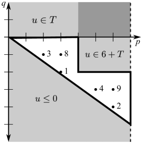
Figure 1: The $t=5$ case of the example. We have $T=\left\langle{5,7}\right\rangle$ and $S=\left\langle{5,6,7}\right\rangle=T\cup(6+T)$. Points $(p,q)\in\mathbb{Z}^{2}$ with $0\leqslant p<7$ are the canonical forms for $u=5p+7q\in\mathbb{Z}$. Then $q\geqslant 0$ corresponds to $u\in T$, $(p,q)\geqslant(4,-2)$ corresponds to $u\in 6+T$, and positive $u$ such that $u\notin S$ are labelled beside their corresponding $(p,q)$. The “corners” $u=8$ and $u=9$ are candidates for the Frobenius number, and so $F(5,6,7)=\max\{8,9\}=9$.

To summarize across both cases, if $u=pa+qc$, with $0\leqslant p<c=2s+3$ in the canonical form, then $u\notin S$ if and only if

$$\text{not}(q\geqslant 0)\quad\text{and}\quad\text{not}\big{(}(p,q)\geqslant(s+2,-s)\big{)}$$

(cf. Lemma 3.5). The set of such $(p,q)$ has a “stairstep” shape, as can be seen in Figure 1 for $t=5$. In particular, the set of such $(p,q)$ can be rewritten as $p\geqslant 0$ and

$$\big{(}p\leqslant s+1\quad\text{and}\quad q\leqslant-1\big{)}\quad\text{or}\quad\big{(}p\leqslant 2s+2\quad\text{and}\quad q\leqslant-s-1\big{)}$$

(cf. proof of Lemma 3.6, $d=1$ case). The two “corners” in this picture, where both inequalities of one of these two conjunctions are tight, give our candidates for the largest $u\notin S$: it must be either

$$(s+1)a-1c=2s^{2}+s-2\quad\text{or}\quad(2s+2)a+(-s-1)c=2s^{2}+s-1.$$

The latter is always larger (in general, one might only be eventually larger than the other), and so we have

$$F(t,t+1,t+2)=2s^{2}+s-1=\frac{t^{2}}{2}-\frac{t}{2}-1,$$

in this case where $t=2s+1$ is odd.

$\boldsymbol{\text{The case }t\text{ is even}}$: Let $t=2s$, so that $a=2s$, $b=2s+1$, and $c=2s+2$. To have $u\notin S$ we must have both $u\notin T=\left\langle{a,c}\right\rangle$ and $u\notin b+T$. Note that every element in $T$ is even and every element of $b+T$ is odd. Therefore the largest even integer not in S is the largest even integer not in $T$, which since $T$ has only 2 generators is simply $\operatorname{lcm}(a,c)-a-c=2s^{2}-2s-2$ (we’re getting lucky here that we didn’t have to do an analysis similar to the $t$ is odd case). Similarly the largest odd integer not in $S$ is the largest odd integer not in $b+T$, which is $b+(2s^{2}-2s-2)=2s^{2}-1$. The largest integer not in $S$ is then the maximum of these two candidates, so $F(t,t+1,t+2)=2s^{2}-1=\frac{t^{2}}{2}-1$ (cf. proof of Lemma 3.6, $d>1$ case), in this case where $t$ is even.

Combining the even and odd case, we have proved that

$$F(t,t+1,t+2)=\begin{cases}\frac{t^{2}}{2}&\text{if $t$ even,}\\ \frac{t^{2}}{2}-\frac{t}{2}-1&\text{if $t$ odd.}\end{cases}$$

3 Proof of Theorem 1.2

This first lemma gives us the basic tools we need:

Lemma 3.1.

Given $f,g\in\operatorname{EQP}$,

1. There exists an $m\in\mathbb{Z}_{+}$ such that, for each $0\leqslant j<m$, $f(ms+j)$ eventually agrees with a polynomial in $\mathbb{Z}[s]$.

2. If $\deg(g)>0$, there exists $q,r\in\operatorname{EQP}$ such that $f(t)=q(t)g(t)+r(t)$ and $\deg(r)<\deg(g)$. Note that this is the analogue of the traditional division algorithm over ${\mathbb{Q}}[t]$.

3. If $g(t)$ is eventually positive, there exists $q,r\in\operatorname{EQP}$ such that $f(t)=q(t)g(t)+r(t)$ and eventually $0\leqslant r(t)<g(t)$. Furthermore, $\deg(r)\leqslant\deg(g)$. Note that this is the analogue of the traditional division algorithm over $\mathbb{Z}$.

4. There exists $p,q,d\in\operatorname{EQP}$ such that $\gcd\big{(}f(t),g(t)\big{)}=d(t)$ and $d(t)=p(t)f(t)+q(t)g(t)$.

5. We have $\max\big{(}f(t),g(t)\big{)}\in\operatorname{EQP}$.

These are proved in Section 4 of [2] (and also in [1]), so in Section 4 we merely give an outline of the important steps.

Remark 3.2.

Lemma 3.1(1) will allow us to often simply say “without loss of generality, $f\in\mathbb{Z}[t]$”: we may analyze $f(ms+j)$ for each $j$, recognize that statements may be false for small $s$, and then convert back to $t$ using $s=(t-j)/m$.

Using this remark, we may assume that the $a_{i}(t)$ are polynomials in $\mathbb{Z}[t]$. Since they are of degree at most 1 and eventually positive, we have that

$$a_{i}(t)=\alpha_{i}t+\beta_{i},$$

with either $\alpha_{i}\in\mathbb{Z}_{+}$, $\beta_{i}\in\mathbb{Z}$ or $\alpha_{i}=0$, $\beta_{i}\in\mathbb{Z}_{+}$. Furthermore, without loss of generality, we may assume that they are ordered so that

$$\beta_{i}\alpha_{j}\leqslant\beta_{j}\alpha_{i}$$

for $i\leqslant j$, that is (for $\alpha_{i}\neq 0$),

$$\frac{\beta_{1}}{\alpha_{1}}\leqslant\frac{\beta_{2}}{\alpha_{2}}\leqslant\cdots\leqslant\frac{\beta_{n}}{\alpha_{n}}.$$

We first consider a degenerate case, where $\beta_{i}\alpha_{j}=\beta_{j}\alpha_{i}$, for all $i,j$.

Lemma 3.3.

If $\beta_{i}\alpha_{j}=\beta_{j}\alpha_{i}$, for all $i,j$, then there are $\alpha_{0},\beta_{0}\in\mathbb{Z}_{\geqslant 0}$ such that, for all $i$, $\alpha_{i}=\gamma_{i}\alpha_{0}$ and $\beta_{i}=\gamma_{i}\beta_{0}$ (for some $\gamma_{i}\in\mathbb{Z}_{+}$). Therefore

$$F\big{(}a_{1}(t),\ldots,a_{n}(t)\big{)}=F(\gamma_{1},\ldots,\gamma_{n})\cdot(\alpha_{0}t+\beta_{0})$$

is a polynomial of degree at most 1.

Therefore, we can assume that $\beta_{1}\alpha_{n}<\beta_{n}\alpha_{1}$. In particular, the polynomials $a_{1}$ and $a_{n}$ do not share a linear factor, and so if $d(t)=\gcd\big{(}a_{1}(t),a_{n}(t)\big{)}$, then $d(t)\in\operatorname{EQP}$ is of degree 0, that is, $d(t)$ is eventually a periodic function. Let $S(t)=\left\langle{a_{1}(t),\ldots,a_{n}(t)}\right\rangle$, and let $T(t)=\left\langle{a_{1}(t),a_{n}(t)}\right\rangle$. $T(t)$ is a semigroup with only two generators, so it is much easier to analyze. The following lemma allows us to cover $S(t)$ with a finite number of translated copies of $T(t)$.

Lemma 3.4.

For $a_{i}(t)=\alpha_{i}t+\beta_{i}$ as described above, there exists a finite set $H$ of integer-valued polynomials of degree at most 1 such that

$$\left\langle{a_{1}(t),\ldots,a_{n}(t)}\right\rangle=\bigcup_{h\in H}\Big{(}h(t)+\left\langle{a_{1}(t),a_{n}(t)}\right\rangle\Big{)}$$

(for $t$ sufficiently large so that $a_{i}(t)>0,\forall i$). Furthermore, $0\in H$ and the other $h\in H$ are eventually positive.

Assume for the moment that $a_{1}(t)$ and $a_{n}(t)$ are relatively prime. By Lemma 1.6(2), the set of all integers not in $T$ will be in bijection to the set

$$\left\{\vphantom{x^{2}}{(p,q)\in\mathbb{Z}^{2}}\,\middle|\,{0\leqslant p<a_{n}(t),\,q<0}\right\},$$

under the bijection $(p,q)\mapsto pa_{1}(t)+qa_{n}(t)$. By Lemma 3.4, integers not in $S$ must also not be in $h(t)+T$, for all $h\in H$. The following lemma gives an easy way to check this.

Lemma 3.5.

Let $f,g,h\in\operatorname{EQP}$, with $f(t)$ and $g(t)$ relatively prime for all $t$ and with $f(t),g(t),h(t)$ eventually positive. There exists $r,s\in\operatorname{EQP}$ such that, given $p,q\in\mathbb{Z}$ with $0\leqslant p<g(t)$ and $q<0$,

$$pf(t)+qg(t)\in h(t)+\left\langle{f(t),g(t)}\right\rangle\quad\text{if and only if}\quad(p,q)\geqslant\big{(}r(t),s(t)\big{)}$$

component-wise. Furthermore, $\deg(r)\leqslant\deg(g)$ and $\deg(s)\leqslant\max\{\deg(f),\deg(h)-\deg(g)\}$,

In our case, this gives $r,s$ of degree at most 1. If $a_{1}(t)$ and $a_{n}(t)$ are relatively prime, all that remains is to follow the implications of Lemmas 3.4 and Lemma 3.5, which will give us a staircase-shaped set such as in Figure 1. If $a_{1}(t)$ and $a_{n}(t)$ are not relatively prime, we must reduce to the case where they are. Both of these are accomplished in the following lemma, which (combined with Lemma 3.4 and the fact that $d(t)=\gcd\big{(}f(t),g(t)\big{)}$ is of degree 0) proves our theorem.

Lemma 3.6.

Let $f(t),g(t)\in\operatorname{EQP}$, and let $d(t)=\gcd\big{(}f(t),g(t)\big{)}$ be of degree 0, let $H\subseteq\operatorname{EQP}$ be a finite set, and let

$$S(t)=\bigcup_{h\in H}\big{(}h(t)+\left\langle{f(t),g(t)}\right\rangle\big{)}.$$

The function $F(t)$ giving the largest integer not in $S(t)$ is in $\operatorname{EQP}$, with degree at most $\max\{\deg(f)+\deg(g),\deg(h)\}$.

In our case, this gives that $F$ is of degree at most 2.

4 Proofs of Lemmas

Proof of Lemma 1.6.

Part 1 is a standard result, using the extended Euclidean algorithm and the fact that if $c=p^{\prime}a+q^{\prime}b$ is one solution, then all solutions are given by $c=(p^{\prime}-kb)a+(q^{\prime}+ka)b$ for $k\in\mathbb{Z}$.

For part 2, we have $c=pa+qb$ with $0\leqslant p<b$. The reverse implication is immediate: if $q\geqslant 0$, then we have written $c=pa+qb$ with $p,q\in\mathbb{Z}_{\geqslant 0}$, proving that $c\in\left\langle{a,b}\right\rangle$. Conversely, suppose $c\in\left\langle{a,b}\right\rangle$ so that $c=p^{\prime}a+q^{\prime}b$ with $p^{\prime},q^{\prime}\in\mathbb{Z}_{\geqslant 0}$. By part 1, if $k$ and $r$ are the quotient and remainder when $p^{\prime}$ is divided by $b$, then

$$c=ra+(q^{\prime}+ka)b$$

is the canonical form for c, with $q=q^{\prime}+ka\geqslant 0$. ∎

Proof of Lemma 3.1.

As these are proved in Section 4 of [2], we simply give an outline here.

For part 1, this is mostly obvious: simply take component polynomials of the quasi-polynomial. The main subtlety, as seen in the example from Section 2, is that integer-valued polynomials may have non-integral coefficients. In this case, let $m$ be the least common multiple of the denominators of the coefficients. Examining $f(ms+i)$, we see that all coefficients of $s^{k}$ must be integral, except possibly the constant coefficient; since the function is integer-valued, the constant coefficient must also be integral.

For part 2, simply perform polynomial division. The main subtlety is the following: Suppose, for example, that $f(t)=t^{2}+3t$ and $g(t)=2t+1$. Then the leading coefficient of $g$ does not divide the leading coefficient of $f$, and the traditional polynomial division algorithm would produce quotients that are not integer-valued. Instead, we look separately at each residue class of $t$ modulo the leading coefficient of $g$; for example, if $t$ is odd, then $t=2s+1$ for some $s\in\mathbb{Z}_{\geqslant 0}$, so substituting gives $f(2s+1)=4s^{2}+10s+3$ and $g(2s+1)=4s+3$, and now the leading term does divide evenly.

For part 3, first perform the polynomial division algorithm for part 2. For example, suppose $f(t)=2t-3$ and $g(t)=t$, yielding $f=2g+-3$. For part 3, however, we want the integer division algorithm: $f(t)=1g(t)+(t-3)$, and the remainder $t-3$ is between 0 and $g$ as long as $t\geqslant 3$. In other words, if we have found $f=q^{\prime}g+r^{\prime}$ with $\deg(r^{\prime})<\deg(g)$, but we eventually have $r^{\prime}(t)<0$, then we should use quotient $q=q^{\prime}-1$ and remainder $r=g+r^{\prime}$ instead, as eventually $0\leqslant g(t)+r^{\prime}(t)<g(t)$.

For part 4, run the extended Euclidean algorithm, repeatedly performing the division algorithm of part 2.

For part 5, note that given two polynomials, one eventually dominates the other. ∎

Proof of Lemma 3.3.

For each $i$, let $\gamma_{i}=\gcd(\alpha_{i},\beta_{i})\in\mathbb{Z}_{+}$, let $\alpha^{\prime}_{i}=\alpha_{i}/\gamma_{i}$, and let $\beta^{\prime}_{i}=\beta_{i}/\gamma_{i}$, with $\alpha^{\prime}_{i}$ and $\beta^{\prime}_{i}$ relatively prime. Dividing $\beta_{i}\alpha_{j}=\beta_{i}\alpha_{i}$ by $\gamma_{i}\gamma_{j}$ yields $\beta^{\prime}_{i}\alpha^{\prime}_{j}=\beta^{\prime}_{j}\alpha^{\prime}_{i}$. Since $\alpha^{\prime}_{j}$ divides $\beta^{\prime}_{j}\alpha^{\prime}_{i}$ and is relatively prime to $\beta^{\prime}_{j}$, we have that $\alpha^{\prime}_{j}$ divides $\alpha^{\prime}_{i}$. Similarly, $\alpha^{\prime}_{i}$ divides $\alpha^{\prime}_{j}$, and so $\alpha^{\prime}_{i}=\alpha^{\prime}_{j}$. Similarly, $\beta^{\prime}_{i}=\beta^{\prime}_{j}$. Taking $\alpha_{0}$ to be the common $\alpha^{\prime}_{i}$ (equal for all $i$) and $\beta_{0}$ to be the common $\beta^{\prime}_{i}$, the proof follows. ∎

Proof of Lemma 3.4.

Let $r=\beta_{n}\alpha_{1}-\beta_{1}\alpha_{n}$. We are given that $r>0$ and that $\beta_{j}\alpha_{i}-\beta_{i}\alpha_{j}\geqslant 0$ for all $i\leqslant j$. Let

$$H=\left\{\vphantom{x^{2}}{\lambda_{2}a_{2}+\cdots+\lambda_{n-1}a_{n-1}}\,\middle|\,{\lambda_{i}\in\mathbb{Z}_{\geqslant 0},\,\lambda_{i}<r}\right\}.$$

We will prove that $H$ has the required properties; certainly every element of $H$ is of degree at most 1. We must show that, if $u\in\left\langle{a_{1}(t),\ldots,a_{n}(t)}\right\rangle$, then there exists a $\lambda\in\mathbb{Z}_{\geqslant 0}^{n}$ such that $u=\lambda_{1}a_{1}(t)+\cdots+\lambda_{n}a_{n}(t)$ and $\lambda_{i}<r$ for $2\leqslant i\leqslant n-1$.

By definition of the semigroup, there exists a $\lambda\in\mathbb{Z}_{\geqslant 0}^{n}$ such that $u=\lambda_{1}a_{1}(t)+\cdots+\lambda_{n}a_{n}(t)$. Suppose that $\lambda_{i}\geqslant r$ for some $i$ with $2\leqslant i\leqslant n-1$. Let $p=\beta_{n}\alpha_{i}-\beta_{i}\alpha_{n}$ and $q=\beta_{i}\alpha_{1}-\beta_{1}\alpha_{i}$ and observe that $p,q\geqslant 0$. Then

$$pa_{1}(t)+qa_{n}(t) =(\beta_{n}\alpha_{i}-\beta_{i}\alpha_{n})(\alpha_{1}t+\beta_{1})+(\beta_{i}\alpha_{1}-\beta_{1}\alpha_{i})(\alpha_{n}t+\beta_{n})$$

$$=\beta_{n}\alpha_{i}\alpha_{1}t-\beta_{i}\alpha_{n}\beta_{1}+\beta_{i}\alpha_{1}\beta_{n}-\beta_{1}\alpha_{i}\alpha_{n}t$$

$$=(\beta_{n}\alpha_{1}-\beta_{1}\alpha_{n})(\alpha_{i}t+\beta_{i})$$

$$=ra_{i}(t).$$

Now define $\lambda^{\prime}$ by $\lambda^{\prime}_{1}=\lambda_{1}+p$, $\lambda^{\prime}_{i}=\lambda_{i}-r$, $\lambda^{\prime}_{n}=\lambda_{n}+q$, and $\lambda^{\prime}_{j}=\lambda_{j}$ for all other $j$. Then

$$u=\lambda^{\prime}_{1}a_{1}(t)+\cdots+\lambda^{\prime}_{n}a_{n}(t)$$

is a new representation of $u$. Repeating this process eventually yields a representation with $\lambda_{i}<r$ for $2\leqslant i\leqslant n-1$. ∎

Proof of Lemma 3.5.

Assume $0\leqslant p<g(t)$ and $q<0$. We need conditions on $p,q$ for which $pf(t)+qg(t)-h(t)\in\left\langle{f(t),g(t)}\right\rangle$. By Lemma 3.1(4) and the fact that $f(t)$ and $g(t)$ are relatively prime, we may write $1=r^{\prime}(t)f(t)+s^{\prime}(t)g(t)$, where $r^{\prime},s^{\prime}\in\operatorname{EQP}$. Multiplying this equation by $h(t)$ yields

$$h(t)=\big{(}h(t)r^{\prime}(t)\big{)}f(t)+\big{(}h(t)s^{\prime}(t)\big{)}g(t).$$

If we let $k(t)$ and $r(t)$ be the quotient and remainder when $h(t)r^{\prime}(t)$ is divided by $g(t)$, using Lemma 3.1(3), and let $s(t)=h(t)s^{\prime}(t)+k(t)f(t)$, then we have

$$h(t)=r(t)f(t)+s(t)g(t),$$

with $0\leqslant r(t)<g(t)$. In particular, this gives us that $\deg(r)\leqslant\deg(g)$ and therefore $\deg(s)\leqslant\max\{\deg(f),\deg(h)-\deg(g)\}$. We have

$$pf(t)+qg(t)-h(t)=\big{(}p-r(t)\big{)}f(t)+\big{(}q-s(t)\big{)}g(t).$$ (1)

$\boldsymbol{\text{The case }p\geqslant r(t)}$: Then $0\leqslant p-r(t)<g(t)$, and (1) is in canonical form. Then $pf(t)+qg(t)-h(t)\in\left\langle{f(t),g(t)}\right\rangle$ if and only if $q-s(t)\geqslant 0$, by Lemma 1.6(2).

$\boldsymbol{\text{The case }p<r(t)}$: Then the canonical form for $pf(t)+qg(t)-h(t)$ will be

$$\big{(}p-r(t)+g(t)\big{)}f(t)+\big{(}q-s(t)-f(t)\big{)}g(t),$$ (2)

since $0\leqslant p<r(t)$ and $r(t)<g(t)$ imply that

$$0<p-r(t)+g(t)<g(t).$$

Since $h(t)$, $r(t)$, $f(t)$, and $g(t)$ are eventually positive and $r(t)<g(t)$, we eventually have

$$0<h(t)=r(t)f(t)+s(t)g(t)<g(t)\big{(}f(t)+s(t)\big{)},$$

and so eventually $f(t)+s(t)>0$. Since we are assuming that $q<0$, eventually $q-s(t)-f(t)<0$. Therefore the canonical form (2) shows that $pf(t)+qg(t)-h(t)\notin\left\langle{f(t),g(t)}\right\rangle$, by Lemma 1.6(2).

Combining the two cases, we see that $pf(t)+qg(t)\in h(t)+\left\langle{f(t),g(t)}\right\rangle$ exactly when $p\geqslant r(t)$ and $q\geqslant s(t)$, as desired. ∎

Proof of Lemma 3.6.

Since $d(t)\in\operatorname{EQP}$ is of degree zero, it is eventually a periodic function. By Remark 3.2, we may focus on a component of $d(t)$ and assume that $d(t)=d$ is a constant.

$\boldsymbol{\text{The case }d=1}$: We assume, without loss of generality, that $0\in H$ and the other functions in $H$ are eventually positive: if not, let $h_{0}(t)$ be the eventually minimal polynomial in $H$, and find the largest integer $F^{\prime}(t)$ not in

$$S^{\prime}(t)=\bigcup_{h\in H}\bigg{(}\big{(}h(t)-h_{0}(t)\big{)}+\left\langle{f(t),g(t)}\right\rangle\bigg{)};$$

then $F(t)=F^{\prime}(t)+h_{0}(t)$.

We wish to describe the set $U(t)$ of $(p,q)$ corresponding to canonical forms $u=pf(t)+qg(t)$ such that $u\notin S$. Canonical implies that $0\leqslant p<g(t)$, and $u\notin\left(0+\left\langle{f(t),g(t)}\right\rangle\right)$ implies that $q<0$, by Lemma 1.6(2). Each $h\in H\setminus\{0\}$ gives the condition “$p<r_{h}(t)$ or $q<s_{h}(t)$”, by Lemma 3.5. Then the set $U(t)$ has a “stairstep” shape as in Figure 1. To be precise, order the $\big{(}r_{h}(t),s_{h}(t)\big{)}$ such that $r_{1}(t)\leqslant r_{2}(t)\leqslant\cdots\leqslant r_{m}(t)$ (eventually). Notice that if $r_{i}(t)\leqslant r_{j}(t)$, then we may assume without loss of generality that $s_{i}(t)>s_{j}(t)$ (eventually), or else the condition “$p<r_{j}(t)$ or $q<s_{j}(t)$” would be redundant. Further include $\big{(}r_{0}(t),s_{0}(t)\big{)}=(0,0)$ (corresponding to $u\notin 0+\left\langle{f(t),g(t)}\right\rangle$) and $\big{(}r_{m+1}(t),s_{m+1}(t)\big{)}=\big{(}g(t),-f(t)\big{)}$ (corresponding to $(p,q)$ being canonical). Finally, for $0\leqslant i\leqslant m$, let $\big{(}\alpha_{i}(t),\beta_{i}(t)\big{)}=\big{(}r_{i+1}(t)-1,s_{i}(t)-1\big{)}$. Then the set of $(p,q)\in U(t)$ is exactly the set such that $0\leqslant p$ and

$$(p,q)\leqslant\big{(}\alpha_{0}(t),\beta_{0}(t)\big{)}\quad\text{or}\quad\cdots\quad\text{or}\quad(p,q)\leqslant\big{(}\alpha_{m}(t),\beta_{m}(t)\big{)}.$$

Since if $(p,q)\leqslant\big{(}\alpha_{i}(t),\beta_{i}(t)\big{)}$, then $pf(t)+qg(t)\leqslant\alpha_{i}(t)f(t)+\beta_{i}(t)g(t)$, our candidates for the largest integer not in $S(t)$ are the $\alpha_{i}(t)f(t)+\beta_{i}(t)g(t)$, $0\leqslant i\leqslant m$. Then our final answer is

$$\max_{0\leqslant i\leqslant m}\alpha_{i}(t)f(t)+\beta_{i}(t)g(t),$$

which is in $\operatorname{EQP}$, by Lemma 3.1(5). Furthermore, using that $\deg(\alpha_{i})=\deg(r_{i})\leqslant\deg(g)$ and $\deg(\beta_{i})=\deg(s_{i})\leqslant\max\{\deg(f),\deg(h)-\deg(g)\}$, by Lemma 3.5, we have that our final degree is at most $\max\{\deg(f)+\deg(g),\deg(h)\}$.

$\boldsymbol{\text{The case }d>1}$: Let $H_{j}(t)=\left\{\vphantom{x^{2}}{h\in H}\,\middle|\,{h(t)\equiv j\bmod d}\right\}$. The remainder when a given $h(t)$ is divided by $d$ is a periodic function, by Lemma 3.1(3); applying Remark 3.2 as necessary, we may assume that these remainders are constant, that is, that $H_{j}=H_{j}(t)$ does not depend on $t$. Let $S_{j}(t)=\left\{\vphantom{x^{2}}{u\in S(t)}\,\middle|\,{u\equiv j\bmod d}\right\}$. Since $d$ divides every element of $\left\langle{f(t),g(t)}\right\rangle$,

$$S_{j}(t)=\bigcup_{h\in H_{j}}\bigg{(}h(t)+\left\langle{f(t),g(t)}\right\rangle\bigg{)}.$$

Let $F_{j}(t)$ be the largest integer not in

$$\frac{1}{d}(S_{j}(t)-j)=\bigcup_{h\in H_{j}}\left(\frac{h(t)-j}{d}+\left\langle\frac{f(t)}{d},\frac{g(t)}{d}\right\rangle\right).$$

By the case $d=1$ proved above, $F_{j}(t)$ is in $\operatorname{EQP}$. Since $dF_{j}(t)+j$ is the maximum $u\in j+d\mathbb{Z}$ such that $u\notin S_{j}(t)$, we get that $F(t)=\max_{j}\left(dF_{j}(t)+j\right)$. Lemma 3.1(5) then implies that $F(t)$ is in $\operatorname{EQP}$. ∎

5 Proof of Corollary 1.4

Without loss of generality, we may assume that $b_{1}=0$ (substituting $s=t-b_{1}$, if necessary). For a fixed $j\in\mathbb{Z}$, look at all $t\equiv j\bmod b_{n}$, and let $s$ be such that $t=b_{n}s+j$. Let $a_{i}(s)=t+b_{i}=b_{n}s+j+b_{i}$. We must prove that $F\big{(}a_{1}(s),\ldots,a_{n}(s)\big{)}$ is a polynomial in $s$. We follow the proof of Theorem 1.2 and of the lemmas, looking for places where periodicity might be introduced. Note that the $a_{i}(s)$ are correctly ordered (as defined before the statement of Lemma 3.3) so that Lemma 3.4 gives us

$$S=\bigcup_{h\in H}\big{(}h(s)+\left\langle{a_{1}(s),a_{n}(s)}\right\rangle\big{)}.$$

Following the proof of Lemma 3.4, note that each $h\in H$ is a nonnegative integer combination of $a_{2}(s),\ldots,a_{n-1}(s)$. In particular, each $h\in H$ has the form $kb_{n}s+\ell$ for some integers $k$ and $\ell$.

Focus on a specific $h=kb_{n}s+\ell$. Let

$$d(s)=\gcd\big{(}a_{1}(s),a_{n}(s)\big{)}=\gcd(b_{n}s+j,b_{n}s+j+b_{n})=\gcd(b_{n},b_{n}s+j)=\gcd(j,b_{n}),$$

which is a constant. Finding $p$ and $q$ with $pj+qb_{n}=d$ gives us

$$d=(ps-q+p)a_{1}(s)-(ps-q)a_{n}(s).$$

Assume for the moment that $d=1$. We next examine the proof of Lemma 3.5. The first step is to take

$$h =h\cdot 1=h\cdot\big{(}(ps-q+p)a_{1}(s)-(ps-q)a_{n}(s)\big{)}$$

$$=\big{(}(kb_{n}s+\ell)(ps-q+p)\big{)}a_{1}(s)-\big{(}(kb_{n}s+\ell)(ps-q+p)\big{)}a_{n}(s),$$

and write it in canonical form. This involves taking the remainder when dividing

$$(kb_{n}s+\ell)(ps-q+p)=kpb_{n}s^{2}+(\ell p-kb_{n}q+kb_{n}p)s+(-\ell q+\ell p)$$

by $a_{n}(s)=b_{n}s+j+b_{n}$. The first step of polynomial long division works over the integers, because the leading coefficient, $b_{n}$, of $a_{n}(s)$ divides into the leading coefficient, $kpb_{n}$, of the dividend. This leaves a remainder that is linear in $s$. One more step of long division (dividing a linear in $s$ function by a linear in $s$ function and taking the linear in $s$ remainder) will then lead to the final answer, without introducing extra periodicity.

No other steps in the entire proof have a possibility of adding periodicity, so we are done, in the case $d=1$.

If $d>1$, following the proof of Lemma 3.6 in the $d>1$ case, let $b^{\prime}_{n}=b_{n}/d$, $j^{\prime}=j/d$, and $\ell^{\prime}=\left\lfloor\ell/d\right\rfloor$ be integers. Then the reduction to the $d=1$ case gives that we must examine,

$$\left\lfloor\frac{h(s)}{d}\right\rfloor+\left\langle{\frac{a_{1}(s)}{d},\frac{a_{n}(s)}{d}}\right\rangle=(kb^{\prime}_{n}s+\ell^{\prime})+\left\langle{b^{\prime}_{n}s+j^{\prime},b^{\prime}_{n}s+j^{\prime}+b^{\prime}_{n}}\right\rangle,$$

and we have reduced to the $d=1$ case.

6 Proof of Theorem 1.3

The $n=1$ case is trivial: $F\big{(}a_{1}(t)\big{)}=-a_{1}(t)$ is the usual interpretation.

The $n=2$ case follows from Sylvester’s formula:

$$F\big{(}a_{1}(t),a_{2}(t)\big{)}=\operatorname{lcm}\big{(}a_{1}(t),a_{2}(t)\big{)}-a_{1}(t)-a_{2}(t)=\frac{a_{1}(t)a_{2}(t)}{\gcd\big{(}a_{1}(t),a_{2}(t)\big{)}}-a_{1}(t)-a_{2}(t),$$

and the gcd can be computed using Lemma 3.1.

For the $n=3$ case, we show that the steps of Rødseth’s algorithm [7] can be performed on eventual quasi-polynomials. We enumerate the steps of the algorithm as described for integers, and follow each step with a comment on how it works with elements of $\operatorname{EQP}$.

1. If $d(t)=\gcd\big{(}a_{1}(t),a_{2}(t),a_{3}(t)\big{)}\neq 1$, then use that

   $$F\big{(}a_{1}(t),a_{2}(t),a_{3}(t)\big{)}=d(t)F\left(\frac{a_{1}(t)}{d(t)},\frac{a_{2}(t)}{d(t)},\frac{a_{3}(t)}{d(t)}\right).$$

For elements of $\operatorname{EQP}$, Lemma 3.1(4) allows us to compute this gcd.

1. We may assume that $a_{1}(t),a_{2}(t),a_{3}(t)$ are relatively prime where $a_{1}(t),a_{2}(t),a_{3}(t)\in\operatorname{EQP}$. If $e(t)=\gcd\big{(}a_{1}(t),a_{2}(t)\big{)}\neq 1$, then use that

   $$F\big{(}a_{1}(t),a_{2}(t),a_{3}(t)\big{)}=e(t)F\left(\frac{a_{1}(t)}{e(t)},\frac{a_{2}(t)}{e(t)},a_{3}(t)\right)+a_{3}(t)\big{(}e(t)-1\big{)}.$$

This can again be done using Lemma 3.1(4).

1. We may assume that $a_{1}(t)$ and $a_{2}(t)$ are relatively prime. Compute $s_{0}(t)\in\operatorname{EQP}$ such that $a_{2}(t)s_{0}(t)\equiv a_{3}(t)\bmod{a_{1}(t)}$ and $0\leqslant s_{0}(t)<a_{1}(t)$.

To do this for elements of $\operatorname{EQP}$, first use Lemma 3.1(4) to find $p,q\in\operatorname{EQP}$ such that $1=p(t)a_{1}(t)+q(t)a_{2}(t)$. Then

$$a_{2}(t)\big{(}a_{3}(t)q(t)\big{)}=a_{3}(t)\big{(}q(t)a_{2}(t)\big{)}\equiv a_{3}(t)\cdot 1\bmod{a_{1}(t)}.$$

Now let $s_{0}(t)$ be the remainder when $a_{3}(t)q(t)$ is divided by $a_{1}(t)$, using Lemma 3.1(3). This is the desired $s_{0}(t)$.

1. If $s_{0}(t)=0$, then $a_{3}(t)$ is a multiple of $a_{1}(t)$, and the Frobenius problem reduces to the $n=2$ case.

If some of the components of $s_{0}(t)\in\operatorname{EQP}$ are zero, we will have to split into cases, one for each component.

1. Compute $q_{1},s_{1}\in\operatorname{EQP}$ such that

   $$a_{1}(t)=q_{1}(t)s_{0}(t)-s_{1}(t),\quad 0\leqslant s_{1}(t)<s_{0}(t).$$

If $\deg(s_{0})=0$, this is a slight variant of the usual integer division algorithm. If $\deg(s_{0})>0$, use Lemma 3.1(2) to compute $a_{1}(t)=q(t)s_{0}(t)+r(t)$, with $\deg(r)<\deg(s_{0})$. If $r(t)$ is eventually negative or zero, simply set $q_{1}(t)=q(t)$ and $s_{1}(t)=-r(t)$, and we have that eventually $0\leqslant s_{1}(t)<s_{0}(t)$. If $r(t)$ is eventually positive, set $q_{1}(t)=q(t)+1$ and $s_{1}(t)=s_{0}(t)-r(t)$, which will eventually satisfy the bounds.

1. Continue computing

   $$s_{0}(t) =q_{2}(t)s_{1}(t)-s_{2}(t),\quad 0\leqslant s_{2}(t)<s_{1}(t),$$

   $$s_{1}(t) =q_{3}(t)s_{2}(t)-s_{3}(t),\quad 0\leqslant s_{3}(t)<s_{2}(t),$$

   $$\ \,\vdots$$

   $$s_{m-2}(t) =q_{m}(t)s_{m-1}(t)-s_{m}(t),\quad 0\leqslant s_{m}(t)<s_{m-1}(t),$$

   $$s_{m-1}(t) =q_{m+1}(t)s_{m}(t)+s_{m+1},\quad s_{m+1}=0.$$

This is simply repeating the process from Step 5. We must establish that it terminates. It suffices to show that, if $\deg(s_{i})>0$, then $\deg(s_{i+2})<\deg(s_{i})$ (and then once $\deg(s_{i})=0$, the integers $s_{i}$ strictly decrease, so this will eventually terminate). Indeed, as described in Step 5, Lemma 3.1(2) gives us $s_{i-1}(t)=q(t)s_{i}(t)+r(t)$, with $\deg(r)<\deg(s_{i})$. If $r(t)$ is eventually negative or zero, we have $s_{i+1}(t)=-r(t)$, and the degree has decreased. If $r(t)$ is eventually positive, we have $s_{i+1}(t)=s_{i}(t)-r(t)$, which still have the same degree as $s_{i}$. But in the next step, $s_{i+1}(t)=1\cdot s_{i}(t)-r(t)$, and so $s_{i+2}(t)=r(t)$ has lower degree. Of course, different components of the eventual quasi-polynomials may terminate at different $m$, and we must analyze each separately.

1. Define $s_{-1}(t)=a_{1}(t)$, $P_{-1}(t)=0$, $P_{0}(t)=1$, and recursively $P_{i+1}(t)=q_{i+1}(t)P_{i}(t)-P_{i-1}(t)$. Then

   $$0=\frac{s_{m+1}(t)}{P_{m+1}(t)}<\frac{s_{m}(t)}{P_{m}(t)}<\cdots<\frac{s_{0}(t)}{P_{0}(t)}<\frac{s_{-1}(t)}{P_{-1}(t)}=\infty.$$

   Determine the unique index $i$ such that

   $$\frac{s_{i+1}(t)}{P_{i+1}(t)}\leqslant\frac{a_{3}(t)}{a_{2}(t)}<\frac{s_{i}(t)}{P_{i}(t)}.$$

Restricting to a fixed residue class modulo the period of the quasi-polynomials, such an index $i$ exists, since each $s_{i}(t)/P_{i}(t)$ is a rational function, so is eventually greater than, eventually less than, or eventually equal to $a_{3}(t)/a_{2}(t)$.

1. Then

   $$F\big{(}a_{1}(t),a_{2}(t),a_{3}(t)\big{)}=-a_{1} (t)+a_{2}(t)\left(s_{i}(t)-1\right)+a_{3}(t)\big{(}P_{i+1}(t)-1\big{)}$$

   $$-\min\big{\{}a_{2}(t)s_{i+1}(t),a_{3}(t)P_{i}(t)\big{\}}.$$

This is in $\operatorname{EQP}$, by Lemma 3.1(5).

References

- [1] Danny Calegari and Alden Walker. Integer hulls of linear polyhedra and scl in families. Transactions of the American Mathematical Society, 365:5085–5102, 2011.
- [2] Sheng Chen, Nan Li, and Steven V. Sam. Generalized Ehrhart polynomials. Trans. Amer. Math. Soc., 364(1):551–569, 2012.
- [3] Eugène Ehrhart. Sur les polyèdres rationnels homothétiques à dimensions. C. R. Acad. Sci. Paris, 254:616–618, 1962.
- [4] David Einstein, Daniel Lichtblau, Adam Strzebonski, and Stan Wagon. Frobenius numbers by lattice point enumeration. Integers, 7:A15, 63, 2007.
- [5] J. L. Ramírez Alfonsín. The Diophantine Frobenius problem, volume 30 of Oxford Lecture Series in Mathematics and its Applications. Oxford University Press, Oxford, 2005.
- [6] J. B. Roberts. Note on linear forms. Proc. Amer. Math. Soc., 7:465–469, 1956.
- [7] Øystein J. Rødseth. On a linear Diophantine problem of Frobenius. J. Reine Angew. Math., 301:171–178, 1978.
- [8] James J. Sylvester. Mathematical questions with their solutions. Educational Times, 41(21), 1884.
- [9] Stan Wagon. personal comunication.
- [10] Kevin Woods. The unreasonable ubiquitousness of quasi-polynomials. Electron. J. Combin., 21(1):Paper 1.44, 23, 2014.
- [11] Kevin Woods. Presburger arithmetic, rational generating functions, and quasi-polynomials. Journal of Symbolic Logic, 80:433–449, 2015. Extended abstract in ICALP 2013.