Transcendental equations satisfied by the individual zeros of Riemann $\zeta$, Dirichlet and modular $L$-functions

Abstract

We consider the non-trivial zeros of the Riemann $\zeta$-function and two classes of $L$-functions; Dirichlet $L$-functions and those based on level one modular forms. We show that there are an infinite number of zeros on the critical line in one-to-one correspondence with the zeros of the cosine function, and thus enumerated by an integer $n$. From this it follows that the ordinate of the $n$-th zero satisfies a transcendental equation that depends only on $n$. Under weak assumptions, we show that the number of solutions of this equation already saturates the counting formula on the entire critical strip. We compute numerical solutions of these transcendental equations and also its asymptotic limit of large ordinate. The starting point is an explicit formula, yielding an approximate solution for the ordinates of the zeros in terms of the Lambert $W$-function. Our approach is a novel and simple method, that takes into account $\arg L$, to numerically compute non-trivial zeros of $L$-functions. The method is surprisingly accurate, fast and easy to implement. Employing these numerical solutions, in particular for the $\zeta$-function, we verify that the leading order asymptotic expansion is accurate enough to numerically support Montgomery’s and Odlyzko’s pair correlation conjectures, and also to reconstruct the prime number counting function. Furthermore, the numerical solutions of the exact transcendental equation can determine the ordinates of the zeros to any desired accuracy. We also study in detail Dirichlet $L$-functions and the $L$-function for the modular form based on the Ramanujan $\tau$-function, which is closely related to the bosonic string partition function.

I Introduction

Riemann’s major contribution to number theory was an explicit formula for the arithmetic function $\pi(x)$, which counts the number of primes less than $x$, in terms of an infinite sum over the non-trivial zeros of the $\zeta(s)$ function, i.e. roots $\rho$ of the equation $\zeta(\rho)=0$ on the critical strip $0\leq\Re(s)\leq 1$ Riemann . It was later proven by Hadamard and de la Vallée Poussin that there are no zeros on the line $\Re(s)=1$, which in turn proved the prime number theorem, $\pi(x)\approx{\rm Li}(x)$. (See section VII.3 for a review.) Hardy proved that there are an infinite number of zeros on the critical line $\Re(s)=\tfrac{1}{2}$. The Riemann Hypothesis (RH) was Riemann’s statement in his seminal eight-page paper Riemann that all non-trivial zeros have $\Re(\rho)=\tfrac{1}{2}$. In his own words, concerning the roots $t$ to the equation $\zeta(\tfrac{1}{2}+it)=0$,

“…it is very likely that all roots are real. One would of course like to have a rigorous proof of this, but I have put aside the search for such a proof after some fleeting vain attempts …”.

Despite strong numerical evidence of its validity, it remains unproven to this day. Many important mathematical results were proven assuming the RH, so it is a cornerstone of fundamental mathematics. Some excellent introductions to the RH are Edwards ; Sarnak ; Bombieri ; Conrey .

Riemann also gave an estimate $N(T)$, given by (15) but without the $S(T)$ term, for the average number of zeros on the entire critical strip with $0<\Im(\rho)<T$. This formula was later proven by von Mangoldt, but it has never been proven to be valid on the critical line, as explicitly stated in Edward’s book Edwards . Denoting the number of zeros on the critical line up to height $T$ by $N_{0}(T)$, Hardy and Littlewood proved that $N_{0}(T)>C\,T$. Selberg improved this result stating that $N_{0}(T)>C\,T\log T$ for very small $C$. Levinson Levinson demonstrated that $N_{0}(T)\geq CN(T)$ where $C=\tfrac{1}{3}$, which was further improved by Conrey Conrey2 who obtained $C=\tfrac{2}{5}$. Further improvements on this last result are in Bui ; Feng . Obviously, if the RH is true we must have $N_{0}(T)=N(T)$. These statements are described in Edwards ; Titchmarsh .

The RH is formulated as a problem in pure mathematics, rather than physics, however it has interesting connections with different areas of physics such as quantum mechanics, quantum chaos, and in particular quantum statistical physics. For an extensive review we refer the reader to Schumayer . Although the work presented here does not intrinsically bring physics ideas to bear on the problem, and is essentially pure mathematics, it is worthwhile mentioning some ideas on the RH that are based on physics, even if the purpose is only to make contrasts with the present work. Julia Julia and Spector Spector proposed independently the free “Riemann gas” where the partition function is $\zeta$. In Spector supersymmetry and the Witten index were key ingredients. A string theory perspective on the RH is also possible. Bakas and Bowick Bakas considered an arithmetic gas to construct a formula for boson-parafermion equivalence using properties of $\zeta$. Examples of exactly solvable models were also discussed. Spector Spector2 considered dualities in field theory that are related to arithmetic functions. These are analogues of dualities in string theory. He introduced the notion of partial supersymmetry, leading to a formulation of parafermions of noninteger order and found a bosonic analog of the Witten index. These arithmetic quantum theories have a partition function related to $\zeta$, and possess, like string theory, a Hagedorn temperature. In Cacciatori the RH is reformulated in terms of ultraviolet relations occurring in perturbative closed strings. A connection between Gromov-Witten invariants, topological string theory and Riemann zeros has also been motivated He . More ideas relating the RH to strings and geometry can be found in Lapidus . A connection of the RH to quantum gases in low dimensions was proposed in AL .

The most prominent idea related to physics goes back to an old idea of Hilbert-Pólya. Below, we will describe and study Montgomery’s conjecture that the ordinates of non-trivial zeros of the $\zeta$-function satisfy the statistics of the Gaussian Unitary Ensemble (GUE) Montgomery . The latter led Berry to propose that the ordinates of the non-trivial zeros are eigenvalues of a chaotic hamiltonian Berry1 . Berry’s work indicates interesting connections of the RH to quantum chaos and was further explored in numerous papers. For instance, in BerryKeating ; BerryKeating2 an analogy between the ordinates of the Riemann zeros and energy levels of a (unknown) quantum hermitian operator with chaotic dynamics was proposed. The classical counterpart of such a hypothetical quantum system is associated to the hamiltonian $H=xp$. Based on this approach, a mapping between the Berry-Keating model and the Russian doll model of superconductivity was proposed Sierra . This model is exactly solvable and has a cyclic Renormalization Group. In Sierra2 a generalization of the Berry-Keating model was considered by adding an interaction term to the hamiltonian. All these works focus on $N(T)$ and carry out the analysis on the critical line, i.e. they essentially assume the validity of the RH. Nevertheless, a number of interesting analytic results were obtained, emphasizing the important role of the fluctuating term in the counting formula $N(T)$, namely the function $S(T)=\tfrac{1}{\pi}\arg\zeta\left(\tfrac{1}{2}+iT\right)$. However, these works can only reproduce the smooth part of $N(T)$ through a semi-classical approach. Instead of associating Riemann zeros to eigenstates of a quantum hamiltonian, as in the previously mentioned papers, the authors of Bhaduri focus on the scattering problem. They associate the smooth phase of the $\zeta$-function to the density of states of a quantum inverted harmonic oscillator. In a related, but essentially different approach than Berry and Keating, Connes used abstract mathematical objects called adeles. In this approach there exists an operator playing the role of the hamiltonian, which has a continuous spectrum, and the Riemann zeros correspond to missing spectral lines Connes . Connes proposed a hypothetical trace formula which, if proved, can lead to a prove of the RH. A dynamical system whose partition function is the $\zeta$-function was also proposed Connes2 . Unfortunately, thus far, a quantum mechanical hermitian operator whose spectrum yields the non-trivial zeros has not yet been found. A quantum field theoretical construction with a spectrum given by the Riemann zeros has also been pursued, although a free bosonic field theory with a spectrum related to prime numbers is unlikely Svaiter ; Andrade , since its path integral cannot be zeta-regularized. We will not be pursuing these ideas here, rather, the basis of our work is a novel mathematical analysis of the original problem.

$L$-functions are generalizations of the Riemann $\zeta$-function, the latter being the trivial case Apostol . In this paper we will consider two different classes of $L$-functions; Dirichlet $L$-functions and $L$-functions associated with modular forms. The former have applications primarily in multiplicative number theory, whereas the latter in additive number theory. These functions can be analytically continued to the entire (upper half) complex plane. The Generalized Riemann Hypothesis (GRH) is the conjecture that all non-trivial zeros of Dirichlet $L$-functions and global $L$-functions in general lie on the critical line. Much less is known about the zeros of $L$-functions in comparison with the $\zeta$-function, however let us mention a few works. Selberg Selberg1 obtained the analog of Riemann-von Mangoldt counting formula (15) for Dirichlet $L$-functions. Based on this result, Fujii Fujii gave an estimate for the number of zeros in the critical strip with the ordinate between $[T,T+H]$. The distribution of low lying zeros of $L$-functions near and at the critical line was examined in Iwaniec , assuming the GRH. The statistics of the zeros, i.e. the analog of the Montgomery-Odlyzko conjecture, were studied in Conrey3 ; Hughes ; Bogomolny . It is also known that more than half of the non-trivial zeros of Dirichlet $L$-functions are on the critical line Conrey4 . For a more detailed introduction to $L$-functions see Bombieri2 .

Besides the Dirichlet $L$-functions, there are more general constructions of $L$-functions based on arithmetic and geometric objects, like varieties over number fields and modular forms Iwaniec2 ; Sarnak2 . Some results for general $L$-functions are still conjectural. For instance, it is not even clear if some $L$-functions can be analytically continued into a meromorphic function. We will only consider the additional $L$-functions based on modular forms here. Thus the $L$-functions considered in this paper have similar properties, namely, they possess an Euler product, can be analytic continued into the (upper half) complex plane, except for possible poles at $z=0$ and $z=1$, and satisfy a non-trivial functional equation.

Since it is well known that there are an infinite number of zeros on the critical line for the Riemann $\zeta$-function, if in some region of the critical strip one can show that the counting formula (15) correctly counts the zeros on the critical line, then this proves the RH in this region of the strip. It has been shown numerically that the first billion or so zeros all lie on the critical line deLune ; Gourdon , thus one can approach this problem asymptotically. Such an analysis was carried out in RHLeclair , where the main outcome was an asymptotic transcendental equation for the ordinate of the $n$-th Riemann zero on the critical line. The way in which this equation is derived shows that these zeros are in one-to-one correspondence with the zeros of the cosine function; it is in this manner that the $n$-dependence arises. In this paper we provide a more rigorous and through analysis of this result. Moreover, we propose generalizations. We derive an exact equation satisfied by the Riemann zeros on the critical line, where the above mentioned asymptotic equation is obtained as a limit of large $n$. We also generalize these results to Dirichlet $L$-functions and to $L$-functions related to modular forms. For all these classes of functions we obtain an exact equation for the ordinate of the $n$-th zero on the critical line. Since such an equation comes from a relation with the cosine function, its solutions can be automatically counted. We will argue that, under weak assumptions, the number of solutions of the transcendental equation coincide with the known counting formula for zeros on the entire critical strip, i.e. $N_{0}(T)=N(T)$.

We organize our work as follows. In Section II we derive an exact equation satisfied by each individual Riemann zero on the critical line. We discuss how the number of its solutions can be the same as the counting formula on the entire critical strip. In Section III we follow the same analysis for Dirichlet $L$-functions, and in Section IV for $L$-functions based on level one modular forms. In Section V we derive a useful approximation for the zeros expressed explicitly in terms of the Lambert $W$-function. In Section VI we consider the counterexample of Davenport-Heilbronn, which is known to violate the RH, and discuss how the RH fails based on the different properties of our transcendental equation in comparison with previous cases. In Section VII we obtain numerical solutions to the transcendental equation related to the Riemann $\zeta$-function. We show that the leading order asymptotic approximation is accurate enough to reproduce the GUE statistics and the prime number counting function. Furthermore, we show that solutions to the exact transcendental equation yield highly accurate results, up to $500$ digit accuracy or more if desired. In Section VIII we solve numerically the transcendental equation related to Dirichlet $L$-functions, considering two explicit examples. We also consider numerical solutions for $L$-functions based on modular forms, in particular for the $L$-function based on the Ramanujan $\tau$-function, which is related to the bosonic string theory. Section IX contains our concluding remarks. In Appendix A we present the short Mathematica code we used to calculate the zeros for Dirichlet $L$-functions, some of which are shown in Appendix B.

II Zeros of the Riemann $\zeta$-function

For simplicity we first consider the Riemann $\zeta$-function, which is the simplest Dirichlet $L$-function. Moreover, we first consider the asymptotic equation (13), first proposed in RHLeclair , since it involves more familiar functions. However, this asymptotic equation should here be viewed as following straightforwardly from the new exact equation (20), presented later.

II.1 Asymptotic equation satisfied by the $n$-th zero

Let us start with the completed Riemann zeta function defined by

$$\chi(s)\equiv\pi^{-s/2}\,\Gamma\left(s/2\right)\zeta(s)$$ (1)

where $s=\sigma+it$. In quantum statistical physics, this function is the free energy of a gas of massless bosonic particles in $d$ spatial dimensions when $s=d+1$ AL , up to the overall power of the temperature $T^{d+1}$. Under a “modular” transformation that exchanges one spatial coordinate with Euclidean time, if one analytically continues $d$, physical arguments shows that it must have the symmetry

$$\chi\left(s\right)=\chi\left(1-s\right).$$ (2)

This is the fundamental, and amazing, functional equation satisfied by the $\zeta$-function, which was proven by Riemann using only complex analysis. For several different ways of proving (2) see Titchmarsh . Now consider Stirling’s approximation $\Gamma(s)\simeq\sqrt{2\pi}s^{s-1/2}e^{-s}$, which is valid for large $t$. Under this condition we also have

$$s^{s}=\exp\left\{i\left(t\log t+\dfrac{\pi\sigma}{2}\right)+\sigma\log t-\dfrac{\pi t}{2}+\sigma+O\left(t^{-1}\right)\right\}.$$ (3)

Therefore, using the polar representation $\zeta=|\zeta|e^{i\arg\zeta}$ and the above expansions, we can write $\chi(s)=A\,e^{i\theta}$ where

$$A(\sigma,t) =\sqrt{2\pi}\,\pi^{-\sigma/2}\left(\dfrac{t}{2}\right)^{(\sigma-1)/2}e^{-\pi t/4}|\zeta(\sigma+it)|\left(1+O\left(s^{-1}\right)\right),$$ (4)

$$\theta(\sigma,t) =\dfrac{t}{2}\log\left(\dfrac{t}{2\pi e}\right)+\dfrac{\pi}{4}(\sigma-1)+\arg\zeta(\sigma+it)+O\left(t^{-1}\right).$$ (5)

The above approximation is very accurate. For $t$ as low as $100$, it evaluates $\chi\left(\tfrac{1}{2}+it\right)$ correctly to one part in $10^{6}$. Above, we are assuming $t>0$. The results for $t<0$ follows trivially from the relation $\overline{\chi(s)}=\chi(\overline{s})$.

Now let $\rho=\sigma+it$ be a Riemann zero. Then $\arg\zeta(\rho)$ can be defined by the limit

$$\arg\zeta\left(\rho\right)\equiv\lim_{\delta\to 0^{+}}\arg\zeta\left(\sigma+\delta+it\right).$$ (6)

For reasons that are explained below, it is important that ${0<\delta\ll 1}$. This limit in general is not zero. For instance, for the first Riemann zero given by $\rho_{1}\approx\tfrac{1}{2}+i\,14.1347$, we have $\arg\zeta\left(\rho_{1}\right)\approx 0.157873919880941213041945$. On the critical line $s=\tfrac{1}{2}+it$, if $t$ does not correspond to the imaginary part of a zero, the well-known function $S(t)=\tfrac{1}{\pi}\arg\zeta\left(\tfrac{1}{2}+it\right)$ is defined by continuous variation along the straight lines starting from $2$, then up to $2+it$ and finally to $\tfrac{1}{2}+it$, where $\arg\zeta(2)=0$. Assuming the RH, the current best bound is $|S(t)|\leq\left(\tfrac{1}{2}+o(1)\right)\tfrac{\log t}{\log\log t}$ for $t\to\infty$, proven by Goldston and Gonek Goldston . On a zero, the more standard way to define this term is through the limit $S(\rho)=\tfrac{1}{2}\lim_{\epsilon\to 0}\left(S\left(\rho+i\epsilon\right)+S\left(\rho-i\epsilon\right)\right)$. We have checked numerically that for several zeros on the line, our definition (6) gives the same answer as this standard approach, and also agrees with the standard definition of $S(t)$ where $t$ is not the ordinate of a zero.

From (1) we have $\overline{\chi(s)}=\chi\left(\overline{s}\right)$, which implies that $A(\sigma,-t)=A(\sigma,t)$ and $\theta(\sigma,-t)=-\theta(\sigma,t)$. Denoting $\chi\left(1-s\right)=A^{\prime}\,e^{-i\theta^{\prime}}$ we then have

$$A^{\prime}(\sigma,t)=A(1-\sigma,t),\qquad\theta^{\prime}(\sigma,t)=\theta(1-\sigma,t).$$ (7)

From (2) we also have $|\chi(s)|=|\chi(1-s)|$, therefore $A(\sigma,t)=A^{\prime}(\sigma,t)$ for any $s$ on the critical strip.

Let us now approach a zero $\rho=\sigma+it$ through the $\delta\to 0^{+}$ limit. From (1) it follows that $\zeta(s)$ and $\chi(s)$ have the same zeros on the critical strip, so it is enough to consider the zeros of $\chi(s)$. From (2) we see that if $\rho$ is a zero so is $1-\rho$. Then we clearly have

$$\lim_{\delta\to 0^{+}}\left[\chi(\rho+\delta)+\chi(1-\rho-\delta)\right]=\lim_{\delta\to 0^{+}}A(\sigma+\delta,t)B(\sigma+\delta,t)=0,$$ (8)

where we have defined

$$B(\sigma,t)\equiv e^{i\theta(\sigma,t)}+e^{-i\theta^{\prime}(\sigma,t)}.$$ (9)

The second equality in (8) follows from $A=A^{\prime}$. Then, in the limit $\delta\to 0^{+}$, a zero corresponds to $A=0$, $B=0$ or both. They can simultaneously be zero since they are not independent. If $B=0$ then $A=0$, since $A\propto|\zeta|$. However, the converse is not necessarily true. In order to be more rigorous, one should consider the limits $\delta\to 0^{+}$ separately in $A$ verses $B$; below we will consider taking the limit in $B$ first.

The non-trivial behavior of $A$ is mostly dictated by $|\zeta|$. On the other hand there is much more structure in $B$ since it contains the phases of $\chi(s)$ and $\chi(1-s)$. It describes oscillations on the complex plane and involves $t\log t$ and $\zeta$ itself. Thus let us consider $B=0$. We will provide ample evidence that all zeros are characterized by this equation. The general solution of $B=0$ is given by

$$\theta+\theta^{\prime}=(2n+1)\pi,$$ (10)

which are a family of curves $t(\sigma)$. However, since $\chi(s)$ is analytic on the critical strip, we know that the zeros must be isolated points rather than curves, thus this general solution must be restricted. Let us choose the particular solution

$$\theta=\theta^{\prime},\qquad\lim_{\delta\to 0^{+}}\cos\theta=0.$$ (11)

On the critical line $\sigma=\tfrac{1}{2}$, from (7) we have that the first equation in (11) is already satisfied. Then from the second equation in (11) we obtain $\lim_{\delta\to 0^{+}}\theta\left(\tfrac{1}{2}+\delta,t\right)=\left(n+\tfrac{1}{2}\right)\pi$ for $n=0,\pm 1,\pm 2,\dotsc$, hence

$$n=\dfrac{t}{2\pi}\log\left(\dfrac{t}{2\pi e}\right)-\dfrac{5}{8}+\lim_{\delta\to 0^{+}}\dfrac{1}{\pi}\arg\zeta\left(\tfrac{1}{2}+\delta+it\right).$$ (12)

A closer inspection shows that the right hand side of (12) has a minimum in the interval $(-2,-1)$, thus $n$ is bounded from below, i.e. $n\geq-1$. Establishing the convention that zeros are labeled by positive integers, $\rho_{n}=\tfrac{1}{2}+it_{n}$ where $n=1,2,\dotsc$, we must replace $n\to n-2$ in (12). Therefore, the imaginary parts of these zeros satisfy the transcendental equation

$$\dfrac{t_{n}}{2\pi}\log\left(\dfrac{t_{n}}{2\pi e}\right)+\lim_{\delta\to 0^{+}}\dfrac{1}{\pi}\arg\zeta\left(\tfrac{1}{2}+\delta+it_{n}\right)=n-\dfrac{11}{8}.$$ (13)

In short, we have shown that, asymptotically, there are an infinite number of zeros on the critical line whose ordinates can be determined by solving (13). This equation determines the zeros on the upper half of the critical line. The zeros on the lower half are symmetrically distributed; if $\rho_{n}=\tfrac{1}{2}+it_{n}$ is a zero, so is $\overline{\rho}_{n}=\tfrac{1}{2}-it_{n}$.

The left hand side of (13) is a monotonically increasing function of $t$, and the leading term is a smooth function. This is clear since the same terms appear in the staircase function $N(T)$, equation (15); see also Remark 1. Possible discontinuities can only come from $\tfrac{1}{\pi}\arg\zeta\left(\tfrac{1}{2}+it\right)$, and in fact, it has a jump discontinuity whenever $t$ corresponds to the ordinate of a zero on or off the critical line. However, if $\lim_{\delta\to 0^{+}}\arg\zeta\left(\tfrac{1}{2}+\delta+it\right)$ is well-defined for every $t$, then the left hand side of equation (13) is well-defined for any $t$, and due to its monotonicity, there must be a unique solution for every $n$. Under this assumption, the number of solutions of equation (13), up to height $T$, is given by

$$N_{0}(T)=\dfrac{T}{2\pi}\log\left(\frac{T}{2\pi e}\right)+\frac{7}{8}+\dfrac{1}{\pi}\arg\zeta\left(\tfrac{1}{2}+iT\right)+O\left(T^{-1}\right).$$ (14)

This is so because the zeros are already numbered in (13). Thus we can replace $n\to N_{0}+\tfrac{1}{2}$ and $t_{n}\to T$, such that the jumps correspond to integer values. In this way $T$ will not correspond to the ordinate of a zero and $\delta$ can be eliminated. In summary, $N_{0}(T)$ in (14) counts the solutions to the equation (13) for zeros on the critical line, assuming there is a solution for every $n$, and without assuming the RH.

Using Cauchy’s argument principle it is known that one can derive the Riemann-von Mangoldt formula, which gives the number of zeros inside the critical strip with $0<\Im(\rho)<T$. This formula is given by Edwards ; Titchmarsh

$$N(T)=\dfrac{T}{2\pi}\log\left(\frac{T}{2\pi e}\right)+\frac{7}{8}+S(T)+O\left(T^{-1}\right)$$ (15)

where $S(T)=\tfrac{1}{\pi}\arg\zeta\left(\tfrac{1}{2}+iT\right)$. The above formula without the $S(T)$ term was already in Riemann’s paper Riemann . Note that it has the same form as the counting formula on the critical line that we have just found, equation (14). Thus, under the assumptions we have described, we conclude that $N_{0}(T)\simeq N(T)$, at least asymptotically for now. In the next section we will present the exact version. This means that our particular solution (11), leading to equation (13), already saturates the counting formula on the entire critical strip and there are no additional zeros from $A=0$ in (8), nor from the general solution (10). This strongly suggests that (13) describes all non-trivial zeros of $\zeta$, which must then lie on the critical line. We emphasize that we have not assumed the RH in the above arguments. In Section IX we will summarize the assumptions which lead to the exact version of the equation (13) described below and reiterate its implications for the RH.

II.2 Exact equation for the $n$-th zero

It is straightforward to repeat the above analysis without considering an asymptotic expansion. The exact versions of (4) and (5) are

$$A(\sigma,t) =\pi^{-\sigma/2}|\Gamma\left(\tfrac{1}{2}(\sigma+it)\right)||\zeta(\sigma+it)|,$$ (16)

$$\theta(\sigma,t) =\arg\Gamma\left(\tfrac{1}{2}(\sigma+it)\right)-\dfrac{t}{2}\log\pi+\arg\zeta(\sigma+it),$$ (17)

where again $\chi(s)=Ae^{i\theta}$ and $\chi(1-s)=A^{\prime}e^{-i\theta^{\prime}}$, with $A^{\prime}(\sigma,t)=A(1-\sigma,t)$ and $\theta^{\prime}(\sigma,t)=\theta(1-\sigma,t)$. The zeros on the critical line $\sigma=\tfrac{1}{2}$ correspond to the particular solution $\theta=\theta^{\prime}$ and $\lim_{\delta\to 0^{+}}\cos\theta=0$. Therefore we have $\lim_{\delta\to 0^{+}}\theta\left(\tfrac{1}{2}+\delta,t\right)=\left(n+\tfrac{1}{2}\right)\pi$. Replacing $n\to n-2$, the imaginary parts of these zeros must satisfy the exact equation

$$\arg\Gamma\left(\tfrac{1}{4}+\tfrac{i}{2}t_{n}\right)-t_{n}\log\sqrt{\pi}+\lim_{\delta\to 0^{+}}\arg\zeta\left(\tfrac{1}{2}+\delta+it_{n}\right)=\left(n-\tfrac{3}{2}\right)\pi.$$ (18)

The Riemann-Siegel $\vartheta$ function is defined by

$$\vartheta(t)\equiv\arg\Gamma\left(\tfrac{1}{4}+\tfrac{i}{2}t\right)-t\log\sqrt{\pi},$$ (19)

where $\arg\Gamma$ is defined such that this function is continuous and $\vartheta(0)=0$. Therefore, we conclude that there are an infinite number of zeros in the form $\rho_{n}=\tfrac{1}{2}+it_{n}$, where $n=1,2,\dotsc$, whose imaginary parts exactly satisfy the following equation:

$$\vartheta(t_{n})+\lim_{\delta\to 0^{+}}\arg\zeta\left(\tfrac{1}{2}+\delta+it_{n}\right)=\left(n-\tfrac{3}{2}\right)\pi.$$ (20)

Expanding the $\Gamma$-function in (19) through Stirling’s formula one obtains $\vartheta(t_{n})=\tfrac{t_{n}}{2}\log\left(\tfrac{t_{n}}{2\pi e}\right)-\tfrac{\pi}{8}+O\left(1/t_{n}\right)$, and recovers the asymptotic equation (13) from (20). Let us mention at this point that our approach of considering zeros of $B=0$, namely (10), is also able to reproduce the trivial zeros on the negative real line, and also zeros off of the critical line in the counterexample of Section VI Lectures .

Again, as discussed in the paragraph above equation (14), the first term in (20) is smooth and the whole left hand side is a monotonic increasing function. If $\lim_{\delta\to 0^{+}}\zeta\left(\tfrac{1}{2}+\delta+it\right)$ is well-defined for every $t$, then equation (20) must have a unique solution for every $n$; see also Section VI. Under this assumption it is valid to replace $t_{n}\to T$ and $n\to N_{0}+\tfrac{1}{2}$, so the number of solutions of (20) is given by

$$N_{0}(T)=\dfrac{1}{\pi}\vartheta(T)+1+\dfrac{1}{\pi}\arg\zeta\left(\tfrac{1}{2}+iT\right).$$ (21)

The exact Backlund counting formula, which gives the number of zeros on the entire critical strip with $0<\Im(\rho)<T$, is given by the well-known formula Edwards

$$N(T)=\dfrac{1}{\pi}\vartheta(T)+1+S\left(T\right).$$ (22)

Therefore, comparing with the exact counting formula on the entire critical strip (22), we have $N_{0}(T)=N(T)$ exactly. This indicates that our particular solution, leading to equation (20), captures all the zeros on the critical strip, and they should all be on the critical line.

In summary, without assuming the RH, but under the assumption that $\lim_{\delta\to 0^{+}}\arg\zeta\left(\tfrac{1}{2}+\delta+it\right)$ exists for every $t$, then (20) has a unique solution for every $n$. If one ignores the $\arg\zeta$ term in the equation, then the unique solution is expressed in terms of the Lambert $W$-function; see section V. If there is indeed a unique solution for every $n$, then this leads to a $N_{0}(T)$ which saturates the counting formula for the entire critical strip, and this would establish the validity of the RH. Furthermore, it implies that all non-trivial zeros are simple, as explained in Remark 2. Further related and clarifying remarks, based on a counterexample, are in Section VI.

II.3 Further remarks

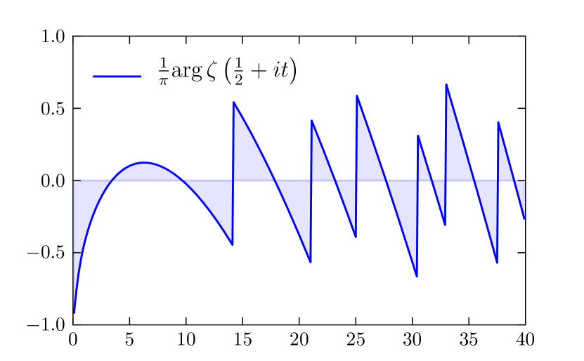
(a)

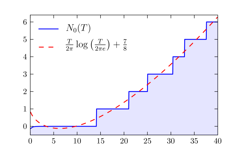
(b)

Figure 1: (a) A plot of $\tfrac{1}{\pi}\arg\zeta\left(\tfrac{1}{2}+it\right)$ as a function of $t$ showing its rapid oscillation. The jumps occur on a Riemann zero. (b) The function $N_{0}(T)$ in (14), which is indistinguishable from a manual counting of zeros. The dashed line is the smooth part without the $\arg\zeta$ term.

Remark 1.

The small shift by $\delta$ in equations (20) or (13) is essential since it smooths out $S(t)=\tfrac{1}{\pi}\arg\zeta\left(\tfrac{1}{2}+it\right)$, which is known to jump discontinuously at each Riemann zero. As is well known, $S(t)$ is a piecewise continuous function that rapidly oscillates around its average value, which is zero, with discontinuous jumps, as shown in Figure 1a. However, when $S(t)$ is added to the smooth part of $N(T)$ one obtains an accurate staircase function, which jumps by the multiplicity of the zero at the ordinate of each Riemann zero; see Figure 1b. Note that $N(T)$ is necessarily a monotonically increasing function since it is a counting formula.

One reason $\delta$ needs to be positive in (20) can be seen as follows. Near a simple zero $\rho_{n}$ we have $\zeta(s)\approx\left(s-\rho_{n}\right)\zeta^{\prime}\left(\rho_{n}\right)=\left(\delta+i\left(t-t_{n}\right)\right)\zeta^{\prime}\left(\rho_{n}\right)$. This gives $\arg\zeta(s)\sim\arctan\left((t-t_{n})/\delta\right)+c$, where $c$ is a constant. With $\delta>0$ as one passes through a zero from below, $S(t)$ increases by one, as it should based on its role in the counting formula $N(T)$. On the other hand, if $\delta<0$ then $S(t)$ would decrease by one instead, which cannot be the case.

Remark 2.

An important consequence of equation (20) is that, again, if it has a unique solution for every $n$, then all non-trivial zeros are simple. This essentially follows from the fact that they are in one-to-one correspondence with the zeros of the cosine function (11), which are simple. To see this, let us suppose there is a double zero at ordinate $t_{\bullet}$, i.e. $t_{n+1}=t_{n}=t_{\bullet}$. Then subtracting the equation (20) with $t_{n}$ from the corresponding equation with $t_{n+1}$, we obtain a contradiction, namely $0=\pi$. Therefore, for $n\neq m$ the equation (20) implies $t_{n}\neq t_{m}$.

Now if we actually assume that the zeros on the critical line are simple (which we have not), there is an easier way to see that the zeros correspond to $\cos\theta=0$. On the critical line $s=\tfrac{1}{2}+it$, the functional equation (2) implies $\chi(s)$ is real, thus for $t$ not the ordinate of a zero, $\sin\theta=0$ and $\cos\theta=\pm 1$. Thus $\cos\theta$ is a discontinuous function. Now let $t_{\bullet}$ be the ordinate of a simple zero. Then close to such a zero we define

$$c(t)\equiv\frac{\chi(\tfrac{1}{2}+it)}{|\chi(\tfrac{1}{2}+it)|}\sim\frac{t-t_{\bullet}}{|t-t_{\bullet}|}.$$ (23)

For $t>t_{\bullet}$ then $c(t)=1$, and for $t<t_{\bullet}$ then $c(t)=-1$. Thus $c(t)$ is discontinuous precisely at the zero. In the above polar representation, formally $c(t)=\cos\theta\left(\tfrac{1}{2},t\right)$. Therefore, by identifying zeros as the solutions to $\cos\theta=0$, we are simply defining the value of the function $c(t)$ at the discontinuity as $c(t_{\bullet})=0$.

Remark 3.

Let us introduce another function $\zeta(s)\to\widetilde{\zeta}(s)=f(s)\zeta(s)$ that also satisfies the functional equation (2), i.e. $\widetilde{\chi}(s)=\widetilde{\chi}(1-s)$, but has zeros off of the critical line due to the zeros of $f(s)$. In such a case the corresponding functional equation will hold if and only if $f(s)=f(1-s)$ for any $s$, and this is a trivial condition on $f(s)$ which could have been canceled in the first place. Moreover, if $f(s)$ and $\zeta(s)$ have different zeros, the analog of equation (8) has a factor $f(s)$, i.e. $\widetilde{\chi}(\rho+\delta)+\widetilde{\chi}(1-\rho-\delta)=f(\rho+\delta)\left[\chi(\rho+\delta)+\chi(1-\rho-\delta)\right]=0$, implying (8) again where $\chi(s)$ is the original (1). Therefore, the previous analysis eliminates $f(s)$ automatically and only finds the zeros of $\chi(s)$. The analysis is non-trivial precisely because $\zeta(s)$ satisfies the functional equation but $\zeta(s)\neq\zeta(1-s)$. Furthermore, it is a well-known theorem that the only function which satisfies the functional equation (2) and has the same characteristics of $\zeta(s)$, is $\zeta(s)$ itself. In other words, if $\widetilde{\zeta}(s)$ is required to have the same properties of $\zeta(s)$, then $\widetilde{\zeta}(s)=C\,\zeta(s)$ where $C$ is a constant (Titchmarsh, , pg. 31).

Remark 4.

Although equations (20) and (22) have an obvious resemblance, it is impossible to derive the former from the later, since the later is just a counting formula valid on the entire strip, and it is assumed that $T$ is not the ordinate of a zero. Moreover, such a derivation would require the assumption of the validity of the RH and the simplicity of the zeros, contrary to our approach, where we derived equations (20) and (13) directly on the critical line, without assuming the RH, nor the known counting formula $N(T)$. Despite our best efforts, we were not able to find equations (13) and (20) in the literature. Furthermore, the counting formulas (14) and (22) have never been proven to be valid on the critical line Edwards .

Remark 5.

One may object that our basic equation (20) involves $\zeta(s)$ itself and this is somehow circular. This is not a valid counter-argument. First of all, $\arg\zeta$ already appears in the counting function $N(T)$. Secondly, the equation (20) is a much more detailed equation than simply $\zeta(s)=0$, which has an infinite number of solutions, in contrast with (20) which for each $n$, as we have argued, has a unique solution corresponding to the $n$-th zero. Also, there are well known ways to calculate $\arg\zeta$, for example from an integral representation or a convergent series Borwein .

III Zeros of Dirichlet $L$-functions

III.1 Some properties of Dirichlet $L$-functions

We now consider the generalization of the previous results to Dirichlet $L$-functions. Let us first introduce the basic ingredients and definitions regarding this class of functions, which are all well known Apostol . Dirichlet $L$-series are defined as

$$L(s,\chi)=\sum_{n=1}^{\infty}\frac{\chi(n)}{n^{s}}$$ (24)

for $\Re(s)>1$, where the arithmetic function $\chi(n)$ is a Dirichlet character. They can all be analytically continued to the entire complex plane, except possibly for a simple pole at $s=1$ when $\chi$ is principal, and are then referred to as Dirichlet $L$-functions.

There are an infinite number of distinct Dirichlet characters which are primarily characterized by their modulus $k$, which determines their periodicity. They can be defined axiomatically, which leads to specific properties, some of which we now describe. Consider a Dirichlet character $\chi$ mod $k$, and let the symbol $(n,k)$ denote the greatest common divisor of the two integers $n$ and $k$. Then $\chi$ has the following properties:

1. $\chi(n+k)=\chi(n)$.

2. $\chi(1)=1$ and $\chi(0)=0$.

3. $\chi(n\,m)=\chi(n)\chi(m)$.

4. $\chi(n)=0$ if $(n,k)>1$ and $\chi(n)\neq 0$ if $(n,k)=1$.

5. If $(n,k)=1$ then $\chi(n)^{\varphi(k)}=1$, where $\varphi(k)$ is the Euler totient arithmetic function. This implies that $\chi(n)$ are roots of unity.

6. If $\chi$ is a Dirichlet character so is the complex conjugate $\overline{\chi}$.

For a given modulus $k$ there are $\varphi(k)$ distinct Dirichlet characters, which essentially follows from Property 5 above. They can thus be labeled as $\chi_{k,j}$ where $j=1,2,\dotsc,\varphi(k)$ denotes an arbitrary ordering. If $k=1$ we have the trivial character where $\chi(n)=1$ for every $n$, and (24) reduces to the Riemann $\zeta$-function. The principal character, usually denoted by $\chi_{1}$, is defined as $\chi_{1}(n)=1$ if $(n,k)=1$ and zero otherwise. In the above notation the principal character is always $\chi_{k,1}$.

Characters can be classified as primitive or non-primitive. Consider the Gauss sum

$$G(\chi)=\sum_{m=1}^{k}\chi(m)e^{2\pi im/k}.$$ (25)

If the character $\chi$ mod $k$ is primitive, then $|G(\chi)|^{2}=k$. This is no longer valid for a non-primitive character. Consider a non-primitive character $\widetilde{\chi}$ mod $\widetilde{k}$. Then it can be expressed in terms of a primitive character of smaller modulus as $\widetilde{\chi}(n)=\widetilde{\chi_{1}}(n)\chi(n)$, where $\widetilde{\chi_{1}}$ is the principal character mod $\widetilde{k}$ and $\chi$ is a primitive character mod $k<\widetilde{k}$, where $k$ is a divisor of $\widetilde{k}$. More precisely, $k$ must be the conductor of $\widetilde{\chi}$ (see Apostol for further details). In this case the two $L$-functions are related as $L(s,\widetilde{\chi})=L(s,\chi)\Pi_{p|\widetilde{k}}\left(1-\chi(p)/p^{s}\right)$. Thus $L(s,\widetilde{\chi})$ has the same zeros as $L(s,\chi)$. Therefore, it suffices to consider primitive characters, and we will henceforth do so.

We will need the functional equation satisfied by $L(s,\chi)$. Let $\chi$ be a primitive character. Define its order $a$ such that

$$a\equiv\begin{cases}1&\mbox{if $\chi(-1)=-1$ (odd)}\\ 0&\mbox{if $\chi(-1)=1$ (even)}\end{cases}.$$ (26)

Let us define the entire function

$$\Lambda(s,\chi)\equiv\left(\dfrac{k}{\pi}\right)^{\tfrac{s+a}{2}}\Gamma\left(\dfrac{s+a}{2}\right)L(s,\chi).$$ (27)

Then $\Lambda$ satisfies the following well-known functional equation, only valid for primitive characters Apostol :

$$\Lambda(s,\chi)=\dfrac{i^{-a}\,G(\chi)}{\sqrt{k}}\,\Lambda(1-s,\overline{\chi}).$$ (28)

III.2 Exact equation for the $n$-th zero

For a primitive character, since $|G(\chi)|=\sqrt{k}$, the factor on the right hand side of (28) is a phase. It is thus possible to obtain a more symmetric form through a new function defined as

$$\xi(s,\chi)\equiv\dfrac{i^{a/2}\,k^{1/4}}{\sqrt{G\left(\chi\right)}}\,\,\Lambda(s,\chi).$$ (29)

It then satisfies

$$\xi(s,\chi)=\overline{\xi}(1-s,\chi)\equiv\overline{\xi(1-\overline{s},\chi)}.$$ (30)

Above, the function $\overline{\xi}$ of $s$ is defined as the complex conjugation of all coefficients that define $\xi$, namely $\chi$ and the $i^{a/2}$ factor, evaluated at a non-conjugated $s$.

Note that $\overline{\Lambda(s,\chi)}=\Lambda(\overline{s},\overline{\chi})$. Using the known result $G\left(\overline{\chi}\right)=\chi(-1)\overline{G(\chi)}$ we then conclude that

$$\overline{\xi(s,\chi)}=\xi\left(\overline{s},\overline{\chi}\right).$$ (31)

This implies that if the character is real, when $\rho$ is a zero of $\xi$ so is $\overline{\rho}$, and one needs only to consider $\rho$ with positive imaginary part. On the other hand if $\chi\neq\overline{\chi}$, then the zeros with negative imaginary part are different than $\overline{\rho}$. For the trivial character where $k=1$ and $a=0$, implying $\chi(n)=1$ for any $n$, then $L(s,\chi)$ reduces to the Riemann $\zeta(s)$ and (30) yields the well-known functional equation (2).

Let $s=\sigma+it$. Then the function (29) can be written as $\xi(s,\chi)=Ae^{i\theta}$ where

$$A(\sigma,t,\chi) =\left(\dfrac{k}{\pi}\right)^{\tfrac{\sigma+a}{2}}\left|\Gamma\left(\dfrac{\sigma+a+it}{2}\right)\right|\left|L(\sigma+it,\chi)\right|,$$ (32)

$$\theta(\sigma,t,\chi) =\arg\Gamma\left(\dfrac{\sigma+a+it}{2}\right)-\dfrac{t}{2}\log\left(\dfrac{\pi}{k}\right)-\dfrac{1}{2}\arg G(\chi)$$ (33)

$$\qquad+\arg L(\sigma+it,\chi)+\dfrac{\pi a}{4}.$$

From (31) we have that $A(\sigma,t,\chi)=A(\sigma,-t,\overline{\chi})$ and $\theta(\sigma,t,\chi)=-\theta(\sigma,-t,\overline{\chi})$. Denoting $\overline{\xi}(1-s,\chi)=A^{\prime}e^{-i\theta^{\prime}}$ we then have $A^{\prime}(\sigma,t,\chi)=A(1-\sigma,t,\chi)$ and $\theta^{\prime}(\sigma,t,\chi)=\theta(1-\sigma,t,\chi)$. Taking the modulus of (30) we also have that $A(\sigma,t,\chi)=A^{\prime}(\sigma,t,\chi)$ for any $s$.

On the critical strip, the functions $L(s,\chi)$ and $\xi(s,\chi)$ have the same zeros. Thus on a zero we clearly have

$$\lim_{\delta\to 0^{+}}\left\{\xi(\rho+\delta,\chi)+\overline{\xi}(1-\rho-\delta,\chi)\right\}=0.$$ (34)

Let us define

$$B(\sigma,t,\chi)\equiv e^{i\theta(\sigma,t,\chi)}+e^{-i\theta^{\prime}(\sigma,t,\chi)}.$$ (35)

Since $A=A^{\prime}$ everywhere, from (34) we conclude that on a zero we have

$$\lim_{\delta\to 0^{+}}A(\sigma+\delta,t,\chi)B(\sigma+\delta,t,\chi)=0.$$ (36)

As before, let us consider the particular solution of $\lim_{\delta\to 0^{+}}B=0$ given by

$$\theta=\theta^{\prime},\qquad\lim_{\delta\to 0^{+}}\cos\theta=0.$$ (37)

Let us define the function

$$\begin{split}\vartheta_{k,a}(t)&\equiv\arg\Gamma\left(\dfrac{1}{4}+\dfrac{a}{2}+i\,\dfrac{t}{2}\right)-\dfrac{t}{2}\log\left(\dfrac{\pi}{k}\right)\\ &=\Im\left[\log\Gamma\left(\dfrac{1}{4}+\dfrac{a}{2}+i\,\dfrac{t}{2}\right)\right]-\dfrac{t}{2}\log\left(\dfrac{\pi}{k}\right).\end{split}$$ (38)

When $k=1$ and $a=0$, the function (38) is just the usual Riemann-Siegel $\vartheta$ function (19). Since the function $\log\Gamma$ has a complicated branch cut, one can use the following series representation in (38) Boros

$$\log\Gamma(s)=-\gamma s-\log s-\sum_{n=1}^{\infty}\left\{\log\left(1+\dfrac{s}{n}\right)-\dfrac{s}{n}\right\},$$ (39)

where $\gamma$ is the Euler-Mascheroni constant. Nevertheless, most numerical packages already have the $\log\Gamma$ function implemented.

On the critical line $\sigma=\tfrac{1}{2}$ the first equation in (37) is already satisfied. From the second equation we have $\lim_{\delta\to 0^{+}}\theta\left(\tfrac{1}{2}+\delta,t\right)=\left(n+\tfrac{1}{2}\right)\pi$, therefore

$$\vartheta_{k,a}(t_{n})+\lim_{\delta\to 0^{+}}\arg L\left(\tfrac{1}{2}+\delta+it_{n},\chi\right)-\dfrac{\arg G}{2}+\dfrac{\pi a}{4}=\left(n+\dfrac{1}{2}\right)\pi.$$ (40)

Analyzing the left hand side of (40) we can see that it has a minimum, thus we shift $n\to n-(n_{0}+1)$ for a given $n_{0}$, to label the zeros according to the convention that the first positive zero is labelled by $n=1$. Thus the upper half of the critical line will have the zeros labelled by $n=1,2,\dotsc$ corresponding to positive $t_{n}$, while the lower half will have the negative values $t_{n}$ labelled by $n=0,-1,\dotsc$. The integer $n_{0}$ depends on $k$, $a$ and $\chi$, and should be chosen according to each specific case. In the cases we analyze below $n_{0}=0$, whereas for the trivial character $n_{0}=1$. Henceforth we will omit the integer $n_{0}$ in the equations, since all cases analyzed in the following have $n_{0}=0$. Nevertheless, the reader should bear in mind that for other cases, it may be necessary to replace $n\to n-n_{0}$ in the following equations.

In summary, there are an infinite number of zeros on the critical line, i.e. in the form $\rho_{n}=\tfrac{1}{2}+it_{n}$, where for a given $n\in\mathbb{Z}$, the imaginary part $t_{n}$ is the solution of the equation

$$\vartheta_{k,a}(t_{n})+\lim_{\delta\to 0^{+}}\arg L\left(\tfrac{1}{2}+\delta+it_{n},\chi\right)-\dfrac{\arg G\left(\chi\right)}{2}=\left(n-\dfrac{1}{2}-\dfrac{a}{4}\right)\pi.$$ (41)

III.3 Asymptotic equation for the $n$-th zero

From Stirling’s formula we have the following asymptotic form for $t\to\pm\infty$:

$$\vartheta_{k,a}(t)=\mathrm{sgn}(t)\left[\dfrac{|t|}{2}\log\left(\dfrac{k|t|}{2\pi e}\right)+\dfrac{2a-1}{8}\pi+O(1/t)\right].$$ (42)

The first order approximation of (41), i.e. neglecting $O(1/t)$ terms, is therefore given by

$$\begin{split}\nu_{n}\dfrac{|t_{n}|}{2\pi}\log\left(\dfrac{k\,|t_{n}|}{2\pi e}\right)&+\dfrac{1}{\pi}\lim_{\delta\to 0^{+}}\arg L\left(\tfrac{1}{2}+\delta+i\nu_{n}|t_{n}|,\chi\right)\\ &-\dfrac{1}{2\pi}\arg G\left(\chi\right)=n+\dfrac{\nu_{n}-4-2a(1+\nu_{n})}{8},\end{split}$$ (43)

where $\nu_{n}=1$ if $n>0$ and $\nu_{n}=-1$ if $n\leq 0$. For $n>0$ we have $t_{n}=|t_{n}|$ and for $n\leq 0$ we have $t_{n}=-|t_{n}|$.

III.4 Counting formulas

Let us define $N^{+}_{0}(T,\chi)$ as the number of zeros on the critical line with $0<\Im(\rho)<T$ and $N^{-}_{0}(T,\chi)$ as the number of zeros with $-T<\Im(\rho)<0$. As explained before, $N^{+}_{0}(T,\chi)\neq N^{-}_{0}(T,\chi)$ if the characters are complex numbers, since the zeros are not symmetrically distributed between the upper and lower half of the critical line.

The counting formula $N^{+}_{0}(T,\chi)$ is obtained from equation (41) by replacing $t_{n}\to T$ and $n\to N^{+}_{0}+\tfrac{1}{2}$, therefore

$$N^{+}_{0}(T,\chi)=\dfrac{1}{\pi}\vartheta_{k,a}(T)+\dfrac{1}{\pi}\arg L\left(\tfrac{1}{2}+iT,\chi\right)-\dfrac{1}{2\pi}\arg G\left(\chi\right)+\dfrac{a}{4}.$$ (44)

The passage from (41) to (44) is justified under the assumptions already discussed in connection with (14) and (21), i.e. assuming that (41) has a unique solution for every $n$. As explained above for the Riemann $\zeta$ case, this is equivalent to assume the existence of the $\lim_{\delta\to 0^{+}}\arg L\left(\tfrac{1}{2}+\delta+it,\chi\right)$ for every $t$. Analogously, the counting formula on the lower half line is given by

$$N_{0}^{-}(T,\chi)=\dfrac{1}{\pi}\vartheta_{k,a}(T)-\dfrac{1}{\pi}\arg L\left(\tfrac{1}{2}-iT,\chi\right)+\dfrac{1}{2\pi}\arg G(\chi)-\dfrac{a}{4}.$$ (45)

Note that in (44) and (45) $T$ is positive. Both cases are plotted in Figure 2 for the character $\chi_{7,2}$ shown in (81). One can notice that they are precisely staircase functions, jumping by one at each zero. Note also that the functions are not symmetric about the origin.

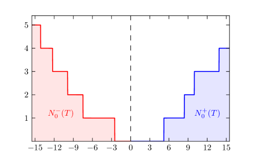
Figure 2: Exact counting formulae (44) and (45). Note that they are not symmetric with respect to the origin, since the $L$-zeros for complex $\chi$ are not complex conjugates. We used $\chi=\chi_{7,2}$ shown in (81).

From (42) we also have the first order approximation for $T\to\infty$,

$$N^{+}_{0}(T,\chi)=\dfrac{T}{2\pi}\log\left(\dfrac{k\,T}{2\pi e}\right)+\dfrac{1}{\pi}\arg L\left(\tfrac{1}{2}+iT,\chi\right)-\dfrac{\arg G}{2\pi}-\dfrac{1}{8}+\dfrac{a}{2}.$$ (46)

Analogously, for the lower half line we have

$$N^{-}_{0}(T,\chi)=\dfrac{T}{2\pi}\log\left(\dfrac{k\,T}{2\pi e}\right)-\dfrac{1}{\pi}\arg L\left(\tfrac{1}{2}-iT,\chi\right)+\dfrac{\arg G}{2\pi}-\dfrac{1}{8}.$$ (47)

As in (41) again we are omitting $n_{0}$ since in the cases below $n_{0}=0$, but for other cases one may need to include $\pm n_{0}$ on the right hand side of $N_{0}^{\pm}$, respectively.

It is known that the number of zeros on the entire critical strip up to height $T$, i.e. in the region $\{0<\sigma<1,\,0<t<T\}$, is given by Montgomery

$$N^{+}(T,\chi)=\dfrac{1}{\pi}\vartheta_{k,a}\left(T\right)+\dfrac{1}{\pi}\arg L\left(\tfrac{1}{2}+iT,\chi\right)-\dfrac{1}{\pi}\arg L\left(\tfrac{1}{2},\chi\right).$$ (48)

From Stirling’s approximation and noticing that $2a-1=-\chi(-1)$, then for $T\to\infty$ we obtain the asymptotic approximation Selberg1 ; Montgomery

$$\begin{split}N^{+}(T,\chi)&=\dfrac{T}{2\pi}\log\left(\dfrac{k\,T}{2\pi e}\right)+\dfrac{1}{\pi}\arg L\left(\tfrac{1}{2}+iT,\chi\right)\\ &-\dfrac{1}{\pi}\arg L\left(\tfrac{1}{2},\chi\right)-\dfrac{\chi(-1)}{8}+O(1/T).\end{split}$$ (49)

Both formulas (48) and (49) are exactly the same as (44) and (46), respectively. This can be seen as follows. From (30) we conclude that $\xi$ is real on the critical line. Thus $\arg\xi\left(\tfrac{1}{2}\right)=0=-\tfrac{1}{2}\arg G\left(\chi\right)+\arg L\left(\tfrac{1}{2},\chi\right)+\tfrac{\pi a}{4}$. Then, replacing $\arg G\left(\chi\right)$ in (41) we obtain

$$\vartheta_{k,a}\left(t_{n}\right)+\lim_{\delta\to 0^{+}}\arg L\left(\tfrac{1}{2}+\delta+it_{n},\chi\right)-\arg L\left(\tfrac{1}{2},\chi\right)=\left(n-\tfrac{1}{2}\right)\pi.$$ (50)

Replacing $t_{n}\to T$ and $n\to N_{0}^{+}+\tfrac{1}{2}$ in (50) we have precisely the expression (48), and also (49) for $T\to\infty$. Then we conclude that $N_{0}^{+}(T,\chi)=N^{+}(T,\chi)$ exactly. From (31) we see that negative zeros for character $\chi$ correspond to positive zeros for character $\overline{\chi}$. Thus for $-T<\Im(\rho)<0$ the counting on the critical strip also coincides with the counting on the critical line, since $N_{0}^{-}(T,\chi)=N_{0}^{+}(T,\overline{\chi})$ and $N^{-}(T,\chi)=N^{+}(T,\overline{\chi})$. Therefore, the number of zeros on the entire critical strip is the same as the number of zeros on the critical line obtained as solutions of (41), under the assumption that (41) has a unique solution for every $n$. This is equivalent to stating that $\lim_{\delta\to 0^{+}}\arg L\left(\tfrac{1}{2}+\delta+it,\chi\right)$ exists for every $t$. This will be further exemplified in Section VI.

IV Zeros of $L$-functions based on modular forms

Let us generalize the previous results to $L$-functions based on level one modular forms. We first recall some basic definitions and properties. The modular group can be represented by the set of $2\times 2$ integer matrices

$$SL_{2}\left(\mathbb{Z}\right)=\left\{A=\begin{pmatrix}[0.7]a&b\\ c&d\end{pmatrix}\,\bigg{|}\,\,a,b,c,d\in\mathbb{Z},\ \det A=1\right\},$$ (51)

provided each matrix $A$ is identified with $-A$, i.e. $\pm A$ are regarded as the same transformation. Thus for $\tau$ in the upper half complex plane, it transforms as $\tau\mapsto A\tau=\tfrac{a\tau+b}{c\tau+d}$ under the action of the modular group. A modular form $f$ of weight $k$ is a function that is analytic in the upper half complex plane which satisfies the functional relation Apostolmodular

$$f\left(\dfrac{a\tau+b}{c\tau+d}\right)=\left(c\tau+d\right)^{k}f(\tau).$$ (52)

If the above equation is satisfied for all of $SL_{2}\left(\mathbb{Z}\right)$, then $f$ is referred to as being of level one. It is possible to define higher level modular forms which satisfy the above equation for a subgroup of $SL_{2}\left(\mathbb{Z}\right)$. Since our results are easily generalized to the higher level case, henceforth we will only consider level one forms.

For the $SL_{2}\left(\mathbb{Z}\right)$ element $\begin{pmatrix}[0.6]1&1\\ 0&1\end{pmatrix}$, the above equation (52) implies the periodicity $f(\tau)=f(\tau+1)$, thus it has a Fourier series

$$f(\tau)=\sum_{n=0}^{\infty}a_{f}(n)\,q^{n},\qquad q\equiv e^{2\pi i\tau}.$$ (53)

If $a_{f}(0)=0$ then $f$ is called a cusp form.

From the Fourier coefficients, one can define the Dirichlet series

$$L_{f}\left(s\right)=\sum_{n=1}^{\infty}\dfrac{a_{f}\left(n\right)}{n^{s}}.$$ (54)

The functional equation for $L_{f}\left(s\right)$ relates it to $L_{f}\left(k-s\right)$, so that the critical line is $\Re(s)=\tfrac{k}{2}$, where $k\geq 4$ is an even integer. One can always shift the critical line to $\tfrac{1}{2}$ by replacing $a_{f}(n)\to a_{f}(n)/n^{(k-1)/2}$, however we will not do this here. Let us define

$$\Lambda_{f}(s)\equiv\left(2\pi\right)^{-s}\,\Gamma\left(s\right)\,L_{f}(s).$$ (55)

Then the functional equation is given by Apostolmodular

$$\Lambda_{f}(s)=(-1)^{k/2}\Lambda_{f}(k-s).$$ (56)

There are only two cases to consider since $\tfrac{k}{2}$ can be an even or an odd integer. As in (29) we can absorb the extra minus sign factor for the odd case. Thus we define $\xi_{f}(s)\equiv\Lambda_{f}(s)$ for $\tfrac{k}{2}$ even, and then $\xi_{f}(s)=\xi_{f}(k-s)$. For $\tfrac{k}{2}$ odd we define $\xi_{f}(s)\equiv e^{-i\pi/2}\Lambda_{f}(s)$ implying $\xi_{f}(s)=\overline{\xi_{f}}(k-s)$. Representing $\xi_{f}(s)=|\xi_{f}|\,e^{i\theta}$ where $s=\sigma+it$, we follow exactly the same steps as in the previous sections. From the particular solution (37) we conclude that there are infinite zeros on the critical line $\Re(\rho)=\tfrac{k}{2}$ determined by $\lim_{\delta\to 0^{+}}\theta\left(\tfrac{k}{2}+\delta,t\right)=\left(n-\tfrac{1}{2}\right)\pi$. Therefore, these zeros are given in the form $\rho_{n}=\tfrac{k}{2}+it_{n}$, where $t_{n}$ is the solution of the equation

$$\vartheta_{k}(t_{n})+\lim_{\delta\to 0^{+}}\arg L_{f}\left(\tfrac{k}{2}+\delta+it_{n}\right)=\left(n-\dfrac{1+(-1)^{k/2}}{4}\right)\pi$$ (57)

where $n=1,2,\dotsc$ and we have defined

$$\vartheta_{k}(t)\equiv\arg\Gamma\left(\tfrac{k}{2}+it\right)-t\log 2\pi.$$ (58)

This implies that the number of solutions of (57) with $0<t<T$ is given by

$$N_{0}\left(T\right)=\dfrac{1}{\pi}\vartheta_{k}(T)+\dfrac{1}{\pi}\arg L_{f}\left(\tfrac{k}{2}+iT\right)-\dfrac{1-(-1)^{k/2}}{4}.$$ (59)

In the limit of large $t_{n}$, neglecting terms of $O(1/t)$, the equation (57) becomes

$$t_{n}\log\left(\frac{t_{n}}{2\pi e}\right)+\lim_{\delta\to 0^{+}}\arg L_{f}\left(\tfrac{k}{2}+\delta+it_{n}\right)=\left(n-\dfrac{k+(-1)^{k/2}}{4}\right)\pi.$$ (60)

V Approximate zeros in terms of the Lambert $W$-function

V.1 Explicit formula

We now show that it is possible to obtain an approximate solution to the previous transcendental equations with an explicit formula. In this approximation, there is indeed a unique solution to the equation for every $n$. Let us introduce the Lambert $W$-function Corless , which is defined for any complex number $z$ through the equation

$$W(z)e^{W(z)}=z.$$ (61)

The multi-valued $W$-function cannot be expressed in terms of other known elementary functions. If we restrict attention to real-valued $W(x)$ there are two branches. The principal branch occurs when $W(x)\geq-1$ and is denoted by $W_{0}$, or simply $W$ for short, and its domain is $x\geq-e^{-1}$. The secondary branch, denoted by $W_{-1}$, satisfies $W_{-1}(x)\leq-1$ for $-e^{-1}\leq x<0$. Since we are interested only in positive real-valued solutions, we just need the principal branch where $W$ is single-valued.

Let us start with the zeros of the $\zeta$-function, described by equation (13). Consider its leading order approximation, or equivalently its average since $\langle\arg\zeta\left(\tfrac{1}{2}+iy\right)\rangle=0$. Then we have the transcendental equation

$$\dfrac{\widetilde{t}_{n}}{2\pi}\log\left(\dfrac{\widetilde{t}_{n}}{2\pi e}\right)=n-\dfrac{11}{8}.$$ (62)

Through the transformation $\widetilde{t}_{n}=2\pi\left(n-\tfrac{11}{8}\right)x_{n}^{-1}$, this equation can be written as $x_{n}e^{x_{n}}=e^{-1}\left(n-\tfrac{11}{8}\right)$. Comparing with (61) we thus we obtain

$$\widetilde{t}_{n}=\dfrac{2\pi\left(n-\tfrac{11}{8}\right)}{W\left[e^{-1}\left(n-\tfrac{11}{8}\right)\right]}$$ (63)

where $n=1,2,\dotsc$.

Although the inversion from (62) to (63) is rather simple, it is very convenient since it is indeed an explicit formula depending only on $n$, and $W$ is included in most numerical packages. It gives an approximate solution for the ordinates of the Riemann zeros in closed form. The values computed from (63) are much closer to the Riemann zeros than Gram points, and one does not have to deal with violations of Gram’s law; see Remark 8.

Analogously, for Dirichlet $L$-functions, after neglecting the $\arg L$ term, the equation (43) yields a transcendental equation which can be written as $x_{n}e^{x_{n}}=kA_{n}e^{-1}$ through the transformation $|t_{n}|=2\pi A_{n}x_{n}^{-1}$, where

$$A_{n}\left(\chi\right)=\nu_{n}\left(n+\dfrac{\arg G(\chi)}{2\pi}\right)+\dfrac{1-4\nu_{n}-2a\left(\nu_{n}+1\right)}{8}.$$ (64)

Thus the approximate solution is explicitly given by

$$\widetilde{t}_{n}=\dfrac{2\pi\nu_{n}A_{n}\left(\chi\right)}{W\left[k\,e^{-1}A_{n}\left(\chi\right)\right]}$$ (65)

where $n=0,\pm 1,\pm 2,\dotsc$. In the above formula $n=1,2,\dotsc$ correspond to positive $t_{n}$ solutions, while $n=0,-1,\dotsc$ correspond to negative $t_{n}$ solutions. Contrary to the $\zeta$-function, in general, the zeros are not conjugate related along the critical line.

In the same way, ignoring the small $\arg L_{f}$ term in (60), the approximate solution for the imaginary part of the zeros of $L$-functions based on level one modular forms is given by

$$\widetilde{t}_{n}=\dfrac{A_{n}\pi}{W\left[(2e)^{-1}A_{n}\right]},\qquad A_{n}=n-\dfrac{k+(-1)^{k/2}}{4},\qquad n=1,2,\dotsc.$$ (66)

V.2 Further remarks

Let us focus on the approximation (63) regarding zeros of the $\zeta$-function. Obviously the same arguments apply to the zeros of the other classes of functions based on formulas (65) and (66).

Remark 6.

The estimates given by (63) can be calculated for arbitrarily large $n$, since $W$ is a standard elementary function. Of course the $\widetilde{t}_{n}$ are not as accurate as the solutions $t_{n}$ including the $\arg\zeta$ term, as we will see in Section VII. Nevertheless, it is indeed a good estimate, especially if one considers very high zeros where traditional methods have not previously estimated such high values. For instance, formula (63) can easily estimate the zeros shown in Table 1 (Appendix B.1), and much higher if desirable. The numbers in this table are accurate approximations to the $n$-th zero to the number of digits shown, which is approximately the number of digits in the integer part. For instance, the approximation to the $10^{100}$ zero is correct to $100$ digits. With Mathematica we easily calculated the first million digits of the $10^{10^{6}}$ zero.

Remark 7.

Using the asymptotic behaviour $W(x)\approx\log x$ for large $x$, the $n$-th zero is approximately given by $\widetilde{t}_{n}\approx 2\pi n/\log n$, as already known Titchmarsh . The distance between consecutive ordinates is then approximately equal to $\widetilde{t}_{n+1}-\widetilde{t}_{n}\approx 2\pi/\log n$, which tends to zero when $n\to\infty$.

Remark 8.

The solutions (63) are reminiscent of the so-called Gram points $g_{n}$, which are solutions to $\vartheta(g_{n})=n\pi$ where $\vartheta$ is given by (19). Gram’s law is the tendency for Riemann zeros to lie between consecutive Gram points, but it is known to fail for about $\tfrac{1}{4}$ of all Gram intervals. Our $\widetilde{t}_{n}$ are intrinsically different from Gram points. It is an approximate solution for the ordinate of the zero itself. In particular, the Gram point $g_{0}=17.8455$ is the closest to the first Riemann zero, whereas $\widetilde{t}_{1}=14.52$ is already much closer to the true zero which is $t_{1}\approx 14.1347$. The traditional method to compute the zeros is based on the Riemann-Siegel formula $\zeta\left(\tfrac{1}{2}+it\right)=Z(t)\left[\cos\vartheta(t)-i\sin\vartheta(t)\right]$, and the empirical observation that the real part of this equation is almost always positive, except when Gram’s law fails, and $Z(t)$ has the opposite sign of $\sin\vartheta$. Since $Z(t)$ and $\zeta\left(\tfrac{1}{2}+it\right)$ have the same zeros, one looks for the zeros of $Z(t)$ between two Gram points, as long as Gram’s law holds $(-1)^{n}Z\left(g_{n}\right)>0$. To verify the RH numerically, the counting formula (22) must also be used to assure that the number of zeros on the critical line coincide with the number of zeros on the strip. The detailed procedure is throughly explained in Edwards ; Titchmarsh . Based on this method, amazingly accurate solutions and high zeros on the critical line were computed Gourdon ; Odlyzko ; OdlyzkoSchonhage ; Odlyzko2 . Nevertheless, our proposal is fundamentally different. We claim that (20) is the equation that determines the Riemann zeros on the critical line. Then, one just needs to find its solution for a given $n$. We will compute the Riemann zeros in this way in the next section, just by solving the equation (20) numerically, starting from the approximation given by the explicit formula (63), without using Gram points nor the Riemann-Siegel $Z$ function. Let us emphasize that our goal is not to provide a more efficient algorithm to compute the zeros OdlyzkoSchonhage , although the method described here may very well be, but to justify the validity of equation (20).

VI A counterexample: the Davenport-Heilbronn function

In this section we consider a function that is known to violate the RH, and this serves to sharpen our understanding of our previous analysis. In this example, one can clearly see how the corresponding transcendental equation does not have a unique solution for every $n$.

The Davenport-Heilbronn function is defined by

$$\mathcal{D}(s)\equiv\dfrac{(1-i\kappa)}{2}L\left(s,\chi_{5,2}\right)+\dfrac{(1+i\kappa)}{2}L\left(s,\overline{\chi}_{5,2}\right)$$ (67)

with

$$\kappa=\dfrac{\sqrt{10-2\sqrt{5}}-2}{\sqrt{5}-1}.$$ (68)

Above the Dirichlet character is the following:

$$n$$

(69)

where $\chi_{5,2}(-1)=-1$ thus $a=1$. The function (67) satisfies the functional equation

$$\xi(s)=\xi(1-s),\qquad\xi(s)\equiv\left(\dfrac{\pi}{5}\right)^{-s/2}\,\Gamma\left(\dfrac{1+s}{2}\right)\mathcal{D}(s).$$ (70)

The function (67) has almost all the same properties of $\zeta$, such as a functional equation, except that it has no Euler Product Formula. It is well known that it has zeros in the region $\Re\left(s\right)>1$, which is essentially a consequence that it has no Euler product. It also has zeros in the critical strip $0\leq\Re(s)\leq 1$, where infinitely many of them lie on the critical line $\Re(s)=\tfrac{1}{2}$, however, it also has zeros off of the critical line, thus violating the RH. For a detailed study of this function and numerical computation of its zeros see BombieriGosh .

Repeating the analysis of the previous sections for zeros on the critical line, we obtain the following transcendental equation:

$$\dfrac{1}{\pi}\vartheta_{5,1}(t_{n})+\dfrac{1}{\pi}\lim_{\delta\to 0^{+}}\arg\mathcal{D}\left(\tfrac{1}{2}+\delta+it_{n}\right)+\dfrac{1}{2}=n$$ (71)

where $\vartheta_{5,1}$ is defined in (38). The approximate solution is explicitly given by

$$\widetilde{t}_{n}=\dfrac{2\pi\left(n-\tfrac{5}{8}\right)}{W\left[5e^{-1}(n-\tfrac{5}{8})\right]}$$ (72)

for $n=1,2,\dotsc$. From (71) and (72) it is possible to compute zeros on the critical line. Moreover, zeros off of the critical line satisfy the general solution (10) Lectures . This shows that $B=0$, with $B$ defined in (35), captures all the zeros.

Since (71) only captures zeros at $\sigma=\tfrac{1}{2}$, what happens if there are zeros off of the critical line? Consider a simple zero denoted by $\rho_{\bullet}=\sigma_{\bullet}+it_{\bullet}$ where $0<\sigma_{\bullet}<1$ and $\sigma_{\bullet}\neq\tfrac{1}{2}$. Due to the functional equation (70) there is also a zero at $1-\overline{\rho}_{\bullet}=1-\sigma_{\bullet}+it_{\bullet}$. Let

$$S_{\mathcal{D}}(t)=\dfrac{1}{\pi}\lim_{\delta\to 0^{+}}\arg\mathcal{D}\left(\tfrac{1}{2}+\delta+it\right).$$ (73)

From its role in the counting formula over the entire critical strip, one knows that when $t$ varies across $t_{\bullet}$ then $S_{\mathcal{D}}(t)$ must jump by two, i.e. we must have $\Delta S_{\mathcal{D}}(t_{\bullet})\equiv S_{\mathcal{D}}(t_{\bullet}+\epsilon)-S_{\mathcal{D}}(t_{\bullet}-\epsilon)=2$. This implies that $S_{\mathcal{D}}(t)$ changes branch around $t_{\bullet}$ in such a way that it cannot be smoothed out by the $\delta\to 0^{+}$ limit. In other words, the limit (73) does not exist close to $t_{\bullet}$. Therefore, (71) will not have a solution around $t_{\bullet}$ for a given $n$. If instead of a simple zero we have a zero with multiplicity $m\geq 2$, then $\Delta S_{\mathcal{D}}(t_{\bullet})=2m$, changing branch even more drastically. The same situation also happens if there are zeros with multiplicity $m\geq 2$ on the critical line, where we would have $\Delta S_{\mathcal{D}}=m$.

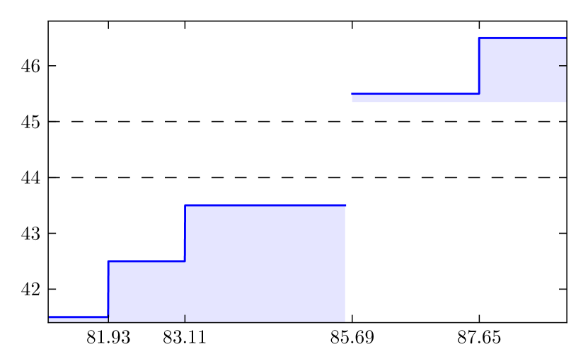
(a)

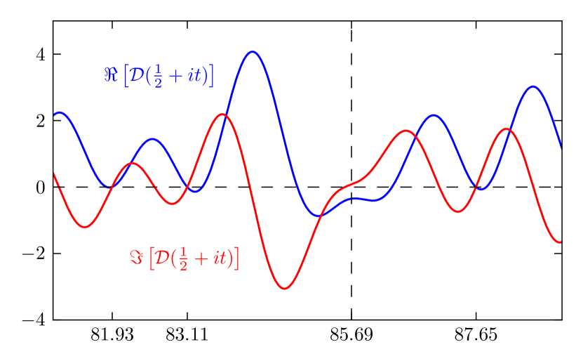
(b)

Figure 3: (a) Left hand side of (71) against $t$. Note the discontinuity at the point $t_{\bullet}\approx 85.6993$ corresponding to $n=44$ and $n=45$, where (71) has no solution. (b) We plot $\Re\left[\mathcal{D}(1/2+it)\right]$ (blue line) and $\Im\left[\mathcal{D}(1/2+it)\right]$ (red line) against $t$. Observe that $\Re\left[\mathcal{D}(1/2+it)\right]<0$ when $\Im\left[\mathcal{D}(1/2+it)\right]\to 0$, for $t\to t_{\bullet}$, signaling the change of branch of $\arg\mathcal{D}(1/2+it)$.

In the case of the function (67), the first zero off of the critical line occurs at $\sigma_{\bullet}\approx 0.8085$ and $t_{\bullet}\approx 85.6993$. In Figure 3a we plot the left hand side of (71) against $t$, and one can clearly see the above mentioned situation, namely that (71) is not defined at $t_{\bullet}$ and there is no solution for $n=44$ and $n=45$. The change of branch close to $t_{\bullet}$ can be seen from Figure 3b. Therefore, denoting $N_{0}(T)$ the number of solutions of (71) up to height $T$, we clearly have $N_{0}(T)<N(T)$, where $N(T)$ is the number of zeros in the entire critical strip. For a more detailed illustration of these facts we refer the reader to Lectures .

For simple zeros on the critical line the limit (73) exists, but for zeros off of the critical line, it does not, since $S_{\mathcal{D}}(t)$ has to jump at least by two and the change of branch does not allow us to smooth the function.

VII Numerical analysis: $\zeta$-function

VII.1 The importance of $\arg\zeta$

Instead of solving the exact equation (20) we will initially consider its first order approximation, which is equation (13). As we will see, this approximation already yields surprisingly accurate values for the Riemann zeros.

Let us first consider how the approximate solution given by (63) is modified by the presence of the $\arg\zeta$ term in (13). Numerically, we compute $\arg\zeta$ taking its principal value. The fact that we get very accurate zeros up to the billionth zero implies that up to this $t$, $\arg\zeta$ near a zero is always on the principal branch. As already discussed in Remark 1, the function $\arg\zeta\left(\tfrac{1}{2}+it\right)$ oscillates around its average, which is zero, as shown in Figure 1a. At a Riemann zero it can be defined by the limit (6) which is generally not zero. The $\arg\zeta$ term plays an important role and indeed improves the estimate of the $n$-th zero. This can be seen in Figure 4 where we compare the estimate given by (63) with the numerical solutions of (13).

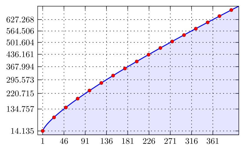
(a)

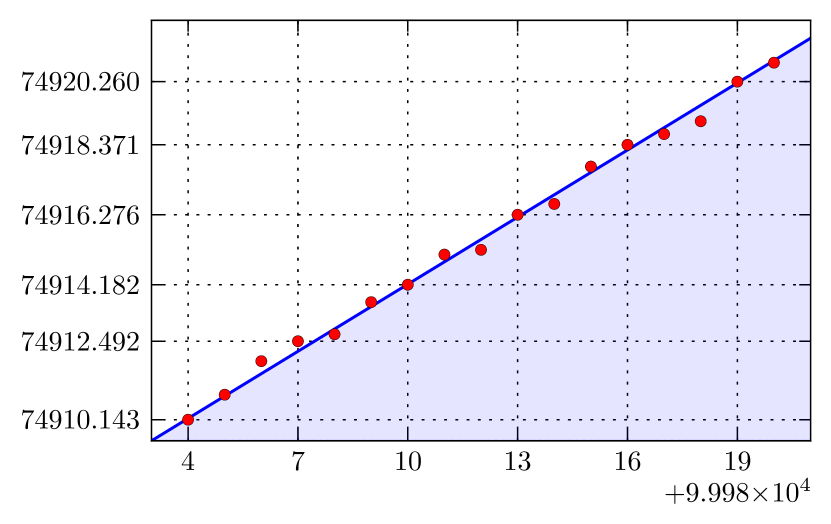
(b)

Figure 4: Comparison of the prediction of (63) (blue line) and (13) (red dots). We are plotting $t_{n}$ against $n$. (a) $n\in[1,\dotsc,400]$. Note how the solutions are close at first sight. (b) If we focus on a small range we can see how the solutions of (13) oscillate around the line (63) due to the fluctuating term $\arg\zeta$. Here $n\in[99984,\dotsc,10^{5}]$.

We can apply a root finder method in an appropriate interval, centered around the approximate solution $\widetilde{t}_{n}$ given by formula (63). Some of the solutions obtained in this way are presented in Table 2 (Appendix B.1) and are accurate up to the number of decimal places shown. We used only Mathematica or some very simple algorithms to perform these numerical computations, taken from standard open source numerical libraries.

Although the equation (13) was derived for large $n$, it is surprisingly accurate even for the lower zeros, as shown in Table 3 (Appendix B.1). It is actually easier to solve for low zeros since $\arg\zeta$ is better behaved. These numbers are correct up to the number of digits shown, and the precision was improved simply by decreasing the error tolerance.

VII.2 GUE statistics

The link between the Riemann zeros and random matrix theory started with the pair correlation of zeros, proposed by Montgomery Montgomery , and the observation of Dyson Dyson that it is the same as the 2-point correlation function predicted by the Gaussian Unitary Ensemble (GUE) for large random matrices.

The main purpose of this section is to test whether our approximation (13) to the zeros is accurate enough to reveal this statistics. Whereas formula (63) is a valid estimate, it is not sufficiently accurate to reproduce the GUE statistics, since it does not have the oscillatory $\arg\zeta$ term. On the other hand, the solutions to equation (13) are accurate enough, which again indicates the importance of $\arg\zeta$.

Montgomery’s pair correlation conjecture can be stated as follows:

$$\dfrac{1}{N(T)}\sideset{}{{}^{\prime}}{\sum}_{\begin{subarray}{c}0\leq t,t^{\prime}\leq T\\[2.79996pt] \alpha<d(t,t^{\prime})\leq\beta\end{subarray}}1\,\sim\,\int_{\alpha}^{\beta}du\left(1-\dfrac{\sin^{2}\left(\pi u\right)}{\pi^{2}u^{2}}\right),$$ (74)

where $d(t,t^{\prime})=\tfrac{1}{2\pi}\log\left(\tfrac{T}{2\pi}\right)\left(t-t^{\prime}\right)$, $0<\alpha<\beta$, $N(T)\sim\tfrac{T}{2\pi}\log\left(\tfrac{T}{2\pi}\right)$ according to (15), and the statement is valid in the limit $T\to\infty$. The right hand side of (74) is the 2-point GUE correlation function. The average spacing between consecutive zeros is given by $\tfrac{T}{N}\sim 2\pi/\log\left(\tfrac{T}{2\pi}\right)\to 0$ as $T\to\infty$. This can also be seen from (63) for very large $n$, i.e. $t_{n+1}-t_{n}\to 0$ as $n\to\infty$. Thus the distance $d(t,t^{\prime})$ between zeros on the left hand side of (74) is a normalized distance.

While (74) can be applied if we start from the first zero on the critical line, it is unable to provide a test if we are centered around a given high zero on the line. To deal with such a situation, Odlyzko Odlyzko2 proposed a stronger version of Montgomery’s conjecture by taking into account the large density of zeros higher on the line. This is done by replacing the normalized distance in (74) by a sum of normalized distances over consecutive zeros in the form

$$d_{n}\equiv\dfrac{1}{2\pi}\log\left(\dfrac{t_{n}}{2\pi}\right)\left(t_{n+1}-t_{n}\right).$$ (75)

Thus (74) is replaced by

$$\dfrac{1}{\left(N-M\right)\left(\beta-\alpha\right)}\sideset{}{{}^{\prime}}{\sum}_{\begin{subarray}{c}M\leq m,n\leq N\\[2.79996pt] \alpha<\sum_{k=1}^{n}d_{m+k}\leq\beta\end{subarray}}1\,=\,\dfrac{1}{\beta-\alpha}\int_{\alpha}^{\beta}du\left(1-\dfrac{\sin^{2}\left(\pi u\right)}{\pi^{2}u^{2}}\right),$$ (76)

where $M$ is the label of a given zero on the line and $N>M$. In this sum it is also assumed that $n>m$, and we included the correct normalization on both sides. The conjecture (76) is already well supported by extensive numerical analysis Odlyzko2 ; Gourdon .

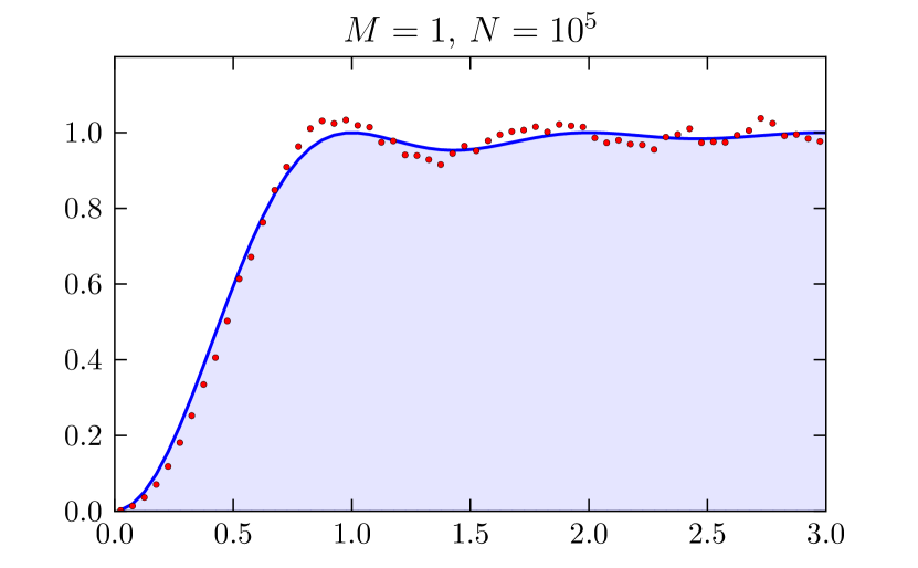
(a)

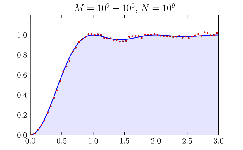
(b)

Figure 5: The solid line represents the right hand side of (76) and the dots represent its left hand side, computed from equation (13). The parameters are $\beta=\alpha+0.05$, $\alpha=(0,\,0.05,\,\dotsc,\,3)$ and the $x$-axis is given by $x=\tfrac{1}{2}\left(\alpha+\beta\right)$. (a) We use the first $10^{5}$ zeros. (b) The same parameters but using zeros in the middle of the critical line; $M=10^{9}-10^{5}$ and $N=10^{9}$.

Odlyzko’s conjecture (76) is a very strong constraint on the statistics of the zeros. Thus we submit the numerical solutions of equation (13) to this test. In Figure 5a we can see the result for $M=1$ and $N=10^{5}$, with $\alpha$ ranging from $0\dotsc 3$ in steps of $\epsilon=0.05$, and $\beta=\alpha+\epsilon$ for each value of $\alpha$, i.e. $\alpha=(0.00,\,0.05,\,0.10,\dotsc,\,3.00)$ and $\beta=(0.05,\,0.10,\,\dotsc,\,3.05)$. We compute the left hand side of (76) for each pair $(\alpha,\beta)$ and plot the result against $x=\tfrac{1}{2}\left(\alpha+\beta\right)$. In Figure 5b we do the same thing but with $M=10^{9}-10^{5}$ and $N=10^{9}$. Clearly, the numerical solutions of (13) reproduce the GUE statistics. In fact, Figure 5a is identical to the one in Odlyzko2 . The last zeros in these ranges are shown in Table 4 (Appendix B.1).

VII.3 Prime number counting function

In this section we explore whether our approximations to the Riemann zeros are accurate enough to reconstruct the prime number counting function. As usual, let $\pi(x)$ denote the number of primes less than $x$. Riemann obtained an explicit expression for $\pi(x)$ in terms of the non-trivial zeros of $\zeta(s)$. There are simpler but equivalent versions of the main result, based on the function $\psi(x)$ below. However, let us present the main formula for $\pi(x)$ itself since it is historically more important.

The function $\pi(x)$ is related to another number-theoretic function $J(x)$, defined as

$$J(x)=\sum_{2\leq n\leq x}\frac{\Lambda(n)}{\log n}$$ (77)

where $\Lambda(n)$, the von Mangoldt function, is defined as $\Lambda(n)=\log p$ if $n=p^{m}$ for some prime $p$ and an integer $m\geq 1$, and $\Lambda(n)=0$ otherwise. The two functions $\pi(x)$ and $J(x)$ are related by Möbius inversion:

$$\pi(x)=\sum_{n\geq 1}\frac{\mu(n)}{n}J(x^{1/n}).$$ (78)

Here $\mu(n)$ is the Möbius function defined as follows. $\mu(n)=0$ if $n$ has one or more repeated prime factors, $\mu(n)=1$ if $n=1$ and $\mu(n)=(-1)^{k}$ if $n$ is a product of $k$ distinct primes. The above expression is actually a finite sum, since for large enough $n$, $x^{1/n}<2$ and $J=0$.

The main result of Riemann is a formula for $J(x)$, expressed as an infinite sum over zeros $\rho$ of the $\zeta(s)$ function:

$$J(x)={\rm Li}(x)-\sum_{\rho}{\rm Li}\left(x^{\rho}\right)+\int_{x}^{\infty}\dfrac{dt}{\log t}~{}\dfrac{1}{t\left(t^{2}-1\right)}-\log 2,$$ (79)

where ${\rm Li}(x)=\int_{0}^{x}dt/\log t$ is the log-integral function. The above sum is real because the $\rho$’s come in conjugate pairs. If there are no zeros on the line $\Re(z)=1$, then the dominant term is the first one in the above equation, $J(x)\approx{\rm Li}(x)$, and this was used to prove the prime number theorem by Hadamard and de la Vallée Poussin.

The function $\psi(x)$ has the simpler form

$$\psi(x)=\sum_{n\leq x}\Lambda(n)=x-\sum_{\rho}\dfrac{x^{\rho}}{\rho}-\log(2\pi)-\dfrac{1}{2}\log\left(1-\dfrac{1}{x^{2}}\right).$$ (80)

In this formulation the prime number theorem is equivalent to $\psi(x)\approx x$.

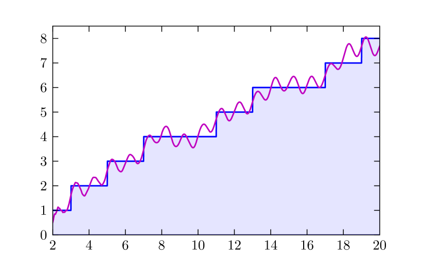
(a)

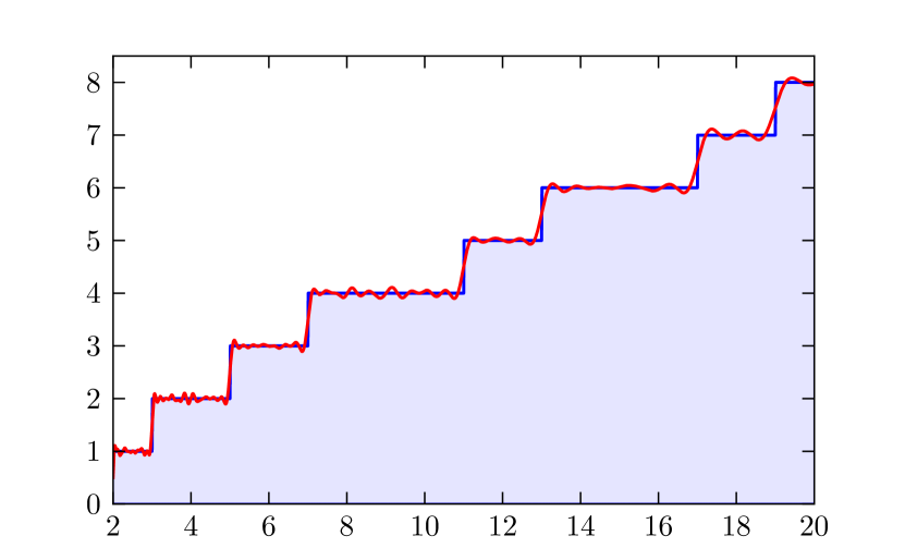
(b)

Figure 6: The prime number counting function $\pi(x)$ with the first $50$ Riemann zeros. (a) Zeros approximated by the formula (63). (b) Zeros obtained from numerical solutions to the equation (13).

In Figure 6a we plot $\pi(x)$ from equations (78) and (79), computed with the first $50$ zeros in the approximation $\rho_{n}=\tfrac{1}{2}+i\widetilde{t}_{n}$ given by (63). Figure 6b shows the same plot with zeros obtained from the numerical solutions of equation (13). Although with the approximation $\widetilde{t}_{n}$ the curve is trying to follow the steps in $\pi(x)$, once again, one clearly sees the importance of the $\arg\zeta$ term.

VII.4 Solutions to the exact equation

In the previous sections we have computed numerical solutions of (13) showing that, actually, this first order approximation to (20) is very good and already captures some interesting properties of the Riemann zeros, such as the GUE statistics and the ability to reproduce $\pi(x)$. Nevertheless, by simply solving (20) it is possible to obtain values for the zeros as accurately as desirable. The numerical procedure is performed as follows:

1. We apply a root finder method on (20) looking for the solution in a region centered around the number $\widetilde{t}_{n}$ provided by (63), with a not so small $\delta$, for instance $\delta\sim 10^{-5}$.

2. We solve (20) again but now centered around the solution obtained in step 1 above, and we decrease $\delta$, for instance $\delta\sim 10^{-8}$.

3. We repeat the procedure in step 2 above, decreasing $\delta$ again.

4. Through successive iterations, and decreasing $\delta$ each time, it is possible to obtain solutions as accurate as desirable. In carrying this out, it is important to not allow $\delta$ to be exactly zero.

An actual implementation of the above procedure in Mathematica is shown in Appendix A, which we have included mainly to show its simplicity. The first few zeros computed in this way are shown in Table 5 (Appendix B.1). Through successive iterations it is possible achieve even much higher accuracy than shown in Table 5.

It is known that the first zero where Gram’s law fails is for $n=126$. Applying the same method, like for any other $n$, the solution of (20) starting with the approximation (63) does not present any difficulty. We easily found the following number:

$$t_{126}=279.229250927745189228409880451955359283492637405561293594727$$

Just to illustrate, and to convince the reader, how the solutions of (20) can be made arbitrarily precise, we compute the zero $n=1000$ accurate up to $500$ decimal places, also using the same simple approach:

$$t_{1000}=1419. 42248094599568646598903807991681923210060106416601630$$

$$46908146846086764175930104179113432911792099874809842$$

$$32260560118741397447952650637067250834288983151845447$$

$$68825259311594423942519548468770816394625633238145779$$

$$15284185593431511879329057764279980127360524094461173$$

$$37041818962494747459675690479839876840142804973590017$$

$$35474131911629348658946395454231320810569901980719391$$

$$75430299848814901931936718231264204272763589114878483$$

$$29996467356160858436515425171824179566414953524432921$$

$$93649483857772253460088$$

Furthermore, one can substitute known precise Riemann zeros into (20) and can check that the equation is identically satisfied. These results corroborate that (20) is an exact equation for the Riemann zeros.

VIII Numerical analysis: $L$-functions

We perform exactly the same numerical procedure as described in the previous Section VII.4, but now with equation (41) and (65) for Dirichlet $L$-functions, or with (57) and (66) for $L$-functions based on level one modular forms.

VIII.1 Dirichlet $L$-functions

We will illustrate our formulas with the primitive characters $\chi_{7,2}$ and $\chi_{7,3}$ since they possess the full generality of $a=0$ and $a=1$ and complex components. There are actually $\varphi(7)=6$ distinct characters mod $7$.

Example $\chi_{7,2}$. Consider $k=7$ and $j=2$, i.e. we are computing the Dirichlet character $\chi_{7,2}(n)$. For this case $a=1$. Then we have the following components:

$$n$$

(81)

The first few zeros, positive and negative, obtained by solving (41) are shown in Table 6 in Appendix B.2. The solutions shown are easily obtained with $50$ decimal places of accuracy.

Example $\chi_{7,3}$. Consider $k=7$ and $j=3$, such that $a=0$. In this case the components of $\chi_{7,3}(n)$ are the following:

$$n$$

(82)

The first few solutions of (41) are shown in Table 7 in Appendix B.2 and are accurate up to $50$ decimal places. As previously stated, the solutions to equation (41) can be calculated to any desired level of accuracy. For instance, we can easily compute the following number for $n=1000$, accurate to $100$ decimal places:

$$t_{1000}=1037. 56371706920654296560046127698168717112749601359549$$

$$01734503731679747841764715443496546207885576444206$$

We also have been able to solve the equation for high zeros to high accuracy, up to the millionth zero, some of which are listed in Table 8 in Appendix B.2, and were previously unknown.

VIII.2 Modular $L$-function based on Ramanujan $\tau$

Here we will consider an example of a modular form of weight $k=12$. The simplest example is based on the Dedekind $\eta$-function

$$\eta(\tau)=q^{1/24}\,\prod_{n=1}^{\infty}(1-q^{n}),\qquad q=e^{2\pi i\tau}.$$ (83)

Up to a simple factor, $\eta$ is the inverse of the chiral partition function of the free boson conformal field theory CFT , where $\tau$ is the modular parameter of the torus. The modular discriminant

$$\Delta(\tau)=\eta(\tau)^{24}=\sum_{n=1}^{\infty}\,\tau(n)\,q^{n}$$ (84)

is a weight $k=12$ modular form. It is closely related to the inverse of the partition function of the bosonic string in $26$ dimensions, where $24$ is the number of light-cone degrees of freedom in $26$ spacetime dimensions String . The Fourier coefficients $\tau(n)$ correspond to the Ramanujan $\tau$-function, and the first few are

$$n$$

(85)

We then define the Dirichlet series

$$L_{\Delta}(s)=\sum_{n=1}^{\infty}\,\frac{\tau(n)}{n^{s}}.$$ (86)

Applying (57) the zeros are $\rho_{n}=6+it_{n}$, where $t_{n}$ satisfies the equation

$$\vartheta_{12}(t_{n})+\lim_{\delta\to 0^{+}}\arg L_{\Delta}(6+\delta+it_{n})=\left(n-\tfrac{1}{2}\right)\pi.$$ (87)

The counting formula (59) and its asymptotic approximation are

$$N_{0}(T) =\dfrac{1}{\pi}\vartheta_{12}(T)+\dfrac{1}{\pi}\arg L_{\Delta}(6+iT)$$ (88)

$$\simeq\dfrac{T}{\pi}\log\left(\dfrac{T}{2\pi e}\right)+\dfrac{1}{\pi}\arg L_{\Delta}(6+iT)+\dfrac{11}{4}.$$ (89)

A plot of (88) is shown in Figure 7, and we can see that it is a perfect staircase function. The approximate solution (66) now has the form

$$\widetilde{t}_{n}=\dfrac{\left(n-\tfrac{13}{4}\right)\pi}{W\left[(2e)^{-1}\left(n-\tfrac{13}{4}\right)\right]}\qquad\mbox{for $n=2,3,\dotsc$}.$$ (90)

Note that the above equation is valid for $n>1$ since $W(x)$ is not defined for $x<-1/e$.

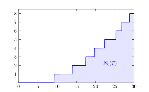
Figure 7: Exact counting formula (88) based on the Ramanujan $\tau$-function.

We follow exactly the same numerical procedure, previously discussed in Section VII.4 and implemented in Appendix A, to solve the equation (87) starting with the approximation provided by (90). Some of these solutions are shown in Table 9 in Appendix B.3 and are accurate to $50$ decimal places.

IX Concluding remarks

In this paper we considered non-trivial zeros of the Riemann $\zeta$-function, Dirichlet $L$-functions and $L$-functions based on level one modular forms. The same approach was applied to all these classes of functions, showing that there are an infinite number of zeros on the critical line in one-to-one correspondence with the zeros of the cosine function (11), leading to a transcendental equation satisfied by the ordinate of the $n$-th zero. More specifically, for the Riemann $\zeta$-function these zeros are solutions to (20), for Dirichlet $L$-functions we have (41), and for $L$-functions based on level one modular forms the ordinates of the zeros must satisfy (57). It is important to stress that these equations were derived on the critical line, without assuming the RH.

The implication of our work for the GRH can be summarized as follows. If the corresponding transcendental equation has a unique solution for every $n$, the validity of the GRH would follow. The explanation is very simple. Suppose the transcendental equation indeed has a unique solution for every $n$. Then the zeros obtained from its solutions on the critical line can be counted, since they are enumerated by the integer $n$, yielding the counting function $N_{0}(T)$. The number of solutions saturate the counting formula over the entire critical strip, namely $N_{0}(T)=N(T)$, where $N(T)$ counts zeros on the entire critical strip and has been known for a long time. Thus the equation captures all the non-trivial zeros.

As previously discussed, and explicitly illustrated in Section VI, the existence of solutions depends on whether the $\delta\to 0^{+}$ limit of the argument of the corresponding $L$-function is well-defined for every ordinate $t$. The validity of this limit was our only assumption throughout the paper. We also argued that if there is indeed a unique solution of the transcendental equation for every $n$, then all non-trivial zeros are simple. If there are zeros off of the critical line, or zeros with multiplicity $m\geq 2$ on the critical line, the equation will fail to capture all the zeros on the critical strip and then $N_{0}(T)<N(T)$. Does this means that the GRH is false if the transcendental equation does not always have a unique solution? Not necessarily, since all the zeros can still be on the critical line but not all of them are simple. This suggests that the GRH and the simplicity of all non-trivial zeros is equivalent to the statement that the transcendental equation has a unique solution for every $n$. We have not proven that there is a unique solution to the transcendental equation. An attempt to justify more carefully this $\delta\to 0^{+}$ limit is in our preliminary work EulerProd , where we claim that the Euler Product Formula is still valid in the region $\tfrac{1}{2}<\Re(s)\leq 1$ in a statistical manner.

We also showed that it is possible to obtain an explicit formula as an approximation for the ordinates of the zeros in terms of the Lambert $W$-function; equation (63) for the $\zeta$-function, (65) for Dirichlet $L$-functions and (66) for $L$-functions based on level one modular forms. This approximation is very convenient, allowing us to actually compute accurate zeros without relying on Gram points, nor dealing with violations of Gram’s law.

We have also provided compelling numerical evidence for the validity of these transcendental equations satisfied by the $n$-th zero. For the $\zeta$-function, the leading order asymptotic approximation (13) proved to be accurate enough to reveal the interesting features of the Riemann zeros, like the GUE statistics and the reconstruction of the prime number counting function $\pi(x)$. It turns out the exact equation (20) is much more stable and easy to solve numerically, it is thus able to provide numerical results as accurate as is desired. We have also provided accurate numerical solutions for Dirichlet $L$-functions using (41) and for the particular example of the modular $L$-function based on the Ramanujan $\tau$-function, through (87). The numerical approach employed here constitutes a novel and simple method to compute non-trivial zeros of $L$-functions.

Appendix A Mathematica implementation

Here we provide the short Mathematica code used to compute the zeros from the transcendental equations. We will consider Dirichlet $L$-functions, since it involves more ingredients, like the modulus $k$, the order $a$ and the Gauss sum $G(\tau)$. For the Riemann $\zeta$-function the procedure below is trivially adapted as a special case, as well as for the Ramanujan $\tau$-function of Section VIII.2.

The function (38) is implemented as follows:

⬇

RSTheta[t_, a_, k_] := Im[LogGamma[1/4+a/2+I*t/2]] - t/2*Log[Pi/k]

For the transcendental equation (41) we have

⬇

ExactEq[n_, t_, s_, a_, k_, j_, G_, n0_] :=

(RSTheta[t, a, k] + Arg[DirichletL[k, j, 1/2+\delta+I*t]] - 1/2*Arg[G])/Pi + a/4 + 1/2 - n + n0

Above, $s$ denotes $0<\delta\ll 1$, $a$ is the order (26), $k$ is the modulus, $j$ specifies the Dirichlet character $\chi_{k,j}$ (as discussed in Section III), and $G$ is the Gauss sum (25). Note that we also included $n_{0}$, discussed after (40), but we always set $n_{0}=0$ for the cases analysed in Section VIII.1. The implementation of the approximate solution (65) is

⬇

Sgn[n_] := Which[n != 0, Sign[n], n == 0, -1]

A[n_, a_, G_, n0_] := Sgn[n]*(n - n0 + 1/2/Pi*Arg[G])

+ (1 - 4*Sgn[n] - 2*a*(Sgn[n]+1))/8

tApprox[n_, a_, G_, k_, n0_] :=

2*Pi*Sgn[n]*A[n, a, G, n0]/LambertW[k*A[n, a, G, n0]/E]

One can then obtain the numerical solution of the transcendental equation (41) as follows:

⬇

FindZero[n_, s_, a_, k_, j_, G_, n0_, t0_, prec_] :=

t /. FindRoot[ExactEq[n, t, s, a, k, j, G, n0], {t, t0}, PrecisionGoal->prec/2, AccuracyGoal->prec/2, WorkingPrecision->prec]

Above, $t_{0}$ will be given by the approximate solution (65). The variable $prec$ will be adjusted iteratively. Now the procedure described in Section VII.4 can be implemented as follows:

⬇

DirichletNZero[n_, order_, digits_, k_, j_, n0_] := (

chi = DirichletCharacter[k, j, -1];

a = Which[chi == -1, 1, chi == 1, 0];

s = 10^(-3);

prec = 15;

G = Sum[DirichletCharacter[k, j, l]*Exp[2*Pi*I*l/k], {l, 1, k}];

t = N[tApprox[n, a, G, k, n0], 20];

absvalue = 1;

While[absvalue > order,

t = FindZero[n, s, a, k, j, G, n0, t, prec];

Print[NumberForm[t, digits]];

s = s/1000;

prec = prec + 20;

absvalue = Abs[DirichletL[k, j, 1/2 + I*t]];

]

Print[ScientificForm[absvalue, 5]];

)

Above the variable $order$ controls the accuracy of the solution. For instance, if $order=10^{-50}$ it will iterate until $|L\left(\tfrac{1}{2})+it\right)|\sim 10^{-50}$. The variable $digits$ controls the number of decimal places shown in the output.

Let us compute the zero $n=1$, for the character (82), i.e. $k=7$ and $j=3$. We will verify the solution to $order=10^{-20}$ and print the results with $digits=22$. Thus executing

⬇

DirichletNZero[1, 10^(-20), 22, 7, 3, 0]

the output will be

⬇

4.35640188194944

4.356401624736541498075

4.356401624736284227537

4.356401624736284227280

4.1664*10^(-25)

Note how the decimal digits converge in each iteration. By decreasing $order$ and increasing $digits$ it is possible to obtain highly accurate solutions. It is exactly in this way that we obtained the tables shown in Appendix B. Obviously, depending on the height of the critical line under consideration, one should adapt the parameters $s$ and $prec$ appropriately. In Mathematica we were able to compute solutions up to $n\sim 10^{6}$ for Dirichlet $L$-functions, and up to $n\sim 10^{9}$ for the Riemann $\zeta$-function without problems. We were unable to go much higher only because Mathematica could not compute the $\arg L$ term reliably. To solve the transcendental equations (20) and (41) for very high values on the critical line is still a challenging numerical problem. Nevertheless, we believe that it can be done through a more specialized implementation.

Appendix B Numerical results

In this section we present some of the numerical results obtained by solving the transcendental equations described in this paper. The numerical procedure is described in Appendix A and should be adapted to each particular class of functions.

B.1 Riemann $\zeta$-function

The explicit formula (63) can estimate very high Riemann zeros, yielding results accurate up to the decimal point. Some of these results are shown below:

$n$	$\widetilde{t}_{n}$
$10^{22}$	$1.370919909931995308226636$ $\times 10^{21}$
$10^{50}$	$5.741532903784313725642221053588442131126693322343461$ $\times 10^{48}$
	(continued)

	(continued)
$10^{100}$	$2.806903838428940699031954458382564000845480301628460$
	$2.$$45192360059224930922349073043060335653109252473234$ $\times 10^{98}$
$10^{200}$	$1.385792222146789340845466805467159190123402451538707$
	$1.$$081832868352483938909689796343076797639408172610028$
	$1.$$651791994879400728026863298840958091288304951600695$
	$1.$$814960962282888090054696215023267048447330585768$ $\times 10^{198}$

Table 1: Numerical results predicted by formula (63), which can easily estimate very high Riemann zeros. The results are expected to be correct up to the decimal point, i.e. to the number of digits in the integer part. The numbers are shown with three digits beyond the integer part.

In the following table we have numerical solutions to (13), obtained simply by applying a root finder method around the estimate provided by formula (63):

$n$	$\widetilde{t}_{n}$	$t_{n}$
$1$	$14.52$	$14.134725142$
$10$	$50.23$	$49.773832478$
$10^{2}$	$235.99$	$236.524229666$
$10^{3}$	$1419.52$	$1419.422480946$
$10^{4}$	$9877.63$	$9877.782654006$
$10^{5}$	$74920.89$	$74920.827498994$
$10^{6}$	$600269.64$	$600269.677012445$
$10^{7}$	$4992381.11$	$4992381.014003179$
$10^{8}$	$42653549.77$	$42653549.760951554$
$10^{9}$	$371870204.05$	$371870203.837028053$
$10^{10}$	$3293531632.26$	$3293531632.397136704$

Table 2: Numerical solutions to the asymptotic equation (13). All numbers shown are accurate up to the $9$-th decimal place and agree with Odlyzko .

Decreasing the error tolerance we can obtain more accurate solutions to the asymptotic equation (13), even for the lower zeros, as shown below:

$n$	$t_{n}$
$1$	$14.13472514173469379045725198356247$
$2$	$21.02203963877155499262847959389690$
$3$	$25.01085758014568876321379099256282$
$4$	$30.42487612585951321031189753058409$
$5$	$32.93506158773918969066236896407490$

Table 3: Numerical solutions to (13) for the lowest zeros. Although it was derived for high $t$, it provides accurate solutions even for the lower zeros. These numbers are correct up to the decimal place shown Odlyzko .

While the previous tables were computed for isolated zeros, to test Odlyzko-Montgomery pair correlation conjecture (76) we have to compute systematically a wide range of zeros. This is a strong test of equation (13) and the approximation (63), since in principle it could have missed some zeros or presented some numerical issues. This was definitely not the case. We computed all the zeros in the range $n=1\dotsc 10^{5}$ and also $n=10^{9}-10^{5}\dotsc 10^{9}$. The equation (13) and also the approximation (63) did not miss a single zero. The last numbers in these ranges are shown below:

$n$	$t_{n}$
$10^{5}-5$	$74917.719415828$
$10^{5}-4$	$74918.370580227$
$10^{5}-3$	$74918.691433454$
$10^{5}-2$	$74919.075161121$
$10^{5}-1$	$74920.259793259$
$10^{5}$	$74920.827498994$

$n$	$t_{n}$
$10^{9}-5$	$371870202.244870467$
$10^{9}-4$	$371870202.673284457$
$10^{9}-3$	$371870203.177729799$
$10^{9}-2$	$371870203.274345928$
$10^{9}-1$	$371870203.802552324$
$10^{9}$	$371870203.837028053$

Table 4: Last numerical solutions to (13) around $n=10^{5}$ and $n=10^{9}$.

The previous numerical solutions to (13) were obtained with no iteration, i.e. simply by applying the root finder function once.

The numerical solutions to the exact equation (20) can yield arbitrarily accurate values. With some very few iterations, as described in Appendix A, we computed the first few zeros:

$n$	$t_{n}$
$1$	$14.1347251417346937904572519835624702707842571156992431756855$
$2$	$21.0220396387715549926284795938969027773343405249027817546295$
$3$	$25.0108575801456887632137909925628218186595496725579966724965$
$4$	$30.4248761258595132103118975305840913201815600237154401809621$
$5$	$32.9350615877391896906623689640749034888127156035170390092800$

Table 5: The first few numerical solutions to (20), accurate to $60$ digits ($58$ decimals).

B.2 Dirichlet $L$-functions

Below we present some numerical solutions to (41), with the Dirichlet character shown in (81). We used exactly the procedure described in Appendix A. For $n>0$ we have the zeros on the upper half of the critical line, while for $n\leq 0$ we have the zeros on the lower half of the critical line.

$n$	$\widetilde{t}_{n}$	$t_{n}$
$10$	$25.57$	$25.68439458577475868571703403827676455384372032540097$
$9$	$23.67$	$24.15466453997877089700472248737944003578203821931614$
$8$	$21.73$	$21.65252506979642618329545373529843196334089625358303$
$7$	$19.73$	$19.65122423323359536954110529158230382437142654926200$
$6$	$17.66$	$17.16141654370607042290552256158565828745960439000612$
$5$	$15.50$	$15.74686940763941532761353888536874657958310887967059$
$4$	$13.24$	$13.85454287448149778875634224346689375234567535103602$
$3$	$10.81$	$9.97989590209139315060581291354262017420478655402522$
$2$	$8.14$	$8.41361099147117759845752355454727442365106861800819$
$1$	$4.97$	$5.19811619946654558608428407430395403442607551643259$
		(continued)

		(continued)
$0$	$-3.44$	$-2.50937455292911971967838452268365746558148671924805$
$-1$	$-7.04$	$-7.48493173971596112913314844807905530366284046079242$
$-2$	$-9.85$	$-9.89354379409772210349418069925221744973779313289503$
$-3$	$-12.35$	$-12.25742488648921665489461478678500208978360618268664$
$-4$	$-14.67$	$-14.13507775903777080989456447454654848575048882728616$
$-5$	$-16.86$	$-17.71409256153115895322699037454043289926793578042465$
$-6$	$-18.96$	$-18.88909760017588073794865307957219593848843485334695$
$-7$	$-20.99$	$-20.60481911491253262583427068994945289180639925014034$
$-8$	$-22.95$	$-22.66635642792466587252079667063882618974425685038326$
$-9$	$-24.87$	$-25.28550752850252321309973718800386160807733038068585$

Table 6: Numerical solutions to (41) starting with the approximation (65), for the character (81). The solutions are accurate to $50$ decimal places.

The next two tables contains numerical solutions to (41), but with the Dirichlet character (82).

$n$	$\widetilde{t}_{n}$	$t_{n}$
$10$	$25.55$	$26.16994490801983565967242517629313321888238615283992$
$9$	$23.65$	$23.20367246134665537826174805893362248072979160004334$
$8$	$21.71$	$21.31464724410425595182027902594093075251557654412326$
$7$	$19.71$	$20.03055898508203028994206564551578139558919887432101$
$6$	$17.64$	$17.61605319887654241030080166645399190430725521508443$
$5$	$15.48$	$15.93744820468795955688957399890407546316342953223035$
$4$	$13.21$	$12.53254782268627400807230480038783642378927939761728$
$3$	$10.79$	$10.73611998749339311587424153504894305046993275660967$
$2$	$8.11$	$8.78555471449907536558015746317619235911936921514074$
$1$	$4.93$	$4.35640162473628422727957479051551913297149929441224$
$0$	$-5.45$	$-6.20123004275588129466099054628663166500168462793701$
$-1$	$-8.53$	$-7.92743089809203774838798659746549239024181788857305$
		(continued)

		(continued)
$-2$	$-11.15$	$-11.01044486207249042239362741094860371668883190429106$
$-3$	$-13.55$	$-13.82986789986136757061236809479729216775842888684529$
$-4$	$-15.80$	$-16.01372713415040781987211528577709085306698639304444$
$-5$	$-17.94$	$-18.04485754217402476822077016067233558476519398664936$
$-6$	$-20.00$	$-19.11388571948958246184820859785760690560580302023623$
$-7$	$-22.00$	$-22.75640595577430793123629559665860790727892846161121$
$-8$	$-23.94$	$-23.95593843516797851393076448042024914372113079309104$
$-9$	$-25.83$	$-25.72310440610835748550521669187512401719774475488087$

Table 7: Numerical solutions of (41) starting with the approximation (65), for the character (82). The solutions are accurate to $50$ decimal places.

$n$	$\widetilde{t}_{n}$	$t_{n}$
$10^{3}$	$1037.61$	$1037.563717069206542965600461276981687171127496013595490$
$10^{4}$	$7787.18$	$7787.337916840954922060149425635486826208937584171726906$
$10^{5}$	$61951.04$	$61950.779420880674657842482173403370835983852937763461400$
$10^{6}$	$512684.78$	$512684.856698029779109684519709321053301710419463624401290$

Table 8: Higher zeros for the Dirichlet character (82). These solutions to (41) are accurate to $50$ decimal places.

B.3 $L$-function based on Ramanujan $\tau$

Adapting the numerical procedure of A for the modular $L$-function based on the Ramanujan $\tau$-function, described in section VIII.2, we can obtain the following numerical solutions, some of which were previously unknown:

$n$	$\widetilde{t}_{n}$	$t_{n}$
$1$		$9.22237939992110252224376719274347813552877062243201$
$2$	$12.46$	$13.90754986139213440644668132877021949175755235351449$
		(continued)

		(continued)
$3$	$16.27$	$17.44277697823447331355152513712726271870886652427527$
$4$	$19.30$	$19.65651314195496100012728175632130280161555091200324$
$5$	$21.94$	$22.33610363720986727568267445923624619245504695246527$
$6$	$24.35$	$25.27463654811236535674532419313346311859592673122941$
$7$	$26.60$	$26.80439115835040303257574923358456474715296800497933$
$8$	$28.72$	$28.83168262418687544502196191298438972569093668609124$
$9$	$30.74$	$31.17820949836025906449218889077405585464551198966267$
$10$	$32.68$	$32.77487538223120744183045567331198999909916163721260$
$100$	$143.03$	$143.08355526347845507373979776964664120256210342087127$
$200$	$235.55$	$235.74710143999213667703807130733621035921210614210694$
$300$	$318.61$	$318.36169446742310747533323741641236307865855919162340$

Table 9: Non-trivial zeros of the modular $L$-function based on the Ramanujan $\tau$-function, obtained from (87) starting with the approximation (90). These solutions are accurate to $50$ decimal places.

References

- (1) B. Riemann, Ueber die Anzahl der Primzahlen unter einer gegebenen Grösse, Monatsberichte der Berliner Akademie. In Gesammelte Werke, Teubner, Leipzig (1982). See english translation in Edwards , “On the number of primes less than a given magnitude”
- (2) H. M. Edwards, Riemann’s Zeta Function, Dover Publications Inc., 1974
- (3) P. Sarnak, Problems of the Millennium: The Riemann hypothesis, Clay Mathematics Institute (2004)
- (4) E. Bombieri, Problems of the Millennium: The Riemann hypothesis, Clay Mathematics Institute (2000)
- (5) J. B. Conrey, The Riemann Hypothesis, Notices of the AMS 50 (2003) 342
- (6) N. Levinson, More than one third of the zeros of Riemann’s zeta-function are on , Advances in Math. 13 (1974) 383–436
- (7) J. B. Conrey, More than two fifths of the zeros of the Riemann zeta function are on the critical line, J. reine angew. Math. 399 (1989) 1–26
- (8) H. Bui, J. B. Conrey, M. Young, More than of the zeros of the zeta function are on the critical line, Acta Arith. 150 (2011) 35–64
- (9) S. Feng, Zeros of the Riemann zeta function on the critical line, arXiv:1003.0059 [math.NT] (2010)
- (10) E. C. Titchmarsh, The Theory of the Riemann Zeta-Function, Oxford University Press, 1988
- (11) D. Schumayer, D. A. W. Hutchinson, Physics of the Riemann hypothesis, Rev. Mod. Phys. 83 (2011) 307–330
- (12) B. Julia, Statistical theory of numbers, Number Theory and Physics, eds. J. M. Luck, P. Moussa, and M. Waldshmidt, Springer Proceedings in Physics, Vol. 47, Springer-Verlag, 1990, pp. 276-293
- (13) D. Spector, Supersymmetry and the Möbius inversion function, Comm. Math. Phys. 127 (1990) 239–252
- (14) I. Bakas, M. J. Bowick, Curiosities of arithmetic gases, J. Math. Phys. 32 (1991) 1881
- (15) D. Spector, Duality, partial supersymmetry, and arithmetic number theory, J. Math. Phys. 39 (1998) 1919–1927
- (16) S. L. Cacciatori, M. Cardella, Equidistribution rates, closed string amplitudes, and the Riemann hypothesis, JHEP 12 (2010)
- (17) Y-H. He, V. Jejjalla, D. Minic, On the physics of the Riemann zeros, J. Phys: Conf. Ser. 462 (2013) 012036
- (18) M. L. Lapidus, In Search of the Riemann Zeros: Strings, Fractal Membranes and Noncommutative Spacetimes, Amer. Math. Soc. (2008)
- (19) A. LeClair, Interacting Bose and Fermi gases in low dimensions and the Riemann hypothesis, Int. J. Mod. Phys. A 23 (2008) 1371
- (20) H. Montgomery, The pair correlation of zeros of the zeta function, Analytic number theory, Proc. Sympos. Pure Math. XXIV, Providence, R.I.: AMS, pp. 181D193, 1973
- (21) M. V. Berry, Riemann’s Zeta Function: A Model for Quantum Chaos?, Quantum Chaos and Statistical Nuclear Physics, Eds. T. H. Seligman and H. Nishioka, Lecture Notes in Physics, 263 Springer Verlag, New York, 1986
- (22) M. V. Berry, J. P. Keating, The Riemann zeros and eigenvalue asymptotics, SIAM Review 41 (1999) 236
- (23) M. V. Berry, J. P. Keating, and the Riemann zeros, in Supersymmetry and Trace Formulae: Chaos and Disorder, Kluwer 1999
- (24) G. Sierra, The Riemann zeros and the cyclic renormalization group, J. Stat. Mech. 0512:P12006 (2005)
- (25) G. Sierra, A Quantum Mechanical model of the Riemann Zeros, New J. Phys. 10 (2008) 033016
- (26) R. K. Baduri, A. Khare, J. Law, The phase of the Riemann zeta function and the inverted harmonic oscillator, Phys. Rev. E52 (1995) 486
- (27) A. Connes, Trace formula in noncommutative geometry and the zeros of the Riemann zeta function, Sel. Math. New Ser. 5 (1999) 29–106
- (28) J-B. Bost, A. Connes, Hecke algebras, type III factors and phase transitions with spontaneous symmetry breaking in number theory, Sel. Math. New Ser. 3 (1995) 411–457
- (29) G. Menezes, B. F. Svaiter, N. F. Svaiter, Riemann zeta zeros and prime number spectra in quantum field theory, Int. J. Mod. Phys A28 (2013) 1350128
- (30) J. C. Andrade, Hilbert-Pólya conjecture, zeta functions and bosonic quantum field theories, Int. J. Mod. Phys A28 (2013) 1350072
- (31) T. M. Apostol, Introduction to Analytic Number theory, Springer-Verlag New York, 1976
- (32) A. Selberg, Contributions to the theory of Dirichlet’s -functions, Skr. Norske Vid. Akad. Oslo. I. 1946 (1946) 2–62
- (33) A. Fujii, On the zeros of Dirichlet -functions. I, Transactions of the American Math. Soc. 196 (1974) 225–235
- (34) H. Iwaniec, W. Luo, P. Sarnak, Low lying zeros of families of -functions, Publications Mathématiques de l’Institut des Hautes Études Scientifiques 91 1 (2000) 55–131
- (35) J. B. Conrey, -functions and random matrices, Mathematics unlimited—-2001 and beyond, 331–-352, Springer 2001
- (36) C. P. Hughes, Z. Rudnick, Linear statistics of low-lying zeros of -functions, Quart. J. Math. 54 (2003) 309–333
- (37) E. B. Bogomolny and J. P. Keating, Two-point correlation function for Dirichlet -functions, J. Phys. A 46 (2013)
- (38) J. B. Conrey, H. Iwaniec, K. Soundararajan, Critical zeros of Dirichlet -functions, Journal für die reine und angewandte Mathematik (Crelles Journal) 681 (2013) 175–-198
- (39) E. Bombieri, The classical theory of Zeta and -functions, Milan J. Math. 78 (2010) 11–59
- (40) H. Iwaniec, E. Kowalski, Analytic Number Theory, American Mathematical Society, 2004
- (41) H. Iwaniec, P. Sarnak, Perspectives on the analytic theory of -functions, GAFA, Geom. funct. anal. Special Volume (2000) 705–741
- (42) J. van de Lune, H. J. J. te Riele, D. T. Winter, On the zeros of the Riemann zeta function in the critical strip. IV, Math. Comp. 46 (1986) 667–681
- (43) X. Gourdon, The first zeros of the Riemann Zeta function, and zeros computation at very large height (2004)
- (44) A. LeClair, An electrostatic depiction of the validity of the Riemann hypothesis and a formula for the -th zero at large , Int. J. Mod. Phys. A 28 (2013) 1350151
- (45) D. A. Goldston, S. M. Gonek, A note on and the zeros of the Riemann zeta-function, Bull. London Math. Soc. 39 (2007) 482–486
- (46) J. M. Borwein, D. M. Bradley, R. E. Crandall, Computational strategies for the Riemann zeta function, J. Comp. and App. Math. 121 (200) 247–296
- (47) R. M. Corless, G. H. Gonnet, D. E. G. Hare, D. J. Jeffrey, D. E. Knuth, On the Lambert function, Adv. Comp. Math. 5 (1996) 329–359
-
(48)
A. M. Odlyzko,
Tables of zeros of the Riemann zeta function
www.dtc.umn.edu/ odlyzko/zeta-tables/ - (49) A. M. Odlyzko, A. Schönhage, Fast algorithms for multiple evaluations of the Riemann zeta function, Trans. Amer. Math. Soc. 309 (2) (1988): 797D809
- (50) A. M. Odlyzko, On the Distribution of spacings between zeros of the zeta Function, Math. of Computation 177 (1987) 273
- (51) E. Bombieri, A. Ghosh, Around the Davenport-Heilbronn function, Russ. Math. Surv. 66 (2011) 221
- (52) G. França, A. LeClair, A theory for the zeros of Riemann zeta and other -functions, Lectures delivered at “Riemann Master School on Zeta Functions” at Leibniz Universitat Hannover/Germany, June 10-14, 2014, arXiv:1407.4358 [math.NT]
- (53) T. M. Apostol, Modular Functions and Dirichlet Series in Number Theory, Springer-Verlag, 1990
- (54) P. Francesco, P. Mathieu, D. Senechal, Conformal Field Theory, Springer, 1999
- (55) M. B. Green, J. H. Schwarz, E. Witten, Superstring Theory: Volume 1, Cambridge University Press, 1988
- (56) F. Dyson, Correlations between eigenvalues of a random matrix, Comm. Math. Phys. 19 (1970) 235
- (57) G. Boros, V. H. Moll, Irresistible Integrals, Cambridge University Press, 2004, pp. 204
- (58) G. França, A. LeClair, On the validity of the Euler product inside the critical strip, arXiv:1410.3520 [math.NT] (2014)