Electron acceleration with improved Stochastic Differential Equation method: cutoff shape of electron distribution in test-particle limit

Abstract

We develop a method of stochastic differential equation to simulate electron acceleration at astrophysical shocks. Our method is based on Itô’s stochastic differential equations coupled with a particle splitting, employing a skew Brownian motion where an asymmetric shock crossing probability is considered. Using this code, we perform simulations of electron acceleration at stationary plane parallel shock with various parameter sets, and studied how the cutoff shape, which is characterized by cutoff shape parameter $a$, changes with the momentum dependence of the diffusion coefficient $\beta$. In the age-limited cases, we reproduce previous results of other authors, $a\approx 2\beta$. In the cooling-limited cases, the analytical expectation $a\approx\beta+1$ is roughly reproduced although we recognize deviations to some extent. In the case of escape-limited acceleration, numerical result fits analytical stationary solution well, but deviates from the previous asymptotic analytical formula $a\approx\beta$.

1 Introduction

Mechanism of particle acceleration is still unknown. Diffusive shock acceleration (Krymskii, 1977; Bell, 1978; Blandford & Ostriker, 1978) is the most plausible if strong shock waves exist as in young supernova remnants (SNRs). We have not yet well constrained model parameters, namely magnetic field strength and degree of magnetohydrodynamic turbulence, although there are observational claims of turbulent, amplified field in young SNRs (Vink & Laming, 2003; Bamba et al., 2003, 2005a, 2005b; Yamazaki et al., 2004; Uchiyama et al., 2007). These are important to estimate maximum attainable energy of both electrons and nuclei (e.g., Yoshida & Yanagita, 1997). Yamazaki et al. (2013) proposed that cutoff shape of electron spectrum around the maximum energy $E_{\rm max}$ may provide us important information on the cosmic-ray acceleration at young SNRs. They related the cutoff shape parameter $a$, which is defined by $N(E)\propto\exp[-(E/E_{\rm max})^{a}]$, to the energy dependence of the electron diffusion coefficient $\beta$ (that is, $K\propto E^{\beta}$) in each case where the maximum electron energy is determined by SNR age, synchrotron cooling and escape from the shock. They found that if the power-law index of the electron spectrum is independently determined by other observations, then the cutoff shape parameter can be constrained by near future hard X-ray observations such as Nuclear Spectroscopic Telescope Array (NuSTAR) (Hailey et al., 2010; Harrison et al., 2013) and ASTRO-H (Takahashi et al., 2010) and/or CTA (Actis et al., 2011). These X-ray and gamma-ray observations will be important for the estimate of $\beta$ as well as $E_{\rm max}$ and the magnetic field strength.

In analysis of Yamazaki et al. (2013), they assumed relations between $a$ and $\beta$ as $a=2\beta$, $\beta+1$ and $\beta$ in the case of age-limited, cooling-limited and escape-limited acceleration, respectively. The formula $a=2\beta$ in the age-limited case has been based on numerical simulation (Kato & Takahara, 2003; Kang et al., 2009), while the others are obtained analytically on the assumption of stationary state, and they are not yet confirmed numerically. In this paper, we study the cutoff shape of the electron spectrum by numerically solving the transport equation describing diffusive shock acceleration, and study whether the above relations are right or not.

We use a numerical method for solving cosmic-ray transport equation (so-called, diffusion-convection equation), which was proposed by Achterberg & Krülls (1992). This method is based on the equivalence between the Fokker-Planck equation and the Itô stochastic differential equation (SDE) (Gardiner, 1983). Subsequent studies have followed for various situations (Krülls & Achterberg, 1994; Yoshida & Yanagita, 1994; Marcowith & Kirk, 1999; Marcowith & Casse, 2010; Schure et al., 2010). It should be noted that the SDE method has an advantage if the transport equation has to be solved in multi-dimensions. In practice, the importance of upstream inhomogeneity for understanding of cosmic-ray acceleration at supernova remnants has been pointed out by various authors (e.g., Inoue et al., 2012). In this case, it is clear to consider the particle acceleration in three dimensions.

The simple-minded application of the SDE method has problems in actual numerical integration. First, $\delta$-functions appear in SDE if we apply it to the shock front, where the background fluid velocity as well as the diffusion coefficient have a sudden jump. In order to avoid this, the shock structure is artificially smoothed (Achterberg & Krülls, 1992). However, even in this case, the time step has to be small enough for the simulated particles not to miss the sharp gradient at the shock front, which significantly slows down the simulation. Furthermore, in actual simulation time, approximation of the smooth shock transition causes incorrect particle spectrum. This difficulty was solved by Zhang (2000) who used the skew Brownian motion (Harrison & Shepp, 1981) which can be solved by a scaling method that eliminated the $\delta$-functions in the SDE. Other numerical schemes to resolve this problem have also been proposed (Marcowith & Kirk, 1999; Achterberg & Schure, 2011). Second problem is that a large dynamic range in particle momentum causes low statistical accuracy at large momenta. This difficulty was also resolved by employing a particle splitting technique (Yoshida & Yanagita, 1994).

In this paper, we first attempt to perform simulations of electron acceleration incorporating both methods of Zhang (2000) and particle splitting. Owing to newly developed code, simulated spectra have cutoff shape accurate enough to be compared with analytical formulae. As a first step, we focus on the cases of one-dimensional plane shock. Extended studies for more complicated cases such as time dependent free escape boundary, nonuniform magnetic fields, and/or multi-dimensional systems (including spherical shock geometry) are simple but remained as future works.

2 Basic Equations and Numerical Method

2.1 Basic equations

In this paper, we consider one-dimensional system, that is, all quantities depend on the spatial coordinate $x$. The diffusion-convection equation with energy-loss process is given by

$$\frac{\partial f}{\partial t}+\frac{\partial}{\partial x}\left(vf-K\frac{\partial f}{\partial x}\right)$$

$$\qquad+\frac{1}{p^{2}}\frac{\partial}{\partial p}\left[\left(-\frac{p}{3}\frac{dv}{dx}+\frac{dp}{dt}\right)p^{2}f\right]=0~{}~{},$$ (1)

where $f(x,p,t)$ is the distribution function for electrons, and $p$ is the electron momentum. Functions $v(x)$ and $K(x,p)$ are background velocity field and the spatial diffusion coefficient of the electrons, respectively. In this paper, we consider the synchrotron cooling. Then, the loss term becomes

$$\frac{dp}{dt}=-\beta_{syn}\gamma p~{}~{},$$ (2)

where

$$\beta_{syn}=\frac{\sigma_{\rm T}B^{2}}{6\pi m_{e}c}~{}~{},$$ (3)

and $\gamma=\sqrt{(p/m_{e}c)^{2}+1}$ is the electrons’ Lorentz factor, and $B$ is the magnetic field. Physical constants, $\sigma_{\rm T}$, $m_{e}$ and $c$ are Thomson cross section, mass of electron and velocity of light, respectively.

Introducing new quantities,

$$u=\ln\left(\frac{p}{m_{e}c}\right)~{}~{},$$ (4)

and

$$F(x,u,t)=p^{3}f(x,p,t)~{}~{},$$ (5)

equation (1) becomes the Fokker-Planck form,

$$\frac{\partial F}{\partial t}+\frac{\partial}{\partial x}\left[\left(v+\frac{\partial K}{\partial x}\right)F\right]-\frac{\partial^{2}}{\partial x^{2}}(KF)$$

$$\qquad\qquad-\frac{\partial}{\partial u}\left[\left(\frac{1}{3}\frac{dv}{dx}+\beta_{syn}\gamma\right)F\right]=0~{}~{}.$$ (6)

This equation is equivalent to the following SDEs of the Itô form:

$$dx=\left(v+\frac{\partial K}{\partial x}\right)dt+\sqrt{2K}dW~{}~{},$$ (7)

$$du=-\left(\frac{1}{3}\frac{dv}{dx}+\beta_{syn}\gamma\right)dt~{}~{},$$ (8)

where $dW$ is a Wiener process given by the Gaussian distribution:

$$P(dW)=\frac{1}{\sqrt{2\pi dt}}\exp(-dW^{2}/2dt)~{}~{}.$$ (9)

Numerical simulation by SDEs is much faster than that with the usual Monte Carlo method and is much easier than solving the original Fokker-Planck equation, because the SDEs are ordinary differential equations.

2.2 Method of Zhang (2000)

The application of the SDEs, equations (7) and (8), for the study of electron acceleration at the shock is not simple, because the velocity field $v(x)$ has a sudden jump at the shock front, so that $dv/dx$ in equation (8) contains $\delta$-function. Similarly, if the diffusion coefficient also behaves discontinuously at the shock front, then $\partial K/\partial x$ in equation (7) also contains the $\delta$-function. We take the comoving frame with the shock which is located at $x=0$ and we define $x<0$ as upstream region. Following Zhang (2000), we decompose the velocity field $v$ and the diffusion coefficient $K$ into two parts:

$$v(x)=v_{c}(x)+\frac{\Delta V}{2}{\rm sign}(x)~{}~{},$$ (10)

$$K(x)=K_{c}(x)+\frac{\Delta K}{2}{\rm sign}(x)~{}~{},$$ (11)

where $\Delta V=v(0^{+})-v(0^{-})$ and $\Delta K=K(0^{+})-K(0^{-})$, and ${\rm sign}(x)$ is the sign of $x$. Functions $v_{c}(x)$ and $K_{c}(x)$ are continuous for arbitrary $x$ (including $x=0$). We scale the $x$ coordinate according to its sign in the following way (Harrison & Shepp, 1981):

$$y=xs(x)=x\times\left\{\begin{array}[]{cc}\alpha&(x<0)\\ \frac{1}{2}&(x=0)\\ 1-\alpha&(x>0)\\ \end{array}\right.~{}~{},$$ (12)

where

$$\alpha=\frac{K(0^{+})}{K(0^{+})+K(0^{-})}~{}~{}.$$ (13)

Then, SDEs (7) and (8) can be rewritten as

$$dy=s(x)\left[\left(v(x)+\frac{\partial K_{c}}{\partial x}\right)dt+\sqrt{2K}dW\right]~{}~{},$$ (14)

$$du=-\left(\frac{1}{3}\frac{dv_{c}}{dx}+\beta_{syn}\gamma\right)dt-\frac{\Delta V}{3\Delta K}[dx-s^{-1}(y)dy]~{}~{}.$$ (15)

Derivation of equations (14) and (15) are the same way as of Zhang (2000). These equations do not contain $\delta$-functions and can be integrated directly. Once $y(t)$ is obtained, the position of electrons $x(t)$ can be obtained by

$$x=ys^{-1}(y)=y\times\left\{\begin{array}[]{cc}1/\alpha&(y<0)\\ 2&(y=0)\\ 1/(1-\alpha)&(y>0)\\ \end{array}\right.~{}~{}.$$ (16)

In order to see the effect of diffusion, the spatial step size of diffusion in one time step $\Delta t$ must be larger than that of convection, that is $v\Delta t<\sqrt{2K\Delta t}$. Hence we derive the requirement of the time step as

$$\Delta t<\frac{2K}{v^{2}}~{}~{}.$$ (17)

Functions $x(t)$ and $u(t)$ are numerically integrated as follows. We define $X_{i}=X(t_{i})$ and $X_{i+1}=X(t_{i}+\Delta t)$, where $X=x$, $y$ and $u$. First, we discretize equation (14) as

$$y_{i+1} = y_{i}(x_{i})+s(x_{i})\left[\left(v(x_{i})+\frac{\partial K_{c}}{\partial x}(x_{i},u_{i})\right)\Delta t\right.$$ (18)

$$\qquad\qquad+\sqrt{2K(x_{i},u_{i})}\Delta W\Bigr{]}~{}~{},$$

where $\Delta W$ is independent and identically distributed normal random variable with expected value zero and variance $\Delta t$. Then, $y_{i+1}$ is obtained for given $x_{i}$ and $u_{i}$. Second, we get $x_{i+1}$ from equation (16). Finally, $u_{i+1}$ is calculated from equation (15), which is discretized as

$$u_{i+1}=u_{i}-\left(\frac{1}{3}\frac{dv_{c}}{dx}(x_{i})+\beta_{syn}\gamma(u_{i})\right)\Delta t+\Delta L~{}~{},$$ (19)

where

$$\Delta L = -\frac{\Delta V}{3\Delta K}[(x_{i+1}-x_{i})-s^{-1}(y_{i})(y_{i+1}-y_{i})]$$ (25)

$$= -\frac{\Delta V}{3\Delta K}[x_{i+1}-s^{-1}(y_{i})y_{i+1}]$$

$$= \frac{-\Delta V}{3[K(0^{+})+K(0^{-})]}$$

$$\times\left\{\begin{array}[]{cc}0&(x_{i}x_{i+1}>0)\\ x_{i+1}/(\alpha-1)&(x_{i}>0,x_{i+1}<0)\\ x_{i+1}/\alpha&(x_{i}<0,x_{i+1}>0)\\ |x_{i+1}|&(x_{i}=0,x_{i+1}\neq 0)\\ 0&(x_{i+1}=0)\\ \end{array}\right.~{}~{}.$$

Here we use the fact $0<\alpha<1$ and equations (12) and (16). Now the meaning of $\Delta L$ becomes clear. Since $\Delta V<0$ in our case (see section 3.1), one can find $\Delta L>0$ when $x_{i}x_{i+1}<0$, and $\Delta L=0$ when $x_{i}x_{i+1}>0$. Therefore, it is confirmed that particles gain energy when they pass through the shock front (Zhang, 2000).

2.3 Particle Splitting

A particle splitting is necessary to achieve a wide momentum range of accelerated electrons. Following Yoshida & Yanagita (1994), we set splitting surfaces $u_{n}$ in momentum space ($u_{\rm s0}<u<u_{\rm s1}$) with an equal spacing in logarithmic scale:

$$u_{n}=u_{\rm s0}+n\Delta u~{}~{},$$ (26)

where $n=0,1,2,\cdots,n_{\rm max}$ and $\Delta u=(u_{\rm s1}-u_{\rm s0})/n_{\rm max}$. Each time an accelerated particle hits the surface $u_{n}$, the particle is split into $w$ particles with the same energy and spatial position which particles have attained. The statistical weight which is needed to calculate the final spectrum of the particles is decreased by a factor of $w$ in each splitting.

3 Simulations for stationary shock cases

3.1 Simulation setup

In the following, we consider electron acceleration at stationary plane parallel shock, that is,

$$v_{c}(x)=\frac{v_{1}+v_{2}}{2}~{}~{},$$ (27)

and $\Delta V=v_{2}-v_{1}$, so that

$$v(x)=\left\{\begin{array}[]{cc}v_{1}&(x<0)\\ v_{2}&(x>0)\\ \end{array}\right.~{}~{},$$ (28)

where constants $v_{1}$ and $v_{2}$ are upstream and downstream velocities, respectively. Compression ratio $r=v_{1}/v_{2}$ is fixed to be 4 throughout the paper. We also assume that the diffusion coefficient is uniform both in upstream and downstream regions, that is,

$$K_{c}(x)=\frac{K_{1}+K_{2}}{2}~{}~{},$$ (29)

and $\Delta K=K_{2}-K_{1}$, so that

$$K(x)=\left\{\begin{array}[]{cc}K_{1}&(x<0)\\ K_{2}&(x>0)\\ \end{array}\right.~{}~{},$$ (30)

where upstream and downstream coefficients, $K_{1}$ and $K_{2}$, depend on electron momentum. In this paper, we assume

$$K_{1}(p) = rK_{2}(p)$$ (31)

$$= 1.6\times 10^{19}B_{\mu{\rm G}}^{-1}\left(\frac{p}{m_{e}c}\right)^{\beta}{\rm cm}^{2}{\rm s}^{-1}~{}~{},$$

where $B_{\mu{\rm G}}$ is the magnetic field strength in units of $\mu$G.

We set a free escape boundary at $x=-x_{\rm feb}$ ($<0$) in the upstream region. Once a particle goes beyond the boundary, it never comes back to the acceleration site. This fact becomes significant when the particle’s penetration depth in the upstream region, $K_{1}(p)/v_{1}$, is comparable to $x_{\rm feb}$. On the other hand, when $x_{\rm feb}$ is sufficiently large (i.e., $x_{\rm feb}\rightarrow\infty$), the particle escape does not occur.

The start and end times of electron acceleration are $t=0$ and $t_{\rm age}$, respectively. During this period, electrons are injected with a momentum $p_{\rm inj}$ at the shock front $x=0$ continuously at a constant rate. Taking an ensemble average over a number of realizations of SDEs, (14), (15) and (16), we obtain the momentum spectrum of the whole region (including both upstream and downstream regions as well as the shock front) at $t=t_{\rm age}$. In the following, we consider the case $\beta>0$. Then, $K(p)$ increases with $p$. Hence, if the injection momentum $p_{\rm inj}$ is taken so as to $\Delta t<2K(p_{\rm inj})/v_{1}^{2}$, the condition for time step, equation (17), is always satisfied. It can be seen from Table 2 that $p_{\rm inj}$ satisfies this requirement.

We perform simulations for various parameter sets. Adopted parameters are summarized in Tables 1 and 2. The cutoff shape of electron spectrum depends on how the maximum momentum of electrons is determined. In the next section, we consider three cases, age-limited, cooling-limited, and escape-limited cases, in order to decide the maximum attainable electron momentum due to the diffusive shock acceleration.

Table 1: Adopted parameters in the present study.

Run	$\beta$	$B$	$v_{1}$	$t_{\rm age}$	$x_{\rm feb}$	$p_{\rm inj}$	$p_{\rm m,age}$	$p_{\rm m,cool}$	$p_{\rm m,esc}$
		[$\mu$G]	[$10^{8}$cm s-1]	[yr]	[$10^{15}$cm]	[$m_{e}c$]	[$m_{e}c$]	[$m_{e}c$]	[$m_{e}c$]
A07-1	0.7	1	1	3	$\infty$	$10^{3}$	$3.4\times 10^{5}$	$7.4\times 10^{9}$	$\infty$
A07-2	0.7	1	1	10	$\infty$	$10^{3}$	$1.9\times 10^{6}$	$7.4\times 10^{9}$	$\infty$
A07-3	0.7	1	1	30	$\infty$	$10^{3}$	$9.0\times 10^{6}$	$7.4\times 10^{9}$	$\infty$
A07-4	0.7	1	1	100	$\infty$	$10^{3}$	$5.0\times 10^{7}$	$7.4\times 10^{9}$	$\infty$
A07-5	0.7	1	1	300	$\infty$	$10^{3}$	$2.4\times 10^{8}$	$7.4\times 10^{9}$	$\infty$
A10-1	1.0	1	6	3	$\infty$	$10^{3}$	$2.7\times 10^{5}$	$1.5\times 10^{9}$	$\infty$
A10-2	1.0	1	6	10	$\infty$	$10^{3}$	$8.9\times 10^{5}$	$1.5\times 10^{9}$	$\infty$
A10-3	1.0	1	6	30	$\infty$	$10^{3}$	$2.7\times 10^{6}$	$1.5\times 10^{9}$	$\infty$
A10-4	1.0	1	6	100	$\infty$	$10^{3}$	$8.9\times 10^{6}$	$1.5\times 10^{9}$	$\infty$
A10-5	1.0	1	6	300	$\infty$	$10^{3}$	$2.7\times 10^{7}$	$1.5\times 10^{9}$	$\infty$
A15-1	1.5	5	8	3	$\infty$	$10^{3}$	$1.8\times 10^{4}$	$1.4\times 10^{7}$	$\infty$
A15-2	1.5	5	8	10	$\infty$	$10^{3}$	$4.0\times 10^{4}$	$1.4\times 10^{7}$	$\infty$
A15-3	1.5	5	8	30	$\infty$	$10^{3}$	$8.2\times 10^{4}$	$1.4\times 10^{7}$	$\infty$
A15-4	1.5	5	8	100	$\infty$	$10^{3}$	$1.8\times 10^{5}$	$1.4\times 10^{7}$	$\infty$
A15-5	1.5	5	8	300	$\infty$	$10^{3}$	$3.8\times 10^{5}$	$1.4\times 10^{7}$	$\infty$
C07-1	0.7	2000	0.1	10	$\infty$	$10^{4}$	$1.4\times 10^{8}$	$5.7\times 10^{6}$	$\infty$
C07-2	0.7	500	0.1	100	$\infty$	$10^{4}$	$5.0\times 10^{8}$	$1.3\times 10^{7}$	$\infty$
C10-1	1.0	2000	1	10	$\infty$	$10^{4}$	$4.9\times 10^{7}$	$5.5\times 10^{6}$	$\infty$
C10-2	1.0	500	1	100	$\infty$	$10^{4}$	$1.2\times 10^{8}$	$1.1\times 10^{7}$	$\infty$
C15-1	1.5	2000	10	100	$\infty$	$10^{4}$	$1.3\times 10^{7}$	$1.6\times 10^{6}$	$\infty$
C15-2	1.5	500	10	800	$\infty$	$10^{4}$	$2.1\times 10^{7}$	$2.7\times 10^{6}$	$\infty$
E07-1	0.7	1	6	95	0.1	$10^{2}$	$7.8\times 10^{9}$	$6.1\times 10^{10}$	$1.3\times 10^{5}$
E07-2	0.7	1	6	95	1	$10^{2}$	$7.8\times 10^{9}$	$6.1\times 10^{10}$	$3.4\times 10^{6}$
E07-3	0.7	1	6	95	10	$10^{2}$	$7.8\times 10^{9}$	$6.1\times 10^{10}$	$9.2\times 10^{7}$
E07-4	0.7	1	6	95	100	$10^{2}$	$7.8\times 10^{9}$	$6.1\times 10^{10}$	$2.5\times 10^{9}$
E10-1	1.0	1	6	95	0.1	$10^{2}$	$8.4\times 10^{6}$	$1.5\times 10^{9}$	$3.8\times 10^{3}$
E10-2	1.0	1	6	95	1	$10^{2}$	$8.4\times 10^{6}$	$1.5\times 10^{9}$	$3.8\times 10^{4}$
E10-3	1.0	1	6	95	10	$10^{2}$	$8.4\times 10^{6}$	$1.5\times 10^{9}$	$3.8\times 10^{5}$
E10-4	1.0	1	6	95	100	$10^{2}$	$8.4\times 10^{6}$	$1.5\times 10^{9}$	$3.8\times 10^{6}$
E15-1	1.5	1	6	95	0.1	$10^{2}$	$4.1\times 10^{4}$	$2.2\times 10^{7}$	$2.4\times 10^{2}$
E15-2	1.5	1	6	95	1	$10^{2}$	$4.1\times 10^{4}$	$2.2\times 10^{7}$	$1.1\times 10^{3}$
E15-3	1.5	1	6	95	10	$10^{2}$	$4.1\times 10^{4}$	$2.2\times 10^{7}$	$5.2\times 10^{3}$
E15-4	1.5	1	6	95	100	$10^{2}$	$4.1\times 10^{4}$	$2.2\times 10^{7}$	$2.4\times 10^{4}$

3.2 Estimate of Maximum electron momentum

The maximum momentum of accelerated electrons is limited by a finite shock age, their cooling or escape (e.g., Yamazaki et al., 2006; Ohira et al., 2012). It is obtained by comparisons of timescales, which are given as functions of electron momentum and the shock age, $t_{\rm age}$ in the age-limited and cooling-limited cases. The acceleration time of the diffusive shock acceleration is represented by (Drury, 1983)

$$t_{\rm acc}=\frac{3}{v_{1}-v_{2}}\left(\frac{K_{1}}{v_{1}}+\frac{K_{2}}{v_{2}}\right)~{}~{}.$$ (32)

Using $v_{2}=v_{1}/r$ and equation (31) with $r=4$, we obtain

$$t_{\rm acc}=1.28\times 10^{4}B_{\mu{\rm G}}^{-1}v_{8}^{-2}\left(\frac{p}{m_{e}c}\right)^{\beta}{\rm s}^{-1}~{}~{},$$ (33)

where $v_{8}$ is the shock velocity, $v_{1}$, in units of $10^{8}$cm s^-1. From the condition $t_{\rm acc}=t_{\rm age}$, the age-limited maximum momentum, $p_{\rm m,age}$, is derived as

$$p_{\rm m,age}=(2.46\times 10^{5}B_{\mu{\rm G}}v_{8}^{2}t_{100})^{\frac{1}{\beta}}m_{e}c~{}~{},$$ (34)

where $t_{100}=t_{\rm age}/100~{}{\rm yr}$.

When the magnetic field is strong, the electron acceleration is limited by synchrotron cooling. We obtain the cooling-limited maximum momentum from the condition $t_{\rm acc}=t_{\rm cool}$, where $t_{\rm cool}$ is the synchrotron cooling time given by

$$t_{\rm cool}=\beta_{\rm syn}^{-1}\left(\frac{p}{m_{e}c}\right)^{-1}~{}~{}.$$ (35)

Using equations (33) and (35), we derive

$$p_{\rm m,cool}=(6.05\times 10^{16}B_{\mu{\rm G}}^{-1}v_{8}^{2})^{\frac{1}{\beta+1}}m_{e}c~{}~{}.$$ (36)

It may happen that the maximum energy is limited by the escape process (Ohira et al., 2010). Characteristic spatial length of particles penetrating into the upstream region is given by $K_{1}(p)/v_{1}$. As long as $K_{1}(p)/v_{1}\ll x_{\rm feb}$, the particles are confined without the significant escape loss, and they are accelerated to higher energies. On the other hand, when their momentum increases up to sufficiently high energies satisfying $K_{1}(p)/v_{1}>x_{\rm feb}$, their acceleration ceases and they escape into the far upstream. Therefore, the maximum momentum of accelerated particles in this scenario is given by the condition

$$\frac{K_{1}(p)}{v_{1}}=x_{\rm feb}~{}~{}.$$ (37)

This reads

$$p_{\rm m,esc}=(6.25\times 10^{3}B_{\mu{\rm G}}v_{8}x_{15})^{\frac{1}{\beta}}m_{e}c~{}~{},$$ (38)

where $x_{15}=x_{\rm feb}/10^{15}{\rm cm}$.

When $p_{\rm m,age}$ is smallest among $p_{\rm m,age}$, $p_{\rm m,cool}$ and $p_{\rm m,esc}$, the acceleration is limited by the age of the shock. In the cooling-limited and escape-limited cases, $p_{\rm m,cool}$ and $p_{\rm m,esc}$ are smallest, respectively.

3.3 Results

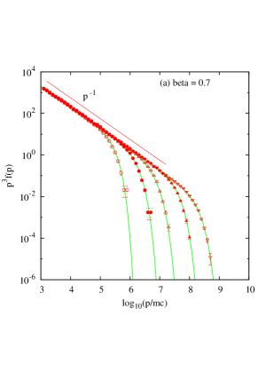
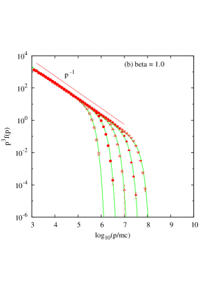
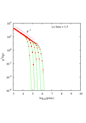
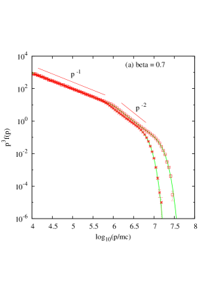
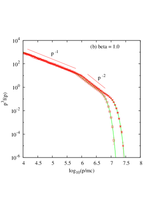
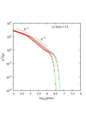
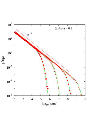
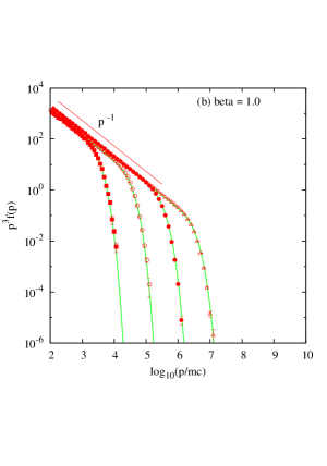
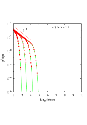
Figures 1, 2 and 3 show results of numerical simulation for the age-limited, cooling-limited and escape-limited cases, respectively. The spectra in these figures are for all particles which are still in the system at $t_{\rm age}$, that is,

$$F(p)\propto p^{3}f(p)\propto\int_{-x_{\rm feb}}^{\infty}F(x,u,t_{\rm age})\,dx~{}~{}.$$ (39)

The value $F$ of the distribution function for given momentum range $[u,u+\Delta u]$ is derived by an ensemble average. If injected particles with momentum $p_{\rm inj}$ have a statistical weight of unity, then, particles which have experienced splitting $n$ times have the statistical weight $w^{-n}$. Hence, we obtain

$$F=\sum_{\rm particles}w^{-n}~{}~{},$$ (40)

where summation is taken for all (split) particles which have a momentum between $u$ and $u+\Delta u$. Error bars in spectra of figures 1–3 are calculated assuming Poisson statistics. Taking into account the propagation of errors, the statistical error $\Delta F$ for given momentum range $[u,u+\Delta u]$ is calculated as

$$(\Delta F)^{2}=\sum_{\rm particles}w^{-2n}~{}~{}.$$ (41)

We adopt different values of $u_{\rm s1}$, $n_{\rm max}$ and $w$ for different runs so as to obtain good statistics near the maximum momentum (see Appendix). Therefore, for different runs, the length of error bars is different from each other. For each case, the dependence of the cutoff shape of the electron spectrum on $\beta$ is discussed below.

Figure 1: Electron spectra in the age-limited cases with (a) $\beta=0.7$ (Runs A07-1, A07-2, A07-3, A07-4, A07-5 from left to right), (b) $\beta=1.0$ (Runs A10-1, A10-2, A10-3, A10-4, A10-5 from left to right) and (c) $\beta=1.5$ (Runs A15-1, A15-2, A15-3, A15-4, A15-5 from left to right). Lines indicate the best fitted models described by equation (42).

Figure 2: Electron spectra in the cooling-limited cases with (a) $\beta=0.7$ (Runs C07-1, C07-2 from left to right), (b) $\beta=1.0$ (Runs C10-1, C10-2 from left to right) and (c) $\beta=1.5$ (Runs C15-1, C15-2 from left to right). Lines indicate the best fitted models described by equations (44), (45) and (46).

Figure 3: Electron spectra in the escape-limited cases with (a) $\beta=0.7$ (Runs E07-1, E07-2, E07-3, E07-4 from left to right), (b) $\beta=1.0$ (Runs E10-1, E10-2, E10-3, E10-4 from left to right) and (c) $\beta=1.5$ (Runs E15-1, E15-2, E15-3, E15-4 from left to right). Lines indicate the best fitted models described by equation (47).

3.3.1 Age-limited case: $p_{\rm m,age}<{\rm min}\{p_{\rm m,cool},p_{\rm m,esc}\}$

For each value of $\beta$ (0.7, 1.0 and 1.5), we had five runs with different $t_{\rm age}$. One can see from figure 1 that at lower electron momentum where $p\ll p_{\rm m,age}$, the spectrum is well described by the analytical solution in the steady state, $F(p)=p^{3}f(p)\propto p^{-1}$. Furthermore, estimated values of $p_{\rm m,age}$ (see Table 1) using equation (34) agree with the simulation result. Hence our present numerical scheme works well.

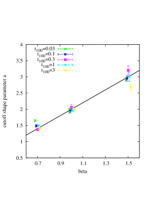
For all runs of age-limited acceleration, we have fitted the spectrum by the following function

$$F(p)\propto p^{-1}\exp\left[-\left(\frac{p}{p_{\rm m}}\right)^{a}\right]~{}~{},$$ (42)

and obtain the value of cutoff shape parameter $a$. The left panel of figure 4 shows the result. One can roughly confirm earlier result of numerical simulations, $a\approx 2\beta$ (Kato & Takahara, 2003; Kang et al., 2009).

Figure 4: Cutoff shape parameter $a$ as a function of $\beta$ in the age-limited (left), cooling-limited (center) and escape-limited (right) cases. The values of $a$ are derived by fitting the simulated spectra with the model described by equations (42) and (44) for age-limited and cooling-limited cases, respectively. Note that for escape-limited cases, we use phenomenological formula, equation (42), to derive values of $a$, while we used in Figure 3 the analytical stationary solution, equation (47), to fit the simulated spectra. In the left panel, data points are artificially shifted a little in the horizontal direction in order to be separated with each other and to be seen clearly. Solid lines represent $a=2\beta$, $a=\beta+1$ and $a=\beta$ for the age-limited, cooling-limited and escape-limited cases, respectively. The dashed line in the right panel shows $a=\beta+0.5$.

3.3.2 Cooling-limited case: $p_{\rm m,cool}<{\rm min}\{p_{\rm m,age},p_{\rm m,esc}\}$

For each value of $\beta$ (0.7, 1.0 and 1.5), we performed two simulations with the magnetic field strength of $B=2$ mG and 0.5 mG. Since the magnetic field strength $B$ is much larger than any other cases, the requirement for time step, equation (17), is the most severe, so that we set larger $p_{\rm inj}$ of $10^{4}m_{e}c$ in order to save the computation time.

In all runs, one can identify the cooling break, at which the spectral slope changes from $p^{-1}$ to $p^{-2}$. The break energy $p_{\rm b}$ is determined by the condition $t_{\rm cool}\approx t_{\rm age}$ (Longair, 2011), and we derive

$$p_{\rm b}\approx 2.45\times 10^{11}B_{\mu{\rm G}}^{-2}t_{100}^{-1}m_{e}c~{}~{}.$$ (43)

For example, we obtain from this equation $p_{\rm b}=6.1\times 10^{5}m_{e}c$ for run C07-1, which is consistent with the simulation result. In some runs such as C15-1 and C15-2, we can see pile-ups at the high-energy end (see the right panel of figure 2). Based on these facts, we fit spectra which were derived from simulations by the following function

$$F(p)\propto p^{-1}\,C_{\rm b}(p)\,C_{\rm p}(p)\,\exp\left[-\left(\frac{p}{p_{\rm m}}\right)^{a}\right]~{}~{},$$ (44)

where

$$C_{\rm b}(p)=\left[1+\left(\frac{p}{p_{\rm b}}\right)^{w}\right]^{-1/w}~{}~{},$$ (45)

and

$$C_{\rm p}(p)=\left[1+\left(\frac{p}{\eta p_{\rm m}}\right)^{q}\right]^{k/q}~{}~{},$$ (46)

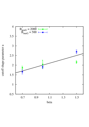
describe the cooling break and the pile-up effect, respectively. Middle panel of figure 4 shows the fitted $a$ as a function of $\beta$. The result is roughly consistent with the analytical result, $a=\beta+1$, which is derived on the steady state assumption (Zirakashvili & Aharonian, 2007; Yamazaki et al., 2013). In the case of $\beta=1.5$, fitted value of $a$ deviates from the analytical expectation of 2.5. This comes from the appearance of pile-up, which deforms the spectrum around the maximum momentum. Hence, it is implied that the analytical expectation $a=\beta+1$ is not always hold when the electron pile-up becomes significant.

Previously, based on similar numerical simulation to ours, Marcowith & Casse (2010) numerically obtain the shock front energy spectra, $F_{0}(p)=F(x=0,p)$, for the cases of $\beta=0$, 1/2 and 1, and confirmed the relation $a=\beta+1$ (for smaller dynamic range of momentum than ours). In the present study, we find that at least $\beta<1$, the relation $a=\beta+1$ roughly holds even for the spectrum of the whole region.

3.3.3 Escape-limited case: $p_{\rm m,esc}<{\rm min}\{p_{\rm m,age},p_{\rm m,cool}\}$

In this case, steady-state spectrum at the shock front ($x=0$) has been analytically derived as (Caprioli et al., 2009b; Reville et al., 2009; Yamazaki et al., 2013)

$$F_{0}(p) = F(x=0,p)$$ (47)

$$\propto p^{3}\exp\left[-\frac{4}{\beta}\int^{y(p)}\frac{{\rm d}\,\log y}{1-e^{-1/y}}\right]~{}~{},$$

where $y(p)=(p/p_{\rm m})^{\beta}$. For each value of $\beta$ (0.7, 1.0 and 1.5), we have four runs with different $x_{\rm feb}$. Then, we find that in all runs, the derived spectra are well fitted with models described by equation (47) (see figure 3). Hence, equation (47) well reproduces the spectrum of the whole region with good accuracy although it has been derived as the shock front spectrum at $x=0$.

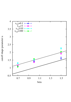
Here we discuss on whether the simulated spectra are fitted with phenomenological formula, equation (42). In the limit $p\gg p_{\rm m}$, we can approximate $1-e^{-1/y}\approx 1/y$ in equation (47), resulting in $F_{0}(p)\propto\exp[-(p/p_{\rm m})^{\beta}]$, so that one might expect $a=\beta$ (Yamazaki et al., 2013). If we fit numerically derived spectra with equation (42), then the fitted values of $a$ are not along with the expectation $a=\beta$. Difference between equations (47) and (42) with $a=\beta$ is large at $p\sim p_{\rm m}$. However, they seem to lie on $a\approx\beta+0.5$ (see the right panel of figure 4). This implies that $F(p)\propto p^{-1}\exp[-(p/p_{\rm m})^{\beta}]$ is not a good approximation around the maximum momentum $p_{\rm m}$.

4 Summary and Discussion

We have developed a numerical method of SDE to simulate electron acceleration at astrophysical shocks. Our code involves Zhang’s method of skew Brownian motion and particle splitting. Using this code, we have performed simulations of electron acceleration at stationary plane parallel shock, and we reproduced the analytical result in the momentum range much smaller than the maximum momentum — $f(p)\propto p^{-4}$ in the age-limited and escape-limited cases, and the broken power-law which changes from $f(p)\propto p^{-4}$ to $p^{-5}$ at the cooling break in the cooling-limited cases. These results can be achieved due to incorporation of Zhang’s method. Furthermore, the maximum electron momentum in the simulated spectra can be well explained by simple analytical argument, which is the outcome of the particle splitting method. Therefore, we believe our numerical code works well, and it enables us to study the cutoff shape of the electron spectrum.

We have performed simulations for various parameter sets, and studied how the cutoff shape, which is characterized by cutoff shape parameter $a$, changes with the momentum dependence of the diffusion coefficient $\beta$. In the age-limited cases, we have reproduced previous results of other authors, $a\approx 2\beta$. In the cooling-limited cases, the analytical expectation $a\approx\beta+1$ is roughly reproduced although we recognize deviations to some extent (runs C15-1 and C15-2) when the pile-up effect is significant. However, we have found in the Bohm type diffusion, $K\propto p$ and $\beta=1$, the cutoff shape parameter $a$ is consistent with the analytical prediction $a=2.0$ both in the age-limited and cooling-limited cases. Hence, if the effect of escape can be neglected, $a=2$ should be canonical value. Note that in the present study, we have assumed plane shock geometry and constant electron injection. In reality, the SNR shock is nearly spherical although it has fluctuation (e.g., Inoue et al., 2012). In the spherical shock case, accelerated particles downstream of the shock experience adiabatic losses. This reduces the mean energy gain they experience at the shock, which steepens the spectral slope (e.g., Yamazaki et al., 2006; Schure et al., 2010). In addition, the exact spectral slope in a time-dependent calculation depends on the injection history, which may be complicated depending on the shock velocity, ambient density and so on. These effects may influence the electron spectrum. However, we are currently interested in the energy region near the upper end of the spectrum. At the given epoch, the spectrum around the maximum energy is dominated by those which are being accelerated at that time because previously accelerated particles have suffered the adiabatic losses during transported downstream of the shock. Hence, one can expect that the cutoff shape of the spectrum does not so much depend on the past acceleration history (Yamazaki et al., 2006, 2013). This issue has not yet been studied in detail except for a few works in which the spherical and planar shock cases were compared (Schure et al., 2010; Kang, 2015), and should be investigated more in future works.

The maximum momentum is sometimes determined by the escape of accelerated particles upstream. In this case, we should use the functional form given by equation (47), otherwise we should use (42) with $a=\beta+0.5$. Electron acceleration at SNRs is sometimes limited by the escape (see figure 1 and 2 of Ohira et al., 2012), as well as proton acceleration, which might be inferred by recent gamma-ray observation (e.g., Ohira et al., 2010). In the present study we adopt weak magnetic field in all runs of the escape-limited cases, so that synchrotron cooling effect can be neglected. Hence, our result for the escape-limited cases is applicable to the proton acceleration. The cutoff shape around the maximum proton momentum may be studied by the precise gamma-ray spectrum which will be taken in the near future.

In the present study, we have used the test particle approximation, neglecting feedback of the accelerated particles on to the plasma forming background shock structure. Not electrons but protons deform the background plasma, because they are coupled with each other through the waves excited by accelerated protons themselves. Various authors focus on the feedback processes of accelerated particles on to the magnetohydrodynamic properties around the shock. (e.g., Berezhko & Ellison, 1999; Malkov & Drury, 2001; Kang & Jones, 2005; Vladimirov et al., 2006; Terasawa et al., 2007; Caprioli et al., 2009a; Yamazaki et al., 2009; Zirakashvili & Ptuskin, 2012; Bykov et al., 2014). In such cosmic-ray modified shocks, electron acceleration is also affected by the shock deformation, and the results may be different from those in the test particle limit. These studies are remained as a future work.

Appendix: Parameters for numerical simulation

Parameters for numerical simulation are summarized in Table 2. Time step, $\Delta t$, must satisfy the condition (17). In the present study, it is taken to be smaller than $2K_{1}(p_{\rm inj})/v_{1}^{2}$.

We need four parameters, $u_{\rm s0}$, $u_{\rm s1}$, $n_{\rm max}$ and $w$, to carry out particle splitting. In the present study, we set $u_{\rm s0}=\ln(p_{\rm inj}/m_{e}c)$. The other parameters are taken differently for each run.

Table 2: Adopted parameters in the present study.

Run	$\Delta t$	$n_{\rm max}$	$w$	$p_{\rm s1}$
	[$10^{3}$s]			[$m_{e}c$]
A07-1	10	6	12	$10^{9.0}$
A07-2	10	6	12	$10^{9.0}$
A07-3	10	6	12	$10^{9.0}$
A07-4	10	6	12	$10^{9.0}$
A07-5	10	6	12	$10^{9.0}$
A10-1	10	6	12	$10^{8.0}$
A10-2	10	6	12	$10^{8.0}$
A10-3	10	6	12	$10^{8.0}$
A10-4	10	6	12	$10^{8.0}$
A10-5	10	6	12	$10^{8.0}$
A15-1	1	6	12	$10^{9.0}$
A15-2	1	6	12	$10^{9.0}$
A15-3	1	6	12	$10^{9.0}$
A15-4	1	6	12	$10^{9.0}$
A15-5	1	6	12	$10^{9.0}$
C07-1	5	5	10	$10^{6.5}$
C07-2	8	5	10	$10^{6.5}$
C10-1	0.5	5	10	$10^{6.5}$
C10-2	1	5	10	$10^{7.0}$
C15-1	0.8	5	10	$10^{6.5}$
C15-2	3.2	5	10	$10^{6.5}$
E07-1	0.11	6	10	$10^{6.0}$
E07-2	0.11	6	10	$10^{6.0}$
E07-3	0.11	6	10	$10^{7.0}$
E07-4	0.11	6	10	$10^{7.0}$
E10-1	0.11	6	10	$10^{6.0}$
E10-2	0.11	6	10	$10^{6.0}$
E10-3	0.11	6	10	$10^{6.0}$
E10-4	0.11	6	10	$10^{6.0}$
E15-1	0.11	5	4	$10^{2.5}$
E15-2	0.11	6	10	$10^{5.5}$
E15-3	0.11	6	10	$10^{5.5}$
E15-4	0.11	6	10	$10^{5.5}$

References

- Achterberg & Krülls (1992) Achterberg, A. & Krülls, W. M. 1992, A&A, 265, L13
- Achterberg & Schure (2011) Achterberg, A. & Schure, K. M. 2011, MNRAS, 411, 2628
- Actis et al. (2011) Actis, M., Agnetta, G., Aharonian, F., et al. 2011, Experimental Astronomy, 32, 193
- Bamba et al. (2003) Bamba, A. et al. 2003, ApJ, 589, 827
- Bamba et al. (2005a) Bamba, A. et al. 2005a, ApJ, 621, 793
- Bamba et al. (2005b) Bamba, A. et al. 2005b, ApJ, 632, 294
- Bell (1978) Bell, A. R. 1978, MNRAS, 182, 147
- Berezhko & Ellison (1999) Berezhko E. G., Ellison D. C., 1999, ApJ, 526, 385
- Blandford & Ostriker (1978) Blandford, R. D., & Ostriker, J. P. 1978, ApJ, 221, L29
- Bykov et al. (2014) Bykov, A. M. et al. 2014, ApJ, 789, 137
- Caprioli et al. (2009a) Caprioli, D., Blasi, P., & Amato, E. et al. 2009a, MNRAS, 396, 895
- Caprioli et al. (2009b) Caprioli, D., Blasi, P., & Amato, E. 2009b, MNRAS, 396, 2065
- Drury (1983) Drury, L. O’C., 1983, Rep. Prog. Phys., 46, 973
- Gardiner (1983) Gardiner, C. W. 1983, Handbook of Stochastic Differential Equations (Princeton: Princeton Univ. Press)
- Hailey et al. (2010) Hailey, C. J., An, H., Blaedel, K. L., et al. 2010, in Society of Photo-Optical Instrumentation Engineers (SPIE) Conference Series, 7732, 77320T
- Harrison et al. (2013) Harrison, F. A., Craig, W. W., Christensen, F. E., et al. 2013, ApJ, 770, 103
- Harrison & Shepp (1981) Harrison, J. M. & Shepp, L. A. 1981, Ann. Probability, 9, 309
- Inoue et al. (2012) Inoue, T., Yamazaki, R., Inutsuka, S. et al. 2012, ApJ, 744, 71
- Kang (2015) Kang, H. 2015, J. Korean Astron. Soc., in press (arXiv:1411.7513)
- Kang & Jones (2005) Kang, H., Jones T. W., 2005, ApJ, 620, 44
- Kang et al. (2009) Kang, H., Ryu, D., & Jones, T. W. 2009, ApJ, 695, 1273
- Kato & Takahara (2003) Kato, T. N., & Takahara, F. 2003, MNRAS, 342, 639
- Krülls & Achterberg (1994) Krülls, W. M. & Achterberg, A. 1994, A&A, 286, 314
- Krymskii (1977) Krymskii, G. F. 1977, Akademiia Nauk SSSR Doklady, 234, 1306
- Longair (2011) Longair, M. S. 2011, High energy astrophysics (Cambridge: Cambridge Univ. Press), section 16.3.1, p. 540
- Malkov & Drury (2001) Malkov, M. A., & O’C Drury, L. 2001, Reports on Progress in Physics, 64, 429
- Marcowith & Casse (2010) Marcowith, A. & Casse, F. 2010, A&A, 515, A90
- Marcowith & Kirk (1999) Marcowith, A. & Kirk, J. G. 1999, A&A, 347, 391
- Ohira et al. (2010) Ohira, Y., Murase, K. & Yamazaki, R. 2010, A&A, 513, A17
- Ohira et al. (2012) Ohira, Y., Yamazaki, R., Kawanaka, N. et al. 2012, MNRAS, 427, 91
- Reville et al. (2009) Reville, B., Kirk, J. G., & Duffy, P. 2009, ApJ, 694, 951
- Schure et al. (2010) Schure, K. M. et al. 2010, MNRAS, 406, 2633
- Takahashi et al. (2010) Takahashi, T., Mitsuda, K., Kelley, R., et al. 2010, in Society of Photo-Optical Instrumentation Engineers (SPIE) Conference Series, 7732, 77320Z
- Terasawa et al. (2007) Terasawa, T. et al. 2007, Prog. Theor. Phys. Suppl., 169, 146
- Uchiyama et al. (2007) Uchiyama, Y. et al. 2007, Nat, 449, 576
- Vink & Laming (2003) Vink, J. & Laming, J. M. 2003, ApJ, 584, 758
- Vladimirov et al. (2006) Vladimirov A., Ellison D. C., Bykov A., 2006, ApJ, 652, 1246
- Yamazaki et al. (2004) Yamazaki, R. et al. 2004, A&A, 416, 595
- Yamazaki et al. (2006) Yamazaki, R. et al. 2006, MNRAS, 371, 1975
- Yamazaki et al. (2009) Yamazaki, R., Kohri, K., & Katagiri, H. 2009, A&A, 495, 9
- Yamazaki et al. (2013) Yamazaki, R., Ohira, Y., Bamba, A., & Sawada, M. 2013, Res. Astron. Astrophys., 14, 165 (arXiv:1301.7499)
- Yoshida & Yanagita (1994) Yoshida, T. & Yanagita, S. 1994, PTP, 92, 1217
- Yoshida & Yanagita (1997) Yoshida, T. & Yanagita, S. 1997, Proc. 2nd INTEGRAL Workshop ‘The Transparent Universe’, ESA SP-382, 85
- Zhang (2000) Zhang, M. 2000, ApJ, 541, 428
- Zirakashvili & Aharonian (2007) Zirakashvili, V. N., & Aharonian, F. 2007, A&A, 465, 695
- Zirakashvili & Ptuskin (2012) Zirakashvili, V. N., & Ptuskin, V. S. 2012, Astropart. Phys., 39, 12