Mesoscopic superpositions of Tonks-Girardeau states and the Bose-Fermi mapping

Abstract

We study a one dimensional gas of repulsively interacting ultracold bosons trapped in a double-well potential as the atom-atom interactions are tuned from zero to infinity. We concentrate on the properties of the excited states which evolve from the so-called NOON states to the NOON Tonks-Girardeau states. The relation between the latter and the Bose-Fermi mapping limit is explored. We state under which conditions NOON Tonks-Girardeau states, which are not predicted by the Bose-Fermi mapping, will appear in the spectrum.

The recent ground-breaking experiments on the trapping of a few fermions or bosons have stir up the theoretical interest in small ultracold quantum gases 2010XeOE ; 2011SerwaneScience ; 2012ZurnPRL ; 2013WenzScience ; 2013BourgainPRA ; 2014PaganoNatphys . The atoms in these experiments can be often regarded as being effectively trapped in one dimension and interacting through contact interactions. This is a system with many examples of exact solvability (see, e.g., 2008GiorginiRMP ; 2011CazalillaRMP ; 2013GuanRMP ). A step forward in these experiments is to consider other geometries, a goal which is already accomplished for double-well potentials 2014MurmannArxiv .

Experiments have already reached the strongly interacting 1D gas of bosons Kinoshita ; Paredes , exploring the mapping of repulsive bosons into a system of ideal fermions to form the so-called Tonks-Girardeau (TG) gas Girardeau1960 ; Girardeau2001 . Simultaneously, double-well experiments with ultracold bosons 2005AlbiezPRL ; 2007LevyNature should sooner than later allow one to produce macroscopic superpositions 1998CiracPRA . So, combining the two may allow one to produce macroscopic superpositions of strongly interacting TG gases. In this letter we settle under which conditions the superpositions in the Fock regime, so called NOON (cat-like) states 2009WeissPRL ; 2009StreltsovPRA ; 2013FogartyPRA , evolve into superpositions of TG gases, termed NOON TG, as the interactions are tuned from small to infinity.

Model Hamiltonian.

Let us consider $N$ atoms trapped in a one-dimensional double-well potential, described by the first-quantized Hamiltonian $\hat{H}=\sum_{j=1}^{N}\left[-(1/2)\partial^{2}_{z_{j}^{2}}+V_{\rm{DW}}(z_{j})\right]+V_{\rm int}$, where the interaction is taken as a contact, $V_{\rm int}=g\sum_{i<j}\delta(z_{i}-z_{j})$ and where $\hbar=m=1$. To model the double-well potential we use a simplified Duffing potential, $V_{\mathrm{DW}}(z)=V_{0}\left(-8(z/V_{0})^{2}+16(z/V_{0})^{4}+1\right)$. This Duffing potential has two minima equal to zero at $z=\pm V_{0}/2$ and a local maximum equal to $V_{0}$ at $z=0$. $V_{0}$ is thus the barrier height and the distance between the wells. In our study, we take $V_{0}\in[V_{0}^{\mathrm{min}},V_{0}^{\mathrm{max}}]$, with $V_{0}^{\mathrm{min}}$ a small number and $V_{0}^{\mathrm{max}}$ large enough to get a degeneracy of the order of $10^{-10}$ between the first two single-particle eigenstates (that is $V_{0}^{\mathrm{max}}\simeq 12$). By increasing $V_{0}$, the confining potential goes from a quartic, for $V_{0}\to 0$, into increasingly deeper double-well potentials. Let $\phi_{n}$ be the $n$-th eigenstate of the single-particle Hamiltonian $H_{\mathrm{sp}}=(1/2)\partial^{2}_{z^{2}}+V_{\mathrm{DW}}(z)$ with energy $\varepsilon_{n}$. As $V_{0}$ is increased, quasi-degeneracies between the single-particle energies are introduced, see Fig. 1(a). These occur for values of the corresponding quasi-degenerate pair of energies smaller than $V_{0}$.

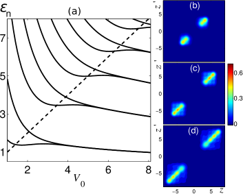
Figure 1: (a) The first ten eigenvalues of the single-particle Hamiltonian as a function of $V_{0}$ are depicted. The dashed line represents the condition $E=V_{0}$. (b)-(d) One-body density matrix for NOON Tonks-Girardeau states of $N=2,3$ and 4 obtained with $V_{0}=6,10$ and 12, respectively.

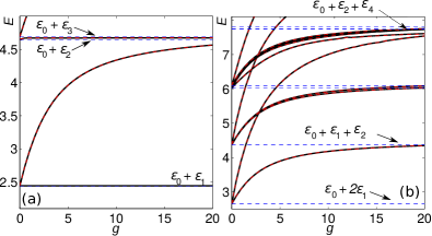
Figure 2: Energy spectra for $N=2$ (a) and $N=3$ (b) with $V_{0}=5$ and $V_{0}=10$, respectively. The blue dashed lines in both panels represent the energies expected in the Fermionized limit, $g\to\infty$ (we explicitly label a few of them to help to understand this limit). These energies have been calculated by extrapolating the results obtained with an increasing number of modes, with a maximun number of modes of 30 and 24 for $N=2$ and $N=3$, respectively.

Spinless fermions.

For $N$ spinless fermionic atoms, the ground and all excited states $\Psi^{\rm f}_{k}$ of $\hat{H}$ are Slater determinants built up from $N$ single-particle eigenstates $\phi_{n}$. This wave functions fulfil the Pauli exclusion principle, i.e. are zero whenever $z_{i}=z_{j}$, and therefore do not feel the contact interaction potential. Also, these solutions have a sign change at these points, i.e. for fermions, the wavefunction has to change sign when an atom of coordinate $z_{i}$ is interchanged with one at $z_{j}$. The energies of the many-body eigenstates $\Psi^{\rm f}_{k}$ are the summation of the energies of the single-particle states used to build the corresponding Slater determinant.

For $N=2$ fermions, which will be used as a limiting case in the forthcoming discussions, the ground state is $\Psi^{\rm f}_{0}(z_{1},z_{2})=1/\sqrt{2}\,{\rm Slater}(\phi_{0},\phi_{1})=1/\sqrt{2}\left(\phi_{0}(z_{1})\phi_{1}(z_{2})-\phi_{1}(z_{1})\phi_{0}(z_{2})\right)$ and has energy $E_{0}=\varepsilon_{0}+\varepsilon_{1}$ for all $V_{0}$. For large $V_{0}$, the first two single-particle states are quasi-degenerate, $\varepsilon_{1}=\varepsilon_{0}+\varepsilon_{01}$, with $\varepsilon_{01}\ll\varepsilon_{0}$. The next four excited states are $\Psi^{\rm f}_{1}\sim{\rm Slater}(\phi_{0},\phi_{2})$, $\Psi^{\rm f}_{2}\sim{\rm Slater}(\phi_{1},\phi_{2})$, $\Psi^{\rm f}_{3}\sim{\rm Slater}(\phi_{0},\phi_{3})$, and $\Psi^{\rm f}_{4}\sim{\rm Slater}(\phi_{1},\phi_{3})$. For $V_{0}\gtrsim 4.5$, the second and third single-particle states are also quasi-degenerate (see Fig. 1), and therefore their energies can be written as $\varepsilon_{3}=\varepsilon_{2}+\varepsilon_{23}$, with $\varepsilon_{23}\ll\varepsilon_{2}$. Thus, for $V_{0}\gtrsim 4.5$ the first four excited states are quasidegenerate and have energies $E_{1}=\varepsilon_{0}+\varepsilon_{2}$, $E_{2}=\varepsilon_{0}+\varepsilon_{2}+\varepsilon_{01}$, $E_{3}=\varepsilon_{0}+\varepsilon_{2}+\varepsilon_{23}$, and $E_{4}=\varepsilon_{0}+\varepsilon_{2}+\varepsilon_{01}+\varepsilon_{23}$. For two atoms, the next excited state has a finite energy gap with this manifold (see gap between $\varepsilon_{3}$ and $\varepsilon_{4}$ for large $V_{0}$ in Fig. 1).

For sufficiently large $V_{0}$, such that a sizeable amount of pairs of single-particle states are quasidegenerate, we can define the following single-particle wavefunctions,

$$\phi_{n}^{j}=\left\{\begin{array}[]{@{}c@{\quad}l@{}}\phi_{n}^{L}=\dfrac{1}{\sqrt{2}}(\phi_{2n}+\phi_{2n+1})&\\ \phi_{n}^{R}=\dfrac{1}{\sqrt{2}}(\phi_{2n}-\phi_{2n+1})&\,,n=0,1,\dots\,.\\ \end{array}\right.$$ (1)

Here $j=L(R)$ stands for left (right). These $\phi_{n}^{j}$ functions are mostly localized either in the left or right well when the pair of delocalized functions $\phi_{n}$ used to construct them are quasi-degenerate. For large interaction energies, the small degeneracy breaking between the states will in some cases become irrelevant, and a much simpler picture is obtained in the localized basis.

Interacting bosons in a double well.

Using the single-particle eigenfunctions to build the Fock basis, the many-body Hamiltonian for bosons reads

$$\mathcal{\hat{H}}=\sum_{i=1}^{M}\varepsilon_{i}\hat{a}_{i}^{\dagger}\hat{a}_{i}+\dfrac{g}{2}\sum_{k,l,m.n}^{M}I_{k,l,m,n}\hat{a}_{k}^{\dagger}\hat{a}_{l}^{\dagger}\hat{a}_{m}\hat{a}_{n},$$ (2)

with $I_{k,l,m,n}=\int dz\phi_{k}(z)\phi_{l}(z)\phi_{m}(z)\phi_{n}(z)$, where $[\hat{a}_{k}^{\dagger},\hat{a}_{i}]=\delta_{ik}$ and $[\hat{a}_{k}^{\dagger},\hat{a}_{i}^{\dagger}]=\left[\hat{a}_{k},\hat{a}_{i}\right]=0$. A Fock vector is written as $|n_{0},n_{1},\dots n_{M}\rangle={\cal N}(a^{\dagger}_{0})^{n_{0}}\dots,(a^{\dagger}_{M})^{n_{M}}|{\rm vac}\rangle$, where $|{\rm vac}\rangle$ is the vacuum, $n_{i}$ is the number of atoms in mode $i$ and ${\cal N}^{-1}=\sqrt{n_{0}!\dots n_{M}!}$.

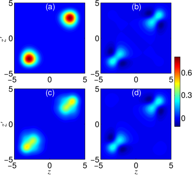
Figure 3: One-body density matrices of two of the four excited states for two bosons in a double-well for $V_{0}=5$. The upper (lower) row is computed with $g=0.5$ ($g=20$). One-body density matrices for a NOON state, panel (a), and its evolved state, panel (c), and a non-interacting state, panel (b) and its evolved state, panel (d).

Beyond the bimodal Fock regime.

For small interactions the system remains bimodal, allowing to explore with a two-mode model from the Josephson to the Fock regimes2001LeggetRMP ; 2012DaltonJMO . As interactions are increased, the system approaches the strongly correlated regime 2004StreltsovPRA ; 2008MurphyPRA ; 2008ErnstPRA . Let us explore in detail this transition, using as driving examples the $N=2$ and $N=3$ cases.

Assuming a barrier high enough to have two quasi-degenerate pairs in the lower part of the single-particle spectrum, the interaction energy will make the energy gaps irrelevant. In this case, the simplest picture is provided using the localized single-particle basis defined in Eq. (1). Using this basis, the Fock vectors can be written as, $|n_{0}^{L},n_{0}^{R},n_{1}^{L},n_{1}^{R},\dots\rangle_{\rm lo}={\cal N}(a^{L\,\dagger}_{0})^{n_{0}^{L}}(a^{R\,\dagger}_{0})^{n_{0}^{R}}\dots(a^{L\,\dagger}_{M/2})^{n_{M/2}^{L}}(a^{R\,\dagger}_{M/2})^{n_{M/2}^{R}}|{\rm vac}\rangle$ with ${\cal N}^{-1}=\sqrt{n_{0}^{R}!n_{0}^{L}!\ \dots n_{M/2}^{R}!n_{M/2}^{L}!}$.

For instance, in the $N=2$ case, once the interaction is larger than the gap, the ground state is well approximated by $|1,1,0,\dots\rangle_{\rm lo}$. This state has one atom in each well and is thus unaffected by the interaction. Its energy remains constant as $g$ is increased, see Fig. 2(a). The first two excited states, quasidegenerated with the ground state in the non-interacting case, are the NOON states, $|{\rm NOON}_{2}\rangle=(|0,2,0,\dots\rangle_{\rm lo}\pm|2,0,0,\dots,\rangle_{\rm lo})/\sqrt{2}$, which contain a delocalized pair of interacting atoms (two atoms in the same well). Their energy grows linearly with $g$ for small $g$, see Fig. 2(a). The next excited states involve more than two modes and are clearly gapped in absence of interactions 2007DounasFrazerPRL ; 2012GarciaMarchFiP . They read, $(|0,1,1,0,\dots\rangle_{\rm lo}\pm|1,0,0,1,0,\dots\rangle_{\rm lo})/\sqrt{2}$, and $(|0,1,0,1,0,\dots\rangle_{\rm lo}\pm|1,0,1,0,\dots\rangle_{\rm lo})/\sqrt{2}$. As before, the first two are mostly non-interacting and thus their energies remain constant as $g$ is increased. The latter, however, have one pair of interacting atoms, their energy grows linearly with similar slope as the $|{\rm NOON}_{2}\rangle$ states, see Fig. 2(a).

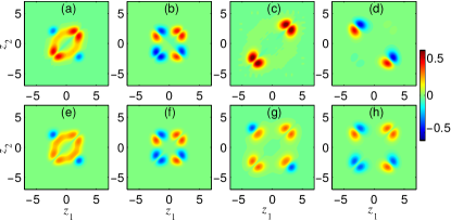
Figure 4: Comparison of two of the four excited numerical wave functions for $g=20$ (upper row) and the analytic ones $\Psi^{\rm b}_{1}$ (e,g) and $\Psi^{\rm b}_{3}$ (f,h) obtained through the Bose-Fermi mapping (lower row). Panels (a), (b), (e) and (f) are obtained with $V_{0}=4$, while panels (c), (d), (g) and (h) correspond to $V_{0}=5$. $N=2$.

For $N>2$ there are no noninteracting states. For $N=3$ the lowest energy manifold at small interactions is $(|1,2,0,\dots\rangle_{\rm lo}\pm|2,1,0,\dots,\rangle_{\rm lo})$ and the NOON states, $|{\rm NOON}_{3}\rangle=(|3,0,0,\dots\rangle_{\rm lo}\pm|0,3,0,\dots,\rangle_{\rm lo})$. The pair of atoms on the same well in the first ones are responsible for the linear increase in the energy as a function of $g$, with same slope as for $N=2$ discussed above. In contrast, the NOON states have 3 interacting pairs, with a correspondingly larger slope, see Fig. 2(b).

In the general case, the lowest energy manifold at small $g$ is $|N,0,0,\dots\rangle_{\rm lo}\pm|0,N,0,\dots\rangle_{\rm lo}$, $|1,N-1,0\dots\rangle_{\rm lo}\pm|N-1,1,0\dots\rangle_{\rm lo}$, etc. Our interest at this point is to disentangle the fate of these states as the interaction is varied from the Fock regime into the strongly interacting regime. In particular, what happens with the states in which more than one atom populates each well in the Fock regime. The driving intuition is twofold. On one hand, we know that for bosons in a single well, the system evolves into a TG gas, i.e. the NOON would directly evolve into a NOON TG gas. On the other hand, the Bose-Fermi mapping theorem can be directly applied to the system, providing exact solutions in the infinitely interacting case, which will be shown to be in contradiction with the first one.

From NOON to the NOON Tonks-Girardeau.

The $N=2$ and $N=3$ cases are again very illustrative. We note that energetically the fate of the NOON states in $N=2$ is very similar to what happens to the $(|1,2,0,\dots\rangle_{\rm lo}\pm|2,1,0,\dots\rangle_{\rm lo})/\sqrt{2}$ states in $N=3$, see Fig. 2, i.e. the third particle in the $N=3$ plays an spectator role as $g$ is increased. The latter takes place also in the general $N>2$ case, where none of the eigenstates is non-interacting and in which upon increasing $g$ the system is expected to increase correlations to avoid the interaction. Thus, let us first disentangle the fate of the NOON states at $N=2$. From Fig. 2(a) we see that as $g$ is further increased, their energies saturate to a constant value which actually approaches $\varepsilon_{0}+\varepsilon_{2}$. This is also essentially the energy of the states evolved from $(|0,1,1,0,\dots\rangle_{\rm lo}\pm|1,0,0,1,0,\dots\rangle_{\rm lo})/\sqrt{2}$, which are non-interacting. Thus, in the strongly interacting regime, there are four quasi-degenerate states.

The evolution with increasing $g$ of their one-body density matrices (OBDM) is very telling. The NOON states, evolve from the $|{\rm NOON}_{2}\rangle$ states at $g=0.5$, see Fig. 3(a), to distributions with two peaks per well (or three and four peaks per well for $N=3$ and $N=4$, respectively, see Fig. 1(c,d)), resembling the OBDM for two TG gases, Fig. 3(c). The OBDM for the non-interacting states similarly shows two-peaks per well, as would correspond to populating the single-particle states $\phi_{2,3}$, which have one node in each well.

Let us now examine the prediction from the Bose-Fermi mapping theorem. The rigorous Bose-Fermi mapping theorem is established by noting that the bosonic problem in the $g\to\infty$ is equivalent to the fermionic problem when imposing the boundary condition that the wave functions have to vanish if $z_{j}=z_{j^{\prime}}$. This boundary condition is obeyed by the fermions for free because it is imposed by the Pauli exclusion principle. Then, the bosonic wave functions $\Psi^{\rm{b}}$ can be obtained from the fermionic ones $\Psi^{\rm{f}}$ after symmetrizing them, $\Psi^{\rm{b}}=A\Psi^{\rm{f}}\,\,\,\mbox{with}\,\,A=\prod_{j>j^{\prime}}\mbox{sgn}(z_{j}-z_{j^{\prime}})$, with $\mbox{sgn}(z)$ the sign function. The analytic form of the wave functions for the case of fermions was discussed above. The Bose-Fermi mapping theorem applies equally regardless of the value of $V_{0}$.

In Fig. 4 we compare the predictions of the Bose-Fermi mapping, to the actual numerical results, for $N=2$ and for $V_{0}=4$ and $V_{0}\gtrsim 4.5$. For $V_{0}=4$, the Bose-Fermi mapping, panels (e,f), provides an accurate representation of the numerically obtained results, panels (a,b). Both the NOON and the non-interacting states, evolve at $g=20$ to the states predicted by the Bose-Fermi mapping. Note that in this case, the barrier is not high enough to substantially localize the single-particle ground and first excited state, see Fig. 1. None of the many-body states is however a NOON TG state.

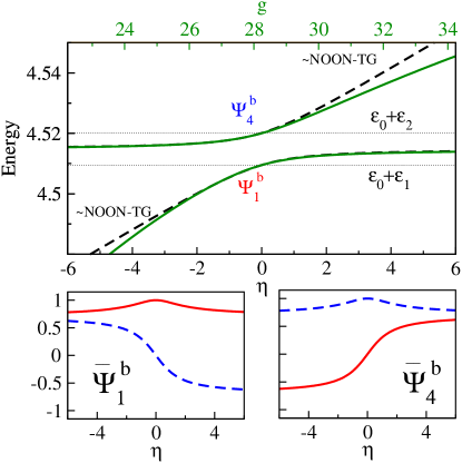
Figure 5: Detailed analysis of the $g\to\infty$ limit for $V_{0}=5.5$ (upper panel). Two of the first excited states for $N=2$ and $V_{0}$, computed numerically, solid lines, compared to the results of the perturbation theory when the width of the perturbation is $\sigma\simeq 0.07$ (see the text for further details), dashed lines. The small panels depict the composition of the dressed states, $\bar{\Psi}_{1}^{b}$ and $\bar{\Psi}_{4}^{b}$: $\langle\bar{\Psi}_{k}^{b}|\Psi_{1}^{b}\rangle$ (solid, red) and $\langle\bar{\Psi}_{k}^{b}|\Psi_{4}^{b}\rangle$ (dashed, blue). A similar qualitative picture is obtained for states $\bar{\Psi}_{2}^{b}$ and $\bar{\Psi}_{3}^{b}$.

A surprising result appears however as we increase the barrier height, going from $V_{0}=4$ to $V_{0}=5$ in Fig. 4. In this case, the prediction of the Bose-Fermi mapping, panels (g,h), and the numerical results, panels (c,d), clearly disagree. The numerical results show less left-right coherence than the Bose-Fermi prediction. That is, there is essentially zero probability of finding two bosons in the same well, as seen in Fig. 4 (d), while in the Bose-Fermi mapping, the probability is clearly non-negligible in all four states. It is worth mentioning that these differences, which involve pair-correlations, are not reflected in the density profiles, i.e., the diagonal of the one-body density matrices, Figs. 1(b,c,d) and 3 (c,d). What causes such discrepancy? And, more important, what would an experiment find? Let us note, that in all cases, the left-right symmetry is fully respected, i.e. it is not a consequence of spurious numerical biases in the numerics.

Finite-range effects.

The Bose-Fermi mapping applies for delta interaction potentials in the strict infinite interaction case. The Slater determinant ensures that the atoms do not interact, but, any finite size correction to the delta contact potential immediately implies a non-zero interaction between the two atoms. In addition, any numerical approach has an inherent minimal distance resolved, in our case related to the maximun number of modes considered. Thus, for any number of modes, if $g$ is sufficiently large, finite size corrections to the contact should show up. This energy stemming from the finite range of the atom-atom interaction, can be comparable to the splitting between the four excited states described above, resulting in a mixture of the four states.

This hypothesis can be tested quantitatively. Let us consider a finite range perturbation on the four states predicted by the Bose-Fermi mapping, e.g. $V_{\rm pert}(z_{j}-z_{j^{\prime}})=\eta/\sqrt{2\pi\sigma^{2}}\exp\left[-(z_{j}-z_{j^{\prime}})^{2}/(2\sigma^{2})\right]$, and diagonalize it in the restricted space spanned by $\{\Psi_{1}^{\rm b},\Psi_{2}^{\rm b},\Psi_{3}^{\rm b},\Psi_{4}^{\rm b}\}$. Then we obtain the dressed states $\{\bar{\Psi}_{1}^{\rm b},\bar{\Psi}_{2}^{\rm b},\bar{\Psi}_{3}^{\rm b},\bar{\Psi}_{4}^{\rm b}\}$. The perturbation theory prediction can be compared to the numerical results by noting that the $\eta=0$ corresponds to the value of $g$ for which the bose-fermi energies are reproduced for the number of modes used. As seen in Fig. 5 the model predicts a nice avoided crossing in agreement with the numerics. For $\eta<0$, thus removing repulsion from the $g\to\infty$ limit, we have the NOON TG as the lowest states of the manifold, $\bar{\Psi}^{\rm b}_{1}\simeq(\Psi^{\rm b}_{1}+\Psi^{\rm b}_{4})/\sqrt{2}$ (see Fig. 5) and $\bar{\Psi}^{\rm b}_{2}\simeq(\Psi^{\rm b}_{2}+\Psi^{\rm b}_{3})/\sqrt{2}$. For $\eta>0$, the repulsive finite size correction sets the non-interacting states $\bar{\Psi}^{\rm b}_{1}\simeq(\Psi^{\rm b}_{1}-\Psi^{\rm b}_{4})/\sqrt{2}$ and $\bar{\Psi}^{\rm b}_{2}\simeq(\Psi^{\rm b}_{2}-\Psi^{\rm b}_{3})/\sqrt{2}$ as the lowest in the manifold.

These results, checked for $N=2,3$ and $4$ are expected to remain valid for larger number of atoms. NOON states will evolve to NOON Tonks-Girardeau states provided two conditions are met: 1) the potential barrier has to be large enough to ensure the existence of $N$ quasi-degenerate doublets in the single-particle spectrum, and 2) the actual range of the contact interaction is non-zero but finite, which is what actually happens in an experiment, such that in the infinitely interacting limit the residual interaction mixes the corresponding states predicted by the Bose-Fermi mapping to produce NOON Tonks-Girardeau states. These findings, which require two-body correlations to be explicitly measured, will be of relevance in future experimental efforts to build strongly correlated states with inter-site spatial entanglement. As an outlook, we foresee that, for a general trapping potential with an associated single-particle eigenspectra showing quasidegeneracies, the effect of the finite range of the contact interactions may involve discrepancies between the result predicted by the Bose-Fermi mapping and the actual solution.

We acknowledge useful discussions with Prof. Thomas Busch. We acknowledge partial financial support from the DGI (Spain) Grant No. FIS2011-25275, FIS2011-24154 and the Generalitat de Catalunya Grant No. 2014SGR-401. BJD is supported by the Ramón y Cajal program, MEC (Spain). MAGM acknowledges support from ERC Advanced Grant OSYRIS, EU IP SIQS, EU STREP EQuaM, John Templeton Foundation, and Spanish Ministry Project FOQUS.

References

- (1) X. He, P. Xu, J. Wang, and M. Zhan, Opt. Express 18, 13586 (2010).
- (2) F. Serwane, G. Zürn, T. Lompe, T. B. Ottenstein, A. N. Wenz, and S. Jochim, Science 332, 336 (2011).
- (3) G. Zürn, F. Serwane, T. Lompe, A. N. Wenz, M. G. Ries, J. E. Bohn, and S. Jochim, Phys. Rev. Lett. 108, 075303 (2012).
- (4) A. N. Wenz, G. Zürn, S. Murmann, I. Brouzos, T. Lompe, and S. Jochim, Science 342, 457 (2013).
- (5) R. Bourgain, J. Pellegrino, A. Fuhrmanek, Y. R. P. Sortais, and A. Browaeys, Phys. Rev. A 88, 023428 (2013).
- (6) G. Pagano, M. Mancini, G. Cappellini, P. Lombardi, F. Schäfer, H. Hu, X.-J. Liu, J. Catani, C. Sias, M. Inguscio, and L. Fallani, Nat. Phys. 10, 198 (2014).
- (7) S. Giorgini, L. P. Pitaevskii, and S. Stringari, Rev. Mod. Phys. 80, 1215 (2008).
- (8) M. A. Cazalilla, R. Citro, T. Giamarchi, E. Orignac, and M. Rigol, Rev. Mod. Phys. 83, 1405(2011).
- (9) X.-W. Guan, M. T. Batchelor, and C. Lee, Rev. Mod. Phys. 85, 1633 (2013).
- (10) S. Murmann, A. Bergschneider, V. M. Klinkhamer, G. Zürn, T. Lompe, S. Jochim, arXiv:1410.8784 (2014).
- (11) A. J. Leggett, Rev. Mod. Phys. 73, 307 (2001).
- (12) B. J. Dalton and S. Ghanbari, J. Mod. Opt. 59, 287 (2012).
- (13) B. Paredes et al., New J. Phys. 12,093041 (2010).
- (14) T. Kinoshita, T.Wenger, D. S. Weiss, Nature 440, 900 (2006).
- (15) M. Girardeau, J.Math. Phys. 1, 516 (1960).
- (16) M. D. Girardeau, E. M. Wright, and J. M. Triscari, Phys.Rev.A 63, 033601 (2001).
- (17) M. Albiez, R. Gati, J. Fölling, S. Hunsmann, M. Cristiani, and M. K. Oberthaler, Phys. Rev. Lett. 95, 010402 (2005).
- (18) S. Levy, E. Lahoud, I. Shomroni, and J. Steinhauer, Nature 449, 579 (2007).
- (19) J. I. Cirac, M. Lewenstein, K. Molmer, and P. Zoller, Phys. Rev. A 57, 1208 (1998).
- (20) C. Weiss and Y. Castin Phys. Rev. Lett. 102, 010403 (2009).
- (21) A.I. Streltsov, O.E. Alon, and L.S. Cederbaum Phys. Rev. A 80, 043616 (2009).
- (22) T. Fogarty, A. Kiely, S. Campbell, and Th. Busch Phys. Rev. A 87, 043630 (2013).
- (23) A. I. Streltsov, L. S. Cederbaum, and N. Moiseyev, Phys. Rev. A 70, 053607 (2004); S. Zöllner, H.-D. Meyer, and P. Schmelcher, Phys. Rev. A 75, 043608 (2007).
- (24) D. S. Murphy and J. F. McCann, Phys. Rev. A 77, 063413 (2008).
- (25) T. Ernst, D.W. Hallwood, J. Gulliksen, H.-D. Meyer, and J. Brand, Phys. Rev. A 84, 023623 (2011).
- (26) D. R. Dounas-Frazer, A. M. Hermundstad, and L. D. Carr, Phys. Rev. Lett. 99, 200402 (2007).
- (27) M.A. Garcia-March, D. R. Dounas-Frazer, and L. D. Carr, Front. Phys. 7 131 (2012).