Abstract

We point out that the (pseudo-)conformal Universe scenario may be realized as decay of conformally invariant, metastable vacuum, which proceeds via spontaneous nucleation and subsequent growth of a bubble of a putative new phase. We study perturbations about the bubble and show that their leading late-time properties coincide with those inherent in the original models with homogeneously rolling backgrounds. In particular, the perturbations of a spectator dimension-zero field have flat power spectrum.

1 Introduction

Unlike inflationary scenario, conformal (or pseudo-conformal) mechanism [1, 2, 3, 4] attributes the obesrved approximate flatness of the power spectrum of cosmological scalar perturbations to conformal symmetry (see Ref. [5] for related discussion). So far, the starting point has been time-dependent and spatially homogeneous background, in which space-time is effectively Minkowskian, while conformal symmetry $SO(4,2)$ of a CFT is broken down to de Sitter $SO(4,1)$ by the expectation value of a scalar operator ${\cal O}$ of non-zero conformal weight $\Delta$,

$$\langle{\cal O}\rangle=\frac{\mbox{const}}{(-t)^{\Delta}}\;,$$ (1)

where $t<0$. One introduces also another scalar operator $\Theta$, whose effective conformal weight in this background is equal to zero, and whose non-derivative terms in the linearized equation for perturbations are negligible. At late times, the perturbations of $\Theta$ automatically have flat power spectrum. If conformal symmetry is not exact at the rolling stage (1), the spectrum is slightly tilted [6]. It is furthermore assumed that the rolling regime (1) holds only until some finite time $t<0$, and later on (possibly, much later) the Universe enters the usual radiation domination epoch, cf. Ref. [7]. The perturbations of $\Theta$ are converted into the adiabatic scalar perturbations after the rolling stage, by, e.g., one of the mechanisms suggested in the inflationary context [8, 9].

It is worth emphasizing that the (pseudo-)conformal mechanism can at best be viewed as one of the ingredients of cosmological scenarios alternative to inflation. It can work, e.g., at an early contracting stage of the bouncing Universe [10] or at an early stage of slow expansion in the Genesis scenario [11, 2, 12]. These “details”, however, are largely irrelevant as long as the properties of perturbations are concerned, see Ref. [13] for the discussion of possible sub-classes of the conformal mechanism.

A peculiar feature of the (pseudo-)conformal mechanism is that the perturbations of ${\cal O}$ acquire red power spectrum,

$${\cal P}_{\delta{\cal O}}\propto k^{-2}\;.$$

Interaction of the field $\Theta$ with the perturbations of ${\cal O}$ yields potentially observable effects, such as statistical anisotropy [14, 13, 15, 16] and specific shapes of non-Gaussianity [17, 13, 15]. Many of these properties are direct consequences of the symmetry breaking pattern $SO(4,2)\to SO(4,1)$ [18, 15].

Overall, the (pseudo-)conformal scenario attempts to address the question: “What if our Universe started off or passed through a conformally invariant state and evolved into a much less symmetric state we see today?” In this context, the spatially homogeneous Ansatz (1) is rather ad hoc. Indeed, it would be more natural to think of the rolling background similar to (1) as emerging due to a dynamical phenomenon associated with the instability of a conformally invariant phase. We propose in this paper that such a phenomenon may be the decay of a metastable (“false”) conformally invariant vacuum. A prototype example here is a semiclassical scalar field theory with negative quartic potential $V=-\lambda\phi^{4}$. In this theory, the metastable, conformally invariant vacuum $\phi=0$ decays via the Fubini–Lipatov bounce [19, 20] whose interpretation is the spontaneous nucleation of a spherical bubble, which subsequently expands and whose interior has the scalar field rolling down towards $\phi\to\infty$. Clearly, this field configuration is not spatially homogeneous.

A somewhat more sophisticated construction involves holography. False vacuum decay in adS has been studied in some detail [21, 22, 23, 24, 25, 26], with the emphasis on the (im)possibility of the resolution of the big crunch singularity. Our prospective is different: we treat the false vacuum decay in adS₅ as describing the instability of a conformally invariant vacuum of the boundary CFT. Again, the resulting field configuration is not spatially homogeneous, unlike in the earlier holographic approaches to the (pseudo-)conformal Universe [27, 28].

A question naturally arises as to whether the false vacuum decay picture of the
(pseudo-)conformal Universe yields the same predictions for field perturbations as the homogeneous rolling model (1): flat and red power spectra of perturbations of the fields $\Theta$ and ${\cal O}$, respectively. It is this question that we mainly focus on in this paper. By explicitly considering the examples alluded to above, we find that the perturbations of relevant wavelengths do have these properties. We will see that this feature is again dictated by the symetry breaking pattern, in particular, by spontaneously broken dilatation invariance. Thus, the potentially observable features of the (pseudo-)conformal Universe, studied in the context of the homogeneous model (1), hold also in the false vacuum decay scenario.

The paper is organized as follows. In Section 2 we consider a toy model of a scalar field with negative quartic potential in flat space-time. To have conformal symmetry, we treat this model at semiclassical level. After recalling the Fubini–Lipatov bounce solution in Section 2.1, we consider perturbations of the scalar field itself in Section 2.2 and of a spectator dimension-zero field in Section 2.3. We find that at late times, these perturbations have red and flat spectra, respectively. We make a few remarks in Section 2.4. A holographic model is studied in Section 3, where we work exclusively in the probe scalar field approximation and hence neglect the deviaton of metric from adS₅. We introduce the bounce configuration in adS₅ and discuss its properties in Section 3.1. The two types of perturbations are considered in Sections 3.2 and 3.3, respectively. We identify the 5d modes that dominate at late times and show that they again have red and flat spectra, respectively. We conclude in Section 4.

2 Toy model: semiclassical $(-\lambda\phi^{4})$ theory

2.1 Nucleated bubble

To begin with, let us consider a semiclassical scalar field theory in 4d Minkowski space, with the action (mostly positive signature)

$$S=\int~{}d^{4}x~{}\left(-\frac{1}{2}\partial_{\mu}\phi\partial^{\mu}\phi+\frac{\lambda}{4}\phi^{4}\right)\;.$$ (2)

The conformally invariant vacuum $\phi=0$ is perturbatively stable (small local perturbations about this vacuum have positive gradient energy at quadratic level) and decays via the Lipatov–Fubini bounce (instanton) [19, 20], the following solution to the Euclidean field equation:

$$\phi_{c}=\sqrt{\frac{8}{\lambda}}\frac{\rho}{\rho^{2}+x^{2}}\;,$$ (3)

where $\rho$ is an arbitrary parameter, the instanton size. The action for this instanton equals $S_{I}=8\pi^{2}/\lambda$. Upon analytical continuation $x^{0}\to ix^{0}$, the solution has the same form as (3) but with Minkowskian $x^{2}$. It describes a bubble that materializes at $x^{0}=0$ and expands afterwards. Inside the bubble, the field rolls down towards $\phi\to\infty$, and (formally) reaches infinity at $x^{2}=-\rho^{2}$. The bubble nucleation and its subsequent expansion is a prototype example of (pseudo-)conformal cosmological stage emerging in the process of false vacuum decay. Similarly to the original scenario (1), we assume that the rolling stage (3) terminates at a hypersurface $x^{2}=\mbox{const}>-\rho^{2}$.

A remark is in order. The vacuum decay rate in our semiclassical toy model, as it stands, is UV divergent. Indeed, if one insists on conformal invariance and, for that matter, ignores the renormalization group effects, one has for the decay rate per unit time per unit volume

$$\Gamma=\int\frac{d\rho}{\rho^{5}}{\rm e}^{-\frac{8\pi^{2}}{\lambda}}\;,$$ (4)

where the integral diverges as $\rho\to 0$. This problem can be cured by mild explicit breaking of conformal invariance (recall that breaking of conformal invariance is in any case required for obtaining the observed tilt of the scalar power spectrum). As an example, the quartic coupling may depend on the scale in a way reminiscent of the renormalization group evolution,

$$\lambda^{-1}(\rho)=\left\{\begin{aligned} &\lambda^{-1}\;,\;\;\;\;\;\;&&\rho\gtrsim\mu^{-1}\\ &\lambda^{-1}+\beta\log(\rho\mu),\;\;\;\;\;\;&&\rho\lesssim\mu^{-1}\;.\end{aligned}\right.$$ (5)

For $\beta<-(2\pi^{2})^{-1}$ the integral in eq. (4) converges, and the typical instanton size is $\rho\sim\mu^{-1}$.

2.2 Radial perturbations

Let us now consider perturbations about the Minkowski bubble solution, $\phi=\phi_{c}+\delta\phi(x)$. We call them radial perturbations, cf. Refs. [1, 14]. The quadratic action is

$$S^{(2)}_{\delta\phi}=\int~{}d^{4}x~{}\sqrt{-g}~{}\frac{1}{2}~{}\left(-g^{\mu\nu}\partial_{\mu}\delta\phi\cdot\partial_{\nu}\delta\phi+\frac{24\rho^{2}}{(\rho^{2}+x^{2})^{2}}(\delta\phi)^{2}\right)\;,$$

where $g_{\mu\nu}=\eta_{\mu\nu}$ in Cartesian coordinates. We are interested in short modes whose wavelengths are much smaller than $\rho$. In the cosmological context this is justified by the fact that the Universe filled with the rolling field (3) is homogeneous on hypersurfaces $x^{2}=\mbox{const}$, whose curvature radius is of order $\rho$ towards the end of rolling stage, $x^{2}\sim-\rho^{2}$, while the scales of relevant perturbations are much shorter than the radius of spatial curvature today, and hence at early times.

The short modes start to feel the background towards the end of rolling, when $\rho^{2}+x^{2}\ll\rho^{2}$, i.e., at negative $x^{2}$. In this patch of Miknkowski space, the convenient coordinates are $v$ and $\psi$ related to the Cartesian radial coordinate and time by

$$R\equiv\sqrt{{\bf x}^{2}} =\rho_{0}{\rm e}^{v}\sinh\psi$$

$$x^{0} =\rho_{0}{\rm e}^{v}\cosh\psi\;.$$

We have chosen the coordinate transformation independent of the instanton size $\rho$, so the parameter $\rho_{0}$ is an arbitrary length scale. This will enable us to vary the instanton size without touching the coordinate frame. Note that $v\to-\infty$ corresponds to $x^{2}\to 0$ and $v\to\log(\rho/\rho_{0})$ corresponds to the (would-be) end-of-roll hypersurface $x^{2}=-\rho^{2}$. In these coordinates the Minkowski metric is

$$ds^{2}=\rho_{0}^{2}{\rm e}^{2v}\left(-dv^{2}+d\psi^{2}+\sinh^{2}\psi d\Omega_{2}^{2}\right)=\rho_{0}^{2}{\rm e}^{2v}(-dv^{2}+\gamma_{ij}dX^{i}dX^{j})\;,$$ (6)

where $d\Omega_{2}^{2}$ is metric on unit 2-sphere and $\gamma_{ij}$ is metric on unit 3-hyperboloid with coordinates $X^{i}$. Note that $v$ is the time coordinate in the patch we consider.

We introduce new field variable via

$$\sigma=\rho_{0}{\rm e}^{v}\delta\phi\;.$$ (7)

Then the action for perturbations becomes

$$S^{(2)}=\int~{}dv~{}d^{3}X~{}\sqrt{\gamma}~{}\frac{1}{2}~{}\left[\left(\frac{\partial\sigma}{\partial v}\right)^{2}+\sigma^{2}-\gamma^{ij}\frac{\partial\sigma}{dX^{i}}\frac{\partial\sigma}{dX^{j}}+24\frac{\rho^{2}\rho_{0}^{2}{\rm e}^{2v}}{(\rho^{2}-\rho_{0}^{2}{\rm e}^{2v})^{2}}\sigma^{2}\right]$$ (8)

and the linearized field equation reads

$$\frac{\partial^{2}\sigma}{\partial u^{2}}+(k^{2}-1)\sigma-\frac{6}{\sinh^{2}u}\sigma=0\;,$$ (9)

where $(-k^{2})$ is an eigenvalue of the Laplacian on unit 3-hyperboloid and

$$u=v-\log(\rho/\rho_{0})\;.$$

The coordinate $u$ runs from $u\to-\infty$, while the end of roll is at $u=0$.

In accord with the above discussion, the short modes, $k\ll 1$, are in the WKB regime until $u$ gets small, $u\sim k^{-1}\ll 1$. So, we can safely take the small-$u$ asymptotics of eq. (9):

$$\frac{\partial^{2}\sigma}{\partial u^{2}}+k^{2}\sigma-\frac{6}{u^{2}}\sigma=0\;.$$

This equation is familiar in the context of the (pseudo-)conformal scenario. As usual, its solution should tend to $\frac{{\rm e}^{-iku}}{\sqrt{2k}}B_{\bf k}$ at large negative $u$, where $B_{\bf k}$ is an annihilation operator. This solution is $\frac{\sqrt{\pi u}}{2}H^{(1)}_{5/2}(-ku)B_{\bf k}$, and at $k|u|\ll 1$ the field asymptotes to

$$\sigma=-i\frac{3}{\sqrt{2}k^{5/2}u^{2}}B_{\bf k}+\mbox{h.~{}c.}\;.$$ (10)

Assuming that the field $\sigma$ is in its vacuum state at large negative $u$, one finds that the radial perturbations at $k|u|\ll 1$ have red power spectrum,

$${\cal P}_{\sigma}=\frac{9}{16\pi^{2}}\frac{1}{u^{4}k^{2}}\;.$$ (11)

The perturbation (10) with its time-dependence $\sigma\propto u^{-2}$ can be understood as a coordinate-dependent rescaling of the bubble size. Indeed, consider the bubble whose size $\rho$ slowly varies across the 3-hyperboloid. In coordinates $(v,{\bf X})$ this configuration is

$$\phi=\sqrt{\frac{8}{\lambda}}\frac{\rho({\bf X})}{\rho^{2}({\bf X})-\rho_{0}^{2}{\rm e}^{2v}}\;,$$

where $\rho({\bf X})=\rho+\delta\rho({\bf X})$. This configuration is a perturbation about the background (3) with

$$\delta\phi=-\sqrt{\frac{8}{\lambda}}\frac{2\rho}{(\rho^{2}-\rho_{0}^{2}{\rm e}^{2v})^{2}}\cdot\delta\rho({\bf X})+\dots=-\sqrt{\frac{2}{\lambda}}\frac{1}{\rho u^{2}}\delta\rho({\bf X})+\dots\;,$$

where dots stand for terms which are less singular as $u\to 0$. Comparing this with (7) and (10) we see that the field $\delta\rho$ is independent of time $u$ as $u\to 0$,

$$\delta\rho=-\sqrt{\frac{\lambda}{2}}u^{2}\sigma=i\sqrt{\frac{\lambda}{2}}\frac{3}{\sqrt{2}k^{5/2}}B_{\bf k}+\mbox{h.~{}c.}\;.$$

It has red power spectrum

$${\cal P}_{\delta\rho}=\frac{9\lambda}{32\pi^{2}}\frac{1}{k^{2}}\;.$$

This observation helps understand the late-time behavior of the perturbations, eq. (10).The spatial gradients of $\delta\phi$ are negligible in the late-time regime, and $\delta\phi$ is a solution to the equation for homogeneous perturbation (in coordinates $(u,{\bf X})$). Due to invariance under dilatations, one such solution is necessarily $\partial\phi_{c}/\partial\rho$, while another is less singular as $u\to 0$. Therefore, at late times one has $\sigma\propto\delta\phi\propto\partial\phi_{c}/\partial\rho\propto u^{-2}$. The dependence on $k$ in eq. (10) is then restored on dimensional grounds. We conclude that the reason behind the red power spectrum (11) is invariance under dilatations.

2.3 Spectator dimension-zero field

Let us now consider a spectator field $\Theta$ that has zero effective conformal dimension in the background (3). While the existence of dimension-zero fields in conformally invariant vacuum is problematic, such fields may naturally exist when the background spontaneously breaks conformal invariance. As an example, one can modify the model (2) by considering complex field $\phi$. Then the background solution is still given by eq. (3), while the phase $\Theta=\mbox{Arg}~{}\phi$ automatically has dimension zero.

In any case, modulo overall constant factor, the quadratic action for a spectator dimension-zero field in the background $\phi_{c}$ is

$$S_{\Theta}=-\int~{}d^{4}x~{}\sqrt{-g}~{}\phi_{c}^{2}(x)g^{\mu\nu}\partial_{\mu}\Theta\partial_{\nu}\Theta\;,$$

where we assume that non-derivative terms for $\Theta$ are absent (incidentally, this is the case for $\Theta=\mbox{Arg}~{}\phi$). From now on it is convenient to work with the coordinate $u$, so that the metric and background solution are

$$ds^{2} =\rho^{2}{\rm e}^{2u}(-du^{2}+\gamma_{ij}dX^{i}dX^{j})$$

$$\phi_{c} =\sqrt{\frac{8}{\lambda}}\frac{1}{\rho(1-{\rm e}^{2u})}\;.$$

Upon introducing a field $\xi$ via

$$\Theta=\sqrt{\frac{\lambda}{4}}~{}\sinh u~{}\cdot\xi\;,$$

we obtain the action

$$S_{\xi}=\int~{}du~{}d^{3}X~{}\sqrt{\gamma}~{}\frac{1}{2}\left[\left(\frac{\partial\xi}{\partial u}\right)^{2}+\xi^{2}-\gamma^{ij}\partial_{i}\xi\partial_{j}\xi+\frac{2}{\sinh^{2}u}\xi^{2}\right]\;.$$

Again considering the high momentum modes, $k\gg 1$, and hence late times, $|u|\ll 1$, we arrive at the familiar equation

$$\frac{d^{2}\xi}{du^{2}}+k^{2}\xi-\frac{2}{u^{2}}\xi=0\;.$$

Its properly normalized solution is $\frac{\sqrt{\pi|u|}}{2}H^{(1)}_{3/2}(-ku)A_{\bf k}$, where $A_{\bf k}$ is another annihilation operator. At $k|u|\ll 1$ the field is

$$\xi=-i\frac{1}{\sqrt{2}k^{3/2}u}A_{\bf k}+\mbox{h.~{}c.}\;,$$

so the field $\Theta$ is independent of time,

$$\Theta=-i\sqrt{\frac{\lambda}{8}}\frac{1}{k^{3/2}}A_{\bf k}+\mbox{h.~{}c.}\;.$$

It has flat power spectrum,

$${\cal P}_{\Theta}=\frac{\lambda}{16\pi^{2}}\;.$$ (12)

If $\Theta$ is interpreted as the phase of the field $\phi$, its independence of time at late times can be understood as a consequence of the phase rotation symmetry $U(1)$ spontaneously broken by the background (3), cf. Refs. [1, 14].

2.4 Remarks

To summarize, the late-time properties of the radial field $\delta\phi$ and spectator field $\Theta$, as given by eqs. (11) and (12), are the same as in the homogeneous rolling background (1). In fact, the example we have considered in this Section is quite trivial: in the regime we have discussed it reduces to the spatially homogeneous model with $\phi_{c}\propto 1/(-t)$. Towards the end of rolling, when $x^{2}\to-\rho^{2}$, the solution (3) is approximately

$$\phi_{c}=\sqrt{\frac{2}{\lambda}}\frac{1}{\rho-\tau}\;,$$ (13)

where $\tau=\sqrt{-x^{2}}$. At that time, the variable $\tau=\rho_{0}{\rm e}^{v}$ can be viewed as time coordinate, and since $v\to\mbox{const}$, the metric (6) is effectively static. Unlike in the homogeneous rolling case, it has negative spatial curvature, but we considered short modes and neglected the spatial curvature anyway. So, the limit we have studied indeed boils down to the homogeneous model of Refs. [1, 3]. This is further illustrated by the fact that in this limit, the symmetry under rescaling of $\rho$, which is the reason behind the red power spectrum of $\delta\phi$, is equivalent to the symmetry under time shift (see eq. (13)), which is responsible for the red spectrum of radial perturbations in homogeneous models [1, 2, 3]. Thus, even though our starting point has been somewhat different, physics of perturbations is essentially the same as in the homogeneous rolling setup.

3 Holographic model

In this Section we consider a holographic model for the decay of a conformally invariant false vacuum. Like in refs. [27, 28], we adopt a bottom-up approach, and instead of constructing a concrete 4d CFT and its dual, study a fairly generic 5d theory of a scalar field with action

$$S=\int~{}\sqrt{-g}\left(-\frac{1}{2}g^{AB}\partial_{A}\phi\partial_{B}\phi-V(\phi)\right)~{}dz~{}d^{d}x\;,$$ (14)

living in adS₅ space with metric (hereafter the adS₅ radius is set equal to 1)

$$ds^{2}_{5}=\frac{1}{z^{2}}\left(\eta_{\mu\nu}dx^{\mu}dx^{\nu}+dz^{2}\right)\;.$$ (15)

We will work in the probe scalar field approximation throughout, so this metric is unperturbed. The unstable conformally invariant vacuum is at $\phi=0$. We would like this theory to correspond to a boundary CFT without explicit breaking of conformal invariance. So, unlike in Ref. [29] we assume that the potential $V(\phi)$ has a local minimum at $\phi=0$. We will use the operator correspondence between the tree level theory (14) in adS₅ and large-$N$ CFT, as discussed in detail in Ref. [30]. The field behavior near the adS boundary $z=0$ is

$$\phi(z,x)=z^{\Delta_{+}}\phi_{0}(x)$$ (16)

with

$$\Delta_{+}=\sqrt{m^{2}+4}+2\;,$$ (17)

where $m$ is the scalar field mass in the vacuum $\phi=0$, and $\phi_{0}$ is related to a CFT operator [31, 32],

$${\cal O}=2\sqrt{m^{2}+4}~{}\phi_{0}\;.$$ (18)

The property (16) implies that there is no explicit deformation of the boundary CFT, in contrast to Refs. [23, 24]. We assume for definiteness (although this is not obligatory) that the potential $V(\phi)$ has a global minimum at $\phi=\phi_{+}\neq 0$. Yet another assumption, whose significance will become clear later, is that the curvature of the potential at its maximum is large enough,

$$|V^{\prime\prime}(\phi_{max})|>4\;.$$ (19)

So, our model is essentially the same as in Ref. [28].

3.1 Bounce

We begin with discussing an analog of the Fubini–Lipatov bounce, a Euclidean solution describing the tunneling process leading to the nucleation of a bubble in the false vacuum. The Euclidean version of the theory is described by the metric (15) with $\eta_{\mu\nu}\to\delta_{\mu\nu}$, or

$$ds_{5}^{2}=\frac{1}{z^{2}}(dz^{2}+dR^{2}+R^{2}d\Omega_{3}^{2})\;,$$ (20)

where $d\Omega_{3}^{2}$ is the metric on unit 3-sphere. For our purposes, however, a convenient form of the metric is

$$ds^{2}_{5}=ds^{2}+\sinh^{2}s(d\psi^{2}+\cos^{2}\psi~{}d\Omega_{3}^{2})\;.$$ (21)

The relation between coordinates in eqs. (20) and (21) is [33],

$$z=\frac{1}{\cosh s-\sin\psi\sinh s}~{},~{}~{}~{}R=\frac{\cos\psi\sinh s}{\cosh s-\sin\psi\sinh s}\;.$$ (22)

In coordinates $(s,\psi)$, slices of constant $s$ are 4-spheres; the unusual choice of the coordinate $\psi$ is made for future convenience. An $SO(5)$-symmetric bounce configuration depends on $s$ only, $\phi_{c}=\phi_{c}(s)$, and the Euclidean action reads

$$S=\frac{8\pi^{2}}{3}\int ds\sinh^{4}s~{}\left[\frac{1}{2}\left(\frac{d\phi_{c}}{ds}\right)^{2}+V(\phi_{c})\right]\;,$$

leading to the equation of motion

$$\frac{d^{2}\phi_{c}}{ds^{2}}+4\frac{\cosh s}{\sinh s}\frac{d\phi_{c}}{ds}-V^{\prime}(\phi_{c})=0\;.$$ (23)

Interestingly, this equation coincides with the equation for spatially flat domain wall (in that case $\phi_{c}=\phi_{c}(\tilde{s})$, $\cosh\tilde{s}=-t/z$, $t<0$), studied in Ref. [28]. We repeat here the argument [28] showing that for a class of potentials, eq. (23) admits a non-singular solution with $\phi_{c}\to 0$ as $s\to\infty$. This is precisely the bounce solution we are after.

Near $s=0$, the metric (21) is 5d flat, and $s$ serves as the radial coordinate. Hence, the solution should obey $d\phi_{c}(0)/ds=0$. Its behavior at small $s$ is determined by the value of $\phi_{c}(0)\equiv\phi_{*}$:

$$\phi_{c}(s)=\phi_{*}+\frac{1}{10}V^{\prime}(\phi_{*})\cdot s^{2}+O(s^{4})\;.$$

Now, eq. (23) corresponds to motion of a “particle” in the inverted potential $-V$ with “time”-dependent friction, from $s=0$ to $s\to\infty$. As outlined above, we consider the potentials $V(\phi)$ of the form shown in Fig. 1 (solid line), and the “initial” values of $\phi_{*}$ to the right of the maximum of $V$ (minimum of $-V$). We would like the solution to overcome the maximum of $V$ at some “time” $s_{m}$. Near the maximum $\phi_{max}$, the solution is a linear combination $\phi-\phi_{max}=c_{1}{\rm e}^{-\gamma_{1}s}+c_{2}{\rm e}^{-\gamma_{2}s}$, where $\gamma_{1,2}=2\coth s_{m}\pm\sqrt{4\coth^{2}s_{m}+V^{\prime\prime}(\phi_{max})}$. Hence, the solution can overcome the maximum only for $V^{\prime\prime}(\phi_{max})<-4$, otherwise both $\gamma_{1}$ and $\gamma_{2}$ are real and positive, and the solution gets stuck at $\phi_{max}$. This is the reason for our assumption (19).

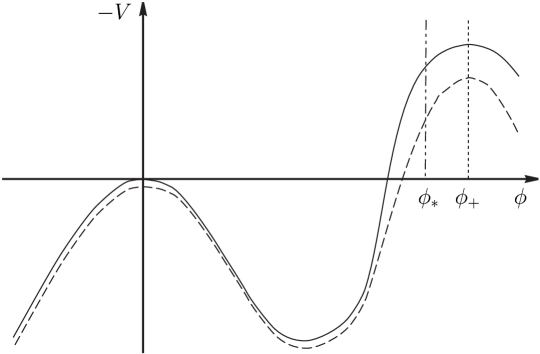
Figure 1: Inverted potential $[-V(\phi)]$ (solid line) and inverted auxiliary potential $[-V_{0}(\phi)]$ (dashed line).

Let $V_{0}(\phi)$ be an auxiliary potential, such that there exists a solution to

$$\frac{d^{2}\phi}{dy^{2}}+4\frac{d\phi}{dy}-\frac{\partial V_{0}}{\partial\phi}=0\;,$$

that starts at $y\to-\infty$ in the true vacuum $\phi=\phi_{+}$ and reaches the false vacuum $\phi=0$ at $y\to\infty$. A necessary condition for the existence of such a sulution is again $V_{0}^{\prime\prime}<-4$ at the maximum of $V_{0}$. Let the potential $V(\phi)$ be a deformation of $V_{0}$ which is deeper than $V_{0}$ in the true vacuum, see Fig. 1. Then, by continuity, there exists a value of $\phi_{*}<\phi_{+}$ such that the solution to eq. (23) starts at $s=0$ from $\phi_{c}=\phi_{*}$ and approaches the false vacuum $\phi=0$ as $s\to\infty$: a solution starting close to the top of $(-V)$ overshoots the false vacuum, while a solution that starts from small $\phi$ undershoots it. This completes the argument.

The bounce solution approaches the false vacuum $\phi=0$ exponentially in $s$,

$$\phi_{c}\to c{\rm e}^{-\Delta_{+}s}\simeq\frac{c}{(2\cosh s)^{\Delta_{+}}}\;,\;\;\;\;\;\;\;c=\mbox{const}\;,\;\;\;s\to\infty\;,$$ (24)

where $\Delta_{+}$ is given by eq. (17) and $m^{2}=V^{\prime\prime}(0)$. We find from eq. (22) that

$$\cosh s=\frac{1+z^{2}+R^{2}}{2z}\equiv\frac{1+z^{2}+x^{2}}{2z}\;.$$ (25)

Hence, $s=\infty$ corresponds to the boundary, and near the boundary

$$\phi_{c}=c\left(\frac{z}{x^{2}+1}\right)^{\Delta_{+}}\;.$$

We compare this with eqs. (16), (18) and find the expectation value of an operator in the (Euclidean) boundary CFT:

$$\langle{\cal O}\rangle=2c\sqrt{m^{2}+4}\cdot\frac{1}{(x^{2}+1)^{\Delta_{+}}}\;.$$ (26)

This is the CFT analog of the Fubini–Lipatov bounce of unit size, cf. eq. (3).

To construct the bounce of arbitrary size, we make yet another change of coordinates,

$${\rm e}^{u}=\sqrt{z^{2}+R^{2}}\;,\;\;\;\;\;\;\cos v=\frac{z}{\sqrt{z^{2}+R^{2}}}\;,$$ (27)

so that

$$\cosh s=\frac{\cosh u}{\cos v}\;,\;\;\;\;\sinh s\cdot\cos\psi=\frac{\sin v}{\cos v}\;.$$ (28)

In terms of these coordinates, the metric is

$$ds_{5}^{2}=\frac{1}{\cos^{2}v}\left(du^{2}+dv^{2}+\sin^{2}vd\Omega_{3}^{2}\right)\;.$$ (29)

Let us write for the bounce of unit size

$$\phi_{c}(s)=f(\cosh s)=f\left(\frac{\cosh u}{\cos v}\right)\;.$$ (30)

Since the metric (29) is invariant under translations of $u$, there is a family of bounce solutions parametrized by a parameter $b$:

$$\phi_{c}^{(b)}=f\left(\frac{\cosh(u+b)}{\cos v}\right)\;$$

(we keep the notation $\phi_{c}$ for the bounce of unit size, i.e., $\phi_{c}\equiv\phi_{c}^{(b=0)}$). The bounce $\phi_{c}^{(b)}$ has size

$$\rho={\rm e}^{-b}\;.$$

One way to see this is to consider the behavior of $\phi_{c}^{(b)}$ near the boundary. Making use of eqs. (24) and (30) we find that $f(C)=c/(2C)^{\Delta_{+}}$ at large $C$, and hence near the boundary

$$\phi_{c}^{(b)}=\frac{c}{\left[2\cosh(u+b)/\cos v\right]^{\Delta_{+}}}\;,$$

which, in view of eq. (27), gives

$$\phi_{c}^{(b)}=cz^{\Delta_{+}}\cdot\frac{{\rm e}^{-\Delta_{+}b}}{\left(R^{2}+{\rm e}^{-2b}\right)^{\Delta_{+}}}=cz^{\Delta_{+}}\left(\frac{\rho}{x^{2}+\rho^{2}}\right)^{\Delta_{+}}\;,\;\;\;\;\;z\to 0\;.$$ (31)

This shows that $\rho$ is indeed the size of the bounce.

Another way to see that $b$ parametrizes the size of the bounce is to consider lines of constant $\phi_{c}^{(b)}$ in the $(z,R)$-plane. Line of constant $\phi_{c}^{(b)}=f(C)$ obeys

$$\frac{\cosh(u+b)}{\cos v}=C\;.$$

For given $C$, these lines are different for different $b$, while the value of $\phi_{c}^{(b)}$ is the same for all $b$. Making use of eq. (27), we find the equation of the line in $(z,R)$-coordinates

$$(z-C{\rm e}^{-b})^{2}+R^{2}=(C^{2}-1){\rm e}^{-2b}\;.$$

It shows that these lines are circles (4-spheres in coordinates $(z,x^{\mu})$) of radii $\sqrt{C^{2}-1}{\rm e}^{-b}$ centered at $z=C{\rm e}^{-b}$, cf. Ref. [22]. As compared to the bounce of unit size ($b=0$), the center of the 5-dimensional bounce (the point where $C=1$) is shifted from $z=1$ to $z={\rm e}^{-b}=\rho$, and the bounce configuration is dilated by a factor ${\rm e}^{-b}=\rho$. This is precisely what one expects for the bounce of size $\rho$ in the holographic picture.

To end up the discussion of the Euclidean bounce, we derive the infinitesimal form of its scale transformation. We write for the transformation of the bounce of unit size

$$\delta_{b}\phi\equiv\frac{\partial\phi_{c}^{(b)}}{\partial b}(b=0)=\frac{df(C)}{dC}~{}\frac{\sinh u}{\cos v}=\frac{d\phi_{c}}{ds}\frac{\sinh u}{\sinh s\cos v}\;.$$

Making use of eq. (28) we obtain finally

$$\delta_{b}\phi=\frac{d\phi_{c}}{ds}\sin\psi\;.$$ (32)

We will use this result in what follows.

3.2 Expanding bubble and its radial perturbations

Without loss of generality, from now on we concentrate on the bounce of unit size. To study the bounce and its perturbations in adS₅ with Minkowski signature, we analytically continue the coordinate $\psi$ in eq. (21),

$$\psi\to i\tau\;,$$

so the metric becomes

$$ds^{2}_{5} =ds^{2}+\sinh^{2}s(-d\tau^{2}+\cosh^{2}\tau d\Omega_{3}^{2})$$

$$=ds^{2}+\sinh^{2}s[-d\tau^{2}+\cosh^{2}\tau(d\chi^{2}+\sin^{2}\chi~{}d\Omega_{2}^{2})]\;.$$ (33)

This is the metric of adS₅ with dS₄ slicing (see, e.g., Ref. [34]): the hypersurfaces $s=\mbox{const}$ are dS₄ spaces with metric proportional to

$$ds_{4}^{2}=-d\tau^{2}+\cosh^{2}\tau d\Omega_{3}^{2}\equiv g_{4\,\mu\nu}dX^{\mu}dX^{\nu}\;.$$ (34)

The region near the adS₅ boundary is conveniently studied using the Poincarè coordinates, in which the metric has the standard form

$$ds_{5}^{2}=\frac{1}{z^{2}}[-(dx^{0})^{2}+dz^{2}+d{\cal R}^{2}+{\cal R}^{2}d\Omega_{2}^{2}]\;,$$

where ${\cal R}$ is the usual radial coordinate in 3d space. The transformation to these coordinates is

$$z =\frac{1}{\cosh s+\sinh s\cosh\tau\cos\chi}$$

$$x^{0} =\frac{\sinh s\sinh\tau}{\cosh s+\sinh s\cosh\tau\cos\chi}$$

$${\cal R} =\frac{\sinh s\cosh\tau\sin\chi}{\cosh s+\sinh s\cosh\tau\cos\chi}\;,$$

or

$$\cosh s=\frac{{\cal R}^{2}-(x^{0})^{2}+z^{2}+1}{2z} \equiv\frac{x^{2}+z^{2}+1}{2z}$$ (36a)

$$\sinh s\sinh\tau=\frac{x^{0}}{z}\;,\;\;\;\;\;\;\;\,\;\;\;\;$$ (36b)

$$\sinh s\cosh\tau\sin\chi=\frac{\cal R}{z}\;,$$ (36c)

where $x^{2}=\eta_{\mu\nu}x^{\mu}x^{\nu}$. The hypersurface $s=0$ is the light cone emanating from $z=1$, $x^{\mu}=0$, so the coordinates used here cover the exterior of this light cone only; since we will be eventually interested in the behavior of the fields near the adS₅ boundary, we will not need to consider the interior of this light cone.

The bounce solution $\phi_{c}(s)$ is the same function of $s$ as before; it obeys eq. (23). Since eq. (36a) formally coincides with eq. (25), the expectation value of the CFT operator is still given by eq. (26), now with Minkowski $x^{2}$. It diverges as $x^{2}\to-1$; in the holographic picture this is the surface at which the light cone $s=0$ hits the adS₅ boundary. According to the general scenario of the (pseudo-)conformal Universe, we assume that the rolling stage terminates before that.

Let us now consider the perturbations about the expanding bubble, $\phi=\phi_{c}(s)+\delta\phi(s,X^{\mu})$, where $X^{\mu}$ are coordinates on dS₄, see eq. (34). We still call $\delta\phi$ radial perturbations. In metric (33) the quadratic action is

$$S_{2}=\int~{}ds~{}d^{4}X~{}\sinh^{4}s\sqrt{-g_{4}}\left[-\frac{1}{2}\left(\partial_{s}\delta\phi\right)^{2}-\frac{1}{2\sinh^{2}s}g^{\mu\nu}_{4}\partial_{\mu}\delta\phi\cdot\partial_{\nu}\delta\phi-\frac{1}{2}V^{\prime\prime}(\phi_{c})\cdot(\delta\phi)^{2}\right]\;,$$

and the field equation reads

$$\partial_{s}^{2}\delta\phi+4\frac{\cosh s}{\sinh s}\delta\phi+\frac{1}{\sinh^{2}s}\Box_{4}\delta\phi-V^{\prime\prime}(\phi_{c})\delta\phi=0\;,$$ (37)

where $\Box_{4}$ is the d’Alembertian in the 4d de Sitter space with metric (34). Solutions to eq. (37) are linear combinations of

$$\delta\phi_{(\mu)}=\Phi_{(\mu)}(s)\Psi_{(\mu)}(X)\;,$$ (38)

where

$$\Box_{4}\Psi_{(\mu)}=\mu^{2}\Psi_{(\mu)}\;,$$ (39)

and $\Phi_{(\mu)}(s)$ obeys the following equation:

$$\frac{d^{2}\Phi_{(\mu)}}{ds^{2}}+4\frac{\cosh s}{\sinh s}\frac{d\Phi_{(\mu)}}{ds}+\frac{\mu^{2}}{\sinh^{2}s}\Phi_{(\mu)}-V^{\prime\prime}(\phi_{c})\Phi_{(\mu)}=0\;.$$ (40)

We will get back to eq. (40) shortly, and now we discuss solutions to eq. (39). The latter is the equation for a field of mass $\mu$ in 4d de Sitter space-time (34). We are again interested in short modes, i.e., modes whose conformal 3d momentum is high, $k\gg 1$. The interesting regime is then $\tau\gg 1$, and the spatial curvature of slices of constant $\tau$ can be neglected. Working near $\chi=0$ without loss of generality, we approximate the metric (34) by the metric of dS₄ with flat slices of constant time,

$$ds_{4}^{2}=-d\tau^{2}+\left(\frac{{\rm e}^{\tau}}{2}\right)^{2}d{\bf x}^{2}=\frac{1}{\eta^{2}}(-d\eta^{2}+d{\bf x}^{2})\;,$$

where

$$\eta=-2{\rm e}^{-\tau}\;.$$ (41)

Upon introducing the field $\sigma_{(\mu)}=\Psi_{(\mu)}/\eta$, the field equation (39) becomes

$$-\partial_{\eta}^{2}\sigma_{(\mu)}+\Delta\sigma_{(\mu)}+\frac{2-\mu^{2}}{\eta^{2}}\sigma_{(\mu)}=0\;,$$

where $\Delta$ is the flat 3d Laplacian. In 3d momentum representation its solutions tending to $e^{-ik\eta}/\sqrt{2k}$ as $\eta\to-\infty$ are

$$\sigma_{(\mu)}=\frac{\sqrt{\pi|\eta|}}{2}H_{\nu}^{(1)}(-k\eta)\;,$$

where

$$\nu=\sqrt{\frac{9}{4}-\mu^{2}}\;.$$

For real $\nu$ the asymptotics of these solutions as $k|\eta|\to 0$ are

$$\sigma_{(\mu)}=-i\frac{\sqrt{\pi}2^{\nu-1}}{\Gamma(1-\nu)\sin{\nu\pi}}\frac{1}{k^{\nu}(-\eta)^{\nu-1/2}}\;,$$

and the late-time asymptotics of $\Psi_{(\mu)}$ are

$$\Psi_{(\mu)}=-i\frac{\sqrt{\pi}2^{\nu-1}}{\Gamma(1-\nu)\sin{\nu\pi}}\frac{1}{k^{\nu}(-\eta)^{\nu-3/2}}\;,\;\;\;\;\;\;\;\;k|\eta|\ll 1\;.$$ (42)

For $\nu>1/2$ the modes $\sigma_{(\mu)}$ are enhanced at $k|\eta|\ll 1$ as compared to massless Minkowski theory, in which $g\propto k^{-1/2}$. In what follows we consider the case

$$\mu^{2}<2\;,\;\;\;\;\;\;\;\nu>1/2\;.$$

In this case the quantum field associated with the mode of mass $\mu$ can be considered as classical random field [35] with power spectrum ${\cal P}_{(\mu)}\propto k^{-2\nu+3}$.

Let us now turn to eq. (40). For $\mu^{2}<2$ this is an eigenvalue equation for $\mu^{2}$. We normalize its solutions as follows:

$$\int~{}ds~{}\sinh^{2}s~{}|\Phi_{(\mu)}|^{2}=1\;,$$ (43)

then the field $\Psi_{(\mu)}(X)$ has canonical kinetic term. The eigenfunctions must behave at large $s$ (near the adS₅ boundary) as follows,

$$\Phi_{(\mu)}=C_{(\mu)}{\rm e}^{-\Delta_{+}s}$$ (44)

(another asymptotic behavior $\Phi_{(\mu)}\propto{\rm e}^{-\Delta_{-}s}$ with $\Delta_{-}=2-\sqrt{4+m^{2}}$ would correspond to a non-zero source at the boundary), where $C_{(\mu)}$ is determined by the normalization condition (43). Near $s=0$ the solutions are $\Phi_{(\mu)}\propto s^{n_{\pm}}$, where $n_{\pm}=-\frac{3}{2}\pm\sqrt{\frac{9}{4}-\mu^{2}}$. For $\mu^{2}<2$ one of them is normalizable, and another is not. Hence, we are indeed dealing with an eigenvalue problem.

Let us consider the behavior of the modes near the boundary $s\to\infty$ and at late times. We are interested in short modes and, as before, work in the vicinity of $\chi=0$. Making use of eq. (36a) we translate eq. (44) into

$$\Phi_{(\mu)}=C_{(\mu)}\frac{z^{\Delta_{+}}}{(x^{2}+1)^{\Delta_{+}}}\;,\;\;\;\;\;\;z\to 0\;.$$

We recall eqs. (41) and (36b) to write at large $s$

$$-\eta=\frac{x^{2}+1}{2x^{0}}\;.$$

Furthermore, our region of small $\chi$ and $x^{2}\to-1$ corresponds to $x^{0}\to 1$, ${\cal R}\ll x^{0}$, see eqs. (36b) and (36c). We use eq. (42) and get finally

$$\delta\phi_{(\mu)}=-iC_{(\mu)}\frac{\sqrt{\pi}2^{2\nu-5/2}}{\Gamma(1-\nu)\sin{\nu\pi}}\cdot\frac{z^{\Delta_{+}}}{(x^{2}+1)^{\Delta_{+}+\nu-3/2}}\cdot\frac{1}{k^{\nu}}\cdot B_{\bf k}+\mbox{h.~{}c.}\;,\;\;\;\;\;\;z\to 0\;,~{}k(x^{2}+1)\ll 1\;,$$

where $B_{\bf k}$ is annihilation operator. The radial perturbations in the boundary CFT are obtained from eqs. (17), (18):

$$\delta{\cal O}_{(\mu)}=-iC_{(\mu)}\sqrt{m^{2}+4}\frac{\sqrt{\pi}2^{2\nu-3/2}}{\Gamma(1-\nu)\sin{\nu\pi}}\cdot\frac{1}{(x^{2}+1)^{\Delta_{+}+\nu-3/2}\cdot k^{\nu}}\cdot B_{\bf k}+\mbox{h.~{}c.}\;,\;\;z\to 0\;,~{}k(x^{2}+1)\ll 1\;.$$ (45)

For $\nu>1/2$ these modes have enhanced power spectrum, so they may lead to interesting effects beyond the linear level.

Now, the key point out that eq. (40) always admits a solution with

$$\mu^{2}=-4\;.$$

This solution is

$$\Phi_{(\mu^{2}=-4)}=\frac{d\phi_{c}}{ds}\;.$$ (46)

One can view its existence as a consequence of the dilatational invariance. Indeed, this invariance guarantees that the function (32) is a solution to the equation for perturbations in the Euclidean domain, its counterpart in Minkowski signature being

$$\delta_{b}\phi=\frac{d\phi_{c}}{ds}\sinh\tau\;.$$

This solution has the form (38), and the 4d factor $\sinh\tau$ obeys eq. (39) with $\mu^{2}=-4$. Hence, $d\phi_{c}/ds$ must obey eq. (40) with $\mu^{2}=-4$, and it indeed does. Note that the solution (46) does not have nodes, which implies that $\mu^{2}=-4$ is the lowest eigenvalue of eq. (40). Therefore, the leading asymptotics of $\delta{\cal O}$ at late times ($x^{2}\to-1$) is determined by the mode with $\mu^{2}=-4$.

For $\mu^{2}=-4$ we have $\nu=5/2$, and the late-time asymptotics of the CFT operator (45) reads

$$\delta{\cal O}_{(\mu^{2}=-4)}=-iC_{(\mu^{2}=-4)}\sqrt{m^{2}+4}\cdot 3\cdot 2^{3/2}\cdot\frac{1}{(x^{2}+1)^{\Delta_{+}+1}\cdot k^{5/2}}\cdot B_{\bf k}+\mbox{h.~{}c.}\;.$$ (47)

In complete analogy to eq. (10), these radial perturbations in the boundary CFT have red power spectrum ${\cal P}_{\delta{\cal O}}\propto k^{-2}$. In view of eq. (31) and by the same argument as in Section 2.2, the dependence on $x$ in (47) can be interpreted as the effect of spatially varying scale $\rho({\bf x})$. This is the desired result.

3.3 Dimension-zero field: phase

Let us extend the model by promoting the field $\phi$ to a complex scalar field. With the kinetic term $(1/2)\partial\phi^{*}\partial\phi$ and $V=V(|\phi|)$, the model has now a global $U(1)$ symmetry. We take the bounce/bubble solution $\phi_{c}$ real, then away from $\phi=0$, the phase $\mbox{Arg}~{}\phi$ corresponds to a dimension-zero operator, the phase of ${\cal O}$. To study its late-time perturbations, we consider the field $\varphi=\mbox{Im}~{}\phi$. The quadratic action is

$$S_{2}=\int~{}ds~{}d^{4}X~{}\sinh^{4}s\sqrt{-g_{4}}\left[-\frac{1}{2}\left(\partial_{s}\varphi\right)^{2}-\frac{1}{2\sinh^{2}s}g^{\mu\nu}_{4}\partial_{\mu}\varphi\partial_{\nu}\varphi-\frac{1}{2}\frac{V^{\prime}(\phi_{c})}{\phi_{c}}\varphi^{2}\right]\;.$$

The solutions to the field equation again have the product form (38) where the 4d part obeys eq. (39), while the equation for the $s$-dependent factor, which we denote by $\Phi_{I,(\mu)}$, is

$$\partial_{s}^{2}\Phi_{I,(\mu)}+4\frac{\cosh s}{\sinh s}\Phi_{I,(\mu)}+\frac{\mu^{2}}{\sinh^{2}s}\Phi_{I,(\mu)}-\frac{V^{\prime}(\phi_{c})}{\phi_{c}}\Phi_{I,(\mu)}=0\;.$$ (48)

It has a solution with $\mu=0$; this is $\Phi_{I,(\mu=0)}=\phi_{c}$. The existence of this mode is guaranteed by the $U(1)$-symmetry: both $\phi_{c}$ and ${\rm e}^{i\alpha}\phi_{c}$ are solutions to the full non-linear field equation, so $i\alpha\phi_{c}$ must be a solution for the linearized equation for perturbations for $k=0$. The solution $\Phi_{I,(\mu=0)}=\phi_{c}$ again does not have nodes, so it is the lowest eigenmode of eq. (48) which determines the leading late-time asymptotics of $\mbox{Im}~{}{\cal O}$.

For $\mu^{2}=0$ we have $\nu=3/2$, and eq. (45) gives

$$\mbox{Im}~{}{\cal O}=-iC_{(\mu=0)}\sqrt{2(m^{2}+4)}\cdot\frac{1}{(x^{2}+1)^{\Delta_{+}}\cdot k^{3/2}}\cdot A_{\bf k}+\mbox{h.~{}c.}\;,\;\;z\to 0\;,~{}k(x^{2}+1)\ll 1\;,$$

where $A_{\bf k}$ is another annihilation operator. Thus, the phase $\Theta=\mbox{Im}~{}{\cal O}/\langle{\cal O}\rangle$ freezes out at late times at

$$\Theta=-i\frac{C_{(\mu=0)}}{\sqrt{2}c}\cdot\frac{1}{k^{3/2}}\cdot A_{\bf k}+\mbox{h.~{}c.}\;,$$

where the constant $c$ is determined by the bounce solution via eq. (24). In complete analogy to Section 2.3, the phase perturbations have flat power spectrum

$${\cal P}_{\Theta}=\frac{1}{4\pi^{2}}\left(\frac{C_{(\mu=0)}}{c}\right)^{2}\;.$$

We conclude that our holographic model shares all late-time properties of the 4d
(pseudo-)conformal models.

4 Conclusion

While the overall picture of the (pseudo-)conformal Universe is the same in the false vacuum decay and original homogeneous rolling models, the former may have peculiarities. First, the slices on which the background is homogeneous, are not spatially flat. Depending on the embedding of the (pseudo-)conformal mechanism into a complete cosmological scenario, this may or may not give rise to novel properties of the resulting adiabatic perturbations, such as particular form of statistical anisotropy. Second, in the holographic model there may exist modes, which are subdominant at late times (with $\mu^{2}>-4$ and $\mu^{2}>0$ for radial and phase perturbations, respectively), but nevertheless relevant. Also, back reaction of the bounce and its perturbations on space-time metric, which we neglected in this paper, may possibly lead to interesting effects. We leave the analysis of these and other issues for future work.

We are indebted to R. Gopakumar, R. Rattazzi, S. Sibiryakov and A. Starinets for useful discussions. The work of M.L. and V.R. has been supported by Russian Science Foundation grant 14-22-00161.

References

- [1] V. A. Rubakov, JCAP 0909 (2009) 030 [arXiv:0906.3693 [hep-th]].
- [2] P. Creminelli, A. Nicolis and E. Trincherini, JCAP 1011 (2010) 021 [arXiv:1007.0027 [hep-th]].
- [3] K. Hinterbichler and J. Khoury, JCAP 1204 (2012) 023 [arXiv:1106.1428 [hep-th]].
- [4] K. Hinterbichler, A. Joyce, J. Khoury and G. E. J. Miller, JCAP 1212 (2012) 030 [arXiv:1209.5742 [hep-th]].
- [5] I. Antoniadis, P. O. Mazur and E. Mottola, Phys. Rev. Lett. 79 (1997) 14 [arXiv:astro-ph/9611208].
- [6] M. Osipov and V. Rubakov, JETP Lett. 93 (2011) 52 [arXiv:1007.3417 [hep-th]].
- [7] Y. Wang and R. Brandenberger, JCAP 1210 (2012) 021 [arXiv:1206.4309 [hep-th]].
-
[8]
A. D. Linde and V. F. Mukhanov,
Phys. Rev. D 56 (1997), 535
[astro-ph/9610219];
K. Enqvist and M. S. Sloth, Nucl. Phys. B 626 (2002), 395 [hep-ph/0109214];
D. H. Lyth and D. Wands, Phys. Lett. B 524 (2002), 5 [hep-ph/0110002];
T. Moroi and T. Takahashi, Phys. Lett. B 522 (2001), 215 [Erratum-ibid. B 539 (2002), 303] [hep-ph/0110096];
K. Dimopoulos, D. H. Lyth, A. Notari and A. Riotto, JHEP 0307, (2003), 053 [hep-ph/0304050]. -
[9]
G. Dvali, A. Gruzinov and M. Zaldarriaga,
Phys. Rev. D 69 (2004), 023505
[astro-ph/0303591];
L. Kofman, Probing string theory with modulated cosmological fluctuations, astro-ph/0303614;
G. Dvali, A. Gruzinov and M. Zaldarriaga, Phys. Rev. D 69 (2004), 083505 [astro-ph/0305548]. -
[10]
J. Khoury, P. J. Steinhardt and N. Turok,
Phys. Rev. Lett. 92, 031302 (2004)
[hep-th/0307132];
E. I. Buchbinder, J. Khoury and B. A. Ovrut, Phys. Rev. D 76, 123503 (2007) [hep-th/0702154]; JHEP 0711, 076 (2007) [arXiv:0706.3903 [hep-th]];
P. Creminelli and L. Senatore, JCAP 0711, 010 (2007) [hep-th/0702165];
Y. -F. Cai, D. A. Easson and R. Brandenberger, JCAP 1208, 020 (2012) [arXiv:1206.2382 [hep-th]];
M. Gasperini and G. Veneziano, Phys. Rept. 373, 1 (2003) [hep-th/0207130];
J. K. Erickson, D. H. Wesley, P. J. Steinhardt and N. Turok, Phys. Rev. D 69, 063514 (2004) [hep-th/0312009];
T. Qiu, J. Evslin, Y. -F. Cai, M. Li and X. Zhang, JCAP 1110, 036 (2011) [arXiv:1108.0593 [hep-th]];
D. A. Easson, I. Sawicki and A. Vikman, JCAP 1111, 021 (2011) [arXiv:1109.1047 [hep-th]];
M. Osipov and V. Rubakov, JCAP 1311 (2013) 031 [arXiv:1303.1221 [hep-th]]. - [11] P. Creminelli, M. A. Luty, A. Nicolis and L. Senatore, JHEP 0612, 080 (2006) [hep-th/0606090].
- [12] P. Creminelli, K. Hinterbichler, J. Khoury, A. Nicolis and E. Trincherini, JHEP 1302 (2013) 006 [arXiv:1209.3768 [hep-th]].
- [13] M. Libanov, S. Ramazanov and V. Rubakov, JCAP 1106 (2011) 010 [arXiv:1102.1390 [hep-th]].
-
[14]
M. Libanov and V. Rubakov,
JCAP 1011 (2010) 045
[arXiv:1007.4949 [hep-th]];
M. V. Libanov and V. A. Rubakov, Theor. Math. Phys. 170 (2012) 151 [Teor. Mat. Fiz. 170 (2012) 188]. - [15] P. Creminelli, A. Joyce, J. Khoury and M. Simonovic, JCAP 1304 (2013) 020 [arXiv:1212.3329].
- [16] S. R. Ramazanov and G. I. Rubtsov, JCAP 1205 (2012) 033 [arXiv:1202.4357 [astro-ph.CO]]; Phys. Rev. D 89 (2014) 043517 [arXiv:1311.3272 [astro-ph.CO]]; Phys. Rev. D 91 (2015) 4, 043514 [arXiv:1406.7722 [astro-ph.CO]].
-
[17]
M. Libanov, S. Mironov and V. Rubakov,
Phys. Rev. D 84 (2011) 083502
[arXiv:1105.6230 [astro-ph.CO]];
M. Libanov, S. Mironov and V. Rubakov, Prog. Theor. Phys. Suppl. 190 (2011) 120;
S. A. Mironov, S. R. Ramazanov and V. A. Rubakov, JCAP 1404 (2014) 015 [arXiv:1312.7808 [astro-ph.CO]]. - [18] K. Hinterbichler, A. Joyce and J. Khoury, JCAP 1206 (2012) 043 [arXiv:1202.6056 [hep-th]].
- [19] S. Fubini, Nuovo Cim. A 34 (1976) 521.
- [20] L. N. Lipatov, Sov. Phys. JETP 45 (1977) 216 [Zh. Eksp. Teor. Fiz. 72 (1977) 411].
- [21] J. M. Maldacena, J. Michelson and A. Strominger, JHEP 9902 (1999) 011 [hep-th/9812073].
- [22] A. S. Gorsky and K. G. Selivanov, Int. J. Mod. Phys. 16 (2001) 2243 [hep-th/0006044].
- [23] T. Hertog and G. T. Horowitz, JHEP 0407 (2004) 073 [hep-th/0406134]; JHEP 0504 (2005) 005 [hep-th/0503071].
- [24] B. Craps, T. Hertog and N. Turok, Phys. Rev. D 80 (2009) 086007 [arXiv:0905.0709 [hep-th]]; Phys. Rev. D 86 (2012) 043513 [arXiv:0712.4180 [hep-th]].
- [25] J. L. F. Barbon and E. Rabinovici, JHEP 1004 (2010) 123 [arXiv:1003.4966 [hep-th]]; JHEP 1104 (2011) 044 [arXiv:1102.3015 [hep-th]].
- [26] D. Harlow, “Metastability in Anti de Sitter Space,” arXiv:1003.5909 [hep-th].
- [27] K. Hinterbichler, J. Stokes and M. Trodden, “Holography for a Non-Inflationary Early Universe,” arXiv:1408.1955 [hep-th].
- [28] M. Libanov, V. Rubakov and S. Sibiryakov, Phys. Lett. B 741 (2015) 239 [arXiv:1409.4363 [hep-th]].
- [29] J. Distler and F. Zamora, Adv. Theor. Math. Phys. 2 (1999) 1405 [hep-th/9810206].
- [30] R. Sundrum, Phys. Rev. D 86, 085025 (2012) [arXiv:1106.4501 [hep-th]].
- [31] V. Balasubramanian, P. Kraus, A. E. Lawrence and S. P. Trivedi, Phys. Rev. D 59 (1999) 104021 [hep-th/9808017].
- [32] I. R. Klebanov and E. Witten, Nucl. Phys. B 556 (1999) 89 [hep-th/9905104].
- [33] V. A. Rubakov and S. M. Sibiryakov, Theor. Math. Phys. 120, 1194 (1999) [Teor. Mat. Fiz. 120, 451 (1999)] [gr-qc/9905093].
- [34] G. Goon, K. Hinterbichler and M. Trodden, JCAP 1107 (2011) 017 [arXiv:1103.5745 [hep-th]].
-
[35]
D. Polarski and A. A. Starobinsky,
Class. Quant. Grav. 13 (1996) 377
[gr-qc/9504030];
C. Kiefer, D. Polarski and A. A. Starobinsky, Int. J. Mod. Phys. D 7 (1998) 455 [gr-qc/9802003].