Spectral-Domain Computation of Fields Radiated by Sources in Non-Birefringent Anisotropic Media

Abstract

We derive the key expressions to robustly address the eigenfunction expansion-based analysis of electromagnetic (EM) fields produced by current sources within planar non-birefringent anisotropic medium (NBAM) layers. In NBAM, the highly symmetric permeability and permittivity tensors can induce directionally-dependent, but polarization independent, propagation properties supporting “degenerate” characteristic polarizations, i.e. four linearly-independent eigenvectors associated with only two (rather than four) unique, non-defective eigenvalues. We first explain problems that can arise when the source(s) specifically reside within NBAM planar layers when using canonical field expressions. To remedy these problems, we exhibit alternative spectral-domain field expressions, immune to such problems, that form the foundation for a robust eigenfunction expansion-based analysis of time-harmonic EM radiation and scattering within such type of planar-layered media. Numerical results demonstrate the high accuracy and stability achievable using this algorithm.

I Introduction

Environments with (locally) planar-layered profiles are encountered in diverse applications such as geophysical exploration, ground penetrating radar, conformal antenna design, and so on [1, 2, 3]. To facilitate electromagnetic (EM) radiation analysis in such environments, eigenfunction (plane wave) expansions (PWE) have long been used because of their relative computational efficiency versus brute-force numerical methods such as finite difference and finite element methods. Moreover, PWE can accommodate linear, but otherwise arbitrary anisotropic layers characterized by arbitrary (diagonalizable) 3$\times$3 material tensors [1]. This proves useful when rigorously modeling planar media simultaneously exhibiting both electrical and magnetic anisotropy, such as (i) isoimpedance beam-shifting devices and (to facilitate proximal antenna placement) ground-plane-coating slabs systematically designed via transformation optics (T.O.) techniques [2, 4], (ii) more practically realizable (albeit not necessarily isoimpedance) approximations to T.O.-inspired media such as metamaterial-based thin, wide-angle, and polarization-robust absorbers to facilitate (for example) radar cross section control [5], as well as (iii) numerous other media such as certain types of liquid crystals, elastic media subject to small deformations, and superconductors at high temperatures [6]. These named, amongst other, modeling scenarios share in common the potential presence of a particular class of anisotropic media in which the magnetic permeability ($\bm{\bar{\mu}}_{r}$) and electric permittivity ($\bm{\bar{\epsilon}}_{r}$) tensor properties are “matched” to each other and hence together define media supporting four “degenerate” plane wave eigenfunctions that, while possessing four linearly independent field polarization states (eigenvectors) as usual, share only two unique (albeit, critically still, non-defective) eigenvalues [7]. Alternatively stated, propagation characteristics within such media are still (in general) dependent on propagation direction but independent of polarization, eliminating “double refraction” (“birefringence”) effects [7, 6]. Hence our proposed moniker “Non-Birefringent Anisotropic Medium” (NBAM), rather than the “pseudo-isotropic” moniker [6].

From an analytical standpoint, said PWE constitute spectral integrals exactly quantifying the radiated fields [2]. Except for some very simple cases however, these expansions must almost always be evaluated by means of numerical quadratures or cubatures, whose robust computation (with respect to varying source and layer properties) is far from trivial and requires careful choice of appropriate quadrature rules, complex-plane integration contours, etc. to mitigate discretization and truncation errors as well as accelerate convergence [1, 2, 8]. In addition to such considerations of primarily numerical character, a distinct problem occurs, due to said eigenvalue degeneracy, when sources radiate within NBAM layers. Indeed, this case requires proper analytical “pre-treatment” of the fundamental spectral-domain field expressions to avoid two sources of “breakdown”: (i) Numerically unstable calculations (namely, divisions by zero) during the computation chain, as well as (ii) Corruption of the correct form of the eigenfunctions, viz. $z$exp[$ik_{z}z$] instead of the proper form exp[$ik_{z}z$], the former resulting from a naive, “blanket” application of Cauchy’s integral theorem to the canonical field expressions [9, 10].

To this end, we first show the key results detailing the degenerate “direct” (i.e., homogeneous medium) radiated fields in the “principal material basis” (PMB) representation with respect to which the material tensors are assumed simultaneously diagonalized by an orthogonal basis [4]. Subsequently, we transform these PMB expressions to the Cartesian basis (the PWE’s employed basis). Finally, we employ a robust, numerically-stable NBAM polarization decomposition scheme to obtain the Cartesian-basis direct field polarization amplitudes. The two-dimensional (2-D) Fourier integral-based PWE algorithm, resulting from implanting these derived field expressions into an otherwise highly robust PWE algorithm [2], comprises this paper’s central contribution.

II Problem Statement

We assume the $\exp{-i\omega t}$ convention in what follows. Within a homogeneous medium of material properties $\{\bm{\bar{\epsilon}}_{r},\bm{\bar{\mu}}_{r}\}$, the electric field $\bm{\mathcal{E}}(\mathbb{r})$ radiated by electric ($\bm{\mathcal{J}}$) and (equivalent) magnetic ($\bm{\mathcal{M}}$) current sources satisfies

$$\bm{\mathcal{\bar{A}}}(\cdot)=\nabla\times\bm{\bar{\mu}}^{-1}_{r}\cdot\nabla\times(\cdot)-k_{0}^{2}\bm{\bar{\epsilon}}_{r}\cdot(\cdot)$$ (II.1)

$$\bm{\mathcal{\bar{A}}}(\bm{\mathcal{E}})=ik_{o}\eta_{o}\bm{\mathcal{J}}-\nabla\times\bm{\bar{\mu}}^{-1}_{r}\cdot\bm{\mathcal{M}}$$ (II.2)

and can be expressed via a 3-D Fourier integral over the field’s plane wave constituents $\{\mathbb{\tilde{E}}(\mathbb{k})\mathrm{e}^{i\mathbb{k}\cdot\mathbb{r}}\}$:

$$\mathbb{\tilde{\bar{A}}}^{-1} =\mathrm{Adj}\left(\mathbb{\tilde{\bar{A}}}\right)/\mathrm{Det}\left(\mathbb{\tilde{\bar{A}}}\right)$$ (II.3)

$$\mathbb{\tilde{E}}(\mathbb{k}) =\mathbb{\tilde{\bar{A}}}^{-1}\cdot\left[ik_{0}\eta_{0}\mathbb{\tilde{J}}-\tilde{\nabla}\times\bm{\bar{\mu}}^{-1}_{r}\cdot\mathbb{\tilde{M}}\right]$$ (II.4)

$$\bm{\mathcal{E}}(\mathbb{r}) =\left(\frac{1}{2\pi}\right)^{3}\iiint\limits_{-\infty}^{+\infty}\mathbb{\tilde{E}}(\mathbb{k})\,\mathrm{e}^{i\mathbb{k}\cdot\mathbb{r}}\,\mathrm{d}k_{z}\,\mathrm{d}k_{x}\,\mathrm{d}k_{y}$$ (II.5)

where, anticipating planar layering along $z$, the $k_{z}$ spectral integral is “analytically” evaluated for every ($k_{x},k_{y}$) doublet manifest in the (typically numerically) evaluated outer 2-D Fourier integral. That is to say, by “analytically” evaluated we mean that the general (symbolic) closed-form solution of the $k_{z}$ integral for arbitrary $(k_{x},k_{y})$ doublet, obtained by equivalently viewing the $k_{z}$ real-axis integral as a contour integral evaluated using Jordan’s Lemma and residue calculus, is well-known and can be numerically evaluated at the $(k_{x},k_{y})$ doublets [1, 11]. In particular, analytical evaluation of the $k_{z}$ integral yields the “direct” field $\bm{\mathcal{E}}^{d}(\mathbb{r})$ [1]:

$$\bm{\mathcal{E}}^{d}(\mathbb{r})=\frac{i}{(2\pi)^{2}}\iint\limits_{-\infty}^{+\infty}\Bigg{[}u(\Delta z)\sum_{n=1}^{2}{\tilde{a}_{n}^{d}\mathbb{\tilde{e}}_{n}\mathrm{e}^{i\tilde{k}_{nz}\Delta z}}+\\ u(-\Delta z)\sum_{n=3}^{4}{\tilde{a}_{n}^{d}\mathbb{\tilde{e}}_{n}\mathrm{e}^{i\tilde{k}_{nz}\Delta z}}\Bigg{]}\mathrm{e}^{ik_{x}\Delta x+ik_{y}\Delta y}\,\mathrm{d}k_{x}\,\mathrm{d}k_{y}$$ (II.6)

where $\tilde{a}_{n}^{d}(k_{x},k_{y})$ is the (source dependent) direct field amplitude of the $n$th polarization, while $\mathbb{\tilde{e}}_{n}(k_{x},k_{y})$ and $\tilde{k}_{nz}(k_{x},k_{y})$ are (resp.) the electric field eigenvector (i.e., polarization state) and eigenvalue of the $n$th mode ($n=1,2,3,4$) [1]. Modes labeled with $n=1,2$ correspond to up-going polarizations, and similarly for down-going modes ($n=3,4$).

The problem with the canonical numerical implementation of this residue calculus approach lies in its tacit assumption of non-degeneracy (distinctness) in the eigenvalues $\{\tilde{k}_{1z},\tilde{k}_{2z},\tilde{k}_{3z},\tilde{k}_{4z}\}$, which does not hold for NBAM media. As an illustration of the polarization-independent dispersion behavior of NBAM, consider the dispersion relations of a uniaxial-anisotropic medium slab $\{\bm{\bar{\epsilon}}_{r}=\mathrm{Diag}\left[a,a,b\right],\bm{\bar{\mu}}_{r}=\mathrm{Diag}\left[c,c,d\right]\}$ ($k_{\rho}^{2}=k_{x}^{2}+k_{y}^{2}$) [7, 11]: $\tilde{k}_{1z}=\left[k^{2}_{0}ac-(c/d)k_{\rho}^{2}\right]^{1/2}$, $\tilde{k}_{2z}=\left[k^{2}_{0}ac-(a/b)k_{\rho}^{2}\right]^{1/2}$, $\tilde{k}_{3z}=-\tilde{k}_{1z}$, and $\tilde{k}_{4z}=-\tilde{k}_{2z}$. Setting $\{a=\bar{y}^{2}c,b=\bar{y}^{2}d\}$ ($\bar{y}$ is an arbitrary, non-zero multiplicative constant) renders $\tilde{k}_{z}^{+}=\tilde{k}_{1z}=\tilde{k}_{2z}$ and $\tilde{k}_{z}^{-}=\tilde{k}_{3z}=\tilde{k}_{4z}$, demonstrating the plane wave propagation direction dependent, but polarization independent, dispersion characteristics of uniaxial NBAM [6]. This conclusion applies also for more general uniaxial NBAM material tensors possessing PMB rotated with respect to the Cartesian basis [6]. Similarly, for biaxial NBAM with PMB-expressed tensors $\{\bm{\bar{\mu}}_{r}^{\mathrm{pmb}}=\mathrm{Diag}\left[a,b,c\right],\bm{\bar{\epsilon}}_{r}^{\mathrm{pmb}}=\bar{y}^{2}\bm{\bar{\mu}}_{r}^{\mathrm{pmb}}\}$, the polarization-independent dispersion relations are:

$$\tilde{k}_{1z}^{\mathrm{pmb}} =\left[(\bar{y}k_{0})^{2}ab-(a/c)k_{x}^{2}-(b/c)k_{y}^{2}\right]^{1/2}$$ (II.7)

$$\tilde{k}_{3z}^{\mathrm{pmb}} =-\left[(\bar{y}k_{0})^{2}ab-(a/c)k_{x}^{2}-(b/c)k_{y}^{2}\right]^{1/2}$$ (II.8)

with $\tilde{k}_{z}^{+}=\tilde{k}_{2z}^{\mathrm{pmb}}=\tilde{k}_{1z}^{\mathrm{pmb}}$ and $\tilde{k}_{z}^{-}=\tilde{k}_{4z}^{\mathrm{pmb}}=\tilde{k}_{3z}^{\mathrm{pmb}}$.

Now, the two-fold degenerate eigenvalue $\tilde{k}_{z}^{+}$ has associated with it two linearly independent field polarizations describing up-going plane waves [6]; this holds likewise for the two down-going polarizations with common eigenvalue $\tilde{k}_{z}^{-}$. Mathematically speaking, the eigenvalues $\{\tilde{k}_{z}^{+},\tilde{k}_{z}^{-}\}$ are each twice-repeating (i.e., algebraic multiplicity of two) but have associated with each of them two linearly independent eigenvectors (i.e., geometric multiplicity of two), making them non-defective and rendering the four NBAM polarization states suitable as a local EM field basis within NBAM layers [9]. Despite the existence of four linearly independent eigenvectors, it is worthwhile to further exhibit the key results of the systematic analytical treatment of the two fictitious double-poles of $\mathbb{\tilde{\bar{A}}}^{-1}$ to render numerical PWE-based EM field evaluation robust to the two said sources of “breakdown”; this treatment is performed in the next section.

Let us first make two preliminary remarks, however. First, assume that the source-containing layer is a biaxial NBAM with $\bm{\bar{\mu}}_{r}^{\mathrm{pmb}}=\mathrm{Diag}\left[a,b,c\right]$ and $\bm{\bar{\epsilon}}_{r}^{\mathrm{pmb}}=\bar{y}^{2}\bm{\bar{\mu}}_{r}^{\mathrm{pmb}}$. Second, the orthogonal matrix $\mathbb{\bar{U}}=\begin{bmatrix}\mathbb{\hat{v}}_{1}&\mathbb{\hat{v}}_{2}&\mathbb{\hat{v}}_{3}\end{bmatrix}$ transforms vectors between the PMB and Cartesian basis. For example, the relationship between the $n$th PMB eigenmode wave vector $\mathbb{k}^{\mathrm{pmb}}_{n}=(k_{nx}^{\mathrm{pmb}},k_{ny}^{\mathrm{pmb}},\tilde{k}_{nz}^{\mathrm{pmb}})$ and the (assumed available) $n$th Cartesian-basis wave vector $\mathbb{k}_{n}=(k_{x},k_{y},\tilde{k}_{nz})$ writes as $\mathbb{k}^{\mathrm{pmb}}_{n}=\mathbb{\bar{U}}^{-1}\cdot\mathbb{k}_{n}$.

III Direct Electric Field Radiated within NBAM

The (Cartesian basis) Fourier domain representation of the electric field, radiated in a homogeneous NBAM, writes as $\mathbb{\tilde{E}}=-\mathbb{\tilde{\bar{A}}}^{-1}\cdot\mathbb{\tilde{\nabla}}\times\bm{\bar{\mu}}^{-1}_{r}\cdot\mathbb{\tilde{M}}$ for a (equivalent) magnetic current source or $\mathbb{\tilde{E}}=ik_{0}\eta_{0}\mathbb{\tilde{\bar{A}}}^{-1}\cdot\mathbb{\tilde{J}}$ for an electric current source. These two equations, moreover, hold equally when re-represented in the NBAM’s PMB (i.e., adding “pmb” superscript to all quantities), which is what we will employ. Indeed, the components $\{A_{mw}\}$ ($m,w=1,2,3$) of $\mathbb{\tilde{\bar{A}}}^{-1,\mathrm{pmb}}(\cdot)$ write as ($A_{mw}=A_{wm}$, and $\mathbb{\bar{k}}=\mathbb{k}^{\mathrm{pmb}}/k_{0}$):

$$\tilde{B} =-c\bar{y}^{2}k_{0}^{2}\left(\bar{k}_{z}^{2}-\left[ab\bar{y}^{2}-(a/c)\bar{k}_{x}^{2}-(b/c)\bar{k}_{y}^{2}\right]\right)$$ (III.1)

$$A_{11} =\left(\bar{k}_{x}^{2}-bc\bar{y}^{2}\right)/\tilde{B},\ A_{12}=\bar{k}_{x}\bar{k}_{y}/\tilde{B}$$ (III.2)

$$A_{13} =\bar{k}_{x}\bar{k}_{z}/\tilde{B},\ A_{22}=\left(\bar{k}_{y}^{2}-ac\bar{y}^{2}\right)/\tilde{B}$$ (III.3)

$$A_{23} =\bar{k}_{y}\bar{k}_{z}/\tilde{B},\ A_{33}=\left(\bar{k}_{z}^{2}-ab\bar{y}^{2}\right)/\tilde{B}$$ (III.4)

while the components of $-\mathbb{\tilde{\bar{A}}}^{-1,\mathrm{pmb}}\cdot\mathbb{\tilde{\nabla}}^{\mathrm{pmb}}\times\bm{\bar{\mu}}^{-1,\mathrm{pmb}}_{r}(\cdot)$ $\{\dot{A}_{mw}\}$ write as ($\dot{A}_{mw}=-\dot{A}_{wm}$):

$$\tilde{B}^{\prime} =\tilde{B}/(\bar{y}^{2}),\ \dot{A}_{12}=-ick_{z}/\tilde{B}^{\prime}$$ (III.5)

$$\dot{A}_{13} =ibk_{y}/\tilde{B}^{\prime},\ \dot{A}_{23}=-iak_{x}/\tilde{B}^{\prime}$$ (III.6)

The expressions within Eqns. (III.1)-(III.4) describe the electric field from an electric current source while the expressions within Eqns. (III.5)-(III.6) describe the electric field from an (equivalent) magnetic current source. Duality in Maxwell’s Equations makes immediate the magnetic field results.

Next the PMB electric field $\mathbb{E}^{\mathrm{pmb}}(k_{x},k_{y};z,z^{\prime})$, after re-expressing Eqns. (III.1)-(III.6) in terms of $\{k_{x},k_{y},k_{z}\}$ to identify the $k_{z}$ (rather than $k_{z}^{\mathrm{pmb}}$) eigenvalues $\{\tilde{k}_{nz}\}$ (using the relation $\mathbb{k}=\mathbb{\bar{U}}\cdot\mathbb{k}^{\mathrm{pmb}}$) as well as “analytically” performing the $k_{z}$ contour integral, can be decomposed into a linear combination of the degenerate up-going modes $\{\mathbb{\tilde{e}}_{1}^{\mathrm{pmb}},\mathbb{\tilde{e}}_{2}^{\mathrm{pmb}}\}$ (for $z>z^{\prime}$) or down-going modes $\{\mathbb{\tilde{e}}_{3}^{\mathrm{pmb}},\mathbb{\tilde{e}}_{4}^{\mathrm{pmb}}\}$ (for $z<z^{\prime}$). For an electric source, we have for $\mathbb{\tilde{e}}^{\pm,\mathrm{pmb}}$:

$$\pm 2\pi i\left[ik_{0}\eta_{0}\left(k_{z}-\tilde{k}_{z}^{\pm}\right)\mathbb{\tilde{\bar{A}}}^{-1,\mathrm{pmb}}\cdot\mathbb{\tilde{J}}^{\mathrm{pmb}}\right]\Bigg{|}_{k_{z}=\tilde{k}_{z}^{\pm}}$$ (III.7)

and similarly for a (equivalent) magnetic source upon replacing $ik_{0}\eta_{0}\mathbb{\tilde{\bar{A}}}^{-1,\mathrm{pmb}}\cdot\mathbb{\tilde{J}}^{\mathrm{pmb}}$ with $-\mathbb{\tilde{\bar{A}}}^{-1,\mathrm{pmb}}\cdot\mathbb{\tilde{\nabla}}^{\mathrm{pmb}}\times\bm{\bar{\mu}}^{-1,\mathrm{pmb}}_{r}\cdot\mathbb{\tilde{M}}^{\mathrm{pmb}}$ in Eqn. (III.7). Next, the degenerate PMB modal electric fields are re-expressed in the Cartesian basis ($\mathbb{\tilde{e}}^{\pm}=\mathbb{\bar{U}}\cdot\mathbb{\tilde{e}}^{\pm,\mathrm{pmb}}$) from which the Cartesian-basis direct field modal amplitudes $\{\tilde{a}_{1}^{d},\tilde{a}_{2}^{d},\tilde{a}_{3}^{d},\tilde{a}_{4}^{d}\}$ can be robustly extracted using the polarization decomposition method proposed previously for sources radiating within isotropic layers [1]:

$$\begin{bmatrix}\tilde{a}_{1}^{d}\\ \tilde{a}_{2}^{d}\end{bmatrix}=\begin{bmatrix}\tilde{e}_{x1}&\tilde{e}_{x2}\\ \tilde{e}_{y1}&\tilde{e}_{y2}\end{bmatrix}^{-1}\begin{bmatrix}\tilde{e}^{+}_{x}\\ \tilde{e}^{+}_{y}\end{bmatrix},\ \begin{bmatrix}\tilde{a}_{3}^{d}\\ \tilde{a}_{4}^{d}\end{bmatrix}=\begin{bmatrix}\tilde{e}_{x3}&\tilde{e}_{x4}\\ \tilde{e}_{y3}&\tilde{e}_{y4}\end{bmatrix}^{-1}\begin{bmatrix}\tilde{e}^{-}_{x}\\ \tilde{e}^{-}_{y}\end{bmatrix}$$ (III.8)

where $\{\tilde{e}_{xn},\tilde{e}_{yn},\tilde{e}_{zn}\}$ are the $x$, $y$, and $z$ components of the (cartesian basis) NBAM’s $n$th electric field eigenvector $\mathbb{\tilde{e}}_{n}$. Moreover, if the above-inverted matrices are suspected (with respect to, say, the euclidean matrix norm measure) of being ill-conditioned, one can always utilize instead say the $y$ and $z$, or alternatively the $x$ and $z$, components of the field eigenvectors [1]. Indeed, this decomposition procedure is well-defined due to the non-defective nature of the eigenvalues, and hence linear independence between the four NBAM field eigenvectors $\{\mathbb{\tilde{e}}_{n}\}$ [6].

IV Results

Now we exhibit some illustrative results demonstrating the developed algorithm’s performance. We investigate both the electric field $\mathcal{E}_{z}$ radiated by a vertical (i.e., $z$-directed) Hertzian electric current dipole (VED), as well as the magnetic field $\mathcal{H}_{z}$ radiated by a $z$-directed Hertzian (equivalent) magnetic current dipole (VMD); both sources radiate at $f=2$MHz. In both scenarios, the source resides at depth $z^{\prime}=0$m within a three-layer NBAM, occupying the region $-1\leq z\leq 1$ [m], of material properties $\bm{\bar{\epsilon}}_{r}=\bm{\bar{\mu}}_{r}=\mathrm{Diag}[10,10,1/10]$, $\mathrm{Diag}[5,5,1/5]$, and $\mathrm{Diag}[2,2,1/2]$ within the regions $-1<z<-1/4$ [m], $-1/4<z<1/4$ [m], and $1/4<z<1$ [m] (resp.); see Fig. 1. The top layer ($z\geq 1$m) is vacuum ($\epsilon_{r1}=\mu_{r1}=1$) while the bottom layer ($z\leq-1$m) is a perfect electric conductor (PEC); note that this layered-medium configuration was specifically chosen to facilitate comparison with closed-form solutions through invocation of T.O. and EM Image theory [12]. Indeed the EM field solution within $z\geq-1$m, for our five-layered configuration involving a VED source, can be shown identical to the closed-form field result of two VED’s (located at depths $z=-1.75$m and $z=-19.25$m) of identical orientation to the original VED and radiating in homogeneous, unbounded vacuum. Note that within the NBAM, an added step to compute the closed-form result must be taken, appropriately mapping the observation points within the NBAM to vacuum observation points by viewing a $d$-meter thick NBAM layer $\bm{\bar{\epsilon}}_{r}=\bm{\bar{\mu}}_{r}=\mathrm{Diag}[n,n,1/n]$ as equivalent to a $nd$-meter thick vacuum layer. Similarly, the VMD problem can be shown identical to two VMD’s (located at depths $z=-1.75$m and $z=-19.25$m) radiating in homogeneous, unbounded vacuum; in this scenario however, image theory prescribes that the $z=-1.75$m VMD possess identical orientation to the original VMD, but that the $z=-19.25$m VMD possess opposite orientation.

Observing Figs. 2c-2d, we note the relative errors in both the electric field ($\delta_{e}$) and magnetic field ($\delta_{h}$) are very low, approaching in most of the observation plane near the limits of floating point double precision-related numerical noise (approximately -150 in [dB] scale); for reference, Figs. 2a-2b are the computed field distributions themselves from our algorithm. This is consistent with our having set an adaptive relative integration error tolerance of $~{}1.2\times 10^{-14}$. We do observe however that the error noticeably increases (for fixed observer/source radial separation) as the observation angle tends closer to “horizon” (i.e., source depth $z^{\prime}$ and observer depth $z$ coinciding). The error variation trend versus angle has been observed before [12] even when the source resided in non-NBAM media, and hence the increased error versus observation angle is not likely due to instabilities in the presented NBAM-robust algorithm. We conjecture rather that the increasing error (versus observation angle) arises due to commensurately increasing numerical cancellation that can only be partially offset by a (computer resource limited) finite extent of $hp$ integration refinement performed using finite precision arithmetic. This numerical cancellation, we remark, is well known to be predominantly induced by integrand oscillation, which worsens as the observation angle tends to horizon [12, 1]. One remedy is to use a constant-phase path [3], but a robust remedy for 2-D integrals (needed for generally anisotropic media) remains an open question. Moreover, this path would change as one varies the outer integration variable. Finally we emphasize that given the design of our particular implementation, which always first computes the direct electric field and then (if need be) computes the magnetic field using ancillary relations [11][Ch. 2], we have in fact tested the soundness of both Eqns. (III.1)-(III.4) (VED scenario) and Eqns. (III.5)-(III.6) (VMD scenario).

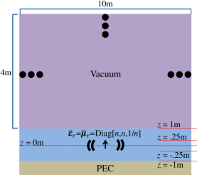
Figure 1: Vertically-oriented Hertzian dipole current source within a three-layer NBAM. The purple (air) and blue (NBAM) regions form the plane on which the fields are observed in Fig. 2. The parameter $n$ equals ten, five, and two within the regions $-1<z<-1/4$ [m], $-1/4<z<1/4$ [m], and $1/4<z<1$ [m], respectively.

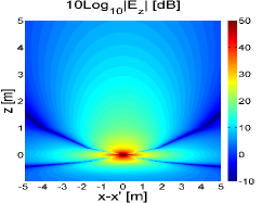
(a)

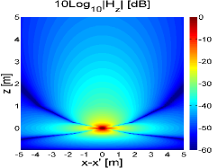
(b)

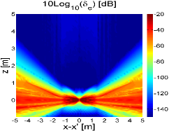
(c)

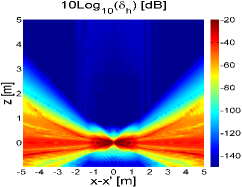
(d)

Figure 2: (a) $\mathcal{E}_{z}$ radiated by a VED. (b) $\mathcal{H}_{z}$ radiated by a VMD. (c) Relative error: $\mathcal{E}_{z}$. (d) Relative error: $\mathcal{H}_{z}$.

V Conclusion

We addressed a fundamental origination of breakdown in the spectral-domain-based (PWE) evaluation of EM fields radiated by sources embedded within NBAM planar slabs, leading to a robust formulation that can accurately compute EM fields despite the modal degeneracy, induced by said NBAM, that would ordinarily lead to numerical instabilities and/or corruption of the functional form of the plane wave eigenfunctions. Indeed this instability arises due to eigenvalues that, while non-defective, have an algebraic multiplicity equal to two rather than one. The remedy is to apply a proper (analytical) “pre-treatment” of the spectral-domain tensor operators prior to polarization amplitude extraction, resulting in robust analysis of EM fields in arbitrary anisotropic planar-layered media. Results validated the high accuracy of numerical computations based on this analytical pre-treatment.

References

- [1] K. Sainath, F. L. Teixeira, and B. Donderici, “Robust Computation of Dipole Electromagnetic Fields in Arbitrarily Anisotropic, Planar-Stratified Environments,” Phys. Rev. E, vol. 89, p. 013312, Jan 2014.
- [2] K. Sainath and F. L. Teixeira, “Tensor Green’s Function Evaluation in Arbitrarily Anisotropic, Layered Media using Complex-Plane Gauss-Laguerre Quadrature,” Phys. Rev. E, vol. 89, p. 053303, May 2014.
- [3] S. Lambot, E. Slob, and H. Vereecken, “Fast Evaluation of Zero-Offset Green’s Function for Layered Media with Application to Ground-Penetrating Radar,” Geophysical Research Letters, vol. 34, no. 21, pp. 1–6, 2007.
- [4] M. Rahm, S. A. Cummer, D. Schurig, J. B. Pendry, and D. R. Smith, “Optical Design of Reflectionless Complex Media by Finite Embedded Coordinate Transformations,” Physical Review Letters, vol. 100, p. 063903, Feb 2008.
- [5] D. Ye, Z. Wang, Z. Wang, K. Xu, B. Zhang, J. Huangfu, C. Li, and L. Ran, “Towards Experimental Perfectly-Matched Layers with Ultra-Thin Metamaterial Surfaces,” IEEE Transactions on Antennas and Propagation, vol. 60, no. 11, pp. 5164–5172, Nov 2012.
- [6] P. Boulanger and M. Hayes, “Electromagnetic Plane waves in Anisotropic Media: An Approach Using Bivectors,” Phil. Trans. Royal Society of London A: Mathematical, Physical and Engineering Sciences, vol. 330, no. 1614, pp. 335–393, 1990.
- [7] L. B. Felsen and N. Marcuvitz, Radiation and Scattering of Waves, ser. Electromagnetic Waves. Piscataway, NJ: IEEE Press, 1994.
- [8] K. A. Michalski, “Extrapolation Methods for Sommerfeld Integral Tails,” IEEE Transactions on Antennas and Propagation, vol. 46, no. 10, pp. 1405–1418, 1998.
- [9] G. W. Hanson and A. B. Yakovlev, Operator Theory for Electromagnetics. Springer, 2002.
- [10] T. A. Weber and C. L. Hammer, “A Note on Completeness,” Journal of Mathematical Physics, vol. 21, no. 1, pp. 24–27, 1980.
- [11] W. C. Chew, Waves and Fields in Inhomogeneous Media. Van Nostrand Reinhold, 1990.
- [12] K. Sainath and F. L. Teixeira, “Spectral-Domain-Based Scattering Analysis of Fields Radiated by Distributed Sources in Planar-Stratified Environments with Arbitrarily Anisotropic Layers,” Phys. Rev. E, vol. 90, p. 063302, Dec 2014.