Weak lensing reconstructions in 2D & 3D: implications for cluster studies

Abstract

We compare the efficiency with which 2D and 3D weak lensing mass mapping techniques are able to detect clusters of galaxies using two state-of-the-art mass reconstruction techniques: MRLens in 2D and GLIMPSE in 3D. We simulate otherwise-empty cluster fields for 96 different virial mass-redshift combinations spanning the ranges $3\times 10^{13}h^{-1}M_{\odot}\leq M_{vir}\leq 10^{15}h^{-1}M_{\odot}$ and $0.05\leq z_{\rm cl}\leq 0.75$, and for each generate 1000 realisations of noisy shear data in 2D and 3D. For each field, we then compute the cluster (false) detection rate as the mean number of cluster (false) detections per reconstruction over the sample of 1000 reconstructions. We show that both MRLens and GLIMPSE are effective tools for the detection of clusters from weak lensing measurements, and provide comparable quality reconstructions at low redshift. At high redshift, GLIMPSE reconstructions offer increased sensitivity in the detection of clusters, yielding cluster detection rates up to a factor of $\sim 10\times$ that seen in 2D reconstructions using MRLens. We conclude that 3D mass mapping techniques are more efficient for the detection of clusters of galaxies in weak lensing surveys than 2D methods, particularly since 3D reconstructions yield unbiased estimators of both the mass and redshift of the detected clusters directly.

1 Motivation

Current and upcoming large surveys such as the Dark Energy Survey (DES, The Dark Energy Survey Collaboration, 2005), Euclid (Refregier et al., 2010), and the Large Synoptic Survey Telescope (LSST, Ivezic et al., 2008; LSST Science Collaboration et al., 2009) will soon provide a large volume of high-quality weak lensing data covering a significant fraction of the sky up to redshifts $z\sim 2$. While the primary weak lensing science aims of these projects centre around the use of two-point statistics to constrain the cosmological parameters, there is nonetheless significant interest in reconstructing the mass distribution inferred by the lensing shear field. Such maps are obtained essentially for free in weak lensing surveys, as mass reconstruction algorithms require no additional data inputs to two-point shear statistics.

In addition to providing a valuable method for visualising the distribution of structure in the Universe, such maps can help to facilitate the computation of higher-order lensing statistics, in addition to providing a straightforward method to detect large structures such as clusters of galaxies. This can provide substantial insights into the nature and evolution of nonlinear structure in the Universe, and can help to break the degeneracy seen between cosmological parameters in constraints obtained from two-point shear statistics (e.g. Bernardeau, van Waerbeke & Mellier, 1997; Schneider et al., 1998; Takada & Jain, 2003, 2004; Jarvis, Bernstein & Jain, 2004; Kilbinger & Schneider, 2005; Pires et al., 2009; Bergé, Amara & Réfrégier, 2010; Dietrich & Hartlap, 2010; Pires, Leonard & Starck, 2012). Until very recently, weak lensing mass reconstruction efforts focused on estimating the two-dimensional projected mass density, the convergence $\kappa$, integrated along the line of sight. With the advent of accurate photometric redshift estimation methods and high-quality data, it has now become possible to consider reconstructing the full three-dimensional density field (Simon, Taylor & Hartlap, 2009; Simon et al., 2011; Simon, 2012; VanderPlas et al., 2011). One advantage to this approach is that, by directly reconstructing the density field, we might expect to be able to directly estimate the masses of haloes detected without relying on assumptions about the dynamical state of the halo. In a recent publication, Leonard, Lanusse & Starck (2014) demonstrated a sparsity-based approach to 3D lensing mass reconstructions (see also Leonard, Dupé & Starck, 2012) that is able not only to detect massive clusters of galaxies, but also to estimate their masses and redshifts in an unbiased way. This represents the first method able to reconstruct the density field from weak lensing measurements sufficiently accurately to allow direct estimates of the properties of dark matter haloes detected.

Such reconstructions, if sufficiently sensitive, might therefore be able to augment and complement optical cluster studies that aim to identify and weigh clusters of galaxies by considering the distribution and/or dynamics of the cluster members (e.g. Girardi et al., 1998; Łokas & Mamon, 2003; Łokas et al., 2006; Mamon & Boué, 2010; Falco et al., 2014). Clusters of galaxies are a very important cosmological probe. Studying the evolution of the cluster mass function (Rosati, Borgani & Norman, 2002; Voit, 2005), allows us to constrain both the amplitude of the power spectrum at the cluster scale and the linear growth rate of density perturbations. In addition, the clustering properties of the large-scale distribution of clusters provides direct information on the shape and amplitude of the underlying dark matter distribution and power spectrum (Borgani & Guzzo, 2001; Moscardini, Matarrese & Mo, 2001).

In this paper, we focus on two state-of-the-art weak lensing mass reconstruction techniques: GLIMPSE in 3D (Leonard, Lanusse & Starck, 2014) and MRLens in 2D (Starck, Pires & Réfrégier, 2006). The methodology underpinning the MRLens algorithm is qualitatively similar to that of GLIMPSE: both methods use wavelets, and impose sparsity to regularise the reconstructions and to control noise peaks. Other reconstruction methods in 2D could, of course, be chosen. An obvious example is the aperture mass statistic, which is frequently used for 2D mass mapping and peak detection. However, it was demonstrated in Leonard, Pires & Starck (2012) that the aperture mass statistic is formally identical to the wavelet transform of the convergence map, with the added advantages that

1. the wavelet transform considers several angular scales simultaneously, while application of the aperture mass statistic requires the choice of a scale radius,

2. the wavelet transform is between 10 to 1000 times faster depending on the scale (Leonard, Pires & Starck, 2012), and

3. the wavelet function intrinsically has some desirable properties, such as regularity, and compact support, and as a compensated filter it does not require truncation, unlike some aperture mass filters (see Leonard, Pires & Starck, 2012; Pires, Leonard & Starck, 2012, and references therein).

It was further shown in Pires, Leonard & Starck (2012) that MRLens produces 2D reconstructions that are more robust to noise peaks than the aperture mass statistic, and are therefore more useful for cosmological studies such as those involving peak counts. It was aso shown that MRLens outperforms other convergence reconstruction methods such as inverse Wiener filtering (Starck, Pires & Réfrégier, 2006). For these reasons, and given the similarity to GLIMPSE in its wavelet- and sparsity-based approach, MRLens seemed the natural choice of algorithm for such a comparison.

We examine the ability of weak lensing mass reconstruction techniques in two- and three-dimensions to detect clusters as a function of the cluster mass and redshift. Using simulated data, we consider 96 samples in virial mass and redshift $[M_{vir,j},z_{j}]$, $j=\{1..96\}$, and for each generate 1000 noise realisations. We generate reconstructions of these noisy fields using MRLens and GLIMPSE, and consider both the probability of detecting a real cluster of a given mass and redshift (the true detection rate), and the probability of finding a peak in a given field that arises due to noise (the false detection rate). Comparing the true detection rate in 2D and 3D reconstructions at the same peak signal-to-noise threshold allows us to probe any intrinsic differences in the lensing signal-to-noise when the full 3D information is retained versus when this information is projected along the line of sight. However, naively we might expect the false detection rate to scale with the number of pixels in the reconstruction, which is always larger in 3D than in 2D. The ideal reconstruction algorithm will maximise the true detection rate and minimise the false detection rate, and we examine how these compare between the two algorithms, and scale as a function of user-specified algorithm parameters.

This paper is organised as follows: In § 2, we provide a brief overview of weak lensing mass reconstructions, and outline the MRLens and GLIMPSE algorithms. In § 3 we describe the suite of cluster simulations, and present the results of our study as described above. We conclude with a brief discussion of our results and their implications for cluster and weak lensing surveys in § 4.

2 Mass Reconstruction Methods

In what follows, we assume that the vector

$$\mathbf{\gamma}^{(i)}=\left(\epsilon_{1}^{(i)}\epsilon_{2}^{(i)}...\epsilon_{N_{g}}^{(i)}\right)^{t}$$ (1)

contains the complex ellipticities of galaxies in a tomographic weak lensing survey binned on a grid with $N_{g}$ grid points. Sources are binned together on the angular grid only if they belong to the same redshift bin, which is denoted by the superscript ⁽ⁱ⁾ in equation (1) above. We can express the full three-dimensional weak lensing information as the vector $\mn@boldsymbol{\gamma}\equiv(\mn@boldsymbol{\gamma}^{(1)},\mn@boldsymbol{\gamma}^{(2)},...,\mn@boldsymbol{\gamma}^{(N_{z})})$, where $N_{z}$ is the number of redshift bins in the survey.

The aim of mass reconstruction methods is to relate the measured shear $\mn@boldsymbol{\gamma}$ to the underlying density distribution. Typically, in 2D, we aim to recover the projected, dimensionless surface density (the convergence) $\mn@boldsymbol{\kappa}^{(i)}$ from the tomographic shear $\mn@boldsymbol{\gamma}^{(i)}$, while in 3D we seek the dimensionless 3D matter overdensity $\mn@boldsymbol{\delta}$. We can relate the tomographic shear $\mn@boldsymbol{\gamma}^{(i)}$ to the convergence $\mn@boldsymbol{\kappa}^{(i)}$ of the lens by

$$\boldsymbol{\gamma}^{(i)}(\theta)=\frac{1}{\pi}\int d^{2}\theta^{\prime}\mathcal{D}(\theta-\theta^{\prime})\boldsymbol{\kappa}^{(i)}(\theta^{\prime})\ ,$$ (2)

where $\theta=\theta_{1}+\mathrm{i}\theta_{2}$ represents the angular coordinate on the sky, represented in complex notation,

$$\mathcal{D}(\theta)=\frac{1}{(\theta^{\ast})^{2}}\ ,$$ (3)

and the asterisk ^∗ represents complex conjugation.

Equation (2) represents a linear mapping between the shear and the convergence, and can be expressed in matrix notation as $\mbox{\boldmath{$\gamma$}}^{(i)}=\mathbf{P}_{\gamma\kappa}\mbox{\boldmath{$\kappa$}}^{(i)}+\boldsymbol{n}_{\gamma}^{(i)}$, where $\mn@boldsymbol{n}_{\gamma}^{(i)}$ is a vector of intrinsic source ellipticities and the linear transform $\mathbf{P}_{\gamma\kappa}$ is, for $\ell\neq m$:

$$[\mathbf{P}_{\gamma\kappa}]_{\ell m}=-\frac{A}{\pi}\frac{1}{[\theta_{\ell m}^{\ast}]^{2}}\ ,$$ (4)

where $A$ represents the solid angle of the angular grid pixels, and $\ell$ and $m$ give the $x$ and $y$ coordinates of the pixel on the grid. When $\ell=m$, we set $\mathbf{P}_{\gamma\kappa}=0$.

The underlying convergence, though representing a two-dimensional projected density, is actually itself a three-dimensional field: at each point $\boldsymbol{r}$ in three-dimensional space, we can compute a convergence $\mbox{\boldmath{$\kappa$}}(\boldsymbol{r})$, by considering the relationship of the lensing convergence to the underlying matter overdensity $\boldsymbol{\delta}(\boldsymbol{r})$. Note that we often parameterise the 3D position vector $\boldsymbol{r}$ in observations by an angular position $\theta$ and a redshift $z$. This matter overdensity, or density contrast, is defined as $\boldsymbol{\delta}(\theta,z)\equiv(\boldsymbol{\rho}(\theta,z)-\overline{\rho(z)})/\overline{\rho(z)}$, where $\boldsymbol{\rho}(\theta,z)$ is the density at angular position $\theta$ and redshift $z$ and $\overline{\rho}(z)$ is the mean matter density at redshift $z$, and is related to the convergence by

$$\small\mbox{\boldmath{$\kappa$}}(\theta,z)=\frac{3H_{0}^{2}\Omega_{M}}{2c^{2}}\int_{0}^{w}dw^{\prime}\frac{f_{K}(w^{\prime})f_{K}(w-w^{\prime})}{f_{K}(w)}\frac{\boldsymbol{\delta}[f_{K}(w^{\prime})\theta,w^{\prime}]}{a(w^{\prime})}\ ,$$ (5)

where $H_{0}$ is the hubble parameter, $\Omega_{M}$ is the matter density parameter, $c$ is the speed of light, $a(w)$ is the scale parameter evaluated at comoving distance $w$, and

$$f_{K}(w)=\begin{cases}K^{-1/2}\sin(K^{1/2}w),&K>0\\ w,&K=0\\ (-K)^{-1/2}{\rm sinh}([-K]^{1/2}w)&K<0\end{cases}\ ,$$ (6)

gives the comoving angular diameter distance as a function of the comoving distance and the curvature, $K$, of the Universe. $f_{K}(w)\theta$ in the argument of $\mn@boldsymbol{\delta}$ in equation (5) therefore gives the transverse comoving distance. If we now consider that we have a tomographic measurement of the convergence, $\mn@boldsymbol{\kappa}=(\mn@boldsymbol{\kappa}^{(1)},\mn@boldsymbol{\kappa}^{(2)},...,\mn@boldsymbol{\kappa}^{(N_{z})})$, obtained from the tomographic shear $\gamma$, the above relationship can also be expressed in matrix notation as $\mbox{\boldmath{$\kappa$}}=\mathbf{Q}\mbox{\boldmath{$\delta$}}$, where $\mathbf{Q}$ represents the line of sight convolution operation in equation (5), and is given in full in Simon, Taylor & Hartlap (2009) and Leonard, Lanusse & Starck (2014), and $\delta$ now represents a binned map of the density contrast. For a given set of shear measurements $\mn@boldsymbol{\gamma}$, we therefore can write

$$\gamma = \mathbf{P}_{\gamma\kappa}\mbox{\boldmath{$\kappa$}}+\boldsymbol{n}_{\gamma}\ ,$$ (7)

$$= \mathbf{P}_{\gamma\kappa}\mathbf{Q}\mbox{\boldmath{$\delta$}}+\boldsymbol{n}_{\gamma}\ ,$$ (8)

where, following the conventions used previously, $\mn@boldsymbol{n}_{\gamma}=(\mn@boldsymbol{n}_{\gamma}^{(1)},\mn@boldsymbol{n}_{\gamma}^{(2)},...,\mn@boldsymbol{n}_{\gamma}^{(N_{z})})$ represents the error in the shear measurements. While there are various sources of error in shear measurements, for the purposes of this paper we consider only noise arising from the intrinsic shapes of galaxies, which is typically taken to be a Gaussian distribution of width $\sigma_{\gamma}\sim 0.2-0.3$.

The task of mass reconstruction methods is the inversion of either equation (7) in 2D or equation (8) in 3D. Note that the formalism presented above assumes the absence of intrinsic alignments, and this assumption is propagated throughout the analysis. A full assessment of the impact of intrinsic alignments on the reconstruction quality is the subject of future work.

We outline below the methods underlying two state-of-the-art mass reconstruction techniques: MRLens (Starck, Pires & Réfrégier, 2006) in 2D and GLIMPSE (Leonard, Lanusse & Starck, 2014) in 3D.

2.1 2D mapping with MRLens

In 2D, our aim is to solve Equation (7) for each tomographic redshift bin and estimate the convergence $\mbox{\boldmath{$\kappa$}}^{(i)}$ from noisy shear measurements. In the Fourier plane, the convergence can be computed from the shear components as (Kaiser & Squires, 1993)

$$\tilde{\mbox{\boldmath{$\kappa$}}}^{(i)}(\mathbf{k})=\tilde{P}_{1}(\mathbf{k})\tilde{\mbox{\boldmath{$\gamma$}}_{1}}^{(i)}+\tilde{P}_{2}(\mathbf{k})\tilde{\mbox{\boldmath{$\gamma$}}_{2}}^{(i)},$$ (9)

where the hat symbol denotes Fourier transforms and we have defined $k^{2}\equiv k_{1}^{2}+k_{2}^{2}$ and

$$\tilde{P_{1}}(\mathbf{k}) = \frac{k_{1}^{2}-k_{2}^{2}}{k^{2}}$$

$$\tilde{P_{2}}(\mathbf{k}) = \frac{2k_{1}k_{2}}{k^{2}},$$ (10)

with $\tilde{P_{1}}(\mathbf{k})\equiv 0$ when $k_{1}^{2}=k_{2}^{2}$, and $\tilde{P_{2}}(\mathbf{k})\equiv 0$ when $k_{1}=0$ or $k_{2}=0$. These conditions on $\tilde{P_{1}}$ and $\tilde{P_{2}}$ when $k_{1}=k_{2}=0$ correspond to an indetermination of the mean value of the convergence field $\kappa$, known as the mass-sheet degeneracy. Applying an inverse Fourier transform on $\tilde{\kappa}$ estimated by equation (9) yields an estimate of the convergence. As this estimate is typically very noisy, some type of filtering or regularisation is usally included in a reconstruction algorithm in order to minimise the contaminating effect of noise on the resulting reconstruction. Gaussian and Wiener filtering are common choices, but may not be optimal, particularly since Wiener filtering is only optimal when both the signal and noise are Gaussian-distributed, and their power spectra are known.

MRLens is a Multi-Resolution Entropy filtering method using a wavelet based prior for the entropy to regularise the solution. For full details of the MRLens algorithm, the reader is referred to Starck, Pires & Réfrégier (2006); briefly, this method assumes that the reconstructed convergence can be represented sparsely when projected onto a well-chosen dictionary or set of functions (basis or frame). By this we mean that most of the information content can be captured by a small number of coefficients in the chosen dictionary or frame. For example, a periodic signal would be sparse in the Fourier domain, as it would be completely represented by a small number of Fourier coefficients. In the present case, we choose wavelets.

In the case of Gaussian noise, one can construct a multiresolution support in the wavelet domain by identifying as “significant” those wavelet coefficients $w_{j,\ell,m}$ that verify $|w_{j,\ell,m}|>k\sigma_{j}$, where $\sigma_{j}$ is the noise standard deviation at a particular wavelet scale $j$, and the indices $[\ell,m]$ again denote the pixel location in the 2D convergence map. The noise standard deviation can be estimated directly from the noisy map, and we typically choose the threshold $k$ to be between 3 and 5. Coefficients that are deemed thus to be significant are retained in the reconstruction, while an entropy based regularisation is applied to those coefficients that are not significant. An estimate of the convergence is built iteratively, through application of this regularisation on the residual between the data and the current convergence estimate.

2.2 3D mapping with GLIMPSE

The full 3D problem presents an additional difficulty compared to the 2D problem as we are trying to de-project the structures along the line of sight. However, the radial lensing operator $\mathbf{Q}$ is singular and leads to an ill-posed inverse problem, which does not accept a single, stable, solution even in the absence of noise. A robust method to address this very general class of problems is sparse regularisation, as in the 2D case, above. If the signal to recover is assumed to be sparse (only a small number of coefficients are non-zero) in an adapted dictionary, then a robust estimate of the original signal can be recovered by solving a optimisation problem with a penalty on the $\ell_{1}$ norm of the coefficients of the signal in the chosen dictionary (Starck, Murtagh & Fadili, 2010). GLIMPSE implements this approach in the context of the 3D mapping problem and recovers an estimate of the density contrast $\delta$ as the solution of the following minimisation problem:

$$\centering\min_{\boldsymbol{\alpha}}\frac{1}{2}\parallel\mbox{\boldmath{$\gamma$}}-\mathbf{P}_{\gamma\kappa}\mathbf{Q}\mathbf{\Phi}\mbox{\boldmath{$\alpha$}}\parallel^{2}_{\mathbf{\Sigma}}+\lambda\parallel\mbox{\boldmath{$\alpha$}}\parallel_{1}\ ,\@add@centering$$ (11)

where $\alpha$ are the coefficients of the estimate of the density contrast $\delta$ in an appropriate dictionary $\mathbf{\Phi}$ (i.e. $\mbox{\boldmath{$\delta$}}=\mathbf{\Phi}\mbox{\boldmath{$\alpha$}}$), $\lambda$ is a parameter tuning the sparsity constraint and, as before, $\mathbf{\Sigma}$ is the covariance matrix of the noise, assumed to be Gaussian. The first term in equation (11) is called the data fidelity term, and represents the $\ell_{2}$ distance between the data and the current estimate of the solution, weighted by the noise covariance, while the second term represents a sparsity penalty, i.e. the equation above is minimised when the $\ell_{1}$ norm of the vector of coefficients is as small as possible whilst being as close as possible to the input data.

GLIMPSE uses a 2D-1D dictionary for $\mathbf{\Phi}$ composed of isotropic wavelets in the 2D angular domain and Dirac delta functions in the radial dimension. Such a representation is well adapted to the expected density contrast of a typical dark matter halo, which is always contained within a single redshift bin given the resolutions we are able to attain in the radial dimension.

GLIMPSE solves this optimisation problem using a variant of the Fast Iterative Soft Thresholding Algorithm (FISTA, Beck & Teboulle (2009)). This algorithm relies on two steps, first the coefficients $\alpha$ of the solution are updated according to a gradient descent of the data fidelity term, then the coefficients are thresholded, setting to zero coefficients of amplitude lower than $\lambda$. This imposes the sparsity constraint on the solution. As with MRLens, GLIMPSE sets the threshold level to $\lambda_{j,n}=k\sigma_{j,n}$ where $\sigma_{j,n}$ is the noise standard deviation at wavelet scale $j$ and redshift bin $n$. With this choice of parameter, at each iteration only the significant coefficients (i.e. of amplitude above $k\sigma_{j,n}$) are allowed to enter the solution. The only parameter to set for the GLIMPSE algorithm is the significance threshold $k$; as with MRLens, this is usually taken to be between 3 and 5.

3 Tests with cluster simulations

In order to test the effectiveness of the two mapping techniques at detecting and reconstructing clusters of galaxies, we simulated 96 clusters of galaxies at a range of masses and redshifts as in Leonard, Lanusse & Starck (2014); Figure 1 shows the points sampled in virial mass-redshift space. Each cluster halo follows an NFW profile (Navarro, Frenk & White, 1997) with a concentration parameter computed from the virial mass and redshift using the parameterisation given in Coupon et al. (2012).

From the NFW density profile, we computed the corresponding shear signal, which is derived analytically in Takada & Jain (2003). The computations required to simulate the halos were performed making extensive use of the NICAEA software package, using a flat $\Lambda$CDM cosmology with $\Omega_{\rm M}=0.264,\ \Omega_{\Lambda}=0.736$, and $H_{0}=71$km/s/Mpc.

Figure 1: This figure shows the virial mass and redshift for the 96 clusters forming this study.

Each cluster was simulated in an otherwise empty field with an angular pixel size of $1^{\prime}\times 1^{\prime}$. We considered our shear information to come from galaxies following a uniform angular distribution on the sky, with a redshift distribution given by

$$n(z)=z^{\alpha}\exp\left(-\left[\frac{z}{z_{0}}\right]^{\beta}\right)\ ,$$ (12)

where we take $z_{0}=1/1.4$, giving a median redshift $z_{\rm med}=1$, $\alpha=2$ and $\beta=1.5$ for a Euclid-like survey (Taylor et al., 2007; Kitching, Heavens & Miller, 2011). We assumed 30 galaxies per square arcminute, and that the intrinsic galaxy ellipticity follows a Gaussian distribution of width $\sigma_{\varepsilon}=0.25$. In their current forms, both MRLens and GLIMPSE take as inputs the shear, rather than the reduced shear ($g=\gamma/(1-\kappa)$), and so our simulations produce noisy shear fields, rather than reduced shear fields. This is a simplification, included simply for ease of computation of our simulations, but which may lead to a biased reconstruction if applied to real data. However, Jullo et al. (2014) describe an iterative scheme to account for the reduced shear that converged after three iterations and de-biases the reconstruction. Such an iterative process can be implemented with both MRLens and GLIMPSE in applications to real data to account for reduced-shear. This will be demonstrated for GLIMPSE in future work.

Finally, we assumed Gaussian photometric redshift errors with a standard deviation given by $\sigma_{z}=0.05(1+z)$ and no bias.

The 2D projected shear map was computed by integrating the lensing signal along each line of sight, while the 3D shear map was computed using 30 tomographic bins of variable width $\Delta z$, such that each tomographic bin contained the same number of galaxies. The bins were chosen to be sequential in photo-z space. Given the photometric redshift errors, such a choice means that the true redshift distributions for each bin overlap (see, e.g., figure 2 of Leonard, Lanusse & Starck, 2014). Each map was generated with $64\times 64$ angular pixels, each of width $\delta\theta=1$ arcmin. In order to properly asses the statistics of the reconstructions, for each cluster field, we computed 1000 noisy realisations of the data.

3.1 Algorithm configurations

In order to compare the two methods in a fair way, we used algorithm configurations that were as similar as possible. Both MRLens and GLIMPSE were run using the same 2D wavelets (the starlet, Starck, Fadili & Murtagh, 2007) using 6 wavelet scales in the decomposition. As GLIMPSE applies a $k\sigma$ hard threshold in density space, we configured MRLens to use $k\sigma$ thresholding, rather than the default False Discovery Rate (FDR) thresholding. This is not the optimal configuration for MRLens, as it may allow a higher fraction of false peaks to appear in a given reconstruction, but was chosen in order to provide a fair basis for comparison with GLIMPSE. The threshold level was chosen to be at 4$\sigma$ for GLIMPSE. For MRLens, we considered three different thresholds: $3\sigma,\ 3.5\sigma,\ \mathrm{and}\ 4\sigma$.

In this paper, we are interested in both the probability of detecting a real cluster of a given mass and redshift with a given denoising threshold(the true detection rate), and the probability of finding a peak in a given field that rises above the denoising threshold but is due entirely to noise (the false detection rate). Comparing the true detection rate between 2D reconstructions and 3D reconstructions at the same denoising threshold will probe any intrinsic differences in the lensing signal to noise when the signal is projected in 2D vs when the full 3D information about the signal is retained. However, naively we expect the false detection rate at a fixed denoising threshold to scale with the number of pixels in the reconstruction, and therefore naturally expect a higher level of contamination from spurious peaks in a 3D reconstruction of a given lensing field than in the 2D reconstruction of that field using the same denoising threshold.

A mass reconstruction algorithm will ultimately be judged both on its ability to detect real clusters and its effectiveness at controlling spurious peaks. There is always a trade-off to be had between completeness, which may be increased by lowering the denoising threshold, and purity, which is improved by raising the denoising threshold. The setup of the present experiment does not allow us to compute the expected purity we might obtain in a reconstruction of a real weak lensing dataset. However, a comparison of the true detection rates obtained by MRLens and GLIMPSE when the denoising thresholds yield comparable false detection rates provides a more fair assessment of the overall performance of the two methods in application to weak lensing studies.

3.2 Peak identification

We used CLFIND (Williams, de Geus & Blitz, 1994), which is a friends-of-friends algorithm, to identify connected pixels above a given threshold associated with a possible detection. The user is required to set a minimum value that a pixel can have in order to be considered as part of a detected structure. The aim is to identify the pixels associated with a detected peak out to large radii from the centre of that peak, so that we are able to accurately compute properties such as the density-weighted centroid for the detected peak.

Setting the detection threshold in 3D is fairly straightforward: the GLIMPSE algorithm applies thresholding to the solution, meaning that regions of the reconstruction in which there are deemed to be no significant coefficients during the iterative reconstruction process will be set to zero in the reconstruction. Therefore, any deviations from zero may be considered a detection of a feature above the noise. However, setting the CLFIND threshold to be zero can lead to blending of detected structures and an increased runtime for the algorithm, so to minimise any potential blending and to optimise the runtime of the CLFIND algorithm in 3D, we set the detection limit to be $\delta_{min}=1$.

Defining a detection in 2D is somewhat more complicated. While MRLens does apply hard thresholding during the iterative procedure, due to differences in the details of the algorithm – specifically, that MRLens computes the multiresolution support and applies the entropy based regularisation to the residual, which is then added back on each iteration to build the solution – there are no regions in the reconstructed convergence maps that are identically zero. Furthermore, due to the mass-sheet degeneracy, the overall normalisation of the reconstructed convergence map may be somewhat arbitrary. In practice, this is usually constrained by either setting the mean convergence (over a sufficiently large field) to be zero or, in cluster fields, by setting the convergence to be zero sufficiently far away from the cluster. We apply no such boundary conditions in the 2D reconstructions presented here. However, we note that in 3D the density contrast is naturally physically constrained to be $\geq-1$ (i.e. the density is always positive), and GLIMPSE applies a positivity constraint to its estimate of the solution at each iteration.

To ensure that we all the structures identified in the multiresolution support and no others, we perform a multi-step detection procedure on all the 2D reconstructions (see figure 2 for illustrations of each step):

1. Identify all pixels in the convergence reconstruction (figure 2(a)) where the multiresolution support (figure 2(b)) is non-zero; find the minimum value of the convergence amongst these pixels, $\kappa_{min}$. We define $\kappa_{lim}=\min[3\times 10^{-3},\kappa_{min}/2]$.

2. Search for all pixels with values $\geq\kappa_{lim}$ that are connected to the pixels with non-zero multiresolution support.

3. Mask all other pixels (figure 2(c)).

4. Run CLFIND on the masked map to identify and separate the peaks detected in the map (figure 2(d))

Note that the limiting value of $3\times 10^{-3}$ above was chosen as an effective trade-off between capturing as many pixels as possible associated with each peak detected and minimising blending and the CLFIND algorithm runtime. In cases where the convergence value at the locations of non-zero multiresolution support are close to this value, the limit is lowered in order to link a larger number of pixels to the detected peaks. This also ensures that peaks coinciding with non-zero multiresolution support are always detected. This does occasionally lead to blending, however CLFIND as the final step is able to isolate and separate blended peaks where two clear local maxima occur.

(a) The reconstructed convergence produced by MRLens, plotted on a logarithmic colour scale.

(b) The multiresolution support produced by MRLens, showing the pixel locations at which a significant wavelet coefficient was detected.

(c) Pixels not connected with regions of non-zero multiresolution support are masked and CLFIND run on the resulting image as illustrated above. We use here the same colour scheme as in figure 2(a) above.

(d) The output from CLFIND: a mask identifying and labelling distinct structures in the reconstruction. The pixels associated with each clump are used to compute the convergence-weighted centroid of the peak.

Figure 2: The pipeline for detection of peaks in 2D MRLens reconstructions . The 3D pipeline is simpler, involving application of CLFIND directly on the 3D reconstructions, with no masking required.

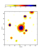
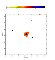
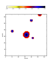
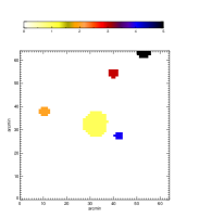
We compute the location of each peak in 3D by computing the density-weighted centroid $[x,y,z]$, and in 2D analogously by computing the convergence-weighted centroid $[x,y]$ using those pixels identified by CLFIND.

3.3 Peaks arising from the noise

Naively, we expect that when we consider the angular distribution of all peaks detected in all 1000 reconstructions of a given cluster field, we will find a strong tendency to detect a peak in the centre of the field, where the cluster is located, and a roughly uniform distribution of false peaks arising from the noise, at a much lower amplitude. This is because false detections due to random noise are expected to be uniformly randomly distributed, as the noise is uniform and uncorrelated in the $x-y$ plane.

In figure 3 we plot a histogram of the $x$ and $y$ positions of all detected peaks in 1000 GLIMPSE 3D reconstructions of a field containing a relatively high signal-to-noise cluster of virial mass $M_{vir}=7\times 10^{14}h^{-1}M_{\odot}$ located at a redshift of $z_{cl}=0.35$, and an analogous plot for reconstructions of a lower signal-to-noise cluster of $M_{vir}=9\times 10^{13}h^{-1}M_{\odot}$ at the same redshift. As expected, in both cases we see a concentration of detections around the centre of the image, and a roughly uniform background with the indication of some edge effects on the borders of the image.

Figure 3: This figure shows the distribution of the $x$ and $y$ positions of peaks detected in 1000 GLIMPSE 3D reconstructions of a field containing a cluster of virial mass $7\times 10^{14}h^{-1}M_{\odot}$ at a redshift of $z_{\rm cl}=0.35$ (left panel) and the analogous plots for a field containing a smaller cluster of virial mass $9\times 10^{13}h^{-1}M_{\odot}$ at the same redshift (right panel). In both cases, the central peak represents detections of the cluster itself, while the approximately uniform background represents false detections. Some edge effects are apparent at extreme values of $x$ and $y$.

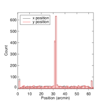
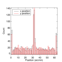
Figure 4 shows the comparable distribution of peaks from MRLens 2D reconstructions of the same fields. Histograms are plotted for the 3 different denoising thresholds as indicated in the legend. In all cases, there is a concentration of detections around the centre, as expected, and a background of false peaks. The amplitude of both the central peak and the uniform background of false detections decreases as the denoising threshold is raised. This is expected: the higher the threshold used, the more we will suppress the detection of peaks arising due to the noise. However, in doing this, we also reduce somewhat the probability that we will detect the central peak.

Figure 4: This figure shows the distribution of the $x$ positions ($y$ positions are assumed to be symmetrical) of peaks detected in 1000 MRLens 2D reconstructions of a field containing a cluster of virial mass $7\times 10^{14}h^{-1}M_{\odot}$ at a redshift of $z_{\rm cl}=0.35$ (left panel) and the analogous plots for a field containing a smaller cluster of virial mass $9\times 10^{13}h^{-1}M_{\odot}$ at the same redshift (right panel). In both cases, the different coloured histograms are derived using different values of the denoising threshold. This choice clearly impacts both the false and true detection rates.

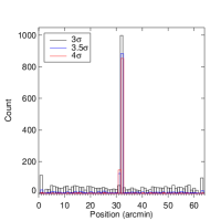
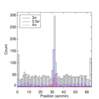
When the edge effects at extremal values of $x$ and $y$ are excluded, the distributions shown in figures 3 and 4 can be fit by a Gaussian plus a constant offset representing the uniform background of false detections. We carried out such fits for the distributions of $x$ and $y$ generated from the 1000 reconstructions of each cluster field using GLIMPSE, and for MRLens for each of the three denoising thresholds tested. In all but the lowest signal-to-noise cases, where the fitting procedure failed, the mean $x$ and $y$ identified by the fitting procedure were clustered around $[\overline{x},\overline{y}]=[32,32]$, and the standard deviations $\sigma_{x}$ and $\sigma_{y}$ were consistently found to be in the range $0.3-1.4$, with a trend to larger values of the standard deviation for fields with a lower signal to noise.

Given the difficulty of obtaining a reliable Gaussian fit for cluster fields where the rate of detection of the cluster is very low, we chose to define a cluster detection in both 2D and 3D as any detection with $30\leq x\leq 34$ and $30\leq y\leq 34$ in pixel units. Anything outside of this range is considered to be a false detection. This choice may artificially reduce the true detection count in lower signal-to-noise fields relative to those with higher lensing signal-to-noise; however, in the majority of cases, we retain as true detections those peaks lying within $2-4$ standard deviations from the mean position at the centre of the field. Moreover, the width of the $x-y$ distributions for a given cluster field were found to be very similar regardless of the reconstruction method and denoising threshold. Therefore, the choice to restrict detections of the cluster to those falling within the range $30\leq x\leq 34\ \&\ 30\leq y\leq 34$ does not unfairly (dis)advantage any particular method.

We also note in the figures that there appears to be an overdensity of detections near the edges of the reconstructions. In order to minimise the contamination from these edge effects in the analysis that follows, we exclude all false detections located within 4 pixels of the edge of the reconstruction in the transverse plane.

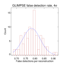
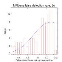
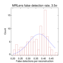
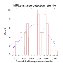
In figure 5, we show a histogram of the mean false detection rate per reconstruction seen in each of our 96 cluster fields using GLIMPSE, and using MRLens with denoising thresholds of $3\sigma$, $3.5\sigma$ and $4\sigma$. Overplotted in the figures are the best-fit Gaussian distributions. The fit parameters, the mean $\mu_{\rm fit}$ and the standard deviation $\sigma_{\rm fit}$ are listed in Table 1 and compared with the median and median absolute deviation (MAD) statistics computed from the 96 computed false detection rates.

Algorithm	Threshold	$\mu_{\rm fit}$	$\sigma_{\rm fit}$	Median	MAD
MRLens	3$\sigma$	2.087	0.357	1.923	0.231
MRLens	3.5$\sigma$	0.373	0.069	0.377	0.062
MRLens	4$\sigma$	0.056	0.018	0.056	0.018
GLIMPSE	4$\sigma$	0.781	0.047	0.786	0.044

Table 1: This table gives the parameters of the best-fit Gaussian to the distribution of the number of false detections per realisation in the 96 cluster fields analysed with MRLens at 3 different denoising thresholds and GLIMPSE at a denoising threshold of $4\sigma$. Also listed are the median and median absolute deviation (MAD) statistics computed from the 96 cluster field false detection rates.

We can clearly see that the MRLens false detection rate in 2D is substantially smaller (by a factor of $\sim 38$) than that seen in 3D at the same denoising threshold of $4\sigma$, and only becomes comparable to the $4\sigma$ GLIMPSE false detection rate when the denoising threshold drops between $3-3.5\sigma$. As noted in section 3.3, given that there are more pixels in 3D than in 2D, it is expected that we will have more false detections in 3D than in 2D for the same threshold level, so this result is unsurprising.

On the other hand, it does indicate that when assessing the overall performance of the GLIMPSE and MRLens algorithms it is not sufficient to simply look at their cluster detection rates at the same denoising threshold. In both cases, there will be a trade-off between increasing the cluster detection rate by lowering the denoising threshold, and controlling the false detection rate with a stricter choice of threshold. However, in 2D the false detection rate is naturally lower than in 3D, and therefore a lower threshold can be chosen in 2D than in 3D for the same level of false peak contamination.

For this reason, we compare the GLIMPSE results using a denoising threshold of $4\sigma$ with MRLens results at three different thresholds. Comparing the MRLens and GLIMPSE true detection rates when both use a $4\sigma$ threshold allows us to determine whether there is any intrinsic signal-to-noise advantage in studying lensing systems in 3D rather than 2D. Any information gained in 3D comes at the price of increased false detections, and so we lower the threshold in 2D so that the false detection rates become comparable between GLIMPSE and MRLens, to determine whether the information gain in 3D is sufficient to outweigh the increased false detections compared with what is achievable in 2D.

Figure 5: This figure shows the distribution of the mean false detection rate per reconstruction for the 96 cluster fields described in the text, reconstructed using GLIMPSE with a $4\sigma$ denoising threshold, and MRLens with denoising thresholds at $3\sigma$, $3.5\sigma$, and $4\sigma$.

3.4 Control of false detections

It is clear that spurious peaks arising from the noise may mimic real peaks in a reconstruction, and will therefore be a significant contaminant in any study that aims to constrain cosmological parameters using peak counts, or which aims to estimate the mass function. It is therefore important to consider strategies that might be implemented to remove these false detections or limit their impact on any resulting cosmological inference.

Figures 3 and 4 indicate that the distribution of false peaks is uniform across the field under randomisations to the underlying noise. While this is true in our idealised simulations, in which we have assumed a uniform distribution of background sources, real data often contains a complex gap structure and boundaries, which may give rise to a less uniform distribution of false peaks. We nonetheless expect that peaks arising due to the noise will not appear consistently in the same places under different, randomised realisations of the noise.

In practice, when applying either GLIMPSE or MRLens to real data, one would need to carry out Monte$-$Carlo or bootstrap resampling of the data in order to gain a full understanding of the noise properties of the reconstructed maps. Moreover, as demonstrated in Leonard, Lanusse & Starck (2014), a reliable estimate of the mass and redshift of a detected cluster, and their associated errors, can only be obtained by considering an ensemble of reconstructions carried out under randomisations to the noise in the data.

Figure 6: The mean of 1000 reconstructions in 2D (3$\sigma$ threshold; left panel) and 3D (4$\sigma$ threshold; right panel) of field 53, containing a cluster of mass $M_{vir}=7\times 10^{14}h^{-1}M_{\odot}$ and redshift $z_{\rm cl}=0.35$. Both plots use a logarithmic colour scheme, to accentuate any low-level false detections in the mean reconstruction. The detection rate for this cluster in both 2D and 3D at the chosen denoising thresholds is $100\%$.

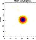
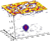
Given that false detections are randomly distributed, the probability of detecting a noise peak repeatedly in the same position under a different realisation of the noise is very low. In other words, we expect the ’detection rate’ associated with a given false detection at a position $[x,y,z]$ to be very low. One way to visualise this is to consider a mean reconstruction, obtained by summing the reconstructions obtained from the all 1000 realisations of the data.

A real cluster should be detected consistently at the same location and with a similar peak amplitude in (many of the) reconstructions using different realisations of the noise, so this feature should be prominent in such a mean map, while the false detections, which appear in random positions, will be suppressed by averaging many reconstructions.

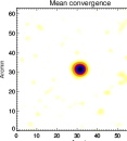
Figure 6 shows the mean 2D (3.5$\sigma$ threshold) and 3D (4$\sigma$ threshold) reconstructions of field 53. To highlight any low-level false detections, we plot the densities on a logarithmic colour scale. While this particular cluster has a detection rate of $\sim 100\%$ in both 2D and 3D, the mean density maps are typical for clusters with a much lower detection rate (e.g. figure 7, where we show the results for field 46, containing a cluster of mass $M_{vir}=9\times 10^{13}h^{-1}M_{\odot}$, redshift $z_{\rm cl}=0.35$, and detection rate $\sim 25\%$). In 2D, it is trivial to identify the location of the true density peak in the mean reconstruction: no other significant peaks are visible in the mean map.

In 3D, we notice several interesting features. Firstly, the cluster is clearly visible in the mean reconstruction, but appears to be smeared out in redshift. This is because the broad lensing efficiency kernel $\mathbf{Q}$ gives rise to a large uncertainty in the redshift at which the cluster is detected. This is evidenced by the large error bars seen in the redshift estimates for these clusters presented in Leonard, Lanusse & Starck (2014). The cluster is clearly defined, though, and no significant false detections are seen at redshifts below $z\lesssim 1.5$.

Figure 7: The mean of 1000 reconstructions in 2D (3.5$\sigma$ threshold; left panel) and 3D (4$\sigma$ threshold; right panel) of field 46, containing a cluster of mass $M_{vir}=9\times 10^{13}h^{-1}M_{\odot}$ and redshift $z_{\rm cl}=0.35$. Again, we use a logarithmic colour scheme. The detection rate for this cluster in both 2D and 3D at the chosen denoising thresholds is $\sim 50\%$.

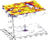
We do see the significant presence of high-amplitude false detections at the high-redshift boundary of the mean reconstruction, however. Such false detections were seen in Leonard, Dupé & Starck (2012) and Leonard, Lanusse & Starck (2014), and arise due to overfitting of the shear data in the highest redshift bins.

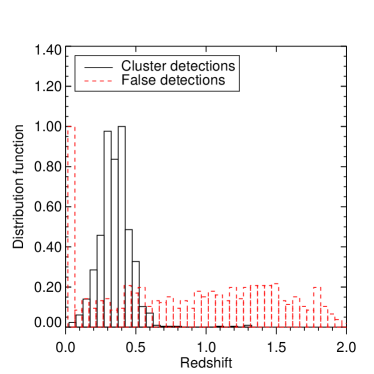
In figure 8, we plot the redshift distribution of the central cluster detections and the false detections for field 53. While the redshift distribution of the cluster detections shows an approximately Gaussian distribution centred on the true input redshift (in this case, $z_{\rm cl}=0.35$), the redshift distribution of the false detections shows a significant overdensity at very low and very high redshift, and a flat distribution in between. This distribution is characteristic of all the cluster fields studied. Given that we physically do not expect to see such a high density peak at such high redshifts, truncating the 3D reconstructions at $z=1.5$ will remove these high redshift false detections, which account for $\sim 30\%$ of all false detections seen in 3D, whilst having a minimal impact ($<2\%$ on the cluster detection rate).

Figure 8: The redshift distribution of cluster detections and false peaks in reconstructions of 1000 noisy realisations of shear data for field 53, containing a cluster of mass $M_{vir}=7\times 10^{14}h^{-1}M_{\odot}$, redshift $z_{\rm cl}=0.35$.

3.5 Cluster detection rate: 2D vs 3D

With false detections now well understood, we turn our attention to consider the detection rate expected for clusters as a function of mass and redshift for both MRLens and GLIMPSE. Figure 9 shows the fraction of noise realisations in which a given cluster was detected as a function of mass for each of the 8 different redshifts at which we simulated cluster haloes. This figure effectively shows the selection function for each method in the configurations specified above as a function of mass and redshift. Error bars were computed assuming Poisson noise only.

Figure 9: The fraction of noise realisations in which the central cluster was detected as a function of mass and redshift. 3D mapping clearly outperforms 2D mapping for detection of clusters for all but the highest mass clusters at which both methods asymptote to a detection rate of $100\%$.

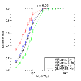
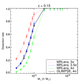
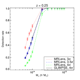
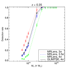
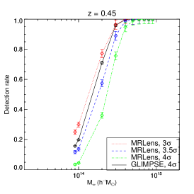
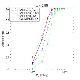
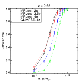
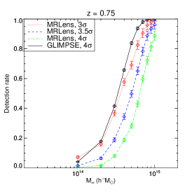
The selection functions in 2D and 3D all show the same general trends: an asymptote towards zero detections at low mass and an asymptote at high mass towards 100% detections. There is also a consistent trend towards lower detection rates at high redshift than low redshift for fixed cluster mass. However, these dependencies differ between 2D and 3D: GLIMPSE (4$\sigma$) vs MRLens (4$\sigma$):
This comparison offers insight into whether there is a natural signal-to-noise advantage in studying weak lensing clusters in 3D rather than 2D. In 26 fields, both GLIMPSE and MRLens have detection rates of $100\%$ (the GLIMPSE detection rate is $100\%$ in 39 of the cluster fields). In every other field, GLIMPSE outperforms MRLens in terms of detection rate. The largest improvement is seen for field 88, a $2\times 10^{14}h^{-1}M_{\odot}$ cluster at a redshift of $0.75$, where the GLIMPSE detection rate of 0.178 is a factor of 11.1$\times$ larger than that with MRLens (0.016). The GLIMPSE detection rate is $2\times$ higher than that of MRLens in 27 fields and $5\times$ in 6 fields. There therefore appears to be a natural advantage to using 3D reconstructions for cluster detection in weak lensing surveys.

However, as noted in section 3.1, comparing the GLIMPSE and MRLens detection rates at the same detection threshold is not an entirely fair comparison, as the GLIMPSE reconstructions show a $\sim 38\times$ higher rate of false detections than the MRLens 2D reconstructions at a $4\sigma$ threshold. A more fair comparison can be obtained by reducing the MRLens denoising threshold to a level such that the reconstructions show a similar rate of false detections. This level is reached at a threshold somewhere between $3-3.5\sigma$. GLIMPSE (4$\sigma$) vs MRLens (3.5$\sigma$):
The GLIMPSE false detection rate at $4\sigma$ is significantly closer (within a factor of $\sim 2$) to that of MRLens at $3.5\sigma$, so a comparison between these two sets of reconstructions is of particular interest. The detection rates in this case, particularly at low redshift, are quite similar. In 31 cluster fields, both MRLens and GLIMPSE attain a $100\%$ detection rate. In 17 cluster fields, the MRLens detection rate is higher than the GLIMPSE detection rate, but the difference is typically on the order of $5-10\%$, with the largest difference, $\sim 20\%$, seen in field 1 where the GLIMPSE detection rate is 0.134 and the MRLens detection rate is 0.161. As the cluster is moved to higher redshift, the detection rates in 3D become consistently higher than in 2D: in 48 fields, the GLIMPSE detection rate is higher than that of MRLens, and in 3 of those fields the improvement is greater than a factor of 2. Field 88 is again one of the fields in which the largest improvement is seen. In this case the GLIMPSE detection rate is $\sim 2.7\times$ larger than that of MRLens. GLIMPSE (4$\sigma$) vs MRLens (3$\sigma$):
Given that the false detection rate of GLIMPSE at $4\sigma$ remains significantly higher than that of MRLens at $3.5\sigma$, for completeness we again lower the MRLens denoising threshold to $3\sigma$. Here the MRLens false detection rate is $\sim 2.5\times$ larger than that of GLIMPSE. With such a low denoising threshold in 2D, we see a corresponding boost in detection rates, as expected. In this case, we find that both GLIMPSE and MRLens attain a $100\%$ detection rate in 34 cluster fields. In 44 of the cluster fields, the MRLens detection rate is higher than that of GLIMPSE. These are primarily at lower redshift, and the detection rates remain within a factor of $2$ for all but 4 of the fields. The largest difference is seen in field 15, where the MRLens detection rate (0.224) is $2.7\times$ larger than that of GLIMPSE (0.082). At higher redshift, we find that the GLIMPSE detection rate remains higher than that of MRLens in 20 of the cluster fields, but the improvement here is moderate (the ratio between the GLIMPSE and MRLens detection rates is typically of order $\sim 1.2$).

4 Discussion

The results above clearly demonstrate that mass mapping is a very useful tool for detecting clusters of galaxies in weak lensing surveys. At low redshift, GLIMPSE and MRLens provide reconstructions of comparable quality, when one considers both the cluster detection rate and the false detection rate seen in these reconstructions. However, GLIMPSE mapping offers a distinct advantage in the detection of clusters at high redshift, showing a significantly higher sensitivity to such clusters than seen in 2D with MRLens.

The improvement seen in 3D is likely due to a combination of effects. In projecting the data down into 2D, we lose some of the information content contained in the data. Additionally, particularly in the case of high redshift clusters, the lensing signal becomes damped when averaging galaxy shapes over the full range of redshifts probed by the survey: in our experiment, the average ellipticity in each angular pixel $[x,y]$ is given by

$$\epsilon(x,y)=\frac{\int_{0}^{2}p(z)\gamma(x,y,z)dz}{\int_{0}^{2}p(z)dz}+\mathcal{N}(0,\sigma_{\varepsilon}/\sqrt{n})\ ,$$ (13)

where $\gamma(x,y,z)$ is in this case the analytically-derived shear at angular position $[x,y]$ and redshift $z$, $p(z)\propto n(z)$ gives the probability distribution function for the galaxies in the survey and $\mathcal{N}$ is a random noise contribution drawn from a Gaussian of mean 0 and standard deviation $\sigma_{\varepsilon}/\sqrt{n}$, where $n$ is the number of galaxies per pixel. In practice, in a real galaxy survey, equation (13) will be replaced by a discrete sum over galaxy ellipticities.

Clearly, the lensing signal $\gamma(x,y,z)\equiv 0\ \forall z<z_{\rm cl}$, where $z_{\rm cl}$ is the redshift of the cluster. If the cluster redshift is known a priori, one can retain only those galaxies behind the cluster; however in the absence of this knowledge, computing a 2D shear map by averaging over all the galaxies in a survey will result in a damping of the lensing signal due to the inclusion of galaxies that are not lensed, and this effect will be more pronounced for higher redshift clusters.

The GLIMPSE 3D reconstruction method is significantly more sensitive than the state-of-the-art 2D reconstruction algorithm MRLens, particularly for clusters at low mass and/or at high redshift. At low redshift, the quality of GLIMPSE and MRLens reconstructions are comparable. The false detection rates are similar between GLIMPSE and MRLens at $3.5\sigma$, and the detection rates align similarly: GLIMPSE exhibits a detection fraction above $\gtrsim 50\%$ for clusters of mass $M_{vir}\gtrsim 10^{14}h^{-1}M_{\odot}$ at low redshift ($z\sim 0.25$); MRLens provides a comparable detection rate at a $3.5\sigma$ at this redshift with the detection rates at $3\sigma$ and $4\sigma$ being $70\%$ and $30\%$, respectively. At high redshift, there is a clear improvement in 3D reconstructions. For example, GLIMPSE detects $63\%$ of clusters of mass $3\times 10^{14}h^{-1}M_{\odot}$, while the MRLens detection rates are $59\%\ (3\sigma),\ 37.5\%\ (3.5\sigma)\mbox{ and }19\%\ (4\sigma)$. At high redshift, where the weak lensing signal-to-noise is low, it is therefore significantly advantageous to employ GLIMPSE for the detection of clusters in weak lensing maps.

We have demonstrated that MRLens and GLIMPSE can be tuned to yield mass reconstructions with similar levels of purity; in other words, reconstructions in which the contamination due to peaks arising from the noise is at a similar level in both 2D and 3D reconstruction methods. Given the findings of Pires, Leonard & Starck (2012) that peak counts undertaken on MRLens reconstructions provide a powerful method to probe non-Gaussianity and to discriminate between degenerate cosmological models, it is reasonable to expect that 3D reconstructions with GLIMPSE will offer an even more powerful constraint on non-Gaussianity, given the higher levels sensitivity to high-redshift clusters seen in GLIMPSE reconstructions.

Furthermore, as described in Leonard, Lanusse & Starck (2014), GLIMPSE reconstructions provide an unbiased estimator of both the masses and redshifts of the clusters detected. We expect that the selection function for optical halo finders will differ somewhat from that of GLIMPSE, but a detailed comparison would require a sophisticated simulation involving N-body cosmological simulations, raytracing, and a realistic semi-analytic modelling of galaxy formation. This comparison will be the subject of future work, and has implications for the study of galaxy clusters and their statistics in large upcoming surveys such as Euclid.

A final cosmological application of GLIMPSE would be to measure the evolution of the high-mass end of the mass function. To do this, we need an accurate model of the GLIMPSE selection function as a function of cluster mass, redshift, and concentration parameter, and also as a function of the underlying cosmological model. Work is ongoing in this area, and will be the subject of an upcoming publication. GLIMPSE is a non-parametric reconstruction method, which means that we do not compute a virial mass or redshift for the clusters we detect as part of the algorithm, but rather compute masses by integrating the density over a range of pixels in the reconstruction. In order to use GLIMPSE outputs to compute the cluster mass function, we must first be able to translate the GLIMPSE masses into virial masses, or to model the mass function for the GLIMPSE observables as a function of virial mass, redshift and cosmological model. This task is not trivial, but certainly feasible.

It is important to note that the simulations presented here are highly idealised, and that real data will pose many additional challenges. The data themselves will contain complicated shear and photometric redshift systematics, and the effects of more complicated (and possibly correlated) errors, biases, and photometric redshift catastrophic failures, as well as the impact of intrinsic alignments, on the resulting mass maps will need to be investigated.

Moreover, a more realistic density distribution containing clustered mass peaks will result in blending of structures in mass maps, and thereby impact the measured peak counts and/or cluster mass function. In a very preliminary work, Leonard, Dupé & Starck (2012) demonstrated that sparsity-based 3D mapping techniques may be able to disentangle different density peaks located along the same line of sight, and while extensive tests have not yet been carried out with GLIMPSE, the indications are that GLIMPSE improves greatly on the results of this earlier work. A full exploration of this is ongoing, but this may highlight yet another advantage of using 3D reconstructions, rather than two-dimensional projections in which the line-of-sight information is lost.

In addition, both magnification and instrumental effects will give rise to a spatially-varying survey depth, and in combination with the removal of foreground objects such as stars, this will give rise to a very complex survey mask that must be accounted for. It is clear that simple bin-averaging will not suffice in this case, and methods that can reconstruct the mass distribution without resorting to bin-averaging (see, e.g. Lanusse, 2015, , in prep) will be preferable. This represents a natural extension to the GLIMPSE approach, and this development is ongoing.

Lastly, we point out that the experiment presented here was not blind, and the detection rates for clusters presented here do not represent the probability of detecting a cluster of a given mass and redshift in a weak lensign survey. Rather, they represent the probability of detecting a given cluster given that the cluster actually exists (i.e. they give the selection function for each reconstruction method). To extend these results to predict the number of clusters we expect to detect in a given survey, one would need to convolve the cluster selection functions presented here with the cluster mass function, which gives the probability of the existence of a cluster of a given mass at a given redshift.

Nonetheless, mass mapping remains in our view a potentially very useful tool for weak lensing cosmology, and GLIMPSE clearly offers several distinct advantages over 2D weak lensing reconstruction methods. Moreover, it provides a cluster detection method complementary to optical studies. There is much work still to be done, but GLIMPSE is clearly a very promising tool for constraining the non-Gaussian part of cosmological density field and probing the evolution of nonlinear structures in the Universe.

5 acknowledgments

The authors would like to thank Filipe Abdalla and Paniez Paykari for useful discussions. This work is supported by the European Research Council grant SparseAstro (ERC-228261). We also gratefully acknowledge the thoughtful and insightful comments provided by the anonymous referee, which have substantially improved the quality of this manuscript.

Appendix A Summary of results

The table below summarises the results of this study as presented in § 3.5. Each simulated cluster field is denoted a field number, given in the first column of the table. Columns 2 and 3 give the mass and redshift of the cluster in the field. The four left-most columns give the fraction of reconstructions out of 1000 realisations of a noisy shear field in which the cluster was detected using MRLens with a denoising threshold of $3\sigma$, $3.5\sigma$ and $4\sigma$, and using GLIMPSE with a denoising threshold of $4\sigma$.

	Mass		MRLens			GLIMPSE
Field	($h^{-1}M_{\odot}$)	z	$3\sigma$	$3.5\sigma$	$4\sigma$	$4\sigma$
1	$3\times 10^{13}$	0.05	0.338	0.161	0.051	0.134
2	$4\times 10^{13}$	0.05	0.431	0.252	0.123	0.221
3	$5\times 10^{13}$	0.05	0.579	0.383	0.214	0.320
4	$6\times 10^{13}$	0.05	0.638	0.447	0.262	0.417
5	$7\times 10^{13}$	0.05	0.738	0.560	0.350	0.520
6	$8\times 10^{13}$	0.05	0.803	0.664	0.466	0.610
7	$9\times 10^{13}$	0.05	0.830	0.683	0.507	0.690
8	$1\times 10^{14}$	0.05	0.901	0.795	0.634	0.756
9	$2\times 10^{14}$	0.05	0.991	0.979	0.949	0.988
10	$3\times 10^{14}$	0.05	0.996	0.997	0.995	1.000
11	$4\times 10^{14}$	0.05	0.999	0.999	0.999	1.000
12	$5\times 10^{14}$	0.05	0.999	0.998	0.997	1.000
13	$6\times 10^{14}$	0.05	1.000	1.000	1.000	1.000
14	$7\times 10^{14}$	0.05	1.000	1.000	1.000	1.000
15	$3\times 10^{13}$	0.15	0.224	0.083	0.024	0.082
16	$4\times 10^{13}$	0.15	0.338	0.156	0.061	0.149
17	$5\times 10^{13}$	0.15	0.465	0.265	0.111	0.231
18	$6\times 10^{13}$	0.15	0.569	0.351	0.165	0.335
19	$7\times 10^{13}$	0.15	0.671	0.459	0.248	0.442
20	$8\times 10^{13}$	0.15	0.759	0.555	0.346	0.545
21	$9\times 10^{13}$	0.15	0.845	0.658	0.459	0.641
22	$1\times 10^{14}$	0.15	0.909	0.762	0.558	0.732
23	$2\times 10^{14}$	0.15	0.999	0.996	0.981	0.996
24	$3\times 10^{14}$	0.15	1.000	1.000	1.000	1.000
25	$4\times 10^{14}$	0.15	1.000	1.000	1.000	1.000
26	$5\times 10^{14}$	0.15	1.000	1.000	1.000	1.000
27	$6\times 10^{14}$	0.15	1.000	1.000	1.000	1.000
28	$7\times 10^{14}$	0.15	1.000	1.000	1.000	1.000
29	$6\times 10^{13}$	0.25	0.361	0.198	0.069	0.192
30	$7\times 10^{13}$	0.25	0.498	0.270	0.117	0.267
31	$8\times 10^{13}$	0.25	0.586	0.351	0.158	0.352
32	$9\times 10^{13}$	0.25	0.636	0.421	0.220	0.437
33	$1\times 10^{14}$	0.25	0.707	0.502	0.290	0.523
34	$2\times 10^{14}$	0.25	0.998	0.967	0.905	0.975
35	$3\times 10^{14}$	0.25	1.000	1.000	0.995	1.000
36	$4\times 10^{14}$	0.25	1.000	1.000	1.000	1.000
37	$5\times 10^{14}$	0.25	1.000	1.000	1.000	1.000
38	$6\times 10^{14}$	0.25	1.000	1.000	1.000	1.000
39	$7\times 10^{14}$	0.25	1.000	1.000	1.000	1.000
40	$8\times 10^{14}$	0.25	1.000	1.000	1.000	1.000
41	$9\times 10^{14}$	0.25	1.000	1.000	1.000	1.000
42	$1\times 10^{15}$	0.25	1.000	1.000	1.000	1.000
43	$6\times 10^{13}$	0.35	0.207	0.098	0.044	0.110
44	$7\times 10^{13}$	0.35	0.296	0.129	0.039	0.155
45	$8\times 10^{13}$	0.35	0.373	0.201	0.080	0.210
46	$9\times 10^{13}$	0.35	0.448	0.254	0.099	0.267
47	$1\times 10^{14}$	0.35	0.513	0.289	0.120	0.333
48	$2\times 10^{14}$	0.35	0.944	0.831	0.664	0.887
49	$3\times 10^{14}$	0.35	0.999	0.988	0.955	0.995
50	$4\times 10^{14}$	0.35	1.000	1.000	0.999	1.000
51	$5\times 10^{14}$	0.35	1.000	1.000	1.000	1.000
52	$6\times 10^{14}$	0.35	1.000	1.000	1.000	1.000
53	$7\times 10^{14}$	0.35	1.000	1.000	1.000	1.000
54	$8\times 10^{14}$	0.35	1.000	1.000	1.000	1.000
55	$9\times 10^{14}$	0.35	1.000	1.000	1.000	1.000
56	$1\times 10^{15}$	0.35	1.000	1.000	1.000	1.000
57	$9\times 10^{13}$	0.45	0.250	0.117	0.035	0.157
58	$1\times 10^{14}$	0.45	0.300	0.137	0.044	0.199
59	$2\times 10^{14}$	0.45	0.772	0.574	0.361	0.710
60	$3\times 10^{14}$	0.45	0.964	0.889	0.756	0.959
61	$4\times 10^{14}$	0.45	1.000	0.988	0.947	0.997
62	$5\times 10^{14}$	0.45	0.997	0.997	0.990	1.000
63	$6\times 10^{14}$	0.45	1.000	1.000	0.999	1.000
64	$7\times 10^{14}$	0.45	1.000	1.000	1.000	1.000
65	$8\times 10^{14}$	0.45	1.000	1.000	1.000	1.000
66	$9\times 10^{14}$	0.45	1.000	1.000	1.000	1.000
67	$1\times 10^{14}$	0.55	0.210	0.094	0.020	0.115
68	$2\times 10^{14}$	0.55	0.556	0.322	0.135	0.491
69	$3\times 10^{14}$	0.55	0.836	0.681	0.432	0.834
70	$4\times 10^{14}$	0.55	0.963	0.896	0.746	0.969
71	$5\times 10^{14}$	0.55	0.997	0.975	0.912	0.997
72	$6\times 10^{14}$	0.55	0.999	0.991	0.967	1.000
73	$7\times 10^{14}$	0.55	1.000	1.000	0.993	1.000
74	$8\times 10^{14}$	0.55	1.000	1.000	1.000	1.000
75	$9\times 10^{14}$	0.55	1.000	1.000	1.000	1.000
76	$1\times 10^{15}$	0.55	1.000	1.000	1.000	1.000
77	$1\times 10^{14}$	0.65	0.103	0.037	0.009	0.067
78	$2\times 10^{14}$	0.65	0.355	0.186	0.051	0.309
79	$3\times 10^{14}$	0.65	0.589	0.375	0.186	0.634
80	$4\times 10^{14}$	0.65	0.806	0.620	0.409	0.862
81	$5\times 10^{14}$	0.65	0.928	0.806	0.616	0.963
82	$6\times 10^{14}$	0.65	0.971	0.921	0.794	0.994
83	$7\times 10^{14}$	0.65	0.986	0.968	0.910	0.999
84	$8\times 10^{14}$	0.65	1.000	0.988	0.956	1.000
85	$9\times 10^{14}$	0.65	1.000	1.000	0.990	1.000
86	$1\times 10^{15}$	0.65	1.000	0.998	0.996	1.000
87	$1\times 10^{14}$	0.75	0.073	0.015	0.005	0.041
88	$2\times 10^{14}$	0.75	0.160	0.065	0.016	0.178
89	$3\times 10^{14}$	0.75	0.368	0.189	0.080	0.415
90	$4\times 10^{14}$	0.75	0.577	0.344	0.187	0.657
91	$5\times 10^{14}$	0.75	0.691	0.497	0.283	0.838
92	$6\times 10^{14}$	0.75	0.825	0.651	0.430	0.937
93	$7\times 10^{14}$	0.75	0.905	0.783	0.596	0.979
94	$8\times 10^{14}$	0.75	0.959	0.888	0.722	0.995
95	$9\times 10^{14}$	0.75	0.980	0.934	0.813	0.999
96	$1\times 10^{15}$	0.75	0.986	0.962	0.888	1.000

References

- Beck & Teboulle (2009) Beck A., Teboulle M., 2009, SIAM J. Img. Sci., 2, 183
- Bergé, Amara & Réfrégier (2010) Bergé J., Amara A., Réfrégier A., 2010, ApJ, 712, 992
- Bernardeau, van Waerbeke & Mellier (1997) Bernardeau F., van Waerbeke L., Mellier Y., 1997, A&A, 322, 1
- Borgani & Guzzo (2001) Borgani S., Guzzo L., 2001, Nature, 409, 39
- Coupon et al. (2012) Coupon J. et al., 2012, A&A, 542, A5
- Dietrich & Hartlap (2010) Dietrich J. P., Hartlap J., 2010, MNRAS, 402, 1049
- Falco et al. (2014) Falco M., Hansen S. H., Wojtak R., Brinckmann T., Lindholmer M., Pandolfi S., 2014, MNRAS, 442, 1887
- Girardi et al. (1998) Girardi M., Giuricin G., Mardirossian F., Mezzetti M., Boschin W., 1998, ApJ, 505, 74
- Ivezic et al. (2008) Ivezic Z., Tyson J. A., Allsman R., Andrew J., Angel R., for the LSST Collaboration, 2008, ArXiv: 0805.2366
- Jarvis, Bernstein & Jain (2004) Jarvis M., Bernstein G., Jain B., 2004, MNRAS, 352, 338
- Jullo et al. (2014) Jullo E., Pires S., Jauzac M., Kneib J.-P., 2014, MNRAS, 437, 3969
- Kaiser & Squires (1993) Kaiser N., Squires G., 1993, The Astrophysical Journal, 404, 441
- Kilbinger & Schneider (2005) Kilbinger M., Schneider P., 2005, A&A, 442, 69
- Kitching, Heavens & Miller (2011) Kitching T. D., Heavens A. F., Miller L., 2011, MNRAS, 426
- Lanusse (2015) Lanusse, F. e. a., 2015, in prep.
- Leonard, Dupé & Starck (2012) Leonard A., Dupé F.-X., Starck J.-L., 2012, A&A, 539, A85
- Leonard, Lanusse & Starck (2014) Leonard A., Lanusse F., Starck J.-L., 2014, MNRAS, 440, 1281
- Leonard, Pires & Starck (2012) Leonard A., Pires S., Starck J.-L., 2012, MNRAS, 423, 3405
- Łokas & Mamon (2003) Łokas E. L., Mamon G. A., 2003, MNRAS, 343, 401
- Łokas et al. (2006) Łokas E. L., Wojtak R., Gottlöber S., Mamon G. A., Prada F., 2006, MNRAS, 367, 1463
- LSST Science Collaboration et al. (2009) LSST Science Collaboration et al., 2009, ArXiv: 0912.0201
- Mamon & Boué (2010) Mamon G. A., Boué G., 2010, MNRAS, 401, 2433
- Moscardini, Matarrese & Mo (2001) Moscardini L., Matarrese S., Mo H. J., 2001, MNRAS, 327, 422
- Navarro, Frenk & White (1997) Navarro J. F., Frenk C. S., White S. D. M., 1997, ApJ, 490, 493
- Pires, Leonard & Starck (2012) Pires S., Leonard A., Starck J.-L., 2012, MNRAS, 423, 983
- Pires et al. (2009) Pires S., Starck J.-L., Amara A., Réfrégier A., Teyssier R., 2009, A&A, 505, 969
- Refregier et al. (2010) Refregier A., Amara A., Kitching T. D., Rassat A., Scaramella R., Weller J., Euclid Imaging Consortium f. t., 2010, ArXiv: 1001.0061
- Rosati, Borgani & Norman (2002) Rosati P., Borgani S., Norman C., 2002, ARA&A, 40, 539
- Schneider et al. (1998) Schneider P., van Waerbeke L., Jain B., Kruse G., 1998, MNRAS, 296, 873
- Simon (2012) Simon P., 2012, ArXiv/1203.6205
- Simon et al. (2011) Simon P. et al., 2011, MNRAS, 1789
- Simon, Taylor & Hartlap (2009) Simon P., Taylor A. N., Hartlap J., 2009, MNRAS, 399, 48
- Starck, Fadili & Murtagh (2007) Starck J.-L., Fadili J., Murtagh F., 2007, IEEE Transactions on Image Processing, 16, 2007
- Starck, Murtagh & Fadili (2010) Starck J.-L., Murtagh F., Fadili J. M., 2010, Sparse Image and Signal Processing. Cambridge University Press
- Starck, Pires & Réfrégier (2006) Starck J.-L., Pires S., Réfrégier A., 2006, A&A, 451, 1139
- Takada & Jain (2003) Takada M., Jain B., 2003, MNRAS, 344, 857
- Takada & Jain (2004) —, 2004, MNRAS, 348, 897
- Taylor et al. (2007) Taylor A. N., Kitching T. D., Bacon D. J., Heavens A. F., 2007, MNRAS, 374, 1377
- The Dark Energy Survey Collaboration (2005) The Dark Energy Survey Collaboration, 2005, ArXiv Astrophysics e-prints
- VanderPlas et al. (2011) VanderPlas J. T., Connolly A. J., Jain B., Jarvis M., 2011, ApJ, 727, 118
- Voit (2005) Voit G. M., 2005, Reviews of Modern Physics, 77, 207
- Williams, de Geus & Blitz (1994) Williams J. P., de Geus E. J., Blitz L., 1994, ApJ, 428, 693