Structural instability of nonlinear plates
modelling suspension bridges:
mathematical answers to some long-standing questions

Abstract.

We model the roadway of a suspension bridge as a thin rectangular plate and we study in detail its oscillating modes. The plate is assumed to be hinged on its short edges and free on its long edges. Two different kinds of oscillating modes are found: longitudinal modes and torsional modes. Then we analyze a fourth order hyperbolic equation describing the dynamics of the bridge. In order to emphasize the structural behavior we consider an isolated equation with no forcing and damping. Due to the nonlinear behavior of the cables and hangers, a structural instability appears. With a finite dimensional approximation we prove that the system remains stable at low energies while numerical results show that for larger energies the system becomes unstable. We analyze the energy thresholds of instability and we show that the model allows to give answers to several questions left open by the Tacoma collapse in 1940.

1. Introduction

The history of suspension bridges essentially starts a couple of centuries ago. The first modern suspension bridge is considered to be the Jacob Creek Bridge, built in Pennsylvania in 1801 and designed by the Irish judge and engineer James Finley, see [17] for the patent and the original design. At the same time, several suspension bridges were erected in the UK, see (e.g.) the introduction in the seminal book [11]. The political instability due to the French Revolution and to the Napoleon period kept France slightly delayed. For this reason, M. Becquey (Conseiller d’Etat, Directeur Général des Ponts et Chaussées et des Mines) committed Navier to visit the main bridges in the UK and to report on their feasibility and performances. In his detailed report [25, p.161], Navier wondered about the possible negative effects of the action of the wind: Les accidens qui résulteraient de cette action ne peuvent être appréciés et prévenus que d’après les lumières fournies par l’observation et l’expérience. Unfortunately, he had seen right.

Many bridges manifested aerodynamic instability and uncontrolled oscillations leading to collapses, see e.g. [1, 18]. These accidents are due to many different causes and in this paper we are only interested about those due to wide unexpected oscillations. We will give a mathematical explanation for the appearance of torsional oscillations by analyzing a suitable partial differential equation modeling the bridge.

Thanks to the videos available on the web [33] most people have seen the spectacular collapse of the Tacoma Narrows Bridge (TNB), occurred in 1940. In Figure 1 (picture taken from [2, p.6])

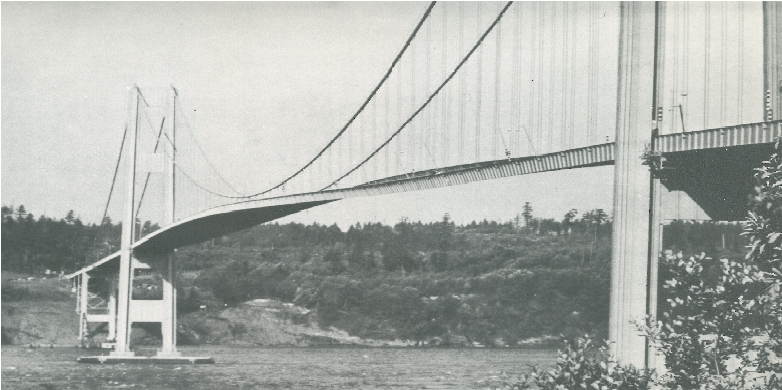
Figure 1. The collapsed Tacoma Narrows Bridge (1940).

one can see the roadway of the TNB under a torsional oscillation. This kind of oscillation was considered the main cause of the collapse [2, 31]. But the appearance of torsional oscillations is not an isolated event occurred only at the TNB. The Brighton Chain Pier was erected in 1823 and collapsed in 1836: Reid [28] reported valuable observations and sketched a picture illustrating the collapse see Figure 2

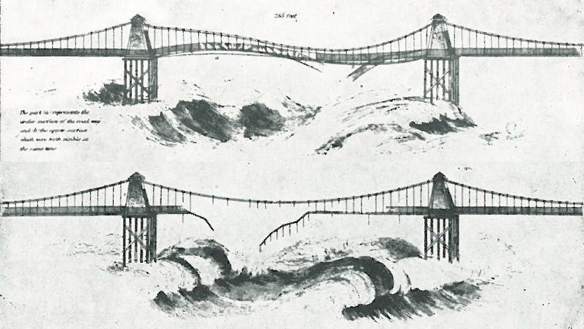
Figure 2. Collapse of the Brighton Chain Pier (1836).

(picture taken from [28]). The Wheeling Suspension Bridge was erected in West Virginia in 1849 and collapsed in a violent windstorm in 1854: according to [34], it twisted and writhed, and was dashed almost bottom upward. At last there seemed to be a determined twist along the entire span, about one half of the flooring being nearly reversed, and down went the immense structure from its dizzy height to the stream below, with an appalling crash and roar. Finally, let us mention that Irvine [19, Example 4.6, p.180] describes the collapse of the Matukituki Suspension Footbridge in New Zealand (occurred in 1977, just twelve days after completion) by writing that the deck persisted in lurching and twisting wildly until failure occurred, and for part of the time a node was noticeable at midspan. This description is completely similar to what can be seen in Figures 1 and 2 as well as in the video [33]. These are just few examples aiming to show that the very same instability was observed in several different bridges.

These accidents raised some fundamental questions of deep interest also for mathematicians. Longitudinal oscillations are to be expected in suspension bridges but

(Q1) why do longitudinal oscillations suddenly transform into torsional oscillations?

This question has drawn the attention of both mathematicians and engineers but, so far, no unanimously accepted response has been found. The distinguished civil and aeronautical engineer Robert Scanlan [29, p.209] attributes the appearance of torsional oscillations to some fortuitous condition. The word “fortuitous” highlights a lack of rigorous explanations and, according to [31], no real progress has been done in subsequent years.

The above collapses also show that the torsional oscillation has a particular shape, with a node at midspan. And it seems that this particular kind of torsional oscillation is the only one ever seen in suspension bridges. From the Official Report [2, p.31] we quote Prior to 10:00 A.M. on the day of the failure, there were no recorded instances of the oscillations being otherwise than the two cables in phase and with no torsional motions whereas from Smith-Vincent [32, p.21] we quote the only torsional mode which developed under wind action on the bridge or on the model is that with a single node at the center of the main span. This raises a further natural question:

(Q2) why do torsional oscillations appear with a node at midspan?

According to Eldridge [2, V-3], a witness on the day of the TNB collapse, the bridge appeared to be behaving in the customary manner and the motions were considerably less than had occurred many times before. From [2, p.20] we also learn that in the months prior to the collapse one principal mode of oscillation prevailed and that the modes of oscillation frequently changed. In particular, Farquharson [2, V-10] witnessed the collapse and wrote that the motions, which a moment before had involved a number of waves (nine or ten) had shifted almost instantly to two. This raises a third natural question:

(Q3) are there longitudinal oscillations which are more prone to generate torsional oscillations?

The purpose of this paper is to use the semilinear plate model developed in [16] and to adapt it to a suspension bridge having the same parameters as the collapsed TNB. By analyzing both theoretically and numerically this model, we will give an answer to the above questions (Q1), (Q2) and (Q3).

This paper is organized as follows. In Section 2 we recall and slightly modify the model introduced in [16], in particular we discuss the nonlinear restoring force due to the hangers+cables system. In Section 3 we study in great detail the oscillating modes of the plate, according to the TNB parameters. In Section 4 we analyze the full evolution equation in the case where the system is isolated: we obtain a fourth order hyperbolic equations and we show that the initial-boundary-value problem is well posed. Then we define what we mean by torsional stability and we state two sufficient conditions for the stability. In Section 5 we numerically compute the thresholds of stability, according to our definition. In Section 6 we validate our results from several points of view: we show that the linearization and the uncoupling procedures do not alter the results and that a full numerical analysis does not give significantly different responses. Sections 7 and 8 are devoted to the proofs of the stability results. Finally, in Section 9 we afford an answer to the above questions.

2. A nonlinear model for a dynamic suspension bridge

We follow the mathematical model suggested in [16] by modifying it in some aspects. We view the roadway (or deck) of a suspension bridge as a long narrow rectangular thin plate hinged at the two opposite short edges and free on the remaining two edges. Let $L$ denote its length and $2\ell$ denote its width; a realistic assumption is that $2\ell\cong\frac{L}{100}$. The rectangular plate $\Omega\subset{\mathbb{R}}^{2}$ is then

$$\Omega=(0,L)\times(-\ell,\ell)\,.$$

Let us first discuss different positions of the plate depending on the forces acting on it. If the plate had no mass (as a sheet of paper) and there were no loads acting on the plate, it would take the horizontal equilibrium position $u_{0}$, see Figure 3. If the plate was only subject to its own weight $w$ (dead load) it would take a $\cup$-position such as $u_{w}$ in Figure 3. If the plate had no weight but it was subject to the restoring force of the cables-hangers system, it would take a $\cap$-position such as $u_{h}$: this is also the position of the lower endpoints of the hangers before the roadway is installed. If both the weight and the action of the hangers are considered, the two effects cancel and the equilibrium position $u_{0}\equiv 0$ is recovered.

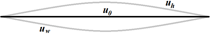
Figure 3. Different positions of the bridge.

Since the bending energy of the plate vanishes when it is in position $u_{0}\equiv 0$, the unknown function should be the displacement of the plate with respect to the equilibrium $u_{0}$. Augusti-Sepe [5] (see also [4]) view the restoring force at the endpoints of a cross-section of the roadway as composed by two connected springs, the top one representing the action of the sustaining cable and the bottom one (connected with the roadway) representing the hangers, see Figure 4.

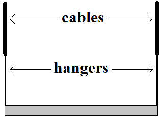
Figure 4. The cables+hangers system modeled with two connected springs.

The action of the cables is considered by Bartoli-Spinelli [6, p.180] the main cause of the nonlinearity of the restoring force: they suggest quadratic and cubic perturbations of a linear behavior. If $u$ denotes the downwards displacement of the deck, here we simply take

(1) $$g(u)=k_{1}\,u+k_{2}\,u^{3}$$

for some $k_{1},k_{2}>0$ depending on the elasticity of the cables and hangers. Let us mention that Plaut-Davis [27, $\S$ 3.5] make the same choice.

The action of the hangers on the roadway is confined in the union of two thin strips parallel and adjacent to the two long edges of the plate $\Omega$, that is, in a set of the type

(2) $$\omega:=(0,L)\times[(-\ell,-\ell+\varepsilon)\cup(\ell-\varepsilon,\ell)]$$

with $\varepsilon>0$ small compared to $\ell$. Summarizing, we take as restoring force and potential due to the cables-hangers system

(3) $$h(y,u)=\Upsilon(y)\,\Big{(}k_{1}\,u+k_{2}\,u^{3}\Big{)}\,,\qquad H(y,u)=\int_{0}^{u}h(y,\tau)d\tau=\Upsilon(y)\,\left(\frac{k_{1}}{2}\,u^{2}+\frac{k_{2}}{4}\,u^{4}\right)\,,$$

where $\Upsilon$ is the characteristic function of $(-\ell,-\ell+\varepsilon)\cup(\ell-\varepsilon,\ell)$.

The derivation of the bending energy of an elastic plate goes back to Kirchhoff [22] and Love [24], see also [16] for a synthesized form. The total static energy of the bridge is obtained by adding the potential energy from (3) to the bending energy of the plate:

(4) $$\mathbb{E}_{T}(u)=\frac{E\,d^{3}}{12(1-\sigma^{2})}\int_{\Omega}\left(\frac{1}{2}\left(\Delta u\right)^{2}+(\sigma-1)\det(D^{2}u)\right)+\int_{\Omega}\big{(}H(y,u)-fu\big{)}$$

where $f$ is an external force, $d$ denotes the thickness of the plate, $E$ is the Young modulus and $\sigma$ is the Poisson ratio. For a plate, the Poisson ratio is the negative ratio of transverse to axial strain: when a material is compressed in one direction, it tends to expand in the other two directions. The Poisson ratio $\sigma$ is a measure of this effect, it is the fraction of expansion divided by the fraction of compression for small values of these changes. Usually one has

(5) $$0<\sigma<\frac{1}{2}\,.$$

A functional space where the energy $\mathbb{E}_{T}$ is well-defined is

$$H^{2}_{*}(\Omega):=\Big{\{}w\in H^{2}(\Omega);\,w=0\mbox{ on }\{0,L\}\times(-\ell,\ell)\Big{\}}$$

which is a Hilbert space when endowed with the scalar product

(6) $$(u,v)_{H^{2}_{*}}:=\int_{\Omega}\left[\Delta u\Delta v+(1-\sigma)(2u_{xy}v_{xy}-u_{xx}v_{yy}-u_{yy}v_{xx})\right]\,dxdy\,,$$

see [16, Lemma 4.1]. We also consider

$$\mathcal{H}(\Omega):=\mbox{ the dual space of }H^{2}_{*}(\Omega)$$

and we denote by $\langle\cdot,\cdot\rangle$ the corresponding duality. Since we are in the plane, $H^{2}(\Omega)\subset C^{0}(\overline{\Omega})$ so that the condition on $\{0,L\}\times(-\ell,\ell)$ introduced in the definition of $H^{2}_{*}(\Omega)$ is satisfied pointwise. If $f\in L^{1}(\Omega)$ then the functional $\mathbb{E}_{T}$ is well-defined in $H^{2}_{*}(\Omega)$, while if $f\in\mathcal{H}(\Omega)$ we need to replace $\int_{\Omega}fu$ with $\langle f,u\rangle$ although we will not mention this in the sequel.

If the load also depends on time, $f=f(x,y,t)$, and if $m$ denotes the mass density of the plate, then the kinetic energy of the plate should be added to the static energy (4):

(7) $${\mathcal{E}_{u}}(t):=\frac{m}{2}\int_{\Omega}u_{t}^{2}+\frac{E\,d^{3}}{12(1-\sigma^{2})}\int_{\Omega}\left(\frac{(\Delta u)^{2}}{2}+(\sigma-1)\det(D^{2}u)\right)+\int_{\Omega}\big{(}H(y,u)-fu\big{)}\,.$$

This is the total energy of a nonlinear dynamic bridge. As for the action, one has to take the difference between kinetic energy and potential energy and integrate over an interval of time $[0,T]$:

$$\mathcal{A}(u):=\int_{0}^{T}\left[\frac{m}{2}\int_{\Omega}u_{t}^{2}-\frac{E\,d^{3}}{12(1-\sigma^{2})}\int_{\Omega}\left(\frac{(\Delta u)^{2}}{2}+(\sigma-1)\det(D^{2}u)\right)-\int_{\Omega}\big{(}H(y,u)-fu\big{)}\right]\,dt\,.$$

The equation of the motion of the bridge is obtained by taking the critical points of the functional $\mathcal{A}$:

$$m\,u_{tt}+\frac{E\,d^{3}}{12(1-\sigma^{2})}\,\Delta^{2}u+h(y,u)=f\qquad\text{in }\Omega\times(0,T)\,.$$

Due to internal friction, we add a damping term and obtain

(8) $$\left\{\begin{array}[]{ll}\!\!mu_{tt}\!+\!\delta u_{t}\!+\!\frac{E\,d^{3}}{12(1-\sigma^{2})}\Delta^{2}u\!+\!h(y,u)\!=\!f&\text{in }\Omega\!\times\!(0,T)\\ \!\!u(0,y,t)\!=\!u_{xx}(0,y,t)\!=\!u(L,y,t)\!=\!u_{xx}(L,y,t)\!=\!0&\text{for }(y,t)\!\in\!(-\ell,\ell)\!\times\!(0,T)\\ \!\!u_{yy}(x,\pm\ell,t)\!+\!\sigma u_{xx}(x,\pm\ell,t)\!=\!0&\text{for }(x,t)\!\in\!(0,L)\!\times\!(0,T)\\ \!\!u_{yyy}(x,\pm\ell,t)\!+\!(2-\sigma)u_{xxy}(x,\pm\ell,t)\!=\!0&\text{for }(x,t)\!\in\!(0,L)\!\times\!(0,T)\\ \!\!u(x,y,0)\!=\!u_{0}(x,y)\,,\quad u_{t}(x,y,0)\!=\!u_{1}(x,y)&\text{for }(x,y)\!\in\!\Omega\end{array}\right.$$

where $\delta$ is a positive constant. We refer to [16] for the derivation of the boundary conditions.

For a different model of suspension bridges, similar to the one considered in [3], Irvine [19, p.176] ignores damping of both structural and aerodynamic origin. His purpose is to simplify as much as possible the model by maintaining its essence, that is, the conceptual design of bridges. Here we follow this suggestion and consider the isolated version of (8) for which global existence is expected ($T=\infty$). This isolated version of (8) reads

(9) $$mw_{tt}\!+\!\frac{E\,d^{3}}{12(1-\sigma^{2})}\Delta^{2}w\!+\!\Upsilon(y)(k_{1}w+k_{2}w^{3})\!=\!0\qquad\text{for }(x,y)\in(0,L)\times\left(-\ell,\ell\right),\,t>0\,,$$

where $w$ denotes the downwards vertical displacement and all the constants are defined in Section 2.

In order to set up a reliable model, we consider the lengths of the plate as in the collapsed TNB. According to [2, p.11], we have

(10) $$L=2800\,\mbox{ft.}\approx 853.44\,m\,,\quad 2\ell=39\,\mbox{ft.}\approx 11.89\,m\,,\qquad\mbox{that is,}\qquad\frac{2\ell}{L}=\frac{39}{2800}\approx\frac{1}{75}=\frac{\,\frac{2\pi}{150}\,}{\pi}\,.$$

Therefore, we may scale the plate $(0,L)\times(-\ell,\ell)$ to $(0,\pi)\times(-\tfrac{\pi}{150},\tfrac{\pi}{150})$. Then we take the amplitude of the strip $\omega$ (see (2)) containing the hangers also as at the TNB, see [2, p.11]:

(11) $$\varepsilon=\frac{\pi}{1500}\,.$$

Referring to Section 5 for the values of the involved parameters, we put

(12) $$w(x,y,t)=\sqrt{\frac{k_{1}}{k_{2}}}\ u\left(\frac{\pi x}{L},\frac{\pi y}{L},\sqrt{\frac{k_{1}}{m}}\,t\right)\qquad\mbox{and}\qquad\gamma=\frac{E\,d^{3}}{12k_{1}(1-\sigma^{2})}\,\frac{\pi^{4}}{L^{4}}\,.$$

Then (9) becomes an equation where the only parameter is the coefficient of the biharmonic term:

$$u_{tt}+\gamma\,\Delta^{2}u+\Upsilon(y)(u+u^{3})=0\qquad\text{in }(0,\pi)\times\left(-\frac{\pi}{150},\frac{\pi}{150}\right)\times{\mathbb{R}}_{+}$$

and $\Upsilon$ is the characteristic function of the set $(-\frac{\pi}{150},-\frac{3\pi}{500})\cup(\frac{3\pi}{500},\frac{\pi}{150})$. Finally, we notice that for metals the value of $\sigma$ lies around $0.3$, see [24, p.105], while for concrete we have $0.1<\sigma<0.2$. Since the suspended structure of the TNB consisted of a “mixture” of concrete and metal (see [2, p.13]), we take

(13) $$\sigma=0.2\,.$$

Then by using (12) we find the dimensionless version of the problem under study

(14) $$\left\{\begin{array}[]{ll}\!\!u_{tt}\!+\!\gamma\Delta^{2}u\!+\!\Upsilon(y)(u+u^{3})\!=\!0&\text{in }\Omega\!\times\!(0,\infty)\\ \!\!u(0,y,t)\!=\!u_{xx}(0,y,t)\!=\!u(\pi,y,t)\!=\!u_{xx}(\pi,y,t)\!=\!0&\text{for }(y,t)\!\in\!(-\frac{\pi}{150},\frac{\pi}{150})\!\times\!(0,\infty)\\ \!\!u_{yy}(x,\pm\frac{\pi}{150},t)\!+\!0.2\cdot u_{xx}(x,\pm\frac{\pi}{150},t)\!=\!0&\text{for }(x,t)\!\in\!(0,\pi)\!\times\!(0,\infty)\\ \!\!u_{yyy}(x,\pm\frac{\pi}{150},t)\!+\!1.8\cdot u_{xxy}(x,\pm\frac{\pi}{150},t)\!=\!0&\text{for }(x,t)\!\in\!(0,\pi)\!\times\!(0,\infty)\\ \!\!u(x,y,0)\!=\!u_{0}(x,y)\,,\quad u_{t}(x,y,0)\!=\!u_{1}(x,y)&\text{for }(x,y)\!\in\!\Omega\end{array}\right.$$

where $\Omega=(0,\pi)\times(-\frac{\pi}{150},\frac{\pi}{150})$. The initial-boundary value problem (14) is isolated, which means that it has a conserved quantity. This quantity is the energy introduced in (7) which is constant in time:

(15) $$E(u)=\int_{\Omega}\frac{1}{2}u_{t}^{2}\,dxdy+\int_{\Omega}\left(\frac{\gamma}{2}(\Delta u)^{2}+\frac{4\gamma}{5}(u_{xy}^{2}-u_{xx}u_{yy})+\Upsilon(y)\,\left(\frac{u^{2}}{2}+\frac{u^{4}}{4}\right)\right)\,dxdy\,.$$

3. The eigenfunctions of the linearized problem

For the rectangular plate $\Omega=(0,\pi)\times(-\ell,\ell)$ with Poisson ratio $\sigma$ we are interested in the eigenfunctions of the eigenvalue problem

(16) $$\begin{cases}\Delta^{2}w=\lambda w&\qquad\text{in }\Omega\\ w(0,y)=w_{xx}(0,y)=w(\pi,y)=w_{xx}(\pi,y)=0&\qquad\text{for }y\in(-\ell,\ell)\\ w_{yy}(x,\pm\ell)+\sigma w_{xx}(x,\pm\ell)=w_{yyy}(x,\pm\ell)+(2-\sigma)w_{xxy}(x,\pm\ell)=0&\qquad\text{for }x\in(0,\pi)\,.\end{cases}$$

Problem (16) admits the following variational formulation: a nontrivial function $w\in H^{2}_{*}(\Omega)$ is an eigenfunction of (16) if there exists $\lambda\in{\mathbb{R}}$ (an eigenvalue) such that

$$\int_{\Omega}\left[\Delta w\Delta v+(1-\sigma)(2w_{xy}v_{xy}-w_{xx}v_{yy}-w_{yy}v_{xx})-\lambda wv\right]\,dxdy=0\qquad\text{for all }v\in H^{2}_{*}(\Omega)\,.$$

We recall from [16, Theorem 7.6] a statement describing the whole spectrum and characterizing the eigenfunctions. It is shown there that the eigenfunctions may have one of the following forms:

Proposition 3.1.

Assume (5). Then the set of eigenvalues of (16) may be ordered in an increasing sequence $\{\lambda_{k}\}$ of strictly positive numbers diverging to $+\infty$ and any eigenfunction belongs to $C^{\infty}(\overline{\Omega})$; the set of eigenfunctions of (16) is a complete system in $H^{2}_{*}(\Omega)$. Moreover:

$(i)$ for any $m\geqslant 1$, there exists a unique eigenvalue $\lambda=\mu_{m,1}\in((1-\sigma)^{2}m^{4},m^{4})$ with corresponding eigenfunction

$$\left[\big{[}\mu_{m,1}^{1/2}-(1-\sigma)m^{2}\big{]}\,\tfrac{\cosh\Big{(}y\sqrt{m^{2}+\mu_{m,1}^{1/2}}\Big{)}}{\cosh\Big{(}\ell\sqrt{m^{2}+\mu_{m,1}^{1/2}}\Big{)}}+\big{[}\mu_{m,1}^{1/2}+(1-\sigma)m^{2}\big{]}\,\tfrac{\cosh\Big{(}y\sqrt{m^{2}-\mu_{m,1}^{1/2}}\Big{)}}{\cosh\Big{(}\ell\sqrt{m^{2}-\mu_{m,1}^{1/2}}\Big{)}}\right]\sin(mx)\,;$$

$(ii)$ for any $m\geqslant 1$, there exist infinitely many eigenvalues $\lambda=\mu_{m,k}>m^{4}$ ($k\geqslant 2$) with corresponding eigenfunctions

$$\left[\big{[}\mu_{m,k}^{1/2}-(1-\sigma)m^{2}\big{]}\,\tfrac{\cosh\Big{(}y\sqrt{\mu_{m,k}^{1/2}+m^{2}}\Big{)}}{\cosh\Big{(}\ell\sqrt{\mu_{m,k}^{1/2}+m^{2}}\Big{)}}+\big{[}\mu_{m,k}^{1/2}+(1-\sigma)m^{2}\big{]}\,\tfrac{\cos\Big{(}y\sqrt{\mu_{m,k}^{1/2}-m^{2}}\Big{)}}{\cos\Big{(}\ell\sqrt{\mu_{m,k}^{1/2}-m^{2}}\Big{)}}\right]\sin(mx)\,;$$

$(iii)$ for any $m\geqslant 1$, there exist infinitely many eigenvalues $\lambda=\nu_{m,k}>m^{4}$ ($k\geqslant 2$) with corresponding eigenfunctions

$$\left[\big{[}\nu_{m,k}^{1/2}-(1-\sigma)m^{2}\big{]}\,\tfrac{\sinh\Big{(}y\sqrt{\nu_{m,k}^{1/2}+m^{2}}\Big{)}}{\sinh\Big{(}\ell\sqrt{\nu_{m,k}^{1/2}+m^{2}}\Big{)}}+\big{[}\nu_{m,k}^{1/2}+(1-\sigma)m^{2}\big{]}\,\tfrac{\sin\Big{(}y\sqrt{\nu_{m,k}^{1/2}-m^{2}}\Big{)}}{\sin\Big{(}\ell\sqrt{\nu_{m,k}^{1/2}-m^{2}}\Big{)}}\right]\sin(mx)\,;$$

$(iv)$ for any $m\geqslant 1$ satisfying $\ell m\sqrt{2}\,\coth(\ell m\sqrt{2})>\left(\frac{2-\sigma}{\sigma}\right)^{2}$ there exists an eigenvalue $\lambda=\nu_{m,1}\in(\mu_{m,1},m^{4})$ with corresponding eigenfunction

$$\left[\big{[}\nu_{m,1}^{1/2}-(1-\sigma)m^{2}\big{]}\,\tfrac{\sinh\Big{(}y\sqrt{m^{2}+\nu_{m,1}^{1/2}}\Big{)}}{\sinh\Big{(}\ell\sqrt{m^{2}+\nu_{m,1}^{1/2}}\Big{)}}+\big{[}\nu_{m,1}^{1/2}+(1-\sigma)m^{2}\big{]}\,\tfrac{\sinh\Big{(}y\sqrt{m^{2}-\nu_{m,1}^{1/2}}\Big{)}}{\sinh\Big{(}\ell\sqrt{m^{2}-\nu_{m,1}^{1/2}}\Big{)}}\right]\sin(mx)\,.$$

Finally, if the unique positive solution $s>0$ of the equation

(17) $$\tanh(\sqrt{2}s\ell)=\left(\frac{\sigma}{2-\sigma}\right)^{2}\,\sqrt{2}s\ell$$

is not an integer, then the only eigenvalues and eigenfunctions are the ones given in $(i)-(iv)$.

Of course, (17) has probability 0 to occur in a real bridge; if it occurs, there is an additional eigenvalue and eigenfunction, see [16]. The eigenvalues $\lambda_{k}$ are solutions of explicit equations. More precisely:

$(i)$ the eigenvalue $\lambda=\mu_{m,1}$ is the unique value $\lambda\in((1-\sigma)^{2}m^{4},m^{4})$ such that

$$\sqrt{m^{2}\!-\!\lambda^{1/2}}\big{(}\lambda^{1/2}\!+\!(1\!-\!\sigma)m^{2}\big{)}^{2}\tanh(\ell\sqrt{m^{2}\!-\!\lambda^{1/2}})\!=\!\sqrt{m^{2}\!+\!\lambda^{1/2}}\big{(}\lambda^{1/2}\!-\!(1\!-\!\sigma)m^{2}\big{)}^{2}\tanh(\ell\sqrt{m^{2}\!+\!\lambda^{1/2}})\,;$$

$(ii)$ the eigenvalues $\lambda=\mu_{m,k}$ ($k\geqslant 2$) are the solutions $\lambda>m^{4}$ of the equation

$$\sqrt{\lambda^{1/2}\!-\!m^{2}}\big{(}\lambda^{1/2}\!+\!(1\!-\!\sigma)m^{2}\big{)}^{2}\tan(\ell\sqrt{\lambda^{1/2}\!-\!m^{2}})\!=\!-\!\sqrt{\lambda^{1/2}\!+\!m^{2}}\big{(}\lambda^{1/2}\!-\!(1\!-\!\sigma)m^{2}\big{)}^{2}\tanh(\ell\sqrt{\lambda^{1/2}\!+\!m^{2}})\,;$$

$(iii)$ the eigenvalues $\lambda=\nu_{m,k}$ ($k\geqslant 2$) are the solutions $\lambda>m^{4}$ of the equation

$$\sqrt{\lambda^{1/2}\!-\!m^{2}}\big{(}\lambda^{1/2}\!+\!(1\!-\!\sigma)m^{2}\big{)}^{2}\tanh(\ell\sqrt{\lambda^{1/2}\!+\!m^{2}})\!=\!\sqrt{\lambda^{1/2}\!+\!m^{2}}\big{(}\lambda^{1/2}\!-\!(1\!-\!\sigma)m^{2}\big{)}^{2}\tan(\ell\sqrt{\lambda^{1/2}\!-\!m^{2}})\,;$$

$(iv)$ the eigenvalue $\lambda=\nu_{m,1}$ is the unique value $\lambda\in((1-\sigma)^{2}m^{4},m^{4})$ such that

$$\sqrt{m^{2}\!-\!\lambda^{1/2}}\big{(}\lambda^{1/2}\!+\!(1\!-\!\sigma)m^{2}\big{)}^{2}\tanh(\ell\sqrt{\lambda^{1/2}\!+\!m^{2}})\!=\!\sqrt{\lambda^{1/2}\!+\!m^{2}}\big{(}\lambda^{1/2}\!-\!(1\!-\!\sigma)m^{2}\big{)}^{2}\tanh(\ell\sqrt{\lambda^{1/2}\!-\!m^{2}})\,.$$

The least eigenvalue is $\lambda_{1}=\mu_{1,1}$: the corresponding eigenfunction is of one sign over $\Omega$ and this fact is by far nontrivial. It is well-known that the first eigenfunction of some biharmonic problems may change sign. When $\Omega$ is a square, Coffman [15] proved that the first eigenfunction of the clamped plate problem changes sign, see also [21] for more general results. Moreover, Knightly-Sather [20, Section 3] show that the buckling eigenvalue problem for a fully hinged (simply supported) rectangular plate, that is with $u=\Delta u=0$ on the four edges, may admit a least eigenvalue of multiplicity 2. Hence, the positivity of the first eigenfunction of (16) is not for free. Due to the $L^{2}$-orthogonality of eigenfunctions, it is the only positive eigenfunction of (16).

The eigenfunctions in $(i)-(ii)$ are even with respect to $y$ whereas the eigenfunctions in $(iii)-(iv)$ are odd. We call longitudinal eigenfunctions the eigenfunctions of the kind $(i)-(ii)$ and torsional eigenfunctions the eigenfunctions of the kind $(iii)-(iv)$. Since $\ell$ is small, the former are essentially of the kind $c_{m}\sin(mx)$ whereas the latter are of the kind $c_{m}y\sin(mx)$. The pictures in Figure 5 display the first two longitudinal eigenfunctions (approximately described by $c_{1}\sin(x)$ and $c_{2}\sin(2x)$) and the second torsional eigenfunction (approximately described by $c_{2}y\sin(2x)$). In each picture the displacement of the roadway is compared with equilibrium.

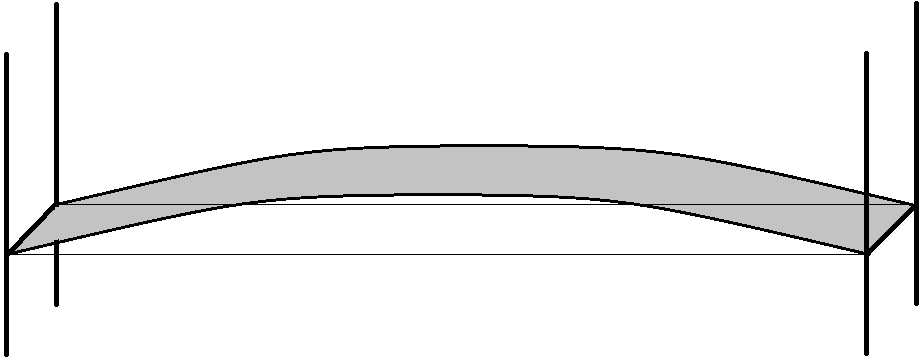
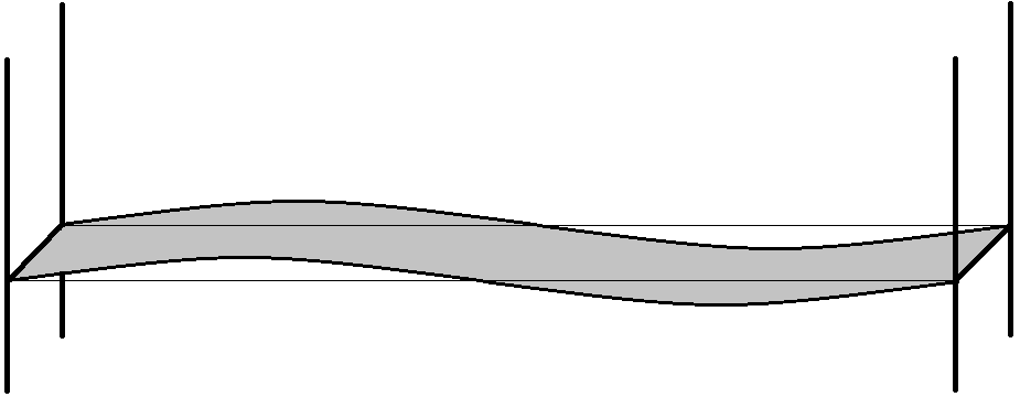
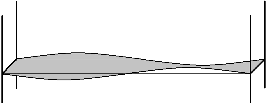
Figure 5. Some possible oscillations of a bridge roadway.

Of particular interest is the lower picture in Figure 5 which corresponds to a torsional eigenfunction with a node at midspan. This is precisely the behavior of the TNB prior to its collapse in November 1940, see the video [33] and Figure 1. This is also the behavior of the Brighton Chain Pier, see Figure 2, and of the other bridges described in the introduction. With the notations of Proposition 3.1, this common behavior of suspension bridges may be rephrased as follows

(18) $$\begin{array}[]{ccc}\mbox{the oscillations causing the collapse of a suspension bridge}\\ \mbox{are of the kind $c_{2}y\sin(2x)$, as represented in the bottom picture of Figure \ref{kable},}\\ \mbox{and correspond to the eigenvalue $\nu_{2,2}$, as given by Proposition \ref{eigenvalue}.}\end{array}$$

We remark that the eigenfunction corresponding to the eigenvalue $\nu_{1,1}$ is of the kind $c_{2}y\sin(x)$ but this eigenvalue in general does not exist since the inequality in Proposition 3.1 $(iv)$ is usually satisfied only for large $m$.

By (10) we may take

(19) $$\ell=\frac{\pi}{150}\,.$$

With the choices in (13) and (19) we numerically obtained the eigenvalues of (16) as reported in Table 1. We only quote the least 16 eigenvalues because we are mainly interested in the second torsional eigenvalue which is, precisely, the 16th.

eigenvalue	$\lambda_{1}$	$\lambda_{2}$	$\lambda_{3}$	$\lambda_{4}$	$\lambda_{5}$	$\lambda_{6}$	$\lambda_{7}$	$\lambda_{8}$
kind	$\mu_{1,1}$	$\mu_{2,1}$	$\mu_{3,1}$	$\mu_{4,1}$	$\mu_{5,1}$	$\mu_{6,1}$	$\mu_{7,1}$	$\mu_{8,1}$
$\sqrt{\rm{eigenvalue}}\approx$	$0.98$	$3.92$	$8.82$	$15.68$	$24.5$	$35.28$	$48.02$	$62.73$

eigenvalue	$\lambda_{9}$	$\lambda_{10}$	$\lambda_{11}$	$\lambda_{12}$	$\lambda_{13}$	$\lambda_{14}$	$\lambda_{15}$	$\lambda_{16}$
kind	$\mu_{9,1}$	$\mu_{10,1}$	$\nu_{1,2}$	$\mu_{11,1}$	$\mu_{12,1}$	$\mu_{13,1}$	$\mu_{14,1}$	$\nu_{2,2}$
$\sqrt{\rm{eigenvalue}}\approx$	$79.39$	$98.03$	$104.61$	$118.62$	$141.19$	$165.72$	$192.21$	$209.25$

Table 1. Approximate value of the least 16 eigenvalues of (16) for $\sigma=0.2$ and $\ell=\frac{\pi}{150}$.

Our results are obtained with the parameters of the TNB, see (10), (13) and (19). As already mentioned in the introduction, Farquharson [2, V-10] witnessed the collapse and wrote that the motions, which a moment before had involved a number of waves (nine or ten) had shifted almost instantly to two. Note that the longitudinal eigenvalue immediately preceding the least torsional eigenvalue is $\mu_{10,1}$: it involves the function $\sin(10x)$ which has precisely “ten waves”. This explains why at the TNB the torsional instability occurred when the bridge was longitudinally oscillating like $\sin(10x)$. Then, if no constraint acts on the deck, the energy should transfer to the eigenfunction corresponding to $\nu_{1,2}$ which has a behavior like $y\sin(x)$. Among longitudinal eigenfunctions, the tenth is the most prone to torsional instability since the ratio between torsional eigenvalues and longitudinal eigenvalues is minimal (close to 1) precisely for the tenth longitudinal eigenfunction: why small ratios yield strong instability is explained for a simplified model through Mathieu equations in [9]. However, in the case of a bridge, the sustaining cable yields a serious constraint. With a rude approximation, the cables may be considered as inextensible. A better point of view is that they are only “weakly extensible”, which means that their elongation cannot bee too large. In Figure 6

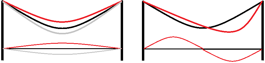
Figure 6. Elongation of the cable generated by the oscillations of the deck.

we represent the deformation of a cable in the two situations where the deck behaves like $\sin(x)$ and like $\sin(2x)$. It turns out that the no-noded behavior $\sin(x)$ (on the left) only allows small vertical displacements of the deck (between the grey and red positions) and, therefore, small torsional oscillations of the kind $y\sin(x)$. This is confirmed by numerical experiments for models where the cable plays a dominant role, see [10] where it is shown that, basically, “the first mode does not exist” in actual bridges. On the contrary, the one-noded behavior $\sin(2x)$ allows much larger torsional oscillations of the kind $y\sin(2x)$, see the right picture. Our explanation of the transition described by Farquharson is that when the oscillation $\sin(10x)$ became sufficiently large, reaching the threshold of the torsional instability, the cable forced the transition to the eigenfunction $y\sin(2x)$ instead of $y\sin(x)$. This gives a sound explanation to (18) and a first answer to (Q2), see Section 5.

If we slightly modify the choices in (13) and (19), still in the range of the TNB, we obtain the eigenvalues of (16) as reported in Table 2.

eigenvalue	$\lambda_{1}$	$\lambda_{2}$	$\lambda_{3}$	$\lambda_{4}$	$\lambda_{5}$	$\lambda_{6}$	$\lambda_{7}$	$\lambda_{8}$
kind	$\mu_{1,1}$	$\mu_{2,1}$	$\mu_{3,1}$	$\mu_{4,1}$	$\mu_{5,1}$	$\mu_{6,1}$	$\mu_{7,1}$	$\mu_{8,1}$
$\sqrt{\rm{eigenvalue}}\approx$	$0.97$	$3.87$	$8.71$	$15.49$	$24.21$	$34.87$	$47.46$	$62$

eigenvalue	$\lambda_{9}$	$\lambda_{10}$	$\lambda_{11}$	$\lambda_{12}$	$\lambda_{13}$	$\lambda_{14}$	$\lambda_{15}$	$\lambda_{16}$
kind	$\mu_{9,1}$	$\mu_{10,1}$	$\nu_{1,2}$	$\mu_{11,1}$	$\mu_{12,1}$	$\mu_{13,1}$	$\mu_{14,1}$	$\nu_{2,2}$
$\sqrt{\rm{eigenvalue}}\approx$	$78.48$	$96.9$	$97.24$	$117.27$	$139.58$	$163.84$	$190.1$	$194.51$

Table 2. Approximate value of the least 16 eigenvalues of (16) for $\sigma=0.25$ and $\ell=\frac{\pi}{144}$.

While comparing with Table 1, it is noticeable that all the eigenvalues have slightly lowered but the qualitative behavior and the corresponding explanation remain the same.

4. Torsional stability of the longitudinal modes

4.1. Existence, uniqueness, and finite dimensional approximation of the solution

Let $\Upsilon$ be the characteristic function of the set $(-\frac{\pi}{150},-\frac{3\pi}{500})\cup(\frac{3\pi}{500},\frac{\pi}{150})$ and let

(20) $$h(y,u)=\Upsilon(y)\,\Big{(}u+u^{3}\Big{)}\,.$$

We say that

(21) $$u\in C^{0}({\mathbb{R}}_{+};H^{2}_{*}(\Omega))\cap C^{1}({\mathbb{R}}_{+};L^{2}(\Omega))\cap C^{2}({\mathbb{R}}_{+};\mathcal{H}(\Omega))$$

is a solution of (14) if it satisfies the initial conditions and if

(22) $$\langle u^{\prime\prime}(t),v\rangle+\gamma(u(t),v)_{H^{2}_{*}}+(h(y,u(t)),v)_{L^{2}}=0\qquad\forall v\in H^{2}_{*}(\Omega)\,,\ \forall t\in(0,T)\,,$$

see (6). Then, by arguing as in [16, Theorem 3.6] we may prove the following result.

Theorem 4.1.

Assume (5). Let $u_{0}\in H^{2}_{*}(\Omega)$ and $u_{1}\in L^{2}(\Omega)$. Then there exists a unique solution $u=u(t)$ of (14) and its energy (15) satisfies

$$E(u(t))\equiv\int_{\Omega}\frac{1}{2}u_{1}^{2}\,dxdy+\int_{\Omega}\left(\frac{\gamma}{2}(\Delta u_{0})^{2}+\frac{4\gamma}{5}((u_{0})_{xy}^{2}-(u_{0})_{xx}(u_{0})_{yy})+\Upsilon(y)\,\left(\frac{u_{0}^{2}}{2}+\frac{u_{0}^{4}}{4}\right)\right)\,dxdy\,.$$

Sketch of the proof of Theorem 4.1. The proof of Theorem 4.1 makes use of a Galerkin method. The solution of (14) is the limit (in a suitable topology) of a sequence of solutions of approximated problems in finite dimensional spaces. By Proposition 3.1 we may consider an orthogonal complete system $\{w_{k}\}_{k\geqslant 1}\subset H^{2}_{*}(\Omega)$ of eigenfunctions of (16) such that $\|w_{k}\|_{L^{2}}=1$. Let $\{\lambda_{k}\}_{k\geqslant 1}$ be the corresponding eigenvalues and, for any $m\geqslant 1$, put $W_{m}:={\rm span}\{w_{1},\dots,w_{m}\}$. For any $m\geqslant 1$ let

$$u_{0}^{m}:=\sum_{i=1}^{m}(u_{0},w_{i})_{L^{2}}w_{i}=\sum_{i=1}^{m}\lambda_{i}^{-1}(u_{0},w_{i})_{H^{2}_{*}}\,w_{i}\ \mbox{ and }\ u_{1}^{m}=\sum_{i=1}^{m}(u_{1},w_{i})_{L^{2}}\,w_{i}$$

so that $u_{0}^{m}\to u_{0}$ in $H^{2}_{*}(\Omega)$ and $u_{1}^{m}\to u_{1}$ in $L^{2}(\Omega)$ as $m\to+\infty$. Fix $T>0$; for any $m\geqslant 1$ one seeks a solution $u_{m}\in C^{2}([0,T];W_{m})$ of the variational problem

(23) $$\begin{cases}(u^{\prime\prime}(t),v)_{L^{2}}+\gamma(u(t),v)_{H^{2}_{*}}+(h(y,u(t)),v)_{L^{2}}=0\\ u(0)=u_{0}^{m}\,,\quad u^{\prime}(0)=u_{1}^{m}\end{cases}$$

for any $v\in W_{m}$ and $t\in(0,T)$. If we put

(24) $$u_{m}(t)=\sum_{i=1}^{m}g_{i}^{m}(t)w_{i}\qquad\mbox{and}\qquad g^{m}(t):=(g_{1}^{m}(t),\dots,g_{m}^{m}(t))^{T}$$

then the vector valued function $g^{m}$ solves

(25) $$\begin{cases}(g^{m}(t))^{\prime\prime}+\gamma\,\Lambda_{m}g^{m}(t)+\Phi_{m}(g^{m}(t))=0\qquad\forall t\in(0,T)\\ g^{m}(0)=((u_{0},w_{1})_{L^{2}},\dots,(u_{0},w_{m})_{L^{2}})^{T}\,,\quad(g^{m})^{\prime}(0)=((u_{1},w_{1})_{L^{2}},\dots,(u_{1},w_{m})_{L^{2}})^{T}\end{cases}$$

where $\Lambda_{m}:={\rm diag}(\lambda_{1},\dots,\lambda_{m})$ and $\Phi_{m}:{\mathbb{R}}^{m}\to{\mathbb{R}}^{m}$ is the map defined by

$$\Phi_{m}(\xi_{1},\dots,\xi_{m}):=\left(\Big{(}h\Big{(}y,\sum_{j=1}^{m}\xi_{j}w_{j}\Big{)},w_{1}\Big{)}_{L^{2}},\dots,\Big{(}h\Big{(}y,\sum_{j=1}^{m}\xi_{j}w_{j}\Big{)},w_{m}\Big{)}_{L^{2}}\right)^{T}\,.$$

From (20) we deduce that $\Phi_{m}\in{\rm Lip_{loc}}({\mathbb{R}}^{m};{\mathbb{R}}^{m})$ and hence (25) admits a unique solution. Whence, the function $u_{m}(t)$ in (24) belongs $C^{2}([0,T);H^{2}_{*}(\Omega))$ and is a solution of the problem

(26) $$\begin{cases}u_{m}^{\prime\prime}(t)+\gamma\,Lu_{m}(t)+P_{m}(h(y,u_{m}(t)))=0\qquad\text{for any }t\geqslant 0\\ u_{m}(0)=u_{0}^{m}\,,\quad u_{m}^{\prime}(0)=u_{1}^{m}\end{cases}$$

where $L:H^{2}_{*}(\Omega)\to\mathcal{H}(\Omega)$ is implicitly defined by $\langle Lu,v\rangle:=(u,v)_{H^{2}_{*}}$ for any $u,v\in H^{2}_{*}(\Omega)$, and $P_{m}$ is the orthogonal projection from $H^{2}_{*}(\Omega)$ onto $W_{m}$. By arguing as in [16], one finds that the sequence $\{u_{m}\}$ converges in $C^{0}([0,T];H^{2}_{*}(\Omega))\cap C^{1}([0,T];L^{2}(\Omega))$ to a solution of (14).  $\Box$

The above proof shows that the solution of (14) may be obtained as the limit of a finite dimensional analysis performed with a finite number of modes. Let us fix some value $E>0$ for (15). Depending on the value of $E$, higher modes may be dropped, see [8, Section 3.3] for a detailed physical motivation and for some quantitative estimates. Our purpose is to study the torsional stability of the low modes in a sense that will be made precise in next section. In particular, the results obtained in Section 3 suggest to focus the attention on the lowest $16$ modes, including the two least torsional modes.

4.2. A theoretical characterization of torsional stability

In this section we give a precise definition of torsional stability. We point out that this might not be the only possible definition. However, the numerical results reported in Sections 5 and 6 show that our characterization well describes the instability.

We take again $h(y,u)$ as in (20) and we fix $m=16$ which is the position of the second torsional mode. From Proposition 3.1 and Table 1 we know that the eigenvalues and the $L^{2}$-normalized eigenfunctions up to the 16th are given by

$$\lambda_{k}=\left\{\begin{array}[]{llll}\!\!\mu_{k,1}&\text{if }1\leqslant k\leqslant 10\\ \!\!\nu_{1,2}&\text{if }k=11\\ \!\!\mu_{k-1,1}&\text{if }12\leqslant k\leqslant 15\\ \!\!\nu_{2,2}&\text{if }k=16\end{array}\right.\qquad\qquad w_{k}(x,y)=\left\{\begin{array}[]{llll}\!\!\tfrac{v_{k}(y)\sin(kx)}{\omega_{k}}&\mbox{if }1\leqslant k\leqslant 10\\ \!\!\tfrac{\theta_{1}(y)\sin(x)}{\bar{\omega}_{1}}&\mbox{if }k=11\\ \!\!\tfrac{v_{k-1}(y)\sin((k-1)x)}{\omega_{k-1}}&\text{if }12\leqslant k\leqslant 15\\ \!\!\tfrac{\theta_{2}(y)\sin(2x)}{\bar{\omega}_{2}}&\text{if }k=16\end{array}\right.$$

with

$$v_{k}(y):=\Big{[}\frac{k^{2}}{5}-\beta_{k}^{-}\Big{]}\,\tfrac{\cosh\Big{(}y\sqrt{\beta_{k}^{+}}\Big{)}}{\cosh\Big{(}\frac{\pi}{150}\sqrt{\beta_{k}^{+}}\Big{)}}+\Big{[}\beta_{k}^{+}-\frac{k^{2}}{5}\Big{]}\,\tfrac{\cosh\Big{(}y\sqrt{\beta_{k}^{-}}\Big{)}}{\cosh\Big{(}\frac{\pi}{150}\sqrt{\beta_{k}^{-}}\Big{)}}\qquad(k=1,...,14)\,,$$

$$\theta_{k}(y):=\Big{[}\frac{k^{2}}{5}+\alpha_{k}^{-}\Big{]}\,\tfrac{\sinh\Big{(}y\sqrt{\alpha_{k}^{+}}\Big{)}}{\sinh\Big{(}\frac{\pi}{150}\sqrt{\alpha_{k}^{+}}\Big{)}}+\Big{[}\alpha_{k}^{+}-\frac{k^{2}}{5}\Big{]}\,\tfrac{\sin\Big{(}y\sqrt{\alpha_{k}^{-}}\Big{)}}{\sin\Big{(}\frac{\pi}{150}\sqrt{\alpha_{k}^{-}}\Big{)}}\qquad(k=1,2)\,.$$

where $\beta_{k}^{\pm}:=k^{2}\pm\mu_{k,1}^{1/2}$ (for $k=1,...,14$), $\alpha_{k}^{\pm}:=\nu_{k,2}^{1/2}\pm k^{2}$ (for $k=1,2$) and

(27) $$\omega_{k}^{2}=\pi\int_{0}^{\frac{\pi}{150}}v_{k}^{2}(y)\,dy\qquad(k=1,...,14)\quad,\quad\bar{\omega}_{k}^{2}=\pi\int_{0}^{\frac{\pi}{150}}\theta_{k}^{2}(y)\,dy\qquad(k=1,2)\,.$$

Notice that the $v_{k}$ are even with respect to $y$, while $\theta_{1}$ and $\theta_{2}$ are odd.

Following the Galerkin procedure described in the proof of Theorem 4.1, we seek solutions of (23) in the form

$$u(x,y,t)=\sum_{k=1}^{14}\varphi_{k}(t)\,\frac{v_{k}(y)\sin(kx)}{\omega_{k}}+\sum_{k=1}^{2}\tau_{k}(t)\,\frac{\theta_{k}(y)\sin(kx)}{\bar{\omega}_{k}}$$

where the functions $\varphi_{k}$ and $\tau_{k}$ are to be determined. Take $h$ as in (20) and, for all $(\varphi_{1},...,\varphi_{14},\tau_{1},\tau_{2})\in{\mathbb{R}}^{16}$, put

$$\Phi_{k}(\varphi_{1},...,\varphi_{14},\tau_{1},\tau_{2})=\Big{(}h\Big{(}y,\sum_{j=1}^{14}\varphi_{j}\tfrac{v_{j}(y)\sin(jx)}{\omega_{j}}+\sum_{j=1}^{2}\tau_{j}\tfrac{\theta_{j}(y)\sin(jx)}{\bar{\omega}_{j}}\Big{)},\tfrac{v_{k}(y)\sin(kx)}{\omega_{k}}\Big{)}_{L^{2}}\quad(k=1,...,14)$$

$$\Gamma_{k}(\varphi_{1},...,\varphi_{14},\tau_{1},\tau_{2})=\Big{(}h\Big{(}y,\sum_{j=1}^{14}\varphi_{j}\tfrac{v_{j}(y)\sin(jx)}{\omega_{j}}+\sum_{j=1}^{2}\tau_{j}\tfrac{\theta_{j}(y)\sin(jx)}{\bar{\omega}_{j}}\Big{)},\tfrac{\theta_{k}(y)\sin(kx)}{\bar{\omega}_{k}}\Big{)}_{L^{2}}\quad(k=1,2)\,.$$

Then (26) becomes the system of ODE’s:

(28) $$\left\{\begin{array}[]{ll}\varphi_{k}^{\prime\prime}(t)+\gamma\,\mu_{k,1}\varphi_{k}(t)+\Phi_{k}\big{(}\varphi_{1}(t),...,\varphi_{14}(t),\tau_{1}(t),\tau_{2}(t)\big{)}=0&(k=1,...,14)\\ \tau_{k}^{\prime\prime}(t)+\gamma\,\nu_{k,2}\tau_{k}(t)+\Gamma_{k}\big{(}\varphi_{1}(t),...,\varphi_{14}(t),\tau_{1}(t),\tau_{2}(t)\big{)}=0&(k=1,2)\end{array}\right.$$

for all $t\in(0,T)$. For all $1\leqslant k\leqslant 14$ we put $\Psi_{k}\big{(}\varphi_{k}(t)\big{)}=\Phi_{k}(0,...,\varphi_{k}(t),...,0)$. By taking into account that

$$\int_{0}^{\pi}\sin^{2}(kx)\,dx=\frac{\pi}{2}\ ,\qquad\int_{0}^{\pi}\sin^{4}(kx)\,dx=\frac{3\pi}{8}\ ,\qquad\forall k\geqslant 1\ ,$$

and that $v_{k}$ is even with respect to $y$, some computations yield

(29) $$\Psi_{k}\big{(}\varphi_{k}(t)\big{)}=a_{k}\varphi_{k}(t)+b_{k}\varphi_{k}^{3}(t)\,,$$

where

(30) $$a_{k}=\frac{\pi}{\omega_{k}^{2}}\,\int_{\frac{3\pi}{500}}^{\frac{\pi}{150}}v_{k}^{2}(y)\,dy\quad\text{and}\quad b_{k}=\frac{3\pi}{4\omega_{k}^{4}}\,\int_{\frac{3\pi}{500}}^{\frac{\pi}{150}}v_{k}^{4}(y)\,dy\qquad(k=1,...,14)\,.$$

In particular, by combining (30) with (27) we see that

$$a_{k}=\frac{\|v_{k}\|_{L^{2}(\frac{3\pi}{500},\frac{\pi}{150})}^{2}}{\|v_{k}\|_{L^{2}(0,\frac{\pi}{150})}^{2}}<1\quad,\quad b_{k}=\frac{3}{4\pi}\,\frac{\|v_{k}\|_{L^{4}(\frac{3\pi}{500},\frac{\pi}{150})}^{4}}{\|v_{k}\|_{L^{2}(0,\frac{\pi}{150})}^{4}}\,.$$

We may now define what we mean by longitudinal mode. We point out that this is a classical definition in a linear regime while it is by no means standard how to characterize modes in nonlinear regimes; contrary to the linear case, the frequency of a nonlinear mode depends on the energy or, equivalently, on the amplitude of its oscillations.

Definition 4.2.

Let $1\leqslant k\leqslant 14$, ${\mathbb{R}}^{2}\ni(\phi_{0}^{k},\phi_{1}^{k})\neq(0,0)$ and $\Psi_{k}$ as in (29). We call $k$-th longitudinal mode at energy $E(\phi_{0}^{k},\phi_{1}^{k})>0$ the unique (periodic) solution $\overline{\varphi}_{k}$ of the Cauchy problem:

(31) $$\begin{cases}\varphi^{\prime\prime}_{k}(t)+\gamma\mu_{k,1}\varphi_{k}(t)+\Psi_{k}(\varphi_{k}(t))=0\qquad\forall t>0\\ \varphi_{k}(0)=\phi_{0}^{k}\,,\quad\varphi_{k}^{\prime}(0)=\phi_{1}^{k}\,.\end{cases}$$

If it were $\Psi_{k}\equiv 0$ then the equation (31) would be linear and Definition 4.2 would coincide with the usual one: in this case, there would be no need to emphasize the dependence on the energy since the solution with initial data $\varphi_{k}(0)=\alpha\phi_{0}^{k}$ and $\varphi_{k}^{\prime}(0)=\alpha\phi_{1}^{k}$ (for any $\alpha$) would coincide with the solution of (31) multiplied by $\alpha$. In view of (29), we have instead a nonlinear equation and (31) becomes

(32) $$\begin{cases}\varphi^{\prime\prime}_{k}(t)+(\gamma\mu_{k,1}+a_{k})\varphi_{k}(t)+b_{k}\varphi_{k}^{3}(t)=0\qquad\forall t>0\\ \varphi_{k}(0)=\phi_{0}^{k}\,,\quad\varphi_{k}^{\prime}(0)=\phi_{1}^{k}\,.\end{cases}$$

The system (32) admits the conserved quantity

(33) $$E=\frac{(\varphi^{\prime}_{k})^{2}}{2}+(\gamma\mu_{k,1}+a_{k})\frac{\varphi_{k}^{2}}{2}+b_{k}\frac{\varphi_{k}^{4}}{4}\equiv E(\phi_{0}^{k},\phi_{1}^{k})=\frac{(\phi_{1}^{k})^{2}}{2}+(\gamma\mu_{k,1}+a_{k})\frac{(\phi_{0}^{k})^{2}}{2}+b_{k}\frac{(\phi_{0}^{k})^{4}}{4}\,.$$

Any couple of initial data having the same energy leads to the same solution of (32) up to a time translation while it is no longer true that multiplying the initial data by a constant leads to proportional solutions; it is well-known that different energies yield different frequencies of the solution, see also (53) below.

In order to define the torsional stability of a longitudinal mode $\overline{\varphi}_{k}$, we linearize the last two equations of system (28) around $(0,...,\overline{\varphi}_{k}(t),...,0)\in{\mathbb{R}}^{16}$. These two equations correspond, respectively, to the first and second torsional mode. In both cases we obtain a Hill equation of the type

(34) $$\xi^{\prime\prime}(t)+A_{l,k}(t)\xi(t)=0\,,$$

where, for every $1\leqslant k\leqslant 14$ and $l=1,2$, we set

(35) $$A_{l,k}(t)=\gamma\nu_{l,2}+\bar{a}_{l}+d_{l,k}\overline{\varphi}_{k}^{2}(t)$$

with

(36) $$\bar{a}_{l}=\frac{\pi}{\bar{\omega}_{l}^{2}}\int_{\frac{3\pi}{500}}^{\frac{\pi}{150}}\theta_{l}^{2}(y)\,dy=\frac{\|\theta_{l}\|_{L^{2}(\frac{3\pi}{500},\frac{\pi}{150})}^{2}}{\|\theta_{l}\|_{L^{2}(0,\frac{\pi}{150})}^{2}}<1\,,\qquad d_{l,k}=\left\{\begin{array}[]{lll}\frac{9\pi}{4\omega_{l}^{2}\bar{\omega}_{l}^{2}}\int_{\frac{3\pi}{500}}^{\frac{\pi}{150}}v_{l}^{2}(y)\theta_{l}^{2}(y)\,dy&\mbox{if }l=k\\ \frac{3\pi}{2\omega_{k}^{2}\bar{\omega}_{l}^{2}}\int_{\frac{3\pi}{500}}^{\frac{\pi}{150}}v_{k}^{2}(y)\theta_{l}^{2}(y)\,dy&\mbox{if }l\neq k\,.\end{array}\right.$$

For the computation of these coefficients we used the facts that the integrals containing odd powers of $\theta_{l}(y)$ vanish and that

$$\int_{0}^{\pi}\sin^{2}(lx)\sin^{2}(kx)\,dx=\left\{\begin{array}[]{ll}\frac{3\pi}{8}&\mbox{ if }l=k\\ \frac{\pi}{4}&\mbox{ if }l\neq k\,.\end{array}\right.$$

Since (34) is a linear equation with periodic coefficients the notion of stability of its trivial solution is standard. This enables us to define the torsional stability of a longitudinal mode.

Definition 4.3.

Fix $1\leqslant k\leqslant 14$ and $l=1,2$. We say that the $k$-th longitudinal mode $\overline{\varphi}_{k}$ at energy $E(\phi_{0}^{k},\phi_{1}^{k})$, namely the unique periodic solution of (32), is stable with respect to the $l$-th torsional mode if the trivial solution of (34) is stable.

4.3. Sufficient conditions for the torsional stability

It is well-known that the stability regions for the Hill equations may have strange shapes such as pockets and resonance tongues, see e.g. [12, 13]. Therefore, the theoretical stability analysis of any such equation has to deal with these shapes and with the lack of a precise characterization of the stability regions. For (34), the theoretical obstruction is essentially related to the following condition

(37) $$\sqrt{\frac{\gamma\nu_{l,2}+\bar{a}_{l}}{\gamma\mu_{k,1}+a_{k}}}\not\in{\mathbb{N}}$$

where $\gamma$ is defined in (12) while $a_{k}$ and $\bar{a}_{l}$ are defined, respectively, in (30) and in (36). The usual difficulties are further increased for (34) which, instead of a single equation, represents a family of Hill equations having coefficients with periods depending on the energy of the solution of (32).

Below we discuss in some detail assumption (37). But let us start the stability analysis with the following sufficient condition for the stability of a longitudinal mode.

Theorem 4.4.

Fix $1\leqslant k\leqslant 14$, $l\in\{1,2\}$ and assume that (37) holds. Then there exists $E_{k}^{l}>0$ and a strictly increasing function $\Lambda$ such that $\Lambda(0)=0$ and such that the $k$-th longitudinal mode $\overline{\varphi}_{k}$ at energy $E(\phi_{0}^{k},\phi_{1}^{k})$ (that is, the solution of (32)) is stable with respect to the $l$-th torsional mode provided that

$$E\leqslant E_{k}^{l}\,$$

or, equivalently, provided that

$$\|\overline{\varphi}_{k}\|_{\infty}^{2}\leqslant\Lambda(E_{k}^{l})\,.$$

Theorem 4.4 is not a perturbation result. The proof given in Section 7 allows us to determine explicit values of $E_{k}^{l}$ and $\Lambda(E_{k}^{l})$. Here we stated Theorem 4.4 in a qualitative form in order not to spoil the statement with too many constants. We refer to Theorem 7.3 for the precise value of $E_{k}^{l}$ and $\Lambda(E_{k}^{l})$.

Assumption (37) is a generic assumption, it has probability 1 to occur among all random choices of the positive real numbers $\gamma$, $\nu_{l,2}$, $\bar{a}_{l}$, $\mu_{k,1}$, $a_{k}$. But even in the case where (37) fails we may obtain a sufficient condition for the torsional stability of longitudinal modes.

Theorem 4.5.

Fix $1\leqslant k\leqslant 14$, $l\in\{1,2\}$ and assume that there exists $m\in{\mathbb{N}}$ such that

(38) $$\frac{\gamma\nu_{l,2}+\bar{a}_{l}}{\gamma\mu_{k,1}+a_{k}}=(m+1)^{2}\,.$$

Assume moreover that

(39) $$2\Big{(}2+(m+1)\pi\Big{)}d_{l,k}<3\pi(m+1)^{3}b_{k}\,.$$

Then the same conclusions of Theorem 4.4 hold.

Theorem 4.5, which is proved in Section 8, raises the attention on the further technical assumption (39). We are confident that it might be weakened (see Remark 8.4 at the end of Section 8) and, perhaps, completely removed (see [9]). The reason is that, although they are not explicitly known, the stability regions for the Hill equations are very precise and, for the model problem (34), there is an additional energy parameter which could vary the stability regions. However, we will not discuss (39) here.

Theorems 4.4 and 4.5 state that a crucial role is played by the amount of energy inside the system. In the next sections we make some numerical experiments on the equations (34) and we study the stability of the least $14$ longitudinal modes of the plate with the TNB parameters. Our results show that for each longitudinal mode there exists a critical energy threshold $E_{k}^{l}$ under which the solution of (34) is stable while for larger energies the solution may be unstable: we also show that different initial data with the same total energy give the same stability response. Not only this enables us to numerically compute the threshold $E_{k}^{l}$ and to evaluate the power of the sufficient condition given in Theorems 4.4 and 4.5, but also to define a flutter energy for each longitudinal mode as a threshold of stability.

Definition 4.6.

We call flutter energy of the $k$-th longitudinal mode $\overline{\varphi}_{k}$ (that is, the solution of (31)) the positive number $\overline{E}_{k}$ being the supremum of the energies $E_{k}^{l}$ such that the trivial solution of (34) is stable for both $l=1$ and $l=2$.

Concerning the bridge model, Theorems 4.4 and 4.5 lead to the conclusion that

if the internal energy $E$ is smaller than the flutter energy then small initial torsional oscillations remain small for all time $t>0$, whereas if $E$ is larger than the flutter energy (that is, the longitudinal oscillations are initially large) then small torsional oscillations may suddenly become wider.

5. Numerical computation of the flutter energy

First, by using the eigenvalues found in Table 1, we numerically compute the parameters $a_{k}$ and $b_{k}$ in (30). It turns out that all the $a_{k}$ are equal to $0.1$ up to an error of less than $10^{-3}$: for this reason, in Table 3 we quote the values of $10^{4}(a_{k}-0.1)$. Moreover, all the $b_{k}$ are equal to $1.1$ up to an error of less than $10^{-1}$: we quote the values of $10^{2}(b_{k}-1.1)$.

$k$	1	2	3	4	5	6	7	8	9	10	11	12	13	14
$10^{4}(a_{k}\!-\!0.1)$	0.05	0.2	0.45	0.8	1.24	1.78	2.42	3.14	3.96	4.86	5.85	6.92	8.06	9.28
$10^{2}(b_{k}\!-\!1.1)$	4	4.03	4.09	4.17	4.27	4.39	4.54	4.7	4.89	5.1	5.32	5.57	5.83	6.11

Table 3. Numerical values of $a_{k}$ and $b_{k}$.

Then we compute $\bar{a}_{l}$ and $d_{l,k}$ as defined in (36). We find that both $\bar{a}_{1}\approx 0.27$, $\bar{a}_{2}\approx 0.27$, while the $d_{l,k}$ are as reported in Table 4.

$k$	1	2	3	4	5	6	7	8	9	10	11	12	13	14
$d_{1,k}$	9.27	6.18	6.18	6.18	6.19	6.19	6.19	6.2	6.2	6.21	6.21	6.22	6.23	6.24
$d_{2,k}$	6.18	9.27	6.18	6.18	6.19	6.19	6.19	6.2	6.2	6.21	6.21	6.22	6.23	6.24

Table 4. Numerical values of $d_{1,k}$ and $d_{2,k}$.

In fact, $0<d_{1,k}-d_{2,k}\approx 10^{-4}$ (for $k=3,...,14$) so that, in Table 4, one does not see any difference between these coefficients: we put however the “exact” numerical values in the below numerical experiments.

Concerning the structural parameters and the value of $\gamma$ we first notice that the total length of the composed spring depicted in Figure 4 equals the height of the towers over the roadway, which is $72\,m$, see [2]. We denote by $h$ the sag of the parabola drawn by the cables: since the shortest hangers at midspan were of $2\,m$ we have $h=70\,m$. We denote by $H$ and $V$ respectively the horizontal and vertical components of the tension of the couple of cables; in the equilibrium position under the action of the weight of the cables, of the hangers and of the deck, the tension is given by the vector

$$(H,V)=|(H,V)|\overrightarrow{\tau}=\frac{|(H,V)|}{\sqrt{1+\left[\frac{4h}{L^{2}}(L-2x)\right]^{2}}}\left(1,\frac{4h}{L^{2}}(L-2x)\right)\,.$$

where $\overrightarrow{\tau}$ denotes the tangent unit vector to the parabola. From this we deduce that

$$\frac{|(H,V)|}{\sqrt{1+\left[\frac{4h}{L^{2}}(L-2x)\right]^{2}}}=H\,,\qquad V=\frac{|(H,V)|}{\sqrt{1+\left[\frac{4h}{L^{2}}(L-2x)\right]^{2}}}\frac{4h}{L^{2}}(L-2x)=H\frac{4h}{L^{2}}(L-2x)\,.$$

The horizontal component of the tension $H$ can be supposed constant with respect to $x$ and hence we may write

$$V(x)=H\frac{4h}{L^{2}}(L-2x)\qquad\text{for any }x\in(0,L)\,.$$

Therefore, the action of the cables per unit of length is given by

$$V^{\prime}(x)=-\frac{8H}{L^{2}}h\qquad\text{for any }x\in(0,L)\,.$$

For more details on the behavior of the cables and how to derive the above formulas we address the interested readers to [23, Chapter 3].

If we consider a configuration corresponding to a displacement $w$ from the equilibrium configuration, the increment of the action of the cables per unit of length is given by $\frac{8H}{L^{2}}w$. Taking into account that the weight of the bridge per unit of length is approximatively $83\,kN/m$, we have that $H=1.08\cdot 10^{8}\,N$.

We have seen in Section 2 that the coupled action of cables and hangers is nonlinear. Following (1) we suggest as possible force the quantity

$$\frac{8H}{L^{2}}(w+w^{3})\,.$$

Next we compute the action of the cables and of the hangers per unit of surface: since the hangers act on the region $\omega$ defined in (2) we obtain

$$\frac{1500}{2L}\,\frac{8H}{L^{2}}(w+w^{3})=\frac{6000H}{L^{3}}(w+w^{3})\,.$$

Taking into account that $m=635\ kg/m^{2}$ we come to the equation

$$m\,w_{tt}+\Gamma\Delta^{2}w+\frac{6000H}{L^{3}}\Upsilon(y)(w+w^{3})=0$$

where $\Gamma$ denotes the rigidity of the plate.

In order to provide a reasonable value for the rigidity compatible with the parameters of the TNB, we start by considering the rigidity of the deck in the beam model. The rigidity of a beam is given by $EI$ where $E$ is the Young modulus and $I$ is the moment of inertia of the cross section with respect to the horizontal axis orthogonal to the axis of the beam and containing its barycenter; from [2] we know that $E=2.1\cdot 10^{11}\,Pa$ and $I=0.1528\,m^{4}$. Then, the plate equivalent to the beam has a rigidity given by $\Gamma=\frac{EI}{2\ell(1-\sigma^{2})}=2.937\cdot 10^{9}\ Pa\cdot m^{3}$, see [16] for more details on the comparison between the two models. From [16] we also recall that the rigidity of a plate is given by $\frac{Ed^{3}}{12(1-\sigma^{2})}$ where $d$ is the thickness of the plate. In our case we can recover $d$ from the value of $\Gamma$: indeed we have $d=[12(1-\sigma^{2})\Gamma/E]^{1/3}=0.544\ m$. We observe that this is not the thickness of the roadway slab, which is known to be of $13\ cm$, see [2, p.13]. However, since the roadway slab was reinforced by a stiffening girder with an H-shaped section, the deck may be considered as a plate of thickness four times as much: $d\approx 52\ cm$. Finally, we recall that a rectangular plate has to be considered as a rectangular parallelepiped of thickness $d$ made of a homogeneous material with constant density and isotropic behavior.

We have so determined the constants in the model problem (9) and, defining $u$ as in (12), we come to the adimensional problem (14) where

(40) $$\gamma=\frac{\pi^{4}\Gamma}{6000HL}=5.17\cdot 10^{-4}.$$

Since we aim to show that the value of $\gamma$ plays a secondary role, we quote below the results for three different $\gamma$.

Once all these parameters are fixed, we solve (32) for $\varphi_{k}(0)=A>0$ and $\varphi_{k}^{\prime}(0)=0$ for different values of $A$. Each value of $A$ yields the $k$-th longitudinal mode $\overline{\varphi}_{k}=\overline{\varphi}_{k}^{A}$ at energy $E(A,0)>0$, see Definition 4.2. In turn, we use $\overline{\varphi}_{k}^{A}$ to compute the function $A_{l,k}(t)$ defined in (35) and we replace it into (34). We start with $A=0$ and we increase it until the trivial solution $\xi_{0}\equiv 0$ of (34) becomes unstable. Since this is a very delicate point, let us explain with great precision how we obtain the two sets of critical values of $A$ (thresholds of instability) that we denote by $A_{1}(k)$ and $A_{2}(k)$.

For a particular second order Hamiltonian system of the kind of (28), it is shown in [9] that there exist two increasing and divergent sequences $\{A_{l}^{n}\}_{n=0}^{\infty}$ ($l=1,2$) such that:

$\bullet$ if $A\in S:=\cup_{k}(A_{l}^{2k},A_{l}^{2k+1})$ then $\xi_{0}$ is stable;

$\bullet$ if $A\in U:=\cup_{k}(A_{l}^{2k+1},A_{l}^{2k+2})$ then $\xi_{0}$ is unstable.

Moreover, the instability becomes more evident if $A$ is far from $S$: in particular, if $A\in(A_{l}^{2k+1},A_{l}^{2k+2})$ for some $k\geqslant 0$ and $A_{l}^{2k+2}-A_{l}^{2k+1}>0$ is small, then it is hard to detect the instability of $\xi_{0}$.

Due to the already mentioned unpredictable behavior of the stability regions for general Hill equations (see [12, 13]), the same results appear difficult to reach for the particular Hamiltonian system (28). It is however reasonable to expect that somehow similar results hold. In particular, we expect $\xi_{0}$ to be “weakly unstable” whenever $A$ belongs to a narrow interval of instability. By this we mean that nontrivial solutions of (34) blow up slowly in time. In other words, if $A$ belongs to a narrow instability interval, then only a small amount of energy is transferred from the longitudinal mode $\overline{\varphi}_{k}^{A}$ to a torsional mode. From a physical point of view, this kind of instability is irrelevant, both because it has low probability to occur and because, even if it occurs, the torsional mode remains fairly small. In turn, from a mechanical point of view, we know from Scanlan-Tomko [30] that small torsional oscillations are harmless and the bridge would remain safe. For this reason, we compute the two sets of critical values $A_{l}(k)$ ($l=1,2$) as the infimum of the first interval of instability having at least amplitude 0.2. These critical values measure the least height of the longitudinal mode $\overline{\varphi}_{k}$ which gives rise to a “strong” instability.

Let us explain what we saw numerically. For $\gamma=10^{-4}$ we discuss here the stability of the $14th$ longitudinal mode $\overline{\varphi}_{14}^{A}$ for $A\in\{0.79;0.8;0.81\}$ with respect to the first torsional mode. In the pictures of Figure 7 we represent the corresponding solution of (34) with $\xi(0)=\xi^{\prime}(0)=1$.

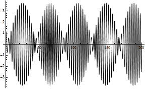
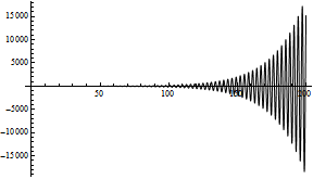
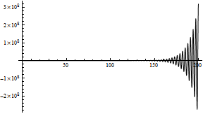
Figure 7. Solutions of (34) with $\xi(0)=\xi^{\prime}(0)=1$, $k=14$, $l=1$, $A\in\{0.79;0.8;0.81\}$.

When $A<0.75$ the behavior of $\xi$ appears periodic with, basically, oscillations of constant amplitude. When $A=0.79$ (left picture) the function $\xi$ still appears periodic but with oscillations of variable amplitude; this behavior always turned out to be the foreplay of instability. And, indeed, when $A=0.8$ we see (middle picture) that $\xi(t)$ oscillates with increasing amplitude and reaches a magnitude of the order of $10^{4}$ for $t=200$. The same phenomenon is accentuated for $A=0.81$ (right picture) where $\xi(200)$ has an order of magnitude of $10^{8}$. By increasing further $A$ the magnitude was also increasing. This is how we found $A_{1}(14)=0.8$.

From the values of $A_{1}(k)$ and $A_{2}(k)$ one can compute the corresponding energies $E_{1}$ and $E_{2}$ as given by (33):

(41) $$E_{l}(k)=(\gamma\mu_{k,1}+a_{k})\frac{A_{l}(k)^{2}}{2}+b_{k}\frac{A_{l}(k)^{4}}{4}\qquad(l=1,2)\,.$$

Then we can compute the flutter energy of the $k$-th longitudinal mode $\overline{\varphi}_{k}$ (see Definition 4.6) as

$$E_{k}=\min\{E_{1}(k),E_{2}(k)\}\,.$$

In Table 5 we quote our numerical results for some values of $\gamma$. In the middle table we use (40), that is, the value of $\gamma$ obtained from the parameters of the TNB. We found completely similar behaviors also for $\gamma=10^{-2}$ and $\gamma=5\cdot 10^{-5}$.

$k$	1	2	3	4	5	6	7	8	9	10	11	12	13	14
$A_{1}(k)$	4.62	2.96	2.93	2.85	2.67	2.31	1.42	$>$20	$>$20	$>$20	0.89	1.51	2.02	2.51
$A_{2}(k)$	5.93	9.23	5.91	5.87	5.79	5.63	5.36	4.92	4.19	2.62	$>$20	$>$20	$>$20	$>$20

$k$	1	2	3	4	5	6	7	8	9	10	11	12	13	14
$A_{1}(k)$	3.32	2.12	2.10	2.04	1.92	1.65	1.01	$>20$	$>20$	$>20$	0.62	1.08	1.46	1.82
$A_{2}(k)$	4.26	2.46	4.25	4.22	4.15	4.05	3.86	3.54	3.01	1.87	$>20$	$>20$	$>20$	$>20$

$k$	1	2	3	4	5	6	7	8	9	10	11	12	13	14
$A_{1}(k)$	1.44	0.91	0.9	0.88	0.82	0.69	$>$10	$>$10	$>$10	$>$10	0.2	0.44	0.63	0.8
$A_{2}(k)$	1.87	2.91	1.86	1.85	1.82	1.77	1.69	1.54	1.3	0.76	$>$10	$>$10	$>$10	$>$10

Table 5. Numerical values of $A_{1}(k)$ and $A_{2}(k)$ when $\gamma=10^{-3}$ (top), $\gamma=5.17\cdot 10^{-4}$ (middle), $\gamma=10^{-4}$ (bottom).

Remark 5.1.

From Table 5 we deduce that, if $\gamma=10^{-3}$ or $\gamma=5.17\cdot 10^{-4}$ then $A_{1}(k)>A_{2}(k)$ provided that $k=8,9,10$. If $\gamma=10^{-4}$ this happens provided that $k=7,8,9,10$. In these cases, the energy transfer occurs on the second torsional mode. On the contrary, for lower $k$, we have that $A_{1}(k)<A_{2}(k)$.

These results deserve several comments. First of all, we notice that the values of $A_{1}(1)$ and $A_{2}(2)$ are somehow out of the pattern because they are strongly influenced by the definition of the coefficients $d_{l,k}$ in (36) which is fairly different if $l=k$ and $l\neq k$. If we drop the case $k=l$, from Table 5 we see that the maps $k\mapsto A_{l}(k)$ are strictly decreasing until some $k$ where $A_{l}(k)$ becomes very large. In particular, when $l=2$ the least amplitude of oscillation $A_{2}(k)$ (threshold of instability) is obtained for $k=10$. This behavior is obtained for different values of $\gamma$. As pointed out in the Introduction, on the day of the TNB collapse the motions were considerably less than had occurred many times before. Table 5 gives an answer to question (Q3): the tenth longitudinal mode seems more prone to generate the second torsional mode.

6. Validation of the results

6.1. Validation of the linearization procedure

Fix some $k\in\{1,...,14\}$ and some $l\in\{1,2\}$. The energies $E_{l}(k)$ in (41) are computed in Section 5 with the following algorithm. Firstly we solve (32) and find the $k$-th longitudinal mode $\overline{\varphi}_{k}$ at energy $E(\phi_{0}^{k},\phi_{1}^{k})$. Then we use $\overline{\varphi}_{k}$ to determine the function $A_{l,k}(t)$ in (35). Finally, we study the stability of the trivial solution of (34): if it is stable then $E(\phi_{0}^{k},\phi_{1}^{k})<E_{l}(k)$ while if it is unstable, then $E(\phi_{0}^{k},\phi_{1}^{k})>E_{l}(k)$. With different choices of the initial data $(\phi_{0}^{k},\phi_{1}^{k})$ we are so able to find both upper and lower bounds which can be as close as wanted.

Overall, this algorithm means that we are solving the following system

(42) $$\begin{cases}\varphi^{\prime\prime}_{k}(t)+(\gamma\mu_{k,1}+a_{k})\varphi_{k}(t)+b_{k}\varphi_{k}^{3}(t)=0\qquad\forall t>0\\ \xi_{l}^{\prime\prime}(t)+(\gamma\nu_{l,2}+\bar{a}_{l}+d_{l,k}\varphi_{k}^{2}(t))\xi_{l}(t)=0\qquad\forall t>0\\ \varphi_{k}(0)=\phi_{0}^{k}\,,\quad\varphi_{k}^{\prime}(0)=\phi_{1}^{k}\\ \xi_{l}(0)=\varepsilon_{0}\,,\quad\xi_{l}^{\prime}(0)=\varepsilon_{1}\end{cases}$$

where $|\varepsilon_{1}|+|\varepsilon_{2}|\ll|\phi_{0}^{k}|+|\phi_{1}^{k}|$. The system (42) is obtained by putting to 0 all the $\varphi_{j}$ with $j\neq k$ and $\tau_{j}$ with $j\neq l$ in (28) and by linearizing the so found $2\times 2$ system of ODE’s in a neighborhood of the solution $(\overline{\varphi}_{k},0)$.

One may wonder if this method to determine $E_{l}(k)$ does not suffer from this linearization and give incorrect results. We have so tried a nonlinear approach and considered systems such as

(43) $$\begin{cases}\varphi^{\prime\prime}_{k}(t)+(\gamma\mu_{k,1}+a_{k})\varphi_{k}(t)+b_{k}\varphi_{k}^{3}(t)+\alpha_{1}\xi_{l}^{2}(t)\varphi_{k}(t)+\alpha_{2}\xi_{l}(t)\varphi_{k}^{2}(t)=0\qquad\forall t>0\\ \xi_{l}^{\prime\prime}(t)+(\gamma\nu_{l,2}+\bar{a}_{l}+d_{l,k}\varphi_{k}^{2}(t))\xi_{l}(t)+\beta_{1}\varphi_{k}(t)\xi_{l}^{2}(t)+\beta_{2}\xi_{l}^{3}(t)=0\qquad\forall t>0\\ \varphi_{k}(0)=\phi_{0}^{k}\,,\quad\varphi_{k}^{\prime}(0)=\phi_{1}^{k}\\ \xi_{l}(0)=\varepsilon_{0}\,,\quad\xi_{l}^{\prime}(0)=\varepsilon_{1}\,;\end{cases}$$

note that the equations in (43) differ from the ones in (42) by third order homogeneous polynomials with respect to $\varphi_{k}$ and $\xi_{l}$. We numerically solved (43) for different choices of the constants $\alpha_{i}$ and $\beta_{i}$ but, regardless of the choice, we always found that

the solution $\xi_{l}$ of (42) remains small for all $t>0$ if and only if the solution $\xi_{l}$ of (43) remains small for all $t>0$.

This behavior had to be expected in view of the theoretical result in [26].

This means that the computation of $E_{l}(k)$ (and of the flutter energy of the $k$-th longitudinal mode) does not depend on the linearization procedure. Moreover, this shows that Definition 4.3 well characterizes the stability of the $k$-th longitudinal mode with respect to the $l$-th torsional mode.

6.2. Different nonlinearities: a system of Hill equations

For any longitudinal mode $k$, the just described procedure with the specific nonlinearity chosen, see (20), yields the system (34) of uncoupled Hill equations ($l=1,2$). This enables us to study separately the stability of each of the two equations in (34) and to compute the thresholds $A_{l}(k)$ as described above.

For different nonlinearities, other than (20), it may happen that the corresponding equations in (34) ($l=1,2$) remain coupled and give rise to a Hill system of the form

(44) $$\Xi^{\prime\prime}(t)+A_{l,k}(t)\Xi(t)=0$$

where $\Xi=(\xi_{1},\xi_{2})$ and $A_{l,k}$ is now a $2\times 2$ periodic matrix. In this case, one should investigate the stability of the trivial solution $\Xi\equiv(0,0)$ of (44). By [35, Theorem II p.270, vol.1] we know that this trivial solution is stable provided that the trivial solutions of a family of related Hill equations are stable. Therefore, even for different nonlinearities or for a larger number of torsional modes, the stability of the $k$-th longitudinal mode with respect to the torsional components may be performed through a finite number of stability analysis of some Hill equations.

6.3. The coupled nonlinear system

In this section we discuss the nonlinear system (28) with $\gamma=5.17\cdot 10^{-4}$ as for the TNB, see (40). We provide an alternative notion of stability for a solution of (28) having the torsional components $\tau_{1}$ and $\tau_{2}$ identically equal to zero. Then we discuss the stability of the longitudinal components. Our purpose is to explain to which extent the decoupling procedure applied in Section 4.2 provides an accurate description of the phenomena.

For our convenience we slightly modify some notations. We denote by $\widetilde{w}_{1},\dots,\widetilde{w}_{14}$ the first fourteen eigenfunctions (see Section 4.2) which are even with respect to $y$, i.e. $\widetilde{w}_{k}=w_{k}$ for any index $k\in\{1,\dots,10\}$ and $\widetilde{w}_{11}=w_{12}$, $\widetilde{w}_{12}=w_{13}$, $\widetilde{w}_{13}=w_{14}$, $\widetilde{w}_{14}=w_{15}$. Then we denote by $\widetilde{w}_{15}=w_{10}$ and $\widetilde{w}_{16}=w_{16}$ as the first two eigenfunctions which are odd with respect to $y$. All the eigenfunctions are normalized in $L^{2}(\Omega)$. Similarly we relabel the functions $\varphi_{1},\dots,\varphi_{14}$ and $\tau_{1},\tau_{2}$ as $\widetilde{\varphi}_{k}$ for $k\in\{1,...,16\}$ and the corresponding eigenvalues $\widetilde{\mu}_{k}$ for any $k\in\{1,\dots,16\}$. Then, for $\Upsilon$ as in (20), we introduce the constants

$$A_{k}=\int_{\Omega}\Upsilon(y)\widetilde{w}_{k}^{2}\,dxdy\quad\text{for any }k\in\{1,\dots,16\}$$

and for any $j_{1},j_{2},j_{3}\in\{1,\dots,16\}$, $j_{1}\geqslant j_{2}\geqslant j_{3}$ and $k\in\{1,\dots,16\}$

(45) $$B_{j_{1}j_{2}j_{3}k}=\begin{cases}\int_{\Omega}\Upsilon(y)\widetilde{w}_{j_{1}}\widetilde{w}_{j_{2}}\widetilde{w}_{j_{3}}\widetilde{w}_{k}\,dxdy&\quad\text{if }j_{1}=j_{2}=j_{3}\\[8.0pt] 3\int_{\Omega}\Upsilon(y)\widetilde{w}_{j_{1}}\widetilde{w}_{j_{2}}\widetilde{w}_{j_{3}}\widetilde{w}_{k}\,dxdy&\quad\text{if }j_{1}>j_{2}=j_{3}\ \text{or}\ j_{1}=j_{2}>j_{3}\\[8.0pt] 6\int_{\Omega}\Upsilon(y)\widetilde{w}_{j_{1}}\widetilde{w}_{j_{2}}\widetilde{w}_{j_{3}}\widetilde{w}_{k}\,dxdy&\quad\text{if }j_{1}>j_{2}>j_{3}\,.\end{cases}$$

With these notations we may write (28) and the corresponding initial conditions in the form

(46) $$\begin{cases}\displaystyle{\widetilde{\varphi}_{k}^{\prime\prime}(t)+(\gamma\widetilde{\mu}_{k}+A_{k})\widetilde{\varphi}_{k}(t)+\sum_{\underset{j_{1}\geqslant j_{2}\geqslant j_{3}}{j_{1},j_{2},j_{3}=1}}^{16}B_{j_{1}j_{2}j_{3}k}\,\widetilde{\varphi}_{j_{1}}(t)\widetilde{\varphi}_{j_{2}}(t)\widetilde{\varphi}_{j_{3}}(t)=0\,,}&\qquad k\in\{1,\dots,16\}\,,\\[25.0pt] \widetilde{\varphi}_{k}(0)=\widetilde{\phi}_{0}^{k}\,,\quad\widetilde{\varphi}_{k}^{\prime}(0)=\widetilde{\phi}_{1}^{k}\,,&\qquad k\in\{1,\dots,16\}\,.\end{cases}$$

We observe that if $k=15,16$ then $B_{j_{1}j_{2}j_{3}k}=0$ for any $j_{1},j_{2},j_{3}\in\{1,\dots,14\}$ such that $j_{1}\geqslant j_{2}\geqslant j_{3}$; therefore if we choose $\widetilde{\phi}_{0}^{15}=\widetilde{\phi}_{1}^{15}=\widetilde{\phi}_{0}^{16}=\widetilde{\phi}_{1}^{16}=0$, then the solution of (46) satisfies $\widetilde{\varphi}_{15}=\widetilde{\varphi}_{16}\equiv 0$. This means that no torsional oscillation may appear if such a kind of oscillation equals zero at $t=0$. We summarize this fact in the following

Proposition 6.1.

The unique solution $(\widetilde{\varphi}_{1},...,\widetilde{\varphi}_{16})$ of (46) with $\widetilde{\phi}_{0}^{15}=\widetilde{\phi}_{1}^{15}=\widetilde{\phi}_{0}^{16}=\widetilde{\phi}_{1}^{16}=0$ satisfies $\widetilde{\varphi}_{15}(t)=\widetilde{\varphi}_{16}(t)=0$ for any $t\in{\mathbb{R}}$.

The situation is completely different if we do not assume that $\widetilde{\phi}_{0}^{15}=\widetilde{\phi}_{1}^{15}=\widetilde{\phi}_{0}^{16}=\widetilde{\phi}_{1}^{16}=0$: in this case the first fourteen equations are coupled with the last two since the $B_{kj_{2}j_{3}k}$ may be different from zero if $k\in\{15,16\}$ and $j_{2},j_{3}\leqslant 14$. This suggests to make precise how an oscillation mode may influence the others.

Definition 6.2.

Let us consider system (46).

• We say that the $k$-th mode influences the $j$-th mode ($j\neq k$) if $B_{kkkj}\neq 0$.

• We say that the $k_{1}$-th and $k_{2}$-th modes ($k_{1}>k_{2}$) influence the $j$-th mode ($j\not\in\{k_{1},k_{2}\}$) if at least one between $B_{k_{1}k_{1}k_{2}j}$ or $B_{k_{1}k_{2}k_{2}j}$ is different from zero.

• We say that the $k_{1}$-th, $k_{2}$-th, $k_{3}$-th modes ($k_{1}>k_{2}>k_{3}$) influence the $j$-th mode ($j\not\in\{k_{1},k_{2},k_{3}\}$) if $B_{k_{1}k_{2}k_{3}j}\neq 0$.

If some modes influence the $j$-th mode it may happen that, in system (46), $\widetilde{\varphi}_{j}\not\equiv 0$ even if $(\widetilde{\phi}_{0}^{j},\widetilde{\phi}_{1}^{j})=(0,0)$. We state a result which explains how longitudinal modes influence each other.

Proposition 6.3.

The following statements hold true:

• Let $k,j\in\{1,\dots,14\}$ with $j\neq k$. If $j=3k$ then the $k$-th mode influences the $j$-th mode;

• Let $k_{1},k_{2},j\in\{1,\dots,14\}$ with $k_{1}>k_{2}$ and $j\not\in\{k_{1},k_{2}\}$. If $j\in\{2k_{1}+k_{2},2k_{1}-k_{2},k_{1}+2k_{2},|k_{1}-2k_{2}|\}$ then the $k_{1}$-th and $k_{2}$-th modes influence the $j$-th mode.

• Let $k_{1},k_{2},k_{3},j\in\{1,\dots,14\}$ with $k_{1}>k_{2}>k_{3}$ and $j\not\in\{k_{1},k_{2},k_{3}\}$. If $j\in\{k_{1}+k_{2}+k_{3},k_{1}+k_{2}-k_{3},k_{1}-k_{2}+k_{3},|k_{1}-k_{2}-k_{3}|\}$ then the $k_{1}$-th, $k_{2}$-th and $k_{3}$-th modes influence the $j$-th mode.

Proof.

In order to treat (i)-(ii) together we assume that $k_{1}\geqslant k_{2}$ where also equality is admissible. Then, under the assumptions of the proposition we infer that either $B_{k_{1}k_{1}k_{2}j}\neq 0$ or $B_{k_{1}k_{2}k_{2}j}\neq 0$ since either $\int_{0}^{\pi}\sin(k_{1}x)\sin(k_{1}x)\sin(k_{2}x)\sin(jx)\,dx\neq 0$ or $\int_{0}^{\pi}\sin(k_{1}x)\sin(k_{2}x)\sin(k_{2}x)\sin(jx)\,dx\neq 0$ thanks to Werner formulas; moreover $v_{k}(y)>0$ for any $y\in\left(-\frac{\pi}{150},\frac{\pi}{150}\right)$ and $k\in\{1,\dots,14\}$, with $v_{k}$ as in Section 4.2. The case (iii) can be treated in a similar way. ∎

Remark 6.4.

Proposition 6.3 strongly depends on the nonlinearity $h$ introduced in (20). That the $k$-th mode influences the $j$-th mode when $j=3k$ (statement (i)) depends on the fact that the nonlinearity $h(y,u)$ contains a cubic term. If the cubic term is replaced with a different term then the influences may vary. A similar discussion is valid for (ii)-(iii) in Proposition 6.3.

To illustrate Proposition 6.3, we consider the case where $\widetilde{\phi}_{0}^{1}=1$, $\widetilde{\phi}_{1}^{1}=0$ and $\widetilde{\phi}_{0}^{k}=\widetilde{\phi}_{1}^{k}=0$ for all $k\in\{2,\dots,16\}$. According to Proposition 6.3, the first longitudinal mode influences only the third longitudinal mode but this does not mean that only $\widetilde{\varphi}_{1}$ and $\widetilde{\varphi}_{3}$ are nontrivial in (46). As one can see from Figure 8 below, where a numerical solution of (46) is obtained, also the functions $\widetilde{\varphi}_{5},\widetilde{\varphi}_{7},\widetilde{\varphi}_{9},\widetilde{\varphi}_{11},\widetilde{\varphi}_{13}$ are not identically equal to zero while all the other longitudinal modes and the two torsional modes are identically equal to zero.

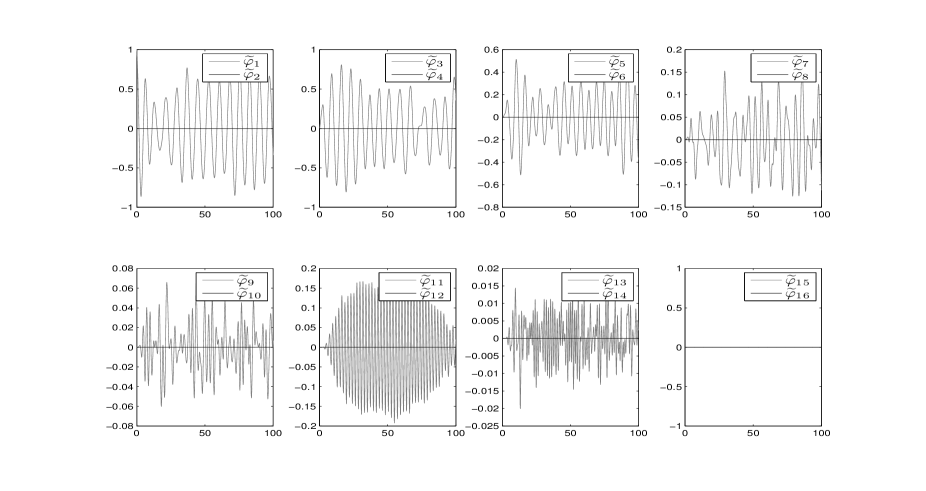
Figure 8. The solution of (46) with $\widetilde{\phi}_{0}^{1}=1$, $\widetilde{\phi}_{1}^{1}=0$, $(\widetilde{\phi}_{0}^{k},\widetilde{\phi}_{1}^{k})=(0,0)$ for any $k\in\{2,\dots,16\}$.

Let us briefly discuss these results. From Proposition 6.3 (i) with $k=1$ and $j=3$, we deduce that $\widetilde{\varphi}_{1}$ influences $\widetilde{\varphi}_{3}$; by Proposition 6.3 (ii) with $k_{1}=3$ and $k_{2}=1$ we have that $\widetilde{\varphi}_{1}$ and $\widetilde{\varphi}_{3}$ influence $\widetilde{\varphi}_{5}$. Then $\widetilde{\varphi}_{1}$ and $\widetilde{\varphi}_{5}$ influence $\widetilde{\varphi}_{7}$. In the next stages $\widetilde{\varphi}_{1}$ and $\widetilde{\varphi}_{7}$ influence $\widetilde{\varphi}_{9}$, while $\widetilde{\varphi}_{1}$ and $\widetilde{\varphi}_{9}$ influence $\widetilde{\varphi}_{11}$; finally $\widetilde{\varphi}_{1}$ and $\widetilde{\varphi}_{11}$ influence $\widetilde{\varphi}_{13}$.

As a second example we consider $\widetilde{\phi}_{0}^{2}=1$, $\widetilde{\phi}_{1}^{2}=0$ and $(\widetilde{\phi}_{0}^{k},\widetilde{\phi}_{1}^{k})=(0,0)$ for any $k\in\{1,\dots,16\}$ with $k\neq 2$. A similar phenomenon occurs as one can see from Figure 9 below.

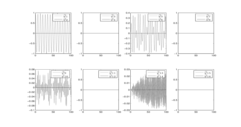
Figure 9. The solution of (46) with $\widetilde{\phi}_{0}^{2}=1$, $\widetilde{\phi}_{1}^{2}=0$, $(\widetilde{\phi}_{0}^{k},\widetilde{\phi}_{1}^{k})=(0,0)$ for any $k\in\{1,\dots,16\}$, $k\neq 2$.

One can observe that only the functions $\widetilde{\varphi}_{2}$, $\widetilde{\varphi}_{6}$, $\widetilde{\varphi}_{10}$, $\widetilde{\varphi}_{14}$ are not identically equal to zero.

A further consequence of our approach deserves to be emphasized. We have truncated an infinite dimensional system up the least 16 modes: although this truncation is legitimate for energy reasons (see [8]), it may lead to some small glitches. Since we are considering a truncated system with fourteen longitudinal modes and two torsional modes, it happens that if $k\in\{5,\dots,14\}$ then the mode $\widetilde{\varphi}_{k}$ influences no other modes, hence the solution of (46) with $(\widetilde{\phi}_{0}^{k},\widetilde{\phi}_{1}^{k})\neq(0,0)$ and $(\widetilde{\phi}_{0}^{j},\widetilde{\phi}_{1}^{j})=(0,0)$ for any $j\in\{1,\dots,16\}$, $j\neq k$, satisfies $\widetilde{\varphi}_{k}\not\equiv 0$ and $\widetilde{\varphi}_{j}\equiv 0$ for any $j\in\{1,\dots,16\}$, $j\neq k$. This is another consequence of Proposition 6.3 (i) which can be summarized in the following

Proposition 6.5.

Let $k\in\{5,\dots,14\}$. Suppose that $(\widetilde{\phi}_{0}^{k},\widetilde{\phi}_{1}^{k})\neq(0,0)$ and that $(\widetilde{\phi}_{0}^{j},\widetilde{\phi}_{1}^{j})=(0,0)$ for any $j\in\{1,\dots,16\}$, $j\neq k$. Then the corresponding solution of (46) satisfies

$$\widetilde{\varphi}_{j}(t)=0\qquad\text{for any }t\in{\mathbb{R}}\quad\text{and}\quad j\in\{1,\dots,16\},j\neq k\,.$$

6.4. Comparison of the results for the coupled and uncoupled systems

In this section we show that the responses of the truncated system (46) are in line with the theoretical and numerical responses obtained from the Hill equation (34) in Sections 4.3 and 5.

We first provide the definition of stability of solutions of (46) satisfying $(\widetilde{\phi}_{0}^{15},\widetilde{\phi}_{1}^{15})=(\widetilde{\phi}_{0}^{16},\widetilde{\phi}_{1}^{16})=(0,0)$, namely solutions of

($$P_{0} \begin{cases}\displaystyle{\widetilde{\varphi}_{k}^{\prime\prime}(t)+(\gamma\widetilde{\mu}_{k}+A_{k})\widetilde{\varphi}_{k}(t)+\sum_{\underset{j_{1}\geqslant j_{2}\geqslant j_{3}}{j_{1},j_{2},j_{3}=1}}^{16}B_{j_{1}j_{2}j_{3}k}\,\widetilde{\varphi}_{j_{1}}(t)\widetilde{\varphi}_{j_{2}}(t)\widetilde{\varphi}_{j_{3}}(t)=0\,,}&\ \ k\in\{1,\dots,16\}\,,\\[25.0pt] \widetilde{\varphi}_{k}(0)=\widetilde{\phi}_{0}^{k}\,,\quad\widetilde{\varphi}_{k}^{\prime}(0)=\widetilde{\phi}_{1}^{k}\,,&\ \ k\in\{1,\dots,14\}\,,\\[10.0pt] \widetilde{\varphi}_{15}(0)=\widetilde{\varphi}^{\prime}_{15}(0)=\widetilde{\varphi}_{16}(0)=\widetilde{\varphi}^{\prime}_{16}(0)=0\,.\end{cases}$$)

In the sequel a solution of ($P_{0}$) will be denoted by $\Phi_{0}=(\widetilde{\varphi}_{1},\dots,\widetilde{\varphi}_{14},0,0)$, see Proposition 6.1. We also denote by $\Phi=(\widetilde{\varphi}_{1},\dots,\widetilde{\varphi}_{16})$ a general solution of (46).

Definition 6.6.

Let $\widetilde{\phi}_{0}^{1},\dots,\widetilde{\phi}_{0}^{14}$ and $\widetilde{\phi}_{1}^{1},\dots,\widetilde{\phi}_{1}^{14}$ be fixed and let $\Phi_{0}$ be the corresponding solution of ($P_{0}$).

• We say that a solution $\Phi_{0}$ of ($P_{0}$) is stable with respect to the first torsional mode if for any $\varepsilon>0$ there exists $\delta>0$ such that if $\max\{|\widetilde{\phi}_{0}^{15}|,|\widetilde{\phi}_{1}^{15}|\}<\delta$ and $(\widetilde{\phi}_{0}^{16},\widetilde{\phi}_{1}^{16})=(0,0)$, then the solution $\Phi$ of (46) corresponding to $\widetilde{\phi}_{0}^{1},\dots,\widetilde{\phi}_{0}^{16}$ and $\widetilde{\phi}_{1}^{1},\dots,\widetilde{\phi}_{1}^{16}$ satisfies

  $$|\widetilde{\varphi}_{15}(t)|<\varepsilon\,,\quad|\widetilde{\varphi}_{15}^{\prime}(t)|<\varepsilon\qquad\text{for any }t\in{\mathbb{R}}\,.$$

• We say that a solution $\Phi_{0}$ of ($P_{0}$) is stable with respect to the second torsional mode if for any $\varepsilon>0$ there exists $\delta>0$ such that if $\max\{|\widetilde{\phi}_{0}^{16}|,|\widetilde{\phi}_{1}^{16}|\}<\delta$ and $(\widetilde{\phi}_{0}^{15},\widetilde{\phi}_{1}^{15})=(0,0)$, then the solution $\Phi$ of (46) corresponding to $\widetilde{\phi}_{0}^{1},\dots,\widetilde{\phi}_{0}^{16}$ and $\widetilde{\phi}_{1}^{1},\dots,\widetilde{\phi}_{1}^{16}$ satisfies

  $$|\widetilde{\varphi}_{16}(t)|<\varepsilon\,,\quad|\widetilde{\varphi}_{16}^{\prime}(t)|<\varepsilon\qquad\text{for any }t\in{\mathbb{R}}\,.$$

Definition 6.6 should be compared with Definition 4.3. So far, to find sufficient conditions on $\Phi_{0}$ which guarantee its stability with respect to one of the torsional modes (according to Definition 6.6) seems out of reach. However, Theorems 4.4 and 4.5 suggest the following

Conjecture 6.7.

Let $l\in\{1,2\}$. There exists $A_{l}>0$ such that if

$$\max\{|\widetilde{\phi}_{0}^{1}|,\dots,|\widetilde{\phi}_{0}^{14}|,|\widetilde{\phi}_{1}^{1}|,\dots,|\widetilde{\phi}_{1}^{14}|\}<A_{l}$$

then the corresponding solution $\Phi_{0}$ of ($P_{0}$) is stable with respect to the $l$-th torsional mode.

Our purpose is to support Conjecture 6.7 from a numerical point of view under suitable restrictions on the values of the initial conditions $\widetilde{\phi}_{0}^{1},\dots,\widetilde{\phi}_{0}^{14},\widetilde{\phi}_{1}^{1},\dots,\widetilde{\phi}_{1}^{14}$ in ($P_{0}$). For more numerical results concerning Conjecture 6.7 we refer to [7].

For any $k\in\{1,\dots,14\}$ we consider the problem

($$P_{0,k} \begin{cases}\displaystyle{\widetilde{\varphi}_{j}^{\prime\prime}(t)+(\gamma\widetilde{\mu}_{j}+A_{j})\widetilde{\varphi}_{j}(t)+\sum_{\underset{j_{1}\geqslant j_{2}\geqslant j_{3}}{j_{1},j_{2},j_{3}=1}}^{16}B_{j_{1}j_{2}j_{3}j}\,\widetilde{\varphi}_{j_{1}}(t)\widetilde{\varphi}_{j_{2}}(t)\widetilde{\varphi}_{j_{3}}(t)=0\,,}&\ \ j\in\{1,\dots,16\}\,,\\[25.0pt] \widetilde{\varphi}_{k}(0)=A\,,\quad\widetilde{\varphi}_{k}^{\prime}(0)=0\,,\\[10.0pt] \widetilde{\varphi}_{j}(0)=\widetilde{\varphi}^{\prime}_{j}(0)=0\,,&\ \ j\in\{1,\dots,16\}\,,j\neq k\,.\end{cases}$$)

Then for any $k\in\{1,\dots,14\}$ and $l\in\{15,16\}$ we also consider the following perturbation of ($P_{0,k}$)

($$P_{\delta,k,l} \begin{cases}\displaystyle{\widetilde{\varphi}_{j}^{\prime\prime}(t)+(\gamma\widetilde{\mu}_{j}+A_{j})\widetilde{\varphi}_{j}(t)+\sum_{\underset{j_{1}\geqslant j_{2}\geqslant j_{3}}{j_{1},j_{2},j_{3}=1}}^{16}B_{j_{1}j_{2}j_{3}j}\,\widetilde{\varphi}_{j_{1}}(t)\widetilde{\varphi}_{j_{2}}(t)\widetilde{\varphi}_{j_{3}}(t)=0\,,}\qquad\quad j\in\{1,\dots,16\}\,,\\[25.0pt] \widetilde{\varphi}_{k}(0)=A\,,\quad\widetilde{\varphi}_{k}^{\prime}(0)=0\,,\\[10.0pt] \widetilde{\varphi}_{l}(0)=\widetilde{\varphi}_{l}^{\prime}(0)=\delta\,,\\[10.0pt] \widetilde{\varphi}_{j}(0)=\widetilde{\varphi}^{\prime}_{j}(0)=0\,,\qquad\qquad\qquad\qquad\qquad\qquad j\in\{1,\dots,16\}\,,j\neq k\,,j\neq l\,.\end{cases}$$)

In the particular case of solutions of ($P_{0,k}$), Conjecture 6.7 reads

for any $l\in\{1,2\}$ and $k\in\{1,\dots,14\}$ there exists $\widetilde{A}_{l}(k)>0$ such that for any $A\in(0,\widetilde{A}_{l}(k))$ the solution $\Phi_{0}$ of ($P_{0,k}$) is stable with respect to the $l$-th torsional mode  .

Numerical simulations give the approximate values of $\widetilde{A}_{l}(k)$ as reported in Table 6.

$k$	1	2	3	4	5	6	7	8	9	10	11	12	13	14
$\widetilde{A}_{1}(k)$	2.38	1.89	3.83	2.27	1.92	1.66	1.02	$>10$	$>10$	$>10$	0.62	1.08	1.46	1.83
$\widetilde{A}_{2}(k)$	5.17	4.38	4.94	8.08	4.18	4.05	3.87	3.59	3.10	1.87	$>10$	$>10$	$>10$	$>10$

Table 6. Numerical values of $\widetilde{A}_{1}(k)$ and $\widetilde{A}_{2}(k)$ when $\gamma=5.17\cdot 10^{-4}$.

Remark 6.8.

From Table 6 we see that $\widetilde{A}_{1}(k)>\widetilde{A}_{2}(k)$ provided that $k=8,9,10$ whereas for lower $k$ we have that $\widetilde{A}_{1}(k)<\widetilde{A}_{2}(k)$.

Let us explain how we obtained Table 6. As a particular example we take the value of $A_{1}(5)$. In Figure 10 we plot the graph of the component $\widetilde{\varphi}_{5}$ of the solution $\Phi_{0}$ of ($P_{0,k}$) with $k=5$ and $A=1.92$.

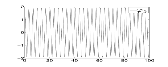
Figure 10. The component $\widetilde{\varphi}_{5}$ of the solution $\Phi_{0}$ of ($P_{0,k}$) with $k=5$ and $A=1.92$.

The instability phenomenon appearing for $A=1.92$ is represented in Figure 11 where we see that the amplitude of the oscillations of $\widetilde{\varphi}_{15}$ is fairly wide for large $t$ even if we choose a small value of $\delta$ in ($P_{\delta,k,l}$).

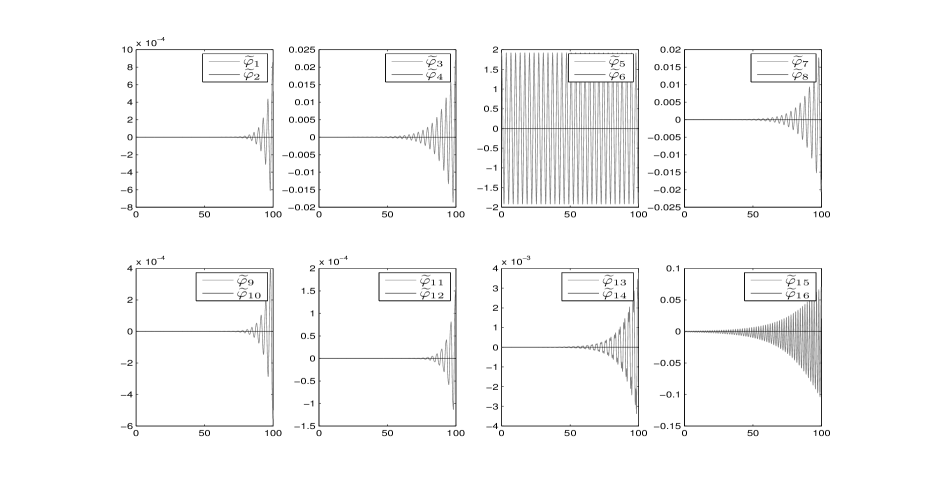
Figure 11. The components of the solution $\Phi$ of ($P_{\delta,k,l}$) with $k=5$, $l=15$, $A=1.92$ and $\delta=5\cdot 10^{-4}$.

On the other hand, if we choose $A=1.91$ we see in Figure 12 that the amplitude of the oscillations of $\widetilde{\varphi}_{15}$ remains of the same order of magnitude also when $t$ is large. This is how we obtained $A_{1}(5)=1.92$ in Table 6.

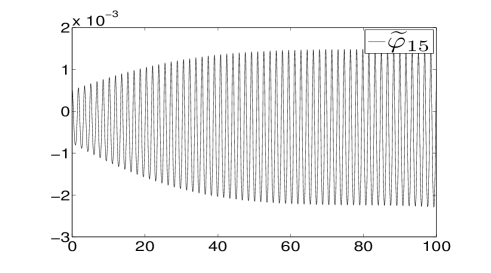
Figure 12. The function $\widetilde{\varphi}_{15}$ corresponding to the solution of ($P_{\delta,k,l}$) with $k=5$, $l=15$, $A=1.91$ and $\delta=5\cdot 10^{-4}$.

The comparison between Table 6 and Table 5 (middle table for $\gamma=5.17\cdot 10^{-4}$) deserves several comments. The values of $\widetilde{A}_{1}(k)$ when $k\in\{5,\dots,14\}\setminus\{8,9,10\}$ and of $\widetilde{A}_{2}(k)$ when $k\in\{5,\dots,10\}$ are very close to the corresponding ones of $A_{1}(k)$ and $A_{2}(k)$ in Table 5. The reason is that for these values of $k$ the solution $\Phi_{0}$ of ($P_{0,k}$) satisfies $\widetilde{\varphi}_{j}\equiv 0$ for any $j\neq k$, see Proposition 6.5, hence the equations are decoupled.

Then, with the same choice of $k$, fix $\delta>0$, $l\in\{15,16\}$ and let $\Phi_{\delta}$ be the corresponding solution of ($P_{\delta,k,l}$). If $\delta$ is small enough the function $\Phi_{\delta}$ is expected to be close to $\Phi_{0}$ until $\widetilde{\varphi}_{l}$ remains small together with its derivative. And indeed, if we chose $k=5$, $l=15$, $A=1.92$, $\delta=5\cdot 10^{-4}$, we numerically obtain the plots of Figure 11.

We also observe that for larger values of $A$, say $A=1.94$, when the fifteenth component of $\Phi_{\delta}$ is no longer “negligible” the values of the fifth component $\widetilde{\varphi}_{5}$ of $\Phi_{\delta}$ are considerably different from the values of the fifth component of $\Phi_{0}$, at least for large $t$: in the latter case $\widetilde{\varphi}_{5}$ is periodic while in the former case $\widetilde{\varphi}_{5}$ exhibits a variation in the amplitude of the oscillations soon after the amplitude of the oscillations of the fifteenth component has become relatively large, as one can see from Figure 13.

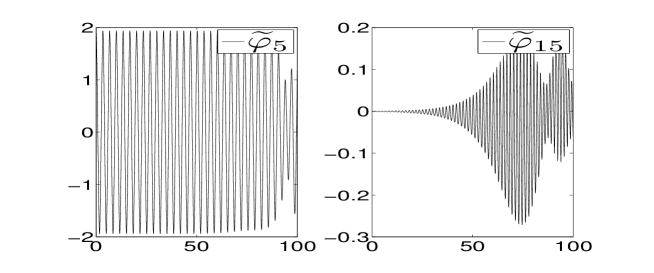
Figure 13. The functions $\widetilde{\varphi}_{5}$ and $\widetilde{\varphi}_{15}$ corresponding to the solution $\Phi$ of ($P_{0,k}$) with $k=5$ and $A=1.94$.

The critical values $\widetilde{A}_{1}(8)$, $\widetilde{A}_{1}(9)$, $\widetilde{A}_{1}(10)$, $\widetilde{A}_{2}(11)$, $\widetilde{A}_{2}(12)$, $\widetilde{A}_{2}(13)$, $\widetilde{A}_{2}(14)$ are very large in both Tables 5 and 6. No evident instability behavior was detected when considering solutions of (32) and (34) on one hand and solutions of ($P_{\delta,k,l}$) on the other hand.

It remains to discuss the cases where $k\in\{1,2,3,4\}$ for which the values of $\widetilde{A}_{1}(k)$ and $\widetilde{A}_{2}(k)$ in Table 6 are quite different from the values of $A_{1}(k)$ and $A_{2}(k)$ in the middle Table 5. By looking at Figures 8 and 9 one can see the graphs of the components of $\Phi_{0}$, the solution of ($P_{0,k}$), respectively in the cases $k=1$ and $k=2$ (for the two remaining cases $k=3,4$ we refer to [7]). In the two figures one observes that the $k$-th component of $\Phi_{0}$ is not the only large one, there are several other large components. In this case, the reduction of (46) to equations (32) and (34) is not a good approximation of the real situation.

6.5. Thresholds of stability in the TNB

In this subsection, starting from the values obtained in Table 6, we provide estimates on the thresholds of stability for the TNB by using the isolated system (14) with the values of the parameters given in Section 5. According to the notations of Subsection 6.3, we denote by $\widetilde{w}_{k}$, $k\in\{0,\dots,14\}$ the first fourteen longitudinal eigenfunctions normalized in $L^{2}(\Omega)$. For any $k\in\{0,\dots,14\}$ and $l\in\{1,2\}$ we choose the initial conditions in (14) in the form

(47) $$u_{0}(x,y)=\widetilde{A}_{l}(k)\widetilde{w}_{k}(x,y)\,,\quad u_{1}(x,y)=0\qquad\text{for any }(x,y)\in(0,\pi)\times(-\ell,\ell)$$

where the $\widetilde{A}_{l}(k)$ are as in Table 6. Our purpose is to provide, for any $k\in\{1,\dots,14\}$, the values measured in meters of the stability threshold for the energy transfer from the $k$-th longitudinal mode to a torsional mode. This will give an idea of the initial displacement of the deck sufficient to activate the torsional oscillations. To this end, we first give in Table 7 the approximate values of the $L^{\infty}$-norms of the $L^{2}$-normalized eigenfunctions.

$k$	1	2	3	4	5	6	7	8	9	10	11	12	13	14
$\|\widetilde{w}_{k}\|_{L^{\infty}}$ ​	​3.897​	​3.899​	​3.899​	​3.900​	​3.901​	​3.902​	​3.904​	​3.905​	​3.907​	​3.909​	​3.912​	​3.914​	​3.917​	​3.920

Table 7. Approximate values of $\|\widetilde{w}_{k}\|_{L^{\infty}}$ for $k\in\{1,\dots,14\}$.

By (47), Table 6, Table 7 and (12) with $k_{1}=k_{2}=\frac{6000H}{L^{3}}$ we obtain the following table which shows that the instability amplitude has the same order of magnitude as observed for the TNB, see [33].

$k$	1	2	3	4	5	6	7	8	9	10	11	12	13	14
$\|u_{0}\|_{L^{\infty}}$	​9.27​	​7.37​	​14.93​	​8.85​	​7.45​	​6.48​	​3.98​	​$>40$​	​$>40$​	​$>40$​	​2.43​	​4.23​	​5.72​	​7.17
$\|u_{0}\|_{L^{\infty}}$	​20.15​	​17.08​	​19.26​	​31.51​	​16.30​	​15.80​	​15.11​	​14.02​	​12.11​	​7.31​	​$>40$​	​$>40$​	​$>40$​	​$>40$

Table 8. The $L^{\infty}$-norm of $u_{0}$ measured in meters corresponding to the stability threshold of the $k$-th longitudinal mode with respect to the first torsional mode (first line) and the second torsional mode (second line).

7. Proof of Theorem 4.4

Assume that $1\leqslant k\leqslant 14$ and $l\in\{1,2\}$ are given. We introduce two constants which will be useful in the sequel. We set

(48) $$\delta_{l}:=\gamma\nu_{l,2}+\bar{a}_{l}\,,\qquad\rho_{k}:=\gamma\mu_{k,1}+a_{k}\,.$$

Using the definition of $\rho_{k}$ in (48), for any $E>0$ we put

(49) $$\Lambda_{\pm}^{k}(E)=\frac{\sqrt{\rho_{k}^{2}+4b_{k}E}\pm\rho_{k}}{b_{k}}\,.$$

Then (33) reads

(50) $$(\overline{\varphi}^{\prime}_{k})^{2}=\frac{b_{k}}{2}(\Lambda_{+}^{k}(E)+\overline{\varphi}_{k}^{2})(\Lambda_{-}^{k}(E)-\overline{\varphi}_{k}^{2})\,.$$

Hence, since any $k$-th longitudinal mode $\overline{\varphi}_{k}$ satisfies (33), we deduce

(51) $$\|\overline{\varphi}_{k}\|_{\infty}=\sqrt{{\Lambda_{-}^{k}(E)}}\,.$$

Since in the equation (32) there are only odd terms, the period $T_{k}(E)$ of $\overline{\varphi}_{k}$ is the double of the width of an interval of monotonicity of $\overline{\varphi}_{k}$. As the problem is autonomous, we may assume that $\overline{\varphi}_{k}(0)=-\|\overline{\varphi}_{k}\|_{\infty}$ and $\overline{\varphi}_{k}^{\prime}(0)=0$. By symmetry and periodicity we then have that $\overline{\varphi}_{k}(T_{k}/2)=\|\overline{\varphi}_{k}\|_{\infty}$ and $\overline{\varphi}_{k}^{\prime}(T_{k}/2)=0$. In the first interval of monotonicity of $\overline{\varphi}_{k}$ we may take the square root of (50) and obtain

(52) $$\overline{\varphi}^{\prime}_{k}(t)=\sqrt{\frac{b_{k}}{2}(\Lambda_{+}^{k}(E)+\overline{\varphi}_{k}^{2}(t))(\Lambda_{-}^{k}(E)-\overline{\varphi}_{k}^{2}(t))}\qquad\forall t\in\left[0,\frac{T_{k}}{2}\right]\,.$$

By separating variables, and integrating over the interval $(0,T_{k}/2)$ we obtain

$$\frac{T_{k}(E)}{2}=\sqrt{\frac{2}{b_{k}}}\int_{-\|\overline{\varphi}_{k}\|_{\infty}}^{\|\overline{\varphi}_{k}\|_{\infty}}\frac{ds}{\sqrt{(\Lambda_{+}^{k}(E)+s^{2})(\Lambda_{-}^{k}(E)-s^{2})}}\,.$$

Using the fact that the integrand is even with respect to $s$ and with a change of variable we get

(53) $$T_{k}(E)=\frac{4\sqrt{2}}{\sqrt{b_{k}}}\int_{0}^{1}\frac{ds}{\sqrt{(\Lambda_{+}^{k}(E)+\Lambda_{-}^{k}(E)s^{2})(1-s^{2})}}\,.$$

In particular,

(54) $$\mbox{the map }E\mapsto T_{k}(E)\mbox{ is strictly decreasing and }\lim_{E\to 0}T_{k}(E)=T_{k}(0)=\frac{2\pi}{\sqrt{\rho_{k}}}\,.$$

Let us prove the following sufficient condition for the torsional stability of $\overline{\varphi}_{k}$.

Lemma 7.1.

If there exists an integer $m$ such that

(55) $$\frac{4m^{2}\pi^{2}}{\delta_{l}}\leqslant T_{k}(E)^{2}\leqslant\frac{4(m+1)^{2}\pi^{2}}{\delta_{l}+d_{l,k}\Lambda_{-}^{k}(E)}$$

then $\overline{\varphi}_{k}$ is stable with respect to the $l$-th torsional mode.

Proof.

With the initial conditions $\xi(0)=\dot{\xi}(0)=0$, the unique solution of (34) is $\xi\equiv 0$. The statement follows if we prove that (55) is a sufficient condition for the trivial solution $\xi\equiv 0$ to be stable in the Lyapunov sense, namely if the solutions of (34) with small initial data $|\xi(0)|$ and $|\dot{\xi}(0)|$ remain small for all $t\geqslant 0$.

Since $\overline{\varphi}_{k}$ is $T_{k}$-periodic, the function $\overline{\varphi}_{k}^{2}$ is $T_{k}/2$-periodic. Then $A_{l,k}(t)$ is a positive $T_{k}/2$-periodic function and a stability criterion for the Hill equation due to Zhukovskii [36], see also [35, Chapter VIII], states that the trivial solution of (34) is stable provided that

$$\frac{4m^{2}\pi^{2}}{T_{k}(E)^{2}}\leqslant A_{l,k}(t)\leqslant\frac{4(m+1)^{2}\pi^{2}}{T_{k}(E)^{2}}\qquad\forall t\in{\mathbb{R}}\,$$

for some integer $m\geqslant 0$. By recalling (48) and the definition of $A_{l,k}$ in (35), this condition is equivalent to

$$\frac{4m^{2}\pi^{2}}{T_{k}(E)^{2}}\leqslant\delta_{l}+d_{l,k}\overline{\varphi}_{k}^{2}(t)\leqslant\frac{4(m+1)^{2}\pi^{2}}{T_{k}(E)^{2}}\qquad\forall t\in{\mathbb{R}}\,.$$

In turn, by invoking (51) we see that the latter is equivalent to (55).∎

Remark 7.2.

For $E=0$ the right hand side of (55) equals $\frac{4(m+1)^{2}\pi^{2}}{\delta_{l}}$ which is strictly larger than the left hand side of (55). But the right hand side of (55) is strictly decreasing with respect to $E$ and tends to $0$ as $E\to\infty$. Therefore, the interval defined by (55) is empty for sufficiently large $E$.

Let

(56) $$m=\max\left\{k\in{\mathbb{N}};\,k<\sqrt{\frac{\delta_{l}}{\rho_{k}}}\right\}$$

so that, by (54), $\frac{4m^{2}\pi^{2}}{\delta_{l}}<T_{k}(0)^{2}$. We then infer that there exists $E_{1}(l,k)>0$ such that

(57) $$\frac{4m^{2}\pi^{2}}{\delta_{l}}\leqslant T_{k}(E)^{2}\qquad\forall E\leqslant E_{1}(l,k)\,.$$

This gives a sufficient condition for the first inequality in (55) to be satisfied.

In view of (56) and of the assumption (37) we know that

$$T_{k}(0)^{2}=\frac{4\pi^{2}}{\rho_{k}}<\frac{4(m+1)^{2}\pi^{2}}{\delta_{l}}=\frac{4(m+1)^{2}\pi^{2}}{\delta_{l}+d_{l,k}\Lambda_{-}^{k}(0)}\,.$$

Then the continuity of the maps $E\mapsto T_{k}(E)$ and $E\mapsto\Lambda_{-}^{k}(E)$ implies that there exists $E_{2}(l,k)>0$ such that

(58) $$T_{k}(E)^{2}\leqslant\frac{4(m+1)^{2}\pi^{2}}{\delta_{l}+d_{l,k}\Lambda_{-}^{k}(E)}\qquad\forall E\leqslant E_{2}(l,k)\,.$$

This gives a sufficient condition for the second inequality in (55) to be satisfied.

We may now conclude the proof of Theorem 4.4. We choose $m$ as in (56), we define $E_{1}(l,k)$ and $E_{2}(l,k)$ as in (57)-(58), and we take

$$E\leqslant E_{k}^{l}:=\min\{E_{1}(l,k),E_{2}(l,k)\}$$

so that both (57) and (58) are satisfied. Then Lemma 7.1 tells us that $\overline{\varphi}_{k}$ is stable with respect to the $l$-th torsional mode. By taking $\Lambda=\Lambda_{-}^{k}$ as in (49) we readily obtain the $L^{\infty}$-bound for $\overline{\varphi}_{k}$ and the proof of Theorem 4.4 is so completed.

The just completed proof also enables us to give the following quantitative version of Theorem 4.4.

Theorem 7.3.

Fix $1\leqslant k\leqslant 14$, $l\in\{1,2\}$ and let $E_{k}^{l}:=\min\{E_{1}(l,k),E_{2}(l,k)\}$, see (57)-(58). Then the $k$-th longitudinal mode $\overline{\varphi}_{k}$ at energy $E(\phi_{0}^{k},\phi_{1}^{k})$ is stable with respect to the $l$-th torsional mode provided that $E\leqslant E_{k}^{l}$ or, equivalently, provided that $\|\overline{\varphi}_{k}\|_{\infty}^{2}\leqslant\Lambda_{-}^{k}(E_{k}^{l})$ where $\Lambda_{-}^{k}$ is defined in (49).

8. Proof of Theorem 4.5

The proof of Theorem 4.5 follows the same lines of the proof of Theorem 4.4, see Section 7. But the continuity of the maps involved is not enough to obtain the desired inequality and a different stability criterion is needed.

Note that by (48) the condition (38) reads

(59) $$\frac{\delta_{l}}{\rho_{k}}=(m+1)^{2}\,.$$

The right hand side of (53) is an elliptic integral of the first kind: after the further change of variables $s=\cos\phi$ it may be written as

(60) $$T_{k}(E)=\frac{4\sqrt{2}}{\sqrt{b_{k}}}\int_{0}^{\pi/2}\frac{d\phi}{\sqrt{\Lambda_{+}^{k}(E)+\Lambda_{-}^{k}(E)\cos^{2}\phi}}=\frac{4}{\sqrt[4]{\rho_{k}^{2}+4b_{k}E}}\int_{0}^{\pi/2}\frac{d\phi}{\sqrt{1-\mu_{k}(E)\sin^{2}\phi}}$$

where

(61) $$\mu_{k}(E)=\frac{1}{2}\left(1-\frac{\rho_{k}}{\sqrt{\rho_{k}^{2}+4b_{k}E}}\right)\ \in\ \left(0,\frac{1}{2}\right)\,.$$

This enables us to compute the derivative of $T_{k}(E)$ for $E=0$.

Lemma 8.1.

Let $T_{k}=T_{k}(E)$ be the function in (60). Then

$$T_{k}^{\prime}(0)=-\frac{3\,\pi\,b_{k}}{2\,\rho_{k}^{5/2}}\,.$$

Proof.

An asymptotic expansion of $\mu_{k}$ in (61) shows that

$$\mu_{k}(E)\sim\frac{b_{k}}{\rho_{k}^{2}}\,E\qquad\mbox{as }E\to 0\,.$$

Then we may also expand $T_{k}(E)$ in (60) as follows

$$T_{k}(E) \sim \frac{4}{\sqrt{\rho_{k}}}\left(1-\frac{b_{k}}{\rho_{k}^{2}}\,E\right)\int_{0}^{\pi/2}\frac{d\phi}{\sqrt{1-\frac{b_{k}}{\rho_{k}^{2}}E\sin^{2}\phi}}$$

$$\sim \frac{4}{\sqrt{\rho_{k}}}\left(1-\frac{b_{k}}{\rho_{k}^{2}}\,E\right)\int_{0}^{\pi/2}\left(1+\frac{b_{k}}{2\rho_{k}^{2}}E\sin^{2}\phi\right)\,d\phi$$

$$= \frac{2\pi}{\sqrt{\rho_{k}}}\left(1-\frac{b_{k}}{\rho_{k}^{2}}\,E\right)\left(1+\frac{b_{k}}{4\rho_{k}^{2}}\,E\right)\quad\mbox{as }E\to 0\,.$$

This proves that

$$T_{k}(E)=T_{k}(0)-\frac{3\,\pi\,b_{k}}{2\,\rho_{k}^{5/2}}\,E+o(E)\qquad\mbox{as }E\to 0$$

and the statement follows.∎

Due to the presence of odd terms, the solution of (32) has several symmetry properties that we summarize in the next statement. We also provide a pointwise upper bound for $\overline{\varphi}_{k}$.

Lemma 8.2.

Let $\psi$ be the unique (periodic) solution of the problem

(62) $$\begin{cases}\psi^{\prime\prime}(t)+\rho_{k}\psi(t)+b_{k}\psi^{3}(t)=0\qquad\forall t>0\\ \psi(0)=0\,,\quad\psi^{\prime}(0)=\sqrt{2E}\end{cases}$$

and denote by $T$ its period. Then:

(i) $\psi(T/4)=\max_{t}\psi(t)$, $\psi(T/4-t)=\psi(T/4+t)$ for all $t$, $\psi(T/2+t)=-\psi(t)$ for all $t$;

(ii) the following estimate holds

$$0\leqslant\psi(t)\leqslant\min\left\{\sqrt{\frac{2E}{\rho_{k}}}\,\sin\left(\sqrt{\rho_{k}}\,t\right),\sqrt{{\Lambda_{-}^{k}(E)}}\right\}\qquad\forall\ 0\leqslant t\leqslant\frac{T}{4}\,.$$

Proof.

The symmetry properties in $(i)$ are well-known calculus properties.

In order to prove $(ii)$, we observe that by conservation of energy and arguing as for (52), we find

$$\psi^{\prime}=\sqrt{2E-\rho_{k}\psi^{2}-\frac{b_{k}}{2}\psi^{4}}\qquad\forall 0\leqslant t\leqslant\frac{T}{4}\,.$$

By separating variables we then obtain

$$\frac{d\psi}{\sqrt{2E-\rho_{k}\psi^{2}-\frac{b_{k}}{2}\psi^{4}}}=dt\,;$$

in turn, by integrating over $[0,t]$ and dropping the fourth power term, we get

$$\frac{1}{\sqrt{\rho_{k}}}\arcsin\left(\sqrt{\frac{\rho_{k}}{2E}}\,\psi(t)\right)=\frac{1}{\sqrt{2E}}\int_{0}^{\psi(t)}\frac{d\xi}{\sqrt{1-\frac{\rho_{k}}{2E}\xi^{2}}}\leqslant\int_{0}^{\psi(t)}\frac{d\xi}{\sqrt{2E-\rho_{k}\xi^{2}-\frac{b_{k}}{2}\xi^{4}}}=\int_{0}^{t}d\tau=t\,.$$

This yields

$$\psi(t)\leqslant\sqrt{\frac{2E}{\rho_{k}}}\,\sin\left(\sqrt{\rho_{k}}\,t\right)\qquad\forall\ 0\leqslant t\leqslant\frac{T}{4}$$

while from (51) we know that $\psi(t)\leqslant\sqrt{{\Lambda_{-}^{k}(E)}}$ for all $t$. By taking the minimum, we infer the desired upper bound in $(ii)$. ∎

The previous lemmas enable us to prove the following technical result.

Lemma 8.3.

Assume that (39) and (59) hold. There exists $E_{2}(l,k)>0$ such that if $E\leqslant E_{2}(l,k)$ then

$$\int_{0}^{T_{k}(E)/2}\sqrt{A_{l,k}(t)}\,dt+\frac{1}{2}\log\left(\frac{\max_{t}\ A_{l,k}(t)}{\min_{t}\ A_{l,k}(t)}\right)\leqslant(m+1)\pi\,.$$

Proof.

Recall that $A_{l,k}$ is a $\frac{T_{k}(E)}{2}$ –periodic function. Up to a time translation, we may assume that $\overline{\varphi}_{k}$ solves (62); then we estimate

$$\int_{0}^{T_{k}(E)/2}\sqrt{A_{l,k}(t)}\,dt = 2\int_{0}^{T_{k}(E)/4}\sqrt{A_{l,k}(t)}\,dt=2\int_{0}^{T_{k}(E)/4}\sqrt{\delta_{l}+d_{l,k}\overline{\varphi}_{k}^{2}(t)}\ dt$$

$$\mbox{as }E\to 0\quad \sim 2\sqrt{\delta_{l}}\int_{0}^{T_{k}(E)/4}\left(1+\frac{d_{l,k}}{2\delta_{l}}\,\overline{\varphi}_{k}^{2}(t)\right)\,dt$$

by Lemma 8.2 $$\leqslant \frac{\sqrt{\delta_{l}}}{2}\,T_{k}(E)+\frac{2\,d_{l,k}\,E}{\rho_{k}\,\sqrt{\delta_{l}}}\int_{0}^{T_{k}(E)/4}\sin^{2}(\sqrt{\rho_{k}}\,t)\,dt$$

(63) by Lemma 8.1 $$\sim \frac{\sqrt{\delta_{l}}}{2}\left(T_{k}(0)-\frac{3\,\pi\,b_{k}}{2\,\rho_{k}^{5/2}}\,E\right)+\frac{2\,d_{l,k}\,E}{\rho_{k}\,\sqrt{\delta_{l}}}\left(\frac{T_{k}(E)}{8}-\frac{\sin(\sqrt{\rho_{k}}\,T_{k}(E)/2)}{4\,\sqrt{\rho_{k}}}\right)$$

By Lemma 8.1 we also infer that

$$\sin\left(\frac{\sqrt{\rho_{k}}\,T_{k}(E)}{2}\right) = \sin\left(\frac{\sqrt{\rho_{k}}\,T_{k}(0)}{2}-\frac{3\,\pi\,b_{k}}{4\,\rho_{k}^{2}}\,E+o(E)\right)$$

by (54) $$= \sin\left(\pi-\frac{3\,\pi\,b_{k}}{4\,\rho_{k}^{2}}\,E+o(E)\right)=o(1)\quad\mbox{as }E\to 0\,.$$

By plugging this information into (63) we end up with

$$\int_{0}^{T_{k}(E)/2}\sqrt{A_{l,k}(t)}\,dt \leqslant \frac{\sqrt{\delta_{l}}}{2}\left(T_{k}(0)-\frac{3\,\pi\,b_{k}}{2\,\rho_{k}^{5/2}}\,E\right)+\frac{d_{l,k}\,T_{k}(0)}{4\,\rho_{k}\,\sqrt{\delta_{l}}}\,E+o(E)$$

(64) by (59) $$\sim (m+1)\pi+\frac{\pi}{2\rho_{k}^{2}}\left(\frac{d_{l,k}}{m+1}-\frac{3(m+1)b_{k}}{2}\right)\,E\quad\mbox{as }E\to 0\,.$$

On the other hand, by (51), we know that the periodic coefficient $A_{l,k}$ in (34) satisfies the following sharp bounds

$$\delta_{l}\leqslant A_{l,k}(t)\leqslant\delta_{l}+d_{l,k}\Lambda_{-}^{k}(E)\qquad\forall t\geqslant 0$$

where $\delta_{l}$ is defined in (48). In fact, $A_{l,k}$ has only two critical points in $[0,T_{k}(E)/2)$ and

$$\min_{t\in[0,T_{k}(E)/2)}\ A_{l,k}(t)=\delta_{l}\ ,\quad\max_{t\in[0,T_{k}(E)/2)}\ A_{l,k}(t)=\delta_{l}+d_{l,k}\Lambda_{-}^{k}(E)\ .$$

In particular this means that

$$\log\left(\frac{\max_{t}\ A_{l,k}(t)}{\min_{t}\ A_{l,k}(t)}\right)=\log\left(1+\frac{d_{l,k}}{\delta_{l}}\Lambda_{-}^{k}(E)\right)$$

and, by (59) and by taking advantage of the explicit expression in (49), we obtain

(65) $$\log\left(\frac{\max_{t}\ A_{l,k}(t)}{\min_{t}\ A_{l,k}(t)}\right)\sim\frac{d_{l,k}}{\delta_{l}}\Lambda_{-}^{k}(E)\sim 2\,\frac{d_{l,k}}{\delta_{l}\rho_{k}}\,E=\frac{2\,d_{l,k}}{(m+1)^{2}\rho_{k}^{2}}\,E\qquad\mbox{as }E\to 0\,.$$

By combining (64) with (65) we finally infer that

$$\int_{0}^{T_{k}(E)/2}\sqrt{A_{l,k}(t)}\,dt+\frac{1}{2}\log\left(\frac{\max_{t}\ A_{l,k}(t)}{\min_{t}\ A_{l,k}(t)}\right)$$

$$\leqslant(m+1)\pi+\left(\frac{\pi\,d_{l,k}}{2(m+1)}+\frac{d_{l,k}}{(m+1)^{2}}-\frac{3\pi(m+1)b_{k}}{4}\right)\frac{E}{\rho_{k}^{2}}+o(E)\quad\mbox{as }E\to 0\,.$$

The statement then follows from assumption (39).∎

Next, we remark that the function

$$E\mapsto\int_{0}^{T_{k}(E)/2}\sqrt{A_{l,k}(t)}\,dt-\frac{1}{2}\log\left(\frac{\max_{t}\ A_{l,k}(t)}{\min_{t}\ A_{l,k}(t)}\right)$$

(with a minus sign before the logarithm!) is continuous and, for $E=0$, it is equal to $\frac{T_{k}(0)}{2}\sqrt{\delta_{l}}=(m+1)\pi$ in view of (54) and (59). Therefore, there exists $E_{1}(l,k)>0$ such that

$$\int_{0}^{T_{k}(E)/2}\sqrt{A_{l,k}(t)}\,dt-\frac{1}{2}\log\left(\frac{\max_{t}\ A_{l,k}(t)}{\min_{t}\ A_{l,k}(t)}\right)\geqslant m\pi\qquad\forall E\leqslant E_{1}(l,k)\,.$$

By putting $E_{k}^{l}:=\min\{E_{1}(l,k),E_{2}(l,k)\}$ and by combining this result with Lemma 8.3 we infer that

$$m\pi\leqslant\int_{0}^{T_{k}(E)/2}\sqrt{A_{l,k}(t)}\,dt-\frac{1}{2}\log\left(\frac{\max_{t}\ A_{l,k}(t)}{\min_{t}\ A_{l,k}(t)}\right)$$

$$\leqslant\int_{0}^{T_{k}(E)/2}\sqrt{A_{l,k}(t)}\,dt+\frac{1}{2}\log\left(\frac{\max_{t}\ A_{l,k}(t)}{\min_{t}\ A_{l,k}(t)}\right)\leqslant(m+1)\pi\qquad\forall E\leqslant E_{k}^{l}\,.$$

Then a stability result by Burdina [14] (see also [35, Test 3, p.703]) allows us to conclude that the trivial solution of (34) is stable. By Definition 4.3 this means that the $k$-th longitudinal mode $\overline{\varphi}_{k}$ at energy $E\leqslant E_{k}^{l}$ is stable with respect to the $l$-th torsional mode. This completes the proof of Theorem 4.5.

Remark 8.4.

Instead of the Burdina stability criterion, one may try to use different criteria which may need assumptions other than (39). For instance, the Zhukovskii criterion (already used in Lemma 7.1) needs the assumption that $2d_{l,k}\leqslant(m+1)^{2}b_{k}$; since it is more restrictive than (39), it seems that the Burdina criterion performs better in this situation. But there exist many other criteria, see [35], and some of them could allow to relax further (39). And, perhaps, some criterion would allow to drop any assumption of this kind after estimating directly $d_{l,k}$ and $b_{k}$.

9. Conclusions: our answers to questions (Q1)-(Q2)-(Q3)

In Section 4.3 we have obtained stability results for a finite dimensional approximation of (14). We analytically proved that if a longitudinal mode is oscillating with sufficiently small amplitude then it is stable, that is, it does not transfer energy to torsional modes. The numerical results in Section 5 show that if a longitudinal mode is oscillating with sufficiently large amplitude then it is unstable, that is, it transfers energy to a torsional mode. These results are numerically validated in Section 6.3 thanks to a more precise approximation of (14), see (46); the small discrepancies between the two approaches are justified in detail. For more numerical simulations corresponding to other values of $k$ and $l$ we refer to [7]. Overall, recalling Definition 4.3, these results enable us to give the following answer to question (Q1).

Longitudinal oscillations suddenly transform into torsional oscillations because when the flutter energy is reached the longitudinal mode becomes unstable with respect to a torsional mode.

A few days prior to the TNB collapse, the project engineer L.R. Durkee wrote a letter (see [2, p.28]) describing the oscillations which were so far observed at the TNB. He wrote: Altogether, seven different motions have been definitely identified on the main span of the bridge, and likewise duplicated on the model. These different wave actions consist of motions from the simplest, that of no nodes, to the most complex, that of seven modes. On the other hand, we have repeatedly recalled that the day of the collapse the motions, which a moment before had involved a number of waves (nine or ten) had shifted almost instantly to two.

In Section 3 we found the explicit form of both the longitudinal and torsional modes. We also obtained accurate approximations of the corresponding eigenvalues when the TNB parameters are considered. We have analyzed the first and second torsional modes although we have explained in Figure 6 why the cables inhibit the appearance of the first mode. This is confirmed by recent studies in [10]. In Remarks 5.1 and 6.8 we emphasized that $A_{1}(k)>A_{2}(k)$ provided that $k=8,9,10$ while for lower $k$ we have that $A_{1}(k)<A_{2}(k)$. According to the above reported letter of Durkee, the TNB never oscillated with $k=8,9,10$ before the day of the collapse.

The results in [9] tell us that the energy transfer occurs when the ratio between the torsional and longitudinal frequencies is small (close to $1$). And in Remarks 5.1 and 6.8 we saw that the energy of the $k$-th longitudinal mode for $k=8,9,10$ transfers earlier to the second torsional mode rather than to the first.

Overall, these results allow us to give the following answer to question (Q2):

Torsional oscillations appear with a node at midspan because the cables inhibit the appearance of the first mode and the longitudinal modes prior to the switch to torsional modes have an instability threshold with respect to the second torsional mode smaller than with respect to the first torsional mode.

Invoking again the results in [9] one reaches the conclusion that the critical amplitude of oscillation of a longitudinal mode depends on the ratio between the torsional and longitudinal frequencies. Table 1 shows that this ratio reaches its minimum for the 10th longitudinal mode. And precisely the 10th mode was observed the day of the collapse prior to the appearance of torsional oscillations. Therefore our answer to question (Q3) is as follows.

There are longitudinal oscillations which are more prone to generate torsional oscillations; in the case of the TNB the most prone was the 10th longitudinal mode.

Acknowledgments. The first author is partially supported by the Research Project FIR (Futuro in Ricerca) 2013 Geometrical and qualitative aspects of PDE’s. The second and third authors are partially supported by the PRIN project Equazioni alle derivate parziali di tipo ellittico e parabolico: aspetti geometrici, disuguaglianze collegate, e applicazioni. The three authors are members of the Gruppo Nazionale per l’Analisi Matematica, la Probabilità e le loro Applicazioni (GNAMPA) of the Istituto Nazionale di Alta Matematica (INdAM). The second author was partially supported by the GNAMPA project 2014 Stabilità spettrale e analisi asintotica per problemi singolarmente perturbati. The second author is grateful to G. Arioli and C. Chinosi for useful discussions during the preparation of the numerical experiments.

References

- [1] B. Akesson, Understanding bridges collapses, CRC Press, Taylor & Francis Group, London (2008)
- [2] O.H. Ammann, T. von Kármán, G.B. Woodruff, The failure of the Tacoma Narrows Bridge, Federal Works Agency (1941)
- [3] G. Arioli, F. Gazzola, A new mathematical explanation of what triggered the catastrophic torsional mode of the Tacoma Narrows Bridge collapse, Appl. Math. Modelling 39, 901-912 (2015)
- [4] G. Augusti, M. Diaferio, V. Sepe, A “deformable section” model for the dynamics of suspension bridges. Part II: Nonlinear analysis and large amplitude oscillations, Wind and Structures 6, 451-470 (2003)
- [5] G. Augusti, V. Sepe, A “deformable section” model for the dynamics of suspension bridges. Part I: Model and linear response, Wind and Structures 4, 1-18 (2001)
- [6] G. Bartoli, P. Spinelli, The stochastic differential calculus for the determination of structural response under wind, J. Wind Engineering and Industrial Aerodynamics 48, 175-188 (1993)
- [7] E. Berchio, A. Ferrero, F. Gazzola, Numerical estimates for the torsional stability of suspension bridges, in preparation
- [8] E. Berchio, F. Gazzola, A qualitative explanation of the origin of torsional instability in suspension bridges, to appear in Nonlinear Analysis (arXiv:1404.7351)
- [9] E. Berchio, F. Gazzola, C. Zanini, Which residual mode captures the energy of the dominating mode in second order Hamiltonian systems?, (arXiv:1410.2374)
- [10] P. Bergot, L. Civati, Dynamic structural instability in suspension bridges, Master Thesis, Civil Engineering, Politecnico of Milan, Italy (2014)
- [11] F. Bleich, C.B. McCullough, R. Rosecrans, G.S. Vincent, The mathematical theory of vibration in suspension bridges, U.S. Dept. of Commerce, Bureau of Public Roads, Washington D.C. (1950)
- [12] H.W. Broer, M. Levi, Geometrical aspects of stability theory for Hill’s equations, Arch. Rat. Mech. Anal. 131, 225-240 (1995)
- [13] H.W. Broer, C. Simó, Resonance tongues in Hill’s equations: a geometric approach, J. Diff. Eq. 166, 290-327 (2000)
- [14] V.I. Burdina, Boundedness of solutions of a system of differential equations, Dokl. Akad. Nauk. SSSR 92, 603-606 (1953)
- [15] C.V. Coffman, On the structure of solutions to which satisfy the clamped plate conditions on a right angle, SIAM J. Math. Anal. 13, 746-757 (1982)
- [16] A. Ferrero, F. Gazzola, A partially hinged rectangular plate as a model for suspension bridges, to appear in Disc. Cont. Dynam. Syst. A
- [17] J. Finley, A description of the patent Chain Bridge, The Port Folio Vol. III, Bradford & Inskeep, Philadelphia (1810)
- [18] D. Imhof, Risk assessment of existing bridge structure, PhD Dissertation, University of Cambridge (2004). See also http://www.bridgeforum.org/dir/collapse/type/ for the update of the Bridge failure database
- [19] H.M. Irvine, Cable structures, MIT Press Series in Structural Mechanics, Massachusetts (1981)
- [20] G.H. Knightly, D. Sather, Nonlinear buckled states of rectangular plates, Arch. Rat. Mech. Anal. 54, 356-372 (1974)
- [21] V.A. Kozlov, V.A. Kondratiev, V.G. Maz’ya, On sign variation and the absence of strong zeros of solutions of elliptic equations, Math. USSR Izvestiya 34, 337-353 (1990) (Russian original in: Izv. Akad. Nauk SSSR Ser. Mat. 53, 328-344 (1989))
- [22] G.R. Kirchhoff, Über das gleichgewicht und die bewegung einer elastischen scheibe, J. Reine Angew. Math. 40, 51-88 (1850)
- [23] W. Lacarbonara, Nonlinear structural mechanics, Springer (2013)
- [24] A.E.H. Love, A treatise on the mathematical theory of elasticity (Fourth edition), Cambridge Univ. Press (1927)
- [25] C.L. Navier, Mémoire sur les ponts suspendus, Imprimerie Royale, Paris (1823)
- [26] R. Ortega, The stability of the equilibrium of a nonlinear Hill’s equation, SIAM J. Math. Anal. 25, 1393-1401 (1994)
- [27] R.H. Plaut, F.M. Davis, Sudden lateral asymmetry and torsional oscillations of section models of suspension bridges, J. Sound and Vibration 307, 894-905 (2007)
- [28] W. Reid, A short account of the failure of a part of the Brighton Chain Pier, in the gale of the 30th of November 1836, Papers on Subjects Connected with the Duties of the Corps of Royal Engineers, Professional Papers of the Corps of Royal Engineers, Vol.I (1844)
- [29] R.H. Scanlan, The action of flexible bridges under wind, I: flutter theory, II: buffeting theory, J. Sound and Vibration 60, 187-199 & 201-211 (1978)
- [30] R.H. Scanlan, J.J. Tomko, Airfoil and bridge deck flutter derivatives, J. Eng. Mech. 97, 1717-1737 (1971)
- [31] R. Scott, In the wake of Tacoma. Suspension bridges and the quest for aerodynamic stability, ASCE Press (2001)
- [32] F.C. Smith, G.S. Vincent, Aerodynamic stability of suspension bridges: with special reference to the Tacoma Narrows Bridge, Part II: Mathematical analysis, Investigation conducted by the Structural Research Laboratory, University of Washington Press, Seattle (1950)
- [33] Tacoma Narrows Bridge collapse, http://www.youtube.com/watch?v=3mclp9QmCGs (1940)
- [34] The Intelligencer, Destruction of the Wheeling Suspension Bridge, Wheeling, Va., vol.2, no.225, 3 pp., Thursday, May 18, 1854
- [35] V.A. Yakubovich, V.M. Starzhinskii, Linear differential equations with periodic coefficients, J. Wiley & Sons, New York (1975) (Russian original in Izdat. Nauka, Moscow, 1972)
- [36] N.E. Zhukovskii, Finiteness conditions for integrals of the equation (Russian), Mat. Sb. 16, 582-591 (1892)