Computational Role of Multiqubit Tunneling in a Quantum Annealer

Abstract

Quantum tunneling, a phenomenon in which a quantum state traverses energy barriers above the energy of the state itself, has been hypothesized as an advantageous physical resource for optimization. Here we show that multiqubit tunneling plays a computational role in a currently available, albeit noisy, programmable quantum annealer. We develop a non-perturbative theory of open quantum dynamics under realistic noise characteristics predicting the rate of many-body dissipative quantum tunneling. We devise a computational primitive with 16 qubits where quantum evolutions enable tunneling to the global minimum while the corresponding classical paths are trapped in a false minimum. Furthermore, we experimentally demonstrate that quantum tunneling can outperform thermal hopping along classical paths for problems with up to 200 qubits containing the computational primitive. Our results indicate that many-body quantum phenomena could be used for finding better solutions to hard optimization problems.

Quantum tunneling was discovered in the late 1920s to explain radioactive decay and field electron emission in vacuum tubes. Tunneling plays a key role in Josephson junctions, molecular nanomagnets, and in charge and energy transport in biological and chemical processes Mohseni et al. (2014). It is at the core of many essential technological innovations such as flash memories and the scanning tunneling microscope. Quantum tunneling has also been hypothesized as an advantageous mechanism for quantum optimization, in particular in systems with thin but high energy barriers Ray et al. (1989); Finnila et al. (1994); Kadowaki and Nishimori (1998); Brooke et al. (1999); Farhi et al. (2002); Santoro et al. (2002). In classical cooling optimization algorithms such as simulated annealing the initial temperature must be high in order to overcome tall energy barriers. As the algorithm progresses the temperature is gradually lowered to distinguish between local minima with small energy differences. This causes the stochastic process to freeze once the thermal energy is lower than the height of the barriers surrounding the state. In contrast, quantum tunneling transitions are still present even at zero temperature. Therefore, for some energy landscapes, one might expect that quantum dynamical evolutions can converge to the global minimum faster than the corresponding classical cooling process.

Quantum annealing Finnila et al. (1994); Kadowaki and Nishimori (1998) is a technique inspired by classical simulated annealing which aims to take advantage of quantum tunneling. The performance of chips designed to implement quantum annealing using superconducting electronics has been studied in a number of recent works Mooij et al. (1999); Harris et al. (2010); Lanting et al. (2010); Johnson et al. (2011); Boixo et al. (2013); Dickson et al. (2013); McGeoch and Wang (2013); Boixo et al. (2014a); Lanting et al. (2014); Santra et al. (2014); Rønnow et al. (2014); Vinci et al. (2014a); Shin et al. (2014); Vinci et al. (2014b); Venturelli et al. (2014); Albash et al. (2014). Here we consider chips manufactured by D-Wave Systems, described in detail in Boixo et al. (2014b). The qubits are subject to complex interactions with the environment. We show that even under such conditions the device performance benefits from multiqubit tunneling. We consider a computational primitive, the simplest non-convex optimization problem consisting of just one global minimum and one false (local) minimum. Quantum evolutions enable tunneling to the global minimum while the corresponding classical paths are trapped in the false minimum. A detailed multiqubit master equation accurately describes the experimental data from the D-Wave Two processor at NASA Ames. We study the temperature dependence of the probability of success for our computational problem. Consistent with our quantum models, we experimentally determine that the temperature dependence of the success probability of the D-Wave chip is opposite to the temperature dependence predicted by models based on classical paths with thermal hopping.

The goal of quantum annealing is to find low energy states of a “problem Hamiltonian”

$$H_{\rm P}=-\sum_{\mu}h_{\mu}\sigma_{\mu}^{z}-\sum_{\mu\nu}J_{\mu\nu}\sigma_{\mu}^{z}\sigma_{\nu}^{z}\;,$$ (1)

where the Pauli matrices $\sigma_{\mu}^{z}$ correspond to spin variables with values $\{\pm 1\}$. The local fields $\{h_{\mu}\}$ and couplings $\{J_{\mu\nu}\}$ define the problem instance. Quantum annealing is charaterized by evolution under the Hamiltonian

$$H_{0}(s)=A(s)H_{\rm D}+B(s)H_{\rm P}\;,$$ (2)

where $H_{D}=-\sum_{\mu}\sigma_{\mu}^{x}$. The annealing parameter $s$ slowly increases from 0 to 1 throughout the annealing time $t_{qa}$. Initially $A(0)\gg B(0)$. With increasing $s$, $A(s)$ monotonically decreases to 0 for $s=1$, whereas $B(s)$ increases.

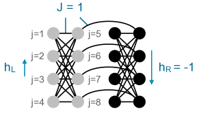
Figure 1: Graph of the problem Hamiltonian with 16 qubits coupled ferromagnetically with J=1 (lines). The applied fields are $0<h_{\rm L}<J/2$ ($h_{\rm R}=-1$) for the left (right) qubit cell. The symmetry and strong intra-cell ferromagnetic coupling makes each 8-qubit cluster evolve together.

The problem Hamiltonian encoding the computational primitive with one global minimum and one false minimum is depicted in Fig. 1. It consists of two qubit cells, left and right, each with $n=8$ qubits. The local fields $0<h_{\rm L}<0.5$ and $h_{\rm R}=-1$ are equal for all the spins within each cell, and all the couplings $J=1$ are ferromagnetic. The spins within each cell tend to move together as clusters due to symmetry and the strong intra-cell ferromagnetic coupling energy. We choose $|h_{\rm R}|>|h_{\rm L}|$, so that in the low energy states of $H_{P}$ the right cluster is pointing along its own local field as seen in Fig. 1. The difference in energy of the states with opposite polarization in the left cluster is $n(J-2h_{\rm L})$. Choosing $h_{\rm L}<J/2=0.5$, the global minimum corresponds to both clusters having the same orientation, while in the false minimum they have opposite orientations.

Our aim is to distinguish quantum tunneling from thermal activation along classical paths of product states (which preclude multiqubit tunneling). We now explain why a classical path continuously connects the initial global minimum to the final false minimum. At the beginning of the annealing process $B(s)/A(s)\ll 1$, and we have $\langle\sigma^{z}_{\mu}\rangle\simeq h_{k}\,B(s)/A(s)$ (because the coupling terms are quadratic in the z-polarizations $\langle\sigma^{z}_{\mu}\rangle$). As $h_{\rm L}$ and $h_{\rm R}$ have opposite signs, so will the z-projections of spins in the two clusters early in the evolution. To escape this path classically all spins in the left cluster must flip sign, which requires traversing an energy barrier. The barrier peak corresponds to zero total z-polarization of the left cluster. Therefore, the barrier grows with the ferromagnetic energy of the cluster $(n/2)^{2}J$. The barrier height is much greater than the residual energy which grows with $n(J-2h_{\rm L})$.

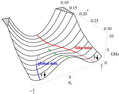
Figure 2: Energy potential using $h_{\rm L}=0.44$, plotted versus annealing $s$ and tilt angle $\theta_{\rm L}$ of each spin vector in the left cluster. The red line corresponds to a path that starts in the initial global minimum and follows the instantaneous local energy minimum. A second local minimum (dashed blue line) forms at the bifurcation point $s=0.18$. The global minimum is found in this second path after $s=0.24$ (dashed to continuous blue line). To reach this global minimum the system state has to traverse the energy barrier between them (dashed green line), either by thermal activation or by quantum tunneling.

In order to give a more precise description of the classical paths of product states, let each qubit be represented by a spin vector in the $xz$-plane. Denote by $\theta_{\mu}$ the angle of the spin vector for qubit $\mu$ with the $x$ quantization axis. We can gain an intuitive understanding of the effective energy landscape if we assume that all the qubits in the left (right) cluster have the same angle $\theta_{\rm L}$ ($\theta_{\rm R}$). This assumption is based on symmetry and the strong intra-cluster ferromagnetic energy. The resulting energy potential can be derived using more formal methods, like the Villain representation Boulatov and Smelyanskiy (2003). Figure 2 plots the effective energy potential for the left cluster as a function of $\theta_{\rm L}$ with $h_{\rm L}=0.44$. The classical path (red line) which follows the local minimum of this effective energy potential gets trapped in a false minimum and fails to solve the corresponding optimization problem, as explained in the previous paragraph.

In the absence of quantum tunneling, the global minimum could be reached through thermal excitations along classical paths for over-the-barrier escape from the false minimum. This thermal activation results in an increasing probability of success with rising temperature. This intuition is supported by spin vector Monte Carlo (SVMC), a numerical algorithm consisting in thermal Metropolis updates of the spin vectors Shin et al. (2014). Figure 5a confirms the thermal activation in SVMC. This is opposite to both open quantum system theory and experiments with the D-Wave chip, which show a reduction of the probability of success with rising temperature, as explained later. Furthermore, Figure 5b shows that the probability of success for SVMC is lower than the probability of success for D-Wave and open system quantum models.

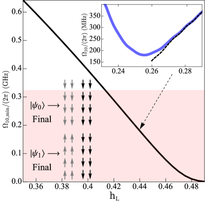
Figure 3: Inset shows the quantum energy gap $\hbar\Omega_{10}=E_{1}(s)-E_{0}(s)$ versus $s$, using $h_{\rm L}=0.44$. The dashed line is the gap in the diabatic (pointer) basis. In the main plot, the minimum gap decreases with $h_{\rm L}$. The horizontal boundary of the red-filled area (324 MHz) corresponds to 15.5 mK, the lowest temperature in our experiments. The lower inset shows the spin configurations of the two lowest eigenstates at the end of the annealing.

Quantum mechanically, the system evolution goes through an “avoided-crossing” where the two lowest eigenstates $E_{1}(s)$ and $E_{0}(s)$ approach closely to, and then repel from, each other (see inset in Fig. 3). Higher energy states remain well separated during the evolution. This level repulsion occurs due to the collective tunneling of qubits in the left cluster between the opposite $z$-polarizations. At the point where the gap $\hbar\Omega_{10}(s)$=$E_{1}(s)$-$E_{0}(s)$ reaches its minimum the corresponding adiabatic eigenstates are formed by the symmetric and anti-symmetric superpositions of the cluster orientations. The size of the minimum gap is varies with $h_{\rm L}$, as seen in Fig. 3.

Under realistic conditions, a quantum annealer can be strongly influenced by coupling to the environment, for which we introduce a detailed phenomenological open quantum system model. We shall assume that each flux qubit is coupled to its own environment with an independent noise source; this is consistent with experimental data Lanting et al. (2010). The coupling of the environment to each flux qubit is through flux fluctuations, and is proportional to a $\sigma^{z}$ qubit operator. The properties of the noise are determined by the noise spectral density $S(\omega)$, which is characterized by single-qubit macroscopic resonant tunneling (MRT) experiments in a broad range of biases (0.4 MHz $-$ 4 GHz) and temperatures (21 mK $-$ 38 mK) for tunneling amplitudes of a single flux qubit below 1 MHz . The MRT data collected is surprisingly well-described Harris et al. (2008); Lanting et al. (2011) by a phenomenological “hybrid” thermal noise model $S(\omega)=S_{\rm lf}(\omega)+S_{\rm oh}(\omega)$. Here $S_{\rm oh}(\omega)=\hbar^{2}\eta\omega e^{-\omega\tau_{c}}/(1-e^{-\hbar\omega/k_{B}T})$ denotes the high-frequency part, and has Ohmic form with dimensionless coupling $\eta$ and cutoff frequency $1/\tau_{c}$ (assumed to be very large). The low-frequency part $S_{\rm lf}$ is of the $1/f$ type Sendelbach et al. (2003) and in current D-Wave chips this noise is coupled to the flux qubit relatively strongly. Its effect can be described with only two parameters: the width $W$ and the Stokes shift $\epsilon_{p}$ of the MRT line Amin and Averin (2008). The experimental shift value is related to the width by the fluctuation-dissipation theorem ($\epsilon_{p}=\hbar W^{2}/2k_{B}T$) and represents the reorganization energy of the environment. The values of the noise parameters measured at the end of the annealing ($s=1$) for the D-Wave Two chip are $W/(2\pi)=0.40(1)\,{\rm GHz}$ and $\eta=0.24(3)$.

In the analysis of the transitions between the states we start from the initial (gapped) stage when the instantaneous energy gap $\hbar\Omega_{10}(s)$ between the two lowest eigenstates $|\psi_{0}(s)\rangle$, $|\psi_{1}(s)\rangle$ is sufficiently large compared to the linewidth $\hbar W$. Then the coupling to the environment can be treated as a perturbation and the transition rate between these states is then given by Fermi’s golden rule $\Gamma_{1\rightarrow 0}(s)\approx\mathbb{a}(s)S(\Omega_{10}(s))/\hbar^{2}$. Here

$$\mathbb{a}(s)=\sum_{\mu=1}^{2n}|\langle\psi_{0}(s)|\sigma_{\mu}^{z}|\psi_{1}(s)\rangle|^{2}$$ (3)

is a sum of (squared) transition matrix elements between the two eigenstates.

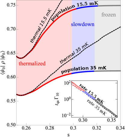
Figure 4: Solid lines correspond to the modeled population of the lowest energy eigenstate along the quantum annealing process using $h_{L}=0.44$ at 15.5 mK (top line) and 35 mK (bottom line). Dashed lines correspond to the thermal equilibrium population. In the thermalization phase (red) the transition rate is fast and the population remains close to thermal equilibrium. As the multiqubit energy barrier increases, the transition rates are exponentially reduced with $s$, as shown in the inset. We define the slowdown regime (blue) as $t_{qa}\Gamma_{1\rightarrow 0}<10$, and the frozen regime (gray) as $t_{qa}\Gamma_{1\rightarrow 0}<0.1$. Comparing the data at 15.5 and 35 mK, we see a small change in the transition rate relative to the larger change in the thermal equilibrium ground state population. Therefore, the probability of success is lower at higher temperature.

In the minimum gap region the (squared) matrix element $\mathbb{a}(s)$ for the transition rate is large, and the system is thermalized (see Fig. 4). More precisely, we have $\Gamma_{1\rightarrow 0}\gg 1/t_{qa}$, where the inverse of the annealing time $1/t_{qa}$ is an approximation for the annealing rate. The ground state population is given by the Boltzmann distribution at the experimental temperature.

After the avoided-crossing region we observe a steep exponential fall-off of the matrix element $\mathbb{a}(s)$ with $s$, eventually causing multiqubit freezing (see Fig. 4). Multiqubit freezing is quite distinct from single qubit freezing. Single qubit tunneling Johnson et al. (2011) decays slowly as the magnitude of the transverse field $A(s)$ decreases. The multiqubit transition rate, however, decays exponentially fast (see inset of Fig. 4). This is due to the increasing effective barrier width (see Fig. 2), which results in an exponential decrease of quantum tunneling and in a slowdown of the transition rate $\Gamma_{1\rightarrow 0}$. Formally, the barrier width corresponds to the Hamming distance

$$\mathbb{h}(s)=\sum_{\mu=1}^{2n}|\langle\psi_{0}|\sigma_{\mu}^{z}|\psi_{0}\rangle-\langle\psi_{1}|\sigma_{\mu}^{z}|\psi_{1}\rangle|^{2}/4$$ (4)

between the opposite $z$-orientations of the left cluster in the two lowest energy eigenstates. The exponential sensitivity of multiqubit tunneling to the width or Hamming distance $\mathbb{h}(s)$ is the cause of the exponential decay of the matrix element $\mathbb{a}(s)$, and of the multiqubit freezing.

We distinguish a slowdown phase (roughly $0.1<t_{qa}\Gamma_{1\rightarrow 0}<10$) and a frozen phase ($t_{qa}\Gamma_{1\rightarrow 0}<0.1$). In the frozen phase, there are no dynamics. Part of the system population remains trapped in the excited state $|\psi_{1}(s)\rangle$ corresponding to the false minimum of the effective potential until the end of the quantum annealing process (see Fig. 4).

The success probability of quantum annealing is (roughly) determined by the thermal equilibrium ground state population during the slowdown phase. When the temperature grows, the ground state population decreases appreciably, while the transition rate changes little (see Fig. 4). This results in the observed thermal reduction (see Fig. 5a).

When the energy gap is similar to (or smaller than) the noise linewidth $W$ the environment cannot be treated as a perturbation. We develop a multiqubit non-perturbative analysis in the spirit of the Non-interacting Blip Approximation (NIBA) Leggett et al. (1987) that covers all QA stages. In the slowdown phase, when the Hamming distance approaches its maximum value $\mathbb{h}\sim n$, the instantaneous decay rate of the first excited state takes the form

$$\Gamma_{1\rightarrow 0}=\int_{-\infty}^{\infty}d\tau\,e^{i\Omega_{10}\tau-\mathbb{h}(i\epsilon_{p}\tau+{(W\tau)^{2}}/{2})}\left[\frac{\pi\tau_{c}}{i\beta}{\rm csch}\frac{(\tau-i\tau_{c})}{\beta/\pi}\right]^{\frac{\mathbb{h}\eta}{2\pi}}D(\tau)\;,$$ (5)

where $1/\tau_{c}$ is the Ohmic noise cutoff frequency, $\beta$ is $\hbar/k_{B}T$, and the factor $D(\tau)$ is provided in Boixo et al. (2014b). The dependence on the annealing parameter $s$ is implicit. The factor $D(\tau)$ is related to the tunneling permeability of the potential barrier in Fig. 2 (similar to the coefficient $\mathbb{a}$). The above expression describes collective tunneling of the left qubit cluster assisted by the environment. The crucial difference from the single qubit MRT theory Amin and Averin (2008); Lanting et al. (2011) is that the parameters of the environment in the transition rate are rescaled by the barrier width or Hamming distance $\mathbb{h}(s)$. The effective low-frequency noise linewidth is $\mathbb{h}^{1/2}(s)W(s)$, the reconfiguration energy is $\mathbb{h}(s)\epsilon_{p}(s)$ and the Ohmic coefficient is $\mathbb{h}(s)\eta(s)$. This is important at the late stages of quantum annealing when $\mathbb{h}\sim n\gg 1$.

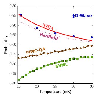
(a) Probability vs. temperature.

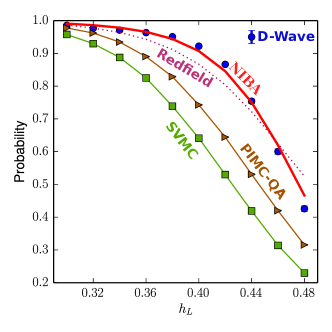
(b) Probability vs. $h_{\rm L}$.

Figure 5: Plots (a) and (b) show the probability of success for D-Wave (blue points) versus $h_{\rm L}$ and temperature. The decreasing probability with increasing temperature using $h_{L}=0.44$ is only matched with theories based on quantum tunneling. This is the opposite tendency to thermal activation (SVMC). Both Redfield and NIBA use only measured parameters (no fitting). In this temperature range the lowest two states (the double well potential) account for all the probability (0.9998 for D-Wave, 0.99998 for SVMC).

We observe a very close correspondence between the results of the analysis with the NIBA Quantum Master Equation for the dressed cluster states and the D-Wave Two data displayed in Fig. 5b. We emphasize that for NIBA (and the standard Redfield equation with $S_{\rm oh}(\omega)$) we do not have any parameter fitting: the parameters are obtained from MRT experiments, as explained above.

Figure 5a shows the success probability, as a function of temperature, for the D-Wave Two chip, open system quantum simulation and the classical-path model (SVMC) for $h_{\rm L}=0.44$. The D-Wave Two experimental data clearly shows thermal reduction: decreasing probability of success (ground state population) with temperature. This is a consequence of quantum tunneling, as seen in open quantum system theory. Contrary to the experimental data, SVMC shows thermal activation, with increasing success probability for increasing temperature. For a wide range of plausible parameters, only the quantum models show thermal reduction in these instances. The probability of success of SVMC is also lower than D-Wave Two data at the same temperature.

For $h_{\rm L}$ close to the degeneracy value $h_{\rm L}=J/2$ the minimum gap $\Omega_{10}^{\min}$ becomes small, as seen in Fig. 3. Where $\Omega_{10}\ll W$, the adiabatic basis of the instantaneous mutiqubit states $\{|\psi_{0}(s)\rangle$, $|\psi_{1}(s)\rangle\}$ loses its physical significance. Because the coupling to the bath is relatively strong here, the system quickly approaches the states corresponding to predominantly opposite cluster orientations, similar to diabatic states (see inset of Fig. 3). Transitions between these states, also called pointer states Zurek (1981), occur at a much slower rate as a consequence of the polaronic effect. As a result, for sufficiently small mininum gaps the multiqubit freezing starts before the avoided crossing and the success probability increases with temperature Dickson et al. (2013).

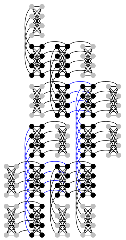
Figure 6: Larger problems that contain the tunneling probe “motif” as subproblems. As in Fig. 1, the black (grey) cluster has a strong $h_{R}=-1$ (weak $h_{L}=0.44$) local field. The black clusters are connected in a glassy fashion to make the problem less regular: all connections between any two neighboring black clusters are set randomly to either $-1$ or $+1$. The $-1$ connections are depicted in blue.

Figure 7: Success probability for a glass of clusters as a function of the number of qubits involved. We fit the mean probability of success $p(n_{q})\propto\exp(-\alpha n_{q})$ as a function of the number of qubits $n_{q}$ (dashed lines). The fitting exponent $\alpha$ for the D-Wave Two data is $(1.1\pm 0.05)\cdot 10^{-2}$, while the fitting exponent for PIMC-QA is $(2.2\pm 0.1)\cdot 10^{-2}$ and for the SVMC numerics is $(2.8\pm 0.17)\cdot 10^{-2}$. The error estimates for the exponents are obtained by bootstrapping.

A generalization of the 16 qubit problem to a larger number of qubits is achieved by studying problems that contain the same “motif” multiple times within the connectivity graph, see Fig. 6. The success probabilities for up to 200 qubits are shown in Fig. 7. We fit the average success probability as $p(n_{q})\propto\exp(-\alpha n_{q})$, where $n_{q}$ is the number of qubits. The fitting exponent $\alpha$ for the D-Wave Two data is $(1.1\pm 0.05)\cdot 10^{-2}$, while the fitting exponent for the SVMC numerics is $(2.8\pm 0.17)\cdot 10^{-2}$. We conclude that, for instances with multiqubit quantum tunneling, the D-Wave Two processor returns the solution that minimizes the energy with consistently higher probability than physically plausible models of the hardware that only employ product states and do not allow for multiqubit tunneling transitions.

The correlation between D-Wave’s experimental data and Path Integral Monte Carlo along the Quantum Annealing schedule (PIMC-QA) has been studied in recent works Boixo et al. (2014a); Rønnow et al. (2014); Albash et al. (2014). For completeness, we study PIMC-QA using similar parameters as in Boixo et al. (2014a). PIMC-QA gives a probability of success between SVMC and the quantum models (Figs. 5b and 7), and does not show thermal reduction for $h_{\rm L}=0.44$ (Fig. 5a).

A way to think of multiqubit tunneling as a computational resource is to regard it as a form of large neighborhood search. Collective tunneling transitions involving $K$ qubits explore a $K$ variable neighborhood, and there is a combinatorial number of such neighborhoods. We find that the current generation D-Wave Two annealer enables tunneling transitions involving at least 8 qubits. It will be an important future task to determine the maximal $K$ attainable by current technology and how large it can be made in next generations. The larger $K$, the easier it should be to translate the quantum resource “$K$-qubit tunneling” into a possible computational speedup. We want to emphasize that this paper does not claim to have established a quantum speedup. To this end one would have to demonstrate that no known classical algorithm finds the optimal solution as fast as the quantum process. To establish such an advantage it will be important to study to what degree collective tunneling can be emulated in classical algorithms such as Quantum Monte Carlo or by employing cluster update methods. However, the collective tunneling phenomena demonstrated here present an important step towards what we would like to call a physical speedup: a speedup relative to a hypothetical version of the hardware operated under the laws of classical physics.

Acknowledgments
We would like to thank John Martinis, Edward Farhi and Anthonty Leggett for useful discussions and reviewing the manuscript. We also thank Ryan Babbush and Bryan O’Gorman for reviewing the manuscript, and Damian Steiger, Daniel Lidar and Tameem Albash for comments about the temperature experiment. The work of V.N.S. was supported in part by the Office of the Director of National Intelligence (ODNI), Intelligence Advanced Research Projects Activity (IARPA), via IAA 145483 and by the AFRL Information Directorate under grant F4HBKC4162G001.

References

- Mohseni et al. (2014) M. Mohseni, Y. Omar, G. S. Engel, and M. B. Plenio, Quantum effects in biology (Cambridge University Press, 2014).
- Ray et al. (1989) P. Ray, B. K. Chakrabarti, and A. Chakrabarti, Phys. Rev. B 39, 11828 (1989).
- Finnila et al. (1994) A. B. Finnila, M. A. Gomez, C. Sebenik, C. Stenson, and J. D. Doll, Chem. Phys. Lett. 219, 343 (1994).
- Kadowaki and Nishimori (1998) T. Kadowaki and H. Nishimori, Phys. Rev. E 58, 5355 (1998).
- Brooke et al. (1999) J. Brooke, D. Bitko, T. F. Rosenbaum, and G. Aeppli, Science 284, 779 (1999).
- Farhi et al. (2002) E. Farhi, J. Goldstone, and S. Gutmann, arXiv:quant-ph/0201031 (2002).
- Santoro et al. (2002) G. E. Santoro, R. Martoňák, E. Tosatti, and R. Car, Science 295, 2427 (2002).
- Mooij et al. (1999) J. Mooij, T. Orlando, L. Levitov, L. Tian, C. H. Van der Wal, and S. Lloyd, Science 285, 1036 (1999).
- Harris et al. (2010) R. Harris, M. W. Johnson, T. Lanting, A. J. Berkley, J. Johansson, P. Bunyk, E. Tolkacheva, E. Ladizinsky, N. Ladizinsky, T. Oh, F. Cioata, I. Perminov, P. Spear, C. Enderud, C. Rich, S. Uchaikin, M. C. Thom, E. M. Chapple, J. Wang, B. Wilson, M. H. S. Amin, N. Dickson, K. Karimi, B. Macready, C. J. S. Truncik, and G. Rose, Phys. Rev. B 82, 024511 (2010).
- Lanting et al. (2010) T. Lanting, R. Harris, J. Johansson, M. H. S. Amin, A. J. Berkley, S. Gildert, M. W. Johnson, P. Bunyk, E. Tolkacheva, E. Ladizinsky, N. Ladizinsky, T. Oh, I. Perminov, E. M. Chapple, C. Enderud, C. Rich, B. Wilson, M. C. Thom, S. Uchaikin, and G. Rose, Phys. Rev. B 82, 060512 (2010).
- Johnson et al. (2011) M. Johnson, M. Amin, S. Gildert, T. Lanting, F. Hamze, N. Dickson, R. Harris, A. Berkley, J. Johansson, P. Bunyk, et al., Nature 473, 194 (2011).
- Boixo et al. (2013) S. Boixo, T. Albash, F. M. Spedalieri, N. Chancellor, and D. A. Lidar, Nat. Commun. 4 (2013).
- Dickson et al. (2013) N. Dickson, M. Johnson, M. Amin, R. Harris, F. Altomare, A. Berkley, P. Bunyk, J. Cai, E. Chapple, P. Chavez, et al., Nat. Commun. 4, 1903 (2013).
- McGeoch and Wang (2013) C. C. McGeoch and C. Wang, in Proceedings of the ACM International Conference on Computing Frontiers (ACM, 2013) p. 23.
- Boixo et al. (2014a) S. Boixo, T. F. Rønnow, S. V. Isakov, Z. Wang, D. Wecker, D. A. Lidar, J. M. Martinis, and M. Troyer, Nat. Phys. 10, 218 (2014a).
- Lanting et al. (2014) T. Lanting, A. Przybysz, A. Y. Smirnov, F. Spedalieri, M. Amin, A. Berkley, R. Harris, F. Altomare, S. Boixo, P. Bunyk, et al., Phys. Rev. X 4, 021041 (2014).
- Santra et al. (2014) S. Santra, G. Quiroz, G. Ver Steeg, and D. A. Lidar, New J. Phys. 16, 045006 (2014).
- Rønnow et al. (2014) T. F. Rønnow, Z. Wang, J. Job, S. Boixo, S. V. Isakov, D. Wecker, J. M. Martinis, D. A. Lidar, and M. Troyer, Science 345, 420 (2014).
- Vinci et al. (2014a) W. Vinci, K. Markström, S. Boixo, A. Roy, F. M. Spedalieri, P. A. Warburton, and S. Severini, Sci. Rep. 4 (2014a).
- Shin et al. (2014) S. W. Shin, G. Smith, J. A. Smolin, and U. Vazirani, arXiv:1401.7087 (2014).
- Vinci et al. (2014b) W. Vinci, T. Albash, A. Mishra, P. A. Warburton, and D. A. Lidar, arXiv:1403.4228 (2014b).
- Venturelli et al. (2014) D. Venturelli, S. Mandrà, S. Knysh, B. O’Gorman, R. Biswas, and V. Smelyanskiy, arXiv:1406.7553 (2014).
- Albash et al. (2014) T. Albash, T. F. Rønnow, M. Troyer, and D. A. Lidar, arXiv:1409.3827 (2014).
- Boixo et al. (2014b) S. Boixo, V. N. Smelyanskiy, A. Shabani, S. V. Isakov, M. Dykman, V. S. Denchev, M. Amin, A. Smirnov, M. Mohseni, and H. Neven, arXiv:1411.4036 (2014b).
- Boulatov and Smelyanskiy (2003) A. Boulatov and V. N. Smelyanskiy, Phys. Rev. A 68 (2003), 10.1103/PhysRevA.68.062321.
- Harris et al. (2008) R. Harris, M. Johnson, S. Han, A. Berkley, J. Johansson, P. Bunyk, E. Ladizinsky, S. Govorkov, M. Thom, S. Uchaikin, B. Bumble, A. Fung, A. Kaul, A. Kleinsasser, M. Amin, and D. Averin, Phys. Rev.Lett. 101, 117003 (2008).
- Lanting et al. (2011) T. Lanting, M. H. S. Amin, M. W. Johnson, F. Altomare, A. J. Berkley, S. Gildert, R. Harris, J. Johansson, P. Bunyk, E. Ladizinsky, E. Tolkacheva, and D. V. Averin, Phys. Rev. B 83, 180502 (2011).
- Sendelbach et al. (2003) S. Sendelbach, D. Hover, A. Kittel, M. Mück, J. M. Martinis, and R. McDermott, Phys. Rev. B 67, 094510 (2003).
- Amin and Averin (2008) M. H. S. Amin and D. V. Averin, Phys. Rev. Lett. 100, 197001 (2008).
- Leggett et al. (1987) A. J. Leggett, S. Chakravarty, A. T. Dorsey, M. P. A. Fisher, A. Garg, and W. Zwerger, Ref. Mod. Phys. 59, 1 (1987).
- Zurek (1981) W. H. Zurek, Phys. Rev. D 24, 1516 (1981).