The Observational Status of Cosmic Inflation after Planck

Abstract

The observational status of inflation after the Planck $2013$ and $2015$ results and the BICEP2/Keck Array and Planck joint analysis is discussed. These pedagogical lecture notes are intended to serve as a technical guide filling the gap between the theoretical articles on inflation and the experimental works on astrophysical and cosmological data. After a short discussion of the central tenets at the basis of inflation (negative self-gravitating pressure) and its experimental verifications, it reviews how the most recent Cosmic Microwave Background (CMB) anisotropy measurements constrain cosmic inflation. The fact that vanilla inflationary models are, so far, preferred by the observations is discussed and the reason why plateau-like potential versions of inflation are favored within this subclass of scenarios is explained. Finally, how well the future measurements, in particular of $B$-Mode CMB polarization or primordial gravity waves, will help to improve our knowledge about inflation is also investigated.

I Introduction

With the release of the Planck data $2013$ Ade et al. (2013a, b, c) and $2015$ Planck:2015xua (1343079); Ade et al. (2015a, b), and the recent BICEP2/Keck Array and Planck joint analysis BICEP2/Keck et al. (2015), the theory of cosmic inflation Starobinsky (1979, 1980); Guth (1981); Linde (1982); Mukhanov and Chibisov (1981, 1982); Starobinsky (1982) has acquired a new status. Several of its predictions such as spatial flatness of our Universe, the presence of Doppler peaks in the Cosmic Microwave Background (CMB) multipole moments, almost scale invariant power spectrum for density perturbations have been definitively confirmed by the recent CMB anisotropy measurements. That makes inflation a predictive and verified theory of the early Universe.

In fact, another remarkable outcome of the Planck data is that they also allow us to identify which version of inflation is most likely to have been realized in Nature Martin et al. (2014a, b); Martin (2013). As is well-known, inflation comes in different flavors but these different scenarios make different predictions and, thus, one can, at least in principle, distinguish among them. The fact that the primordial fluctuations are adiabatic and Gaussian to a relatively high degree of accuracy Ade et al. (2013b, c) is an important indication that we probably deal with single-field slow-roll inflation (with standard kinetic term), the simplest but non-trivial model of inflation. Of course, the final word has not yet been spoken since many non-vanilla inflationary scenarios are still compatible with the data. But, presently, they are just not needed in order to explain CMB measurements even if this situation could change in the future.

The fact that we now have high accuracy CMB data at our disposal also allows us to detect the “fine structure” of inflation and to constrain the shape of the inflaton potential. Here again, the Planck data have provided precious information. We now know that the potential is of the plateau type and that simple monomials are disfavored Ijjas et al. (2013); Martin et al. (2014a, b); Martin (2013). Moreover, we now start probing the reheating epoch Martin and Ringeval (2010); Martin et al. (2014c). Reheating is the epoch, after inflation and before the radiation dominated era of the standard hot Big bang phase, where the inflaton field decays and where all matter we see around us was produced Turner (1983); Traschen and Brandenberger (1990); Kofman et al. (1997); Amin et al. (2015). It is therefore of major conceptual importance. And Planck $2013$ and $2015$ data put non trivial constraints on the physical processes that took place at that time Martin and Ringeval (2006); Lorenz et al. (2008a); Martin and Ringeval (2010); Martin et al. (2014c); Munoz and Kamionkowski (2014); Dai et al. (2014); Gong et al. (2015).

The goal of these lectures, given at the second Jose Plinio Baptista school on Cosmology held in Pedra Azul (Brazil) in March $2014$, is to review how the above conclusions can be established. Many reviews on inflation can be found in the literature Martin (2004, 2005, 2008); Sriramkumar (2009) and there are technical papers reporting the astrophysical and cosmological observations, such as the Planck papers Ade et al. (2013a, b, c). But, in between, few things can be found and the present article aims at filling this gap. In some sense, it can be viewed as a technical guide which, from a reasonable prior knowledge of inflation, permits a detailed understanding of the implications for inflation of the recent high accuracy CMB data.

These lecture notes are also written at a special time: the Planck $2013$ and $2015$ data Ade et al. (2013a, b, c); Planck:2015xua (1343079); Ade et al. (2015a, b) have been released and their consequences (in fact, mainly the consequences of Planck $2013$) already analyzed in several works. Moreover, very recently, a joint analysis made by the BICEP2/Keck Array team and the Planck collaboration BICEP2/Keck et al. (2015) has been published showing that the BICEP2 detection of $B$-mode CMB polarization announced in Ref. Ade et al. (2014a) is mainly due to dust and cannot be attributed to primordial gravity waves produced during inflation. At the time of writing, the Planck $2015$ scientific products (in particular, the likelihood) are expected to be delivered in June $2015$ only. This means that reproducing or extending the Planck $2015$ analysis is not yet possible. However, from what is already known, the Planck $2015$ results are in good agreement with Planck $2013$. Therefore, the conclusions discussed in the present article (model comparison, constraints on reheating etc …) will most likely remain valid for the second release of the Planck data. Whenever available, we quote the values obtained by Planck $2015$.

These lectures are also related to the lectures given by C. Byrnes on Non-Gaussianities Byrnes (2014) and by D. Wands on CMB physics. Hopefully, these three reviews should provide the reader with a rather complete overview of modern primordial Cosmology and its observational implications. In particular, Ref. Byrnes (2014) reviews how Non-Gaussianities are produced in non-vanilla inflationary models while, here, we restrict ourselves to simple scenarios for which Non-Gaussianities are very small. The two lectures are therefore complementary. The lecture notes by D. Wands explain in details how CMB anisotropies are generated while, here, we just take it as a known fact (see also the recent review Bucher (2015)). Therefore, the present article and the one on CMB physics are also complementary.

These lecture notes are organized as follows. In the next section, Sec. II, we present general considerations on inflation. Rather than discussing inflation in detail, which can be found in many review articles, we just give the basics and choose to focus on the fundamental principles at the basis of the inflationary mechanism and its experimental justifications. In Sec. III, we discuss how inflation can be realized in practice. In particular, in Sec. III.1, we review how inflation can be embedded in high energy physics. Recently, alternative parametrizations have been considered and we discuss them in Sec. III.2. In Sec. III.3, we also review how the reheating phase can be described. Then, in Sec. IV, we discuss the theory of inflationary cosmological perturbations of quantum-mechanical origin. This part of the inflationary scenario is especially important because this is how one can relate theoretical predictions to astrophysical observations. In Sec. IV.1, we present the calculation of the two-point correlation functions, or power spectra, for scalar and tensor perturbations in the slow-roll approximation. In Sec. IV.2, we review the calculation of the three-point correlation function, or bispectrum, and in Sec. IV.3, the calculation of the four-point correlation function, or tri-spectrum. All these considerations are made in the slow-roll approximation and for single-field models with minimal kinetic terms. In Sec. IV.4, we discuss the isocurvature perturbations and how they can be produced in the framework of inflation. In Sec. V, we use the tools introduced before and compare the inflation predictions to the high accuracy CMB Planck data. In Sec. V.1, we consider the measurements of spatial curvature, in Sec. V.2 the measurements of isocurvature perturbations and, in Sec. V.3, those of Non-Gaussianities. Since these data indicate that single field models are preferred, we then focus on this class of scenarios. In Sec. V.4, we give the constraints on the slow-roll parameters and on the derived power-law parameters, such as the spectral index, the running or the tensor-to-scalar ratio. We also discuss the implications of the recent joint analysis made by the BICEP2/Keck Array team and the Planck collaboration. In Sec. V.5, we carry out a Bayesian analysis to do model comparison and determine what are the best models of inflation. In Sec. V.6, we present the constraints on reheating that can be inferred from the Planck data. Finally, in Sec. VI, we recap our main results and discuss which lesson can be drawn for our understanding of inflation and primordial cosmology.

II General Considerations on Inflation

The motivations for introducing a phase of inflation, i.e. a phase of accelerated expansion, are well-known: postulating $\ddot{a}>0$ ($a$ is the Friedmann-Lemaître-Roberston-Walker -FLRW- scale factor) allows us to avoid the puzzles of the standard hot Big Bang theory (for a detailed discussion of these issues, see Refs. Martin (2004); Mukhanov (2005); Peter and Uzan (2009)). If gravity is described by General Relativity (GR), then, in a homogeneous and isotropic Universe, the equations of motion are given by

$$H^{2}+\frac{{\cal K}}{a^{2}} = \left(\frac{\dot{a}}{a}\right)^{2}+\frac{{\cal K}}{a^{2}}=\frac{1}{3M_{\scriptscriptstyle{\mathrm{Pl}}}^{2}}\sum_{i}\rho_{i}\equiv\frac{1}{3M_{\scriptscriptstyle{\mathrm{Pl}}}^{2}}\rho,$$ (1.1)

$$-\left(2\frac{\ddot{a}}{a}+\frac{\dot{a}^{2}}{a^{2}}+\frac{{\cal K}}{a^{2}}\right) = \frac{1}{M_{\scriptscriptstyle{\mathrm{Pl}}}^{2}}\sum_{i}p_{i}\equiv\frac{1}{M_{\scriptscriptstyle{\mathrm{Pl}}}^{2}}p,$$ (1.2)

where $\rho_{i}$ and $p_{i}$ are respectively the energy density and the pressure of the fluid “$i$”. In the standard model of Cosmology, we have indeed a collection of different fluids, pressure-less matter (made of baryons and cold dark matter), radiation (made of photons and neutrinos) and dark energy. These different types of matter source the Einstein equations and control the dynamics of the expansion. Notice that the expansion rate of the Universe is given by the Hubble parameter which, according to the above equations, is defined by $H\equiv\dot{a}/a$ where a dot means a derivative with respect to cosmic time. The quantity $M_{\scriptscriptstyle{\mathrm{Pl}}}$ is the reduced Planck mass and, in the following, we will also use the quantity $\kappa\equiv 1/M_{\scriptscriptstyle{\mathrm{Pl}}}^{2}=8\pi G_{{}_{\rm N}}$, $G_{{}_{\rm N}}$ being the Newton constant. Finally, the quantity ${\cal K}$, that can always be normalized to $0$ or $\pm 1$, represents the curvature of the spatial sections. Notice that one can also define an effective curvature energy density by $\rho_{\rm curv}\equiv-3{\cal K}/(\kappa a^{2})$ such that the Friedmann equation takes the form $H^{2}=(\kappa/3)\sum_{i}\rho_{i}+(\kappa/3)\rho_{\rm curv}$. Defining $\Omega_{i}\equiv\rho/\rho_{\rm cri}$ and $\Omega_{\cal K}=\rho_{\rm curv}/\rho_{\rm cri}$, where the critical energy density is $\rho_{\rm cri}=3H^{2}/\kappa$, the Friedmann equation can be rewritten as $\sum_{i}\Omega_{i}+\Omega_{\cal K}=1$.

Let us now discuss under which physical conditions inflation can be obtained. The above equations can be combined and lead to the following formula which relates the acceleration of the expansion to the matter content of the Universe

$$\frac{\ddot{a}}{a}=-\frac{1}{6M_{\scriptscriptstyle{\mathrm{Pl}}}^{2}}\sum_{i}\left(\rho_{i}+3p_{i}\right)$$ (1.3)

This immediately implies that, in order to have inflation, the pressure must be negative, i.e. $p<-\rho/3$ where $\rho$ and $p$ are defined in Eqs. (1.1) and (1.2). Having realized that we need a negative pressure, the next question is of course which kind of matter can possess this property and this will be the subject of the two next sections. Of course, as is well-known, we will see that scalar fields are ideal candidates.

But before starting this discussion, it is interesting to notice that inflation is a genuine relativistic effect since it involves the term $3p$ in the above equation (1.3), which is absent in Newtonian physics. Indeed, let us consider a sphere of radius $R(t)$ and of uniform density $\rho$. A galaxy of mass $m$, located at the edge of the sphere, feels a gravitational field ${\bm{G}}$ that can be simply evaluated by means of the Gauss’s law, $\int{\bm{G}}\cdot{\rm d}{\bm{S}}=4\pi G_{{}_{\rm N}}M$, where $M$ is the mass of the sphere. This gives $G=G_{{}_{\rm N}}M/R^{2}$. As a consequence, the acceleration of the galaxy can be written as

$$m\ddot{R}=-m\frac{G_{{}_{\rm N}}M}{R^{2}},$$ (1.4)

or

$$\frac{\ddot{R}}{R}=-\frac{4\pi G_{{}_{\rm N}}}{3}\rho=-\frac{\rho}{6M_{\scriptscriptstyle{\mathrm{Pl}}}^{2}},$$ (1.5)

where we have used $M=4\pi\rho R^{3}/3$. This equation is similar to Eq. (1.3) except that the term $3p$ is not present. The physical reason behind the presence of this term is deeply rooted in the fundamental principles of GR: in GR, every form of energy weighs, including pressure.

The term $3p$ is so important for inflation that it is interesting to ask whether it plays a role in other physical situations and if its appearance has been tested experimentally and/or observationally. This is a difficult question since, in ordinary cases, the contribution of pressure is usually negligible, $p\ll\rho$. In fact, four situations where a gravitating pressure is important can be identified: inflation, dark energy but in some sense this is the same as inflation, neutron stars and Big Bang Nucleosynthesis (BBN). In particular, it is interesting to see what can be said about the $3p$ terms in the last two examples.

Let us start with the internal structure of a neutron star Schwab et al. (2008). As is well-known, it is controlled by the Tolman-Oppenheimer-Volkoff equations that can be obtained in the following way. The metric for a static and spherically symmetric solution can be written as

$${\rm d}s^{2}=-{\rm e}^{2\Phi}{\rm d}t^{2}+{\rm e}^{2\lambda}{\rm d}r^{2}+r^{2}\left({\rm d}\theta^{2}+\sin^{2}\theta{\rm d}\varphi^{2}\right),$$ (1.6)

where $t$ is time, $r$ a radial coordinate and $\theta$ and $\varphi$ angular coordinates. The quantities $\Phi$ and $\lambda$ are functions of $r$ only. Matter is assumed to be described by a perfect fluid, the stress energy tensor of which can be expressed as

$$T_{\mu\nu}=\left(\rho+p\right)u_{\mu}u_{\nu}+pg_{\mu\nu},$$ (1.7)

where $g_{\mu\nu}$ is the metric tensor and the normalized $4$-velocity reads $u_{\mu}=\left(-{\rm e}^{\Phi},0,0,0\right)$. Then, the time-time and $r-r$ component of the Einstein equations read

$$\frac{1}{r^{2}}{\rm e}^{-2\lambda}\left(2r\frac{{\rm d}\Phi}{{\rm d}r}+1-{\rm e}^{2\lambda}\right) = \frac{1}{M_{\scriptscriptstyle{\mathrm{Pl}}}^{2}}p,$$ (1.8)

$$\frac{1}{r^{2}}{\rm e}^{-2\lambda}\left(-1+2r\frac{{\rm d}\lambda}{{\rm d}r}+{\rm e}^{2\lambda}\right) = \frac{1}{M_{\scriptscriptstyle{\mathrm{Pl}}}^{2}}\rho.$$ (1.9)

On the other hand, energy conservation, $\nabla_{\mu}T^{\mu\nu}=0$, more precisely its radial component, implies that

$$\frac{{\rm d}p}{{\rm d}r}=-\left(\rho+p\right)\frac{{\rm d}\Phi}{{\rm d}r}.$$ (1.10)

The other components lead to the fact that $\rho$ does not depend on time, $\theta$ or $\varphi$, that is to say $\rho=\rho(r)$. If we now define the gravitational mass $m(r)$ by

$$G_{{}_{\rm N}}m(r)=\frac{r}{2}\left(1-{\rm e}^{-2\lambda}\right),$$ (1.11)

then Eq. (1.9) implies that

$$\frac{{\rm d}m}{{\rm d}r}=4\pi\rho(r)r^{2}.$$ (1.12)

Introducing the expression of the mass (1.11) in Eq. (1.8) in order to express ${\rm d}\Phi/{\rm d}r$ and, then, inserting the corresponding expression in the conservation equation (1.10) leads to

$$\frac{{\rm d}p}{{\rm d}r}=-(\rho+p)\frac{G_{{}_{\rm N}}}{r^{2}(1-2mG_{{}_{\rm N}}/r)}\left[m(r)+3p(r)\left(\frac{4}{3}\pi r^{3}\right)\right].$$ (1.13)

The important point in this formula is that the term $3p$ participates to this expression. This means that self-gravity of pressure affects the internal structure of the neutron stars. In practice, in order to calculate this internal structure, one has first to choose an equation of state $\rho=\rho(p)$. Once this is done, one can integrate the two following equations

$$\frac{{\rm d}\rho}{{\rm d}r}=\frac{{\rm d}\rho}{{\rm d}p}\frac{{\rm d}p}{{\rm d}r},\quad\frac{{\rm d}m}{{\rm d}r}=4\pi\rho(r)r^{2},$$ (1.14)

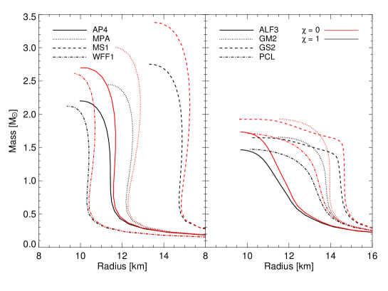
the last equation being nothing but Eq. (1.12). This leads to the functions $\rho(r)$ and $m(r)$. The radius of the star, $R_{\rm star}$, is defined by $\rho\left(R_{\rm star}\right)=0$ and its mass is given by $M_{\rm star}\equiv m\left(R_{\rm star}\right)$. One can then plot the mass-radius relation $M_{\rm star}(R_{\rm star})$. Of course, one obtains different mass-radius relations for different equations of state. Let us also notice that, at fixed equation of state, one obtains a curve, and not a unique prediction, because one needs to specify $\rho\left(r=0\right)$ to be able to integrate the above equations. One thus has a family of points parametrized by $\rho\left(r=0\right)$. Several examples are displayed in Fig. 1 (black lines).

Figure 1: Mass-radius relations of neutron stars for different equations of state (“standard” in the left panel, more “exotic” in the right panel). Black curves correspond to the standard GR calculation while red curves represent the case where self-gravity of pressure is absent. Figure taken from Ref. Schwab et al. (2008).

The fact that the structure of a neutron star depends on the general relativistic $3p$ term opens the possibility to experimentally test it. In order to do so, the idea of Ref. Schwab et al. (2008) is to study an ad-hoc modification of the Tolman-Openheimer-Volkoff equation such that

$$\frac{{\rm d}p}{{\rm d}r}=-(\rho+p)\frac{G_{{}_{\rm N}}}{r^{2}(1-2mG_{{}_{\rm N}}/r)}\left[m(r)+3\chi p(r)\left(\frac{4}{3}\pi r^{3}\right)\right],$$ (1.15)

where $\chi$ is a new, phenomenological, parameter introduced by hand. The term $3p$ weighs normally when $\chi=1$ and does not weigh at all when $\chi=0$. Notice that $\chi=0$ is not the Newtonian limit because there are other relativistic terms in Eq. (1.15) (for instance $1-2mG_{{}_{\rm N}}/r$ at the denominator). So the idea is now to re-derive the mass-radius relation for neutron stars and to see the influence of a parameter $\chi\neq 1$, the hope being to be able to put constraints on $\chi$ from astronomical observations. The results are shown in Fig. 1. The fact that red curves (namely those obtained with $\chi=0$) are different from the black ones (those obtained in the standard GR case) confirms that the $3p$ term has a significant influence of the mass-radius relation.

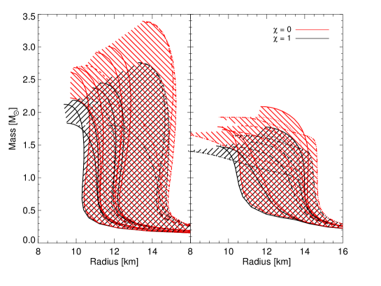
However, as shown in Fig. 2, the fact that the equation of state is not known accurately completely blurs the effect. Indeed, one sees that the corresponding uncertainty is typically of the same order of the effect we try to detect. Therefore, the conclusion is that, although it is true that self-gravity is crucial in order to predict correctly their mass-radius relation, at least for the moment, neutron stars cannot be used to experimentally test the $3p$ term.

Figure 2: Mass radius relations for different equations of state and associated theoretical uncertainties. In black are represented the mass radius relations obtained when $\chi=1$ (standard GR calculation) while, in red, are represented the mass radius relations obtained without self-gravity pressure (namely $\chi=0$). The hatched regions show the theoretical uncertainty associated with the fact that the equation of state is in fact unknown. It is clear from the plot that this completely dominates the differences between the $\chi=1$ and $\chi=0$ situations. Figure taken from Ref. Schwab et al. (2008).

Figure 3: Light elements abundances calculated when the Friedmann equation is modified according to Eq. (1.21). Greens contours are for deuterium abundance, blue ones for helium-$4$ and purple ones for lithium-$7$. The two gray ellipses indicate the region in parameter space allowed by observations. Figure taken from Ref. Rappaport et al. (2008).

Let us now turn to the other possibility, namely BBN Rappaport et al. (2008). Since BBN takes place during the radiation dominated era for which $p=\rho/3$, it is clear that the $3p$ term should have an important impact on BBN. In order test the influence of the $3p$ term, we follow the same strategy as for neutron stars and introduce an ad-hoc modification of GR characterized by the $\chi$ parameter, namely

$$\frac{\ddot{a}}{a}=-\frac{1}{6M_{\scriptscriptstyle{\mathrm{Pl}}}^{2}}(\rho+3\chi p).$$ (1.16)

This equation should be compared to Eq. (1.3). In order to derive the Friedmann equation, we need another equation and we can use the first law of thermodynamics for an adiabatic expansion, namely ${\rm d}(a^{3}\rho)=-p{\rm d}(a^{3})$, written for a co-moving volume or, equivalently, $\dot{\rho}+3\dot{a}(\rho+p)/a=0$. Then, noticing that $\ddot{a}/a=1/(2\dot{a}a){\rm d}(\dot{a}^{2})/{\rm d}t$ and using the conservation equation, it is straightforward to derive the following relation

$${\rm d}\left(\dot{a}^{2}\right)=-\frac{1}{3M_{\scriptscriptstyle{\mathrm{Pl}}}^{2}}\left[\left(1-3\chi\right)\rho a{\rm d}a-\chi a^{2}{\rm d}\rho\right].$$ (1.17)

If $\chi=1$, it is easy to check that

$${\rm d}\left(\dot{a}^{2}\right)=\frac{1}{3M_{\scriptscriptstyle{\mathrm{Pl}}}^{2}}{\rm d}\left(\rho a^{2}\right),$$ (1.18)

which gives

$$H^{2}=\frac{\rho}{3M_{\scriptscriptstyle{\mathrm{Pl}}}^{2}}+\frac{C}{a^{2}},$$ (1.19)

where $C$ is an integration constant leading to a curvature term. Now, if $\chi\neq 1$ and $p=w\rho$, where $w$ is a constant equation of state parameter, then one obtains

$$H^{2}=\frac{1+3\chi w}{1+3w}\frac{\rho}{3M_{\scriptscriptstyle{\mathrm{Pl}}}^{2}}+\frac{C}{a^{2}}.$$ (1.20)

Using this modified Friedmann equation with $w=1/3$ and ignoring the curvature term (which is sub-dominant in presence of radiation as shown by the cosmological data), one obtains

$$H^{2}=\frac{1+\chi}{2}\frac{\rho_{\rm rad}}{3M_{\scriptscriptstyle{\mathrm{Pl}}}^{2}}.$$ (1.21)

Therefore, the effect of the term proportional to $\chi$ is to modify the expansion rate of the Universe in the radiation dominated era. Or, if one uses the fact that the energy density of radiation is $\pi^{2}g_{*}T^{4}/30$, we see that this is also equivalent to changing the effective number of relativistic degrees of freedom, namely $g_{*}^{\prime}=g_{*}(1+\chi)/2$.

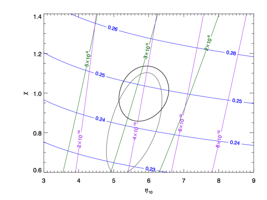
Ref. Rappaport et al. (2008) has performed BBN calculations, assuming Eq. (1.21), and computed the abundance of deuterium, helium-$4$ and lithium-$7$. The isocontours are represented in Fig. 3 in the plane $(\eta_{10},\chi)$. The parameter $\eta_{10}$ is defined by $\eta_{10}\equiv 10^{10}\eta$ where $\eta\equiv n_{{}_{\rm B}}/n_{\gamma}=\Omega_{{}_{\rm B}}h^{2}\pi^{2}\rho_{\rm cri}/[m_{{}_{\rm B}}h^{2}2T^{3}\zeta(3)]\simeq 2.73\times 10^{-8}\Omega_{{}_{\rm B}}h^{2}$ [in the last expression, $m_{{}_{\rm B}}\simeq 939.6\mbox{MeV}$ is the baryon (neutron) mass, $\rho_{\rm cri}\simeq 8.099\times 10^{-47}\mbox{GeV}^{4}$ is the critical energy density today, $T\simeq 2.7255\mbox{K}$ is the CMB temperature and $\zeta(3)\simeq 1.20206$]. Green contours represent the deuterium abundance $(D/H)_{{}_{\rm P}}$, blue contours are helium-$4$ abundance $Y_{{}_{\rm P}}$ and purple contours are lithium-$7$ abundance. We see that deuterium abundance mainly determines $\eta_{10}$ while helium-$4$ abundance gives good constraints on the new parameter $\chi$. Observations indicate that $\log\left(D/H\right)_{{}_{\rm P}}=-4.55\pm 0.04$ O’Meara et al. (2006) and $Y_{{}_{\rm P}}=0.24\pm 0.006$ Steigman (2007). Then, one can identify the region in the space $(\eta_{10},\chi)$ which is consistent with those observations. This is indicated in Fig. 3 by the two gray ellipses (corresponding to two slightly different assumptions about the abundances inferred from the observations). Without entering a detailed discussion, the conclusion is that $\chi\simeq 1$ is compatible with observations and that the value $\chi=0$ is strongly ruled out. Therefore, self-gravity of pressure is, in some sense, confirmed by cosmological observations.

The previous considerations “validate” the mechanism on which inflation is based. Inflation thus appears as a well-justified theory. In the next section, we therefore describe this theory in more detail and discuss the micro-physics of inflation.

III The Micro-Physics of Inflation or How to Parametrize Inflation

III.1 Inflation and High Energy Physics

We have seen in the last section that, in order to have a phase of inflation, we need a situation where the fluid dominating the matter content of the Universe has a negative pressure. The next question is of course which type of matter can have this property. In order to answer this question, let us first remark that inflation is a high energy phenomenon by particle physics standards since it is supposed to occur in the early Universe. In this situation, the relevant framework to describe matter is not fluid mechanics but field theory. And the simplest field, compatible with isotropy and homogeneity, is a time dependent scalar field $\phi(t)$ since it has no preferred direction and is space-independent. Moreover, in a FLRW Universe, the energy density and pressure of a scalar field are given by

$$\rho=\frac{\dot{\phi}^{2}}{2}+V(\phi),\quad p=\frac{\dot{\phi}^{2}}{2}-V(\phi).$$ (1.22)

As a consequence, in a situation where the potential energy dominates over the kinetic energy, namely when the field moves slowly or, equivalently, when the potential is flat, one obtains a negative pressure and, hence, inflation. The field which drives inflation is called the “inflaton”.

Let also notice that, when $V(\phi)\gg\dot{\phi}^{2}$, the equation of state is $p\simeq-\rho$ which, using the conservation equation, immediately implies that the energy density, and therefore the Hubble parameter $H$, is almost a constant. The Friedmann equation then leads to a scale factor $a(t)\propto{\rm e}^{Ht}$. In other words inflation is also a phase of quasi-exponential expansion. Moreover, using the expressions established above, one also has

$$|\Omega_{\cal K}|\equiv\left|\frac{\rho_{\rm curv}}{\rho_{\rm cri}}\right|=\frac{|{\cal K}|}{a^{2}H^{2}},$$ (1.23)

and we see that $\Omega_{\cal K}$ goes exponentially to zero during inflation. We therefore expect to measure a vanishing spatial curvature: this is a first generic prediction of inflation and we will see in Sec. V that it is good agreement with the most recent cosmological observations.

As mentioned before, inflation is a high energy phenomenon and, therefore, a concrete implementation necessarily rests on high energy physics. In the modern view, the micro-physics of inflation should therefore be described by an effective field theory characterized by a cutoff $\Lambda$. If the gravitational sector is described by GR, which itself is viewed as an effective theory with a cutoff at the Planck scale, then $\Lambda<M_{\scriptscriptstyle{\mathrm{Pl}}}$. On the other hand, we know that the Hubble parameter during the part of the inflationary phase we have observationally access to can be as large as $10^{15}\mathrm{GeV}$ and this suggests $\Lambda>10^{15}\mathrm{GeV}$. Clearly, at those energy scales, particle physics remains speculative and this is the reason why there is currently a plethora of different inflationary scenarios. A priori, without any further theoretical guidance, the effective action can therefore be written as

$$S = \int{\rm d}^{4}x\sqrt{-g}\biggl{[}M_{\scriptscriptstyle{\mathrm{Pl}}}^{2}\Lambda_{{}_{\rm B}}+\frac{M_{\scriptscriptstyle{\mathrm{Pl}}}^{2}}{2}R+aR^{2}+bR_{\mu\nu}R^{\mu\nu}+\frac{c}{M_{\scriptscriptstyle{\mathrm{Pl}}}^{2}}R^{3}+\cdots$$ (1.24)

$$-\frac{1}{2}\sum_{i}g^{\mu\nu}\partial_{\mu}\phi_{i}\partial_{\nu}\phi_{i}-V(\phi_{1},\cdots,\phi_{n})+\sum_{i}d_{i}\frac{{\cal O}_{i}}{\Lambda^{n_{i}-4}}\biggr{]}$$

$$+S_{\rm int}(\phi_{1},\cdots,\phi_{n},A_{\mu},\Psi)+\cdots$$

In the above equation, the first line represents the effective Lagrangian for gravity ($\Lambda_{{}_{\rm B}}$ is the cosmological constant). In practice, we will mainly work with the Einstein-Hilbert term only. The second line represents the contribution of matter. We assumed that several scalar field are present (a priori, there is no reason to assume that only one field plays a role). The two first terms are the canonical Lagrangian while ${\cal O}_{i}$ represents a higher order operator of dimension $n_{i}>4$, the amplitude of which is determined by the coefficient $d_{i}$. Those corrections can modify the potential but also the (standard) kinetic term Chialva and Mazumdar (2014). The last term encodes the interaction between the inflaton fields and the rest of the world, i.e. the gauge fields $A_{\mu}$ and the fermions $\Psi$. The dots stand for the rest of the terms such as the Lagrangians of $A_{\mu}$, of $\Psi$, the corresponding higher order operators etc … . Notice that the above description is not completely general. For instance, suppose that the action of the inflation field is of the Dirac-Born-Infeld (DBI) type Alishahiha et al. (2004), namely

$$S=\int{\rm d}^{4}x\sqrt{-g}\Biggl{[}\frac{M_{\scriptscriptstyle{\mathrm{Pl}}}^{2}}{2}R-T(\phi)\sqrt{1-2\frac{X}{T(\phi)}}+T(\phi)-V(\phi)\Biggr{]},$$ (1.25)

where $X\equiv-1/2g^{\mu\nu}\partial_{\mu}\phi\partial_{\nu}\phi$. An expansion in $X$ gives

$$S=\int{\rm d}^{4}x\sqrt{-g}\biggl{(}\frac{M_{\scriptscriptstyle{\mathrm{Pl}}}^{2}}{2}R-X+V+\frac{X^{2}}{2T(\phi)}+\cdots\biggr{)},$$ (1.26)

and we see that the higher order terms are not suppressed by a fixed cutoff $\Lambda$ but by $T(\phi)$. In this case, in some sense, the cutoff has become field dependent. As a consequence, the canonical Lagrangian $X-V$ is not necessarily always the first term of the series and it makes sense to also consider more complicated cases, even at “leading order”.

Another, but related, question is whether the higher order operators can be neglected during inflation. Firstly, it is necessary that the field excursion $\Delta\phi$ be small in comparison with the cutoff scale, i.e. $\Delta\phi<\Lambda$. Whether this is the case or not depends on the model. Second, the tree level potential $V$ can receive corrections that can be difficult to control. For instance, if there is a mass term, then typically the mass $m$ becomes

$$m^{2}\rightarrow m^{2}+gM^{2}\ln\left(\frac{\Lambda}{\mu}\right),$$ (1.27)

where $\mu$ is a renormalization scale, $M$ the mass of a heavy field and $g$ the coupling between $\phi$ and the heavy field. If $M>\Lambda$ then one has $m>H$ since we have $\Lambda>H$. This means that the potential is no longer flat enough to support inflation, an embarrassing problem indeed! Ways out consist in assuming that the coupling $g$ is small or, more convincingly, that symmetries forbid this type of corrections.

Finally, let us say a few words about the interaction term. Usually, it is considered to be negligible during the slow-roll phase. If this is not the case, it leads to warm inflation Berera (1995); Yokoyama and Linde (1999); Berera et al. (2009). Even if it does not play a role during the accelerated phase, the interaction term is of fundamental importance for inflation since it is responsible for the reheating stage, that is to say it explains how inflation is smoothly connected to the standard hot Big Bang epoch.

We see that, using theoretical considerations only, it is difficult to restrict the Lagrangian of inflation to a simple form. But, in fact, the point is that the CMB Planck data can do the job and can constrain the Lagrangian (1.24). For instance, we will see in the following that the perturbations are adiabatic (at least for the moment; this could of course very well change when more accurate data are collected) and this supports the idea that only one scalar field is at play during inflation. Moreover, we will also show that Non-Gaussianities have been measured to be compatible with zero and this supports the fact that the kinetic term must be standard. We are therefore led to consider that inflation is described by the simplest scenario, namely single-field slow-roll with a standard kinetic term. It is important to emphasize that we are pushed to this class of models, which is clearly easier to analyze than Eq. (1.24), not because we want to simplify the scenario but because this is what the CMB data suggest. In this framework, the inflationary Lagrangian can be written as

$$\mathcal{L}=-\frac{1}{2}g^{\mu\nu}\partial_{\mu}\phi\partial_{\nu}\phi-V(\phi)+\mathcal{L}_{\rm int}(\phi,A_{\mu},\Psi).$$ (1.28)

In the following, we will ignore the interaction term during the accelerated phase and will consider its effect only at the end of inflation (the “reheating” phase). We see that we are left with a model that contains only one arbitrary function, the potential $V(\phi)$. Therefore, what remains to be done in order to completely characterize inflation is to constrain this a priori arbitrary function with cosmological data. This line of research has played a dominant role in the recent years.

Let us now describe the slow-roll formalism which is used in practice to derive the inflationary predictions of the models mentioned above. As already remarked previously, one can distinguish two different phases of evolution: the slow-roll phase and the reheating phase. In principle, once $V(\phi)$ and $\mathcal{L}_{\rm int}(\phi,A_{\mu},\Psi)$ are known, the model is completely specified. In practice, however, one proceeds in a slightly different way. The function $V(\phi)$ is considered to be relevant for a limited range of field values only, corresponding to our observable window. Then, the evolution of the system is controlled by the Friedmann and Klein-Gordon equations, namely

$$H^{2} =\frac{1}{3M_{\scriptscriptstyle{\mathrm{Pl}}}^{2}}\left[\frac{\dot{\phi}^{2}}{2}+V(\phi)\right],$$ (1.29)

$$\ddot{\phi} +3H\dot{\phi}+V_{\phi}=0,$$ (1.30)

where we remind that $H\equiv\dot{a}/a$ denotes the Hubble parameter and where a subscript $\phi$ means a derivative with respect to the inflaton field. It is also interesting to introduce the Hubble flow functions $\epsilon_{n}$ defined by Schwarz et al. (2001); Leach et al. (2002)

$$\epsilon_{n+1}\equiv\frac{\mathrm{d}\ln\left|\epsilon_{n}\right|}{\mathrm{d}N},\quad n\geq 0,$$ (1.31)

where $\epsilon_{0}\equiv H_{\mathrm{ini}}/H$ starts the hierarchy and $N\equiv\ln(a/a_{\mathrm{ini}})$ is the number of e-folds. These parameters provide useful information about the inflationary dynamics. For instance, the first slow-roll parameter can be expressed as

$$\epsilon_{1}=-\frac{\dot{H}}{H^{2}}=1-\frac{\ddot{a}}{aH^{2}},$$ (1.32)

and, therefore, inflation ($\ddot{a}>0$) occurs if $\epsilon_{1}<1$. In fact, since the parameters $\epsilon_{n}$ are defined in terms of $H$ and since $H$ is determined once $V(\phi)$ is known, see Eqs. (1.29) and (1.30), it follows that one can also express them in terms of the potential. For instance, $\epsilon_{1}$ is given by

$$\epsilon_{1}=\frac{3\dot{\phi}^{2}}{2}\frac{1}{\dot{\phi}^{2}/2+V(\phi)}.$$ (1.33)

In fact, it is not sufficient to have $\epsilon_{1}<1$ but one also needs $\epsilon_{1}\ll 1$. Indeed, from the above expression, we see that this corresponds to a situation where $\dot{\phi}^{2}/2\ll V(\phi)$ or, in other words, to a situation where the potential is very flat since the field must roll very slowly. We just recover the case considered in the previous section. In this situation, referred to as the slow-roll approximation, one has in fact $\epsilon_{n}\ll 1$ for any $n$. If this is the case, then the Hubble flow functions can be expressed as Liddle et al. (1994)

$$\epsilon_{1} \simeq\frac{M_{\scriptscriptstyle{\mathrm{Pl}}}^{2}}{2}\left(\frac{V_{\phi}}{V}\right)^{2},$$ (1.34)

$$\epsilon_{2} \simeq 2M_{\scriptscriptstyle{\mathrm{Pl}}}^{2}\left[\left(\frac{V_{\phi}}{V}\right)^{2}-\frac{V_{\phi\phi}}{V}\right],$$ (1.35)

$$\epsilon_{2}\epsilon_{3} \simeq 2M_{\scriptscriptstyle{\mathrm{Pl}}}^{4}\left[\frac{V_{\phi\phi\phi}V_{\phi}}{V^{2}}-3\frac{V_{\phi\phi}}{V}\left(\frac{V_{\phi}}{V}\right)^{2}+2\left(\frac{V_{\phi}}{V}\right)^{4}\right].$$ (1.36)

The slow-roll approximation allows us to simplify the equations of motion and to analytically integrate the inflaton trajectory. Indeed, Eqs. (1.29) and (1.30), which control the evolution of $\phi$, can be rewritten as

$$H^{2} = \frac{V}{M_{\scriptscriptstyle{\mathrm{Pl}}}^{2}(3-\epsilon_{1})},$$ (1.37)

$$\left(1+\dfrac{\epsilon_{2}}{6-2\epsilon_{1}}\right)\dfrac{\mathrm{d}\phi}{\mathrm{d}N} = -M_{\scriptscriptstyle{\mathrm{Pl}}}^{2}\dfrac{\mathrm{d}\ln V}{\mathrm{d}\phi}\,.$$ (1.38)

As a consequence, in the slow-roll approximation, one has $H^{2}\simeq V/(3M_{\scriptscriptstyle{\mathrm{Pl}}}^{2})$ and ${\rm d}\phi/{\rm d}N\simeq-M_{\scriptscriptstyle{\mathrm{Pl}}}^{2}{\rm d}\ln V/{\rm d}\phi$, from which one obtains

$$N-N_{\mathrm{ini}}=-\frac{1}{M_{\scriptscriptstyle{\mathrm{Pl}}}^{2}}\int_{\phi_{\mathrm{ini}}}^{\phi}\frac{V(\chi)}{V_{\chi}(\chi)}\,\mathrm{d}\chi\,,$$ (1.39)

$\phi_{\mathrm{ini}}$ being the initial vacuum expectation value of the field. It is clear from the above considerations that the inflaton dynamics is entirely determined once the potential $V(\phi)$ has been specified. Since, in addition, the function $V(\phi)$ allows us to make the connection with high energy physics, it appears as a natural tool to parametrize inflation.

III.2 Other parametrizations?

Recently, other parametrizations of inflation have been considered. The motivation of these works was to establish a general framework in order to characterize what the generic or typical predictions of cosmic inflation are. In this section, we discuss them and show that, in fact, they all boil down to choosing a specific potential.

The first alternative parametrization that we discuss is the so-called “horizon-flow approach” Hoffman and Turner (2001); Kinney (2002); Liddle (2003); Ramirez and Liddle (2005); Chongchitnan and Efstathiou (2005). It has been recently discussed in detail in Ref. Vennin (2014). Let us define a new set of parameters ${}^{\ell}\lambda$ given by

$${}^{\ell}\lambda=\left(2M_{\scriptscriptstyle{\mathrm{Pl}}}^{2}\right)^{\ell}\frac{\left(H^{\prime}\right)^{\ell-1}}{H^{\ell}}\frac{{\rm d}^{\ell+1}H}{{\rm d}\phi^{\ell+1}}.$$ (1.40)

Of course, this new definition does not bring any new information. The new parameters can be expressed in terms of the previous ones, for instance ${}^{1}\lambda=\epsilon_{1}-\epsilon_{2}/2$, ${}^{2}\lambda=\epsilon_{1}^{2}-3\epsilon_{1}\epsilon_{2}/2+\epsilon_{2}\epsilon_{3}/2$, etc …. It only shows that, if the $\epsilon_{n}$’s are all of the same order in slow-roll, the ${}^{\ell}\lambda$ are of increasing order. Then, the simple equation, see Eq. (1.31)

$$\frac{{\rm d}\epsilon_{n}}{{\rm d}N}=\epsilon_{n}\epsilon_{n+1}$$ (1.41)

is replaced with

$$\frac{{\rm d}\epsilon_{1}}{{\rm d}N} = \epsilon_{1}\epsilon_{2},$$ (1.42)

$$\frac{{\rm d}\epsilon_{2}}{{\rm d}N} = 2{}^{2}\lambda-2\epsilon_{1}^{2}-3\epsilon_{1}\epsilon_{2},$$ (1.43)

$$\frac{{\rm d}{}^{\ell}\lambda}{{\rm d}N} = -{}^{\ell+1}\lambda-{}^{\ell}\lambda\left(\frac{\ell-1}{2}\epsilon_{2}-\epsilon_{1}\right).$$ (1.44)

The idea is now to truncate this hierarchy at some order $M$, i.e. to assume that ${}^{\ell}\lambda=0$ for $\ell>M$, maybe motivated by the fact that higher order equations deal with higher order slow-roll parameters and are thus, in some sense, negligible. Then, this finite set of equations (in practice, the case $M=5$ has been considered) is numerically integrated many times with different initial conditions Hoffman and Turner (2001). In this way, one obtains different values of the slow-roll parameters at Hubble radius crossing and, since the observables such as the spectral index $n_{\scriptscriptstyle{\mathrm{S}}}$ or the tensor-to-scalar ratio $r$ can be expressed in terms of these parameter (see below), different inflationary predictions. The next step consists in searching systematic patterns in these predictions which, as a consequence, would be considered as “typical” of inflation. In particular, it has been claimed that the different predictions for $n_{\scriptscriptstyle{\mathrm{S}}}$ and $r$ obtained in this way cluster around the relation Kinney (2002); Ramirez and Liddle (2005)

$$r_{16}\simeq\frac{1}{3}(1-n_{\scriptscriptstyle{\mathrm{S}}}),$$ (1.45)

where $r_{16}\equiv r/16$. The above equation is then viewed as a generic prediction of inflation, obtained without the need to specify a particular potential $V(\phi)$.

However, the above claim is not correct Vennin (2014). Indeed, truncating the hierarchy at order $M$ clearly means that one assumes, see Eq. (1.40),

$$\frac{{\rm d}^{M+2}H}{{\rm d}\phi^{M+2}}=0,$$ (1.46)

an equation which can be easily integrated (!) and leads to Liddle (2003)

$$H(\phi)=H_{0}\left[1+\sum_{i=1}^{M+1}A_{i}\left(\frac{\phi}{M_{\scriptscriptstyle{\mathrm{Pl}}}}\right)^{i}\right].$$ (1.47)

Then, from this expression of the Hubble parameter, one can easily calculate the corresponding inflationary potential and one obtains

$$V(\phi) = 3M_{\scriptscriptstyle{\mathrm{Pl}}}^{2}H^{2}(\phi)-2M_{\scriptscriptstyle{\mathrm{Pl}}}^{4}H^{\prime}(\phi)$$ (1.48)

$$= 3M_{\scriptscriptstyle{\mathrm{Pl}}}^{2}H_{0}^{2}\left[1+\sum_{i=1}^{M+1}A_{i}\left(\frac{\phi}{M_{\scriptscriptstyle{\mathrm{Pl}}}}\right)^{i}\right]^{2}-2M_{\scriptscriptstyle{\mathrm{Pl}}}^{3}H_{0}\sum_{i=1}^{M+1}iA_{i}\left(\frac{\phi}{M_{\scriptscriptstyle{\mathrm{Pl}}}}\right)^{i-1}.$$ (1.49)

The whole procedure is therefore nothing but a particular choice of a potential $V(\phi)$ depending on $M+1$ parameters, $A_{i}$. Moreover, Ref. Vennin (2014) has shown that the “mysterious” coefficient $1/3$ in Eq. (1.45) can be easily recovered if one carries out a standard slow-roll analysis of the potential (1.48). We conclude that this approach is not generic at all and only consists in studying a very particular potential.

More recently, it has also been argued that, rather than choosing a potential $V(\phi)$, it is more generic to choose the equation of state during inflation, see Refs. Mukhanov (2013); Binetruy et al. (2014); Mukhanov (2014). So, in practice, what is done is an educated guess for $w(N)=p/\rho$. Notice that, since

$$1+w(N)=\frac{2}{3}\epsilon_{1}(N),$$ (1.50)

this is also equivalent to choosing a particular function $\epsilon_{1}(N)$, which is the strategy followed in Refs. Roest (2014); Garcia-Bellido and Roest (2014); Binetruy et al. (2014). Concretely, one takes

$$1+w(N)=\frac{\beta}{\left(N_{\mathrm{end}}-N\right)^{\alpha}},$$ (1.51)

where $\alpha$ and $\beta$ are two free and positive parameters and $N_{\mathrm{end}}$ is the number of e-folds at the end of inflation. However, again, this choice is in fact a choice of $V(\phi)$. Indeed, the slow-roll trajectory (1.39), ${\rm d}N=-V{\rm d}\phi/(M_{\scriptscriptstyle{\mathrm{Pl}}}^{2}V^{\prime})$ can be re-written as

$$M_{\scriptscriptstyle{\mathrm{Pl}}}^{2}\frac{{\rm d}}{{\rm d}N}\left(\ln V\right)\simeq-\left(\frac{{\rm d}\phi}{{\rm d}N}\right)^{2},$$ (1.52)

and, from the exact formula

$$\epsilon_{1}=\frac{1}{2M_{\scriptscriptstyle{\mathrm{Pl}}}^{2}}\left(\frac{{\rm d}\phi}{{\rm d}N}\right)^{2},$$ (1.53)

one obtains the following system of equations

$$\left(\frac{{\rm d}\phi}{{\rm d}N}\right)^{2} = 3M_{\scriptscriptstyle{\mathrm{Pl}}}^{2}\left[1+w(N)\right],$$ (1.54)

$$\frac{{\rm d}}{{\rm d}N}\left(\ln V\right) = -3\left[1+w(N)\right].$$ (1.55)

When the above set of equations is solved one obtains $\phi(N)$ and $V(N)$ and, eventually eliminating $N$, the function $V(\phi)$. We conclude that giving $w(N)$ and/or $\epsilon_{1}(N)$ is not a new generic parametrization but just a particular choice of a potential. In order to illustrate this point, let us see how it works in practice for the case of Eq. (1.51). The trajectory, given by Eq. (1.54), can be written as

$$\frac{\phi}{M_{\scriptscriptstyle{\mathrm{Pl}}}}=C_{1}\pm\sqrt{3\beta}\frac{2}{\alpha-2}\left(N_{\mathrm{end}}-N\right)^{(2-\alpha)/2},$$ (1.56)

where $C_{1}$ is an integration constant. For the potential, the integration of Eq. (1.55) is also straightforward and one finds

$$\ln V=C_{2}+\frac{3\beta}{1-\alpha}\left(N_{\mathrm{end}}-N\right)^{1-\alpha},$$ (1.57)

where $C_{2}$ is another integration constant. Then, from Eq. (1.56), one arrives at

$$N_{\mathrm{end}}-N=\left[\pm\frac{\alpha-2}{2\sqrt{3\beta}}\left(\frac{\phi}{M_{\scriptscriptstyle{\mathrm{Pl}}}}-C_{1}\right)\right]^{2/(2-\alpha)},$$ (1.58)

and, inserting this result in Eq. (1.57), one obtains

$$\ln V=C_{2}+\frac{3\beta}{1-\alpha}\left[\pm\frac{\alpha-2}{2\sqrt{3\beta}}\left(\frac{\phi}{M_{\scriptscriptstyle{\mathrm{Pl}}}}-C_{1}\right)\right]^{2(1-\alpha)/(2-\alpha)}.$$ (1.59)

This shows that Eq. (1.51) is, in the slow-roll approximation, completely equivalent to the choice

$$V(\phi)=M^{4}{\rm e}^{\delta\phi^{\gamma}},$$ (1.60)

where $\delta$ and $\gamma$ are constants Mukhanov (2014). This potential is almost identical to Logamediate inflation, LMI in the terminology of Refs. Martin et al. (2014a, b), $V(\phi)=M^{4}x^{\alpha}{\rm e}^{\delta x^{\gamma}}$, with $x=(\phi-\phi_{0})/M_{\scriptscriptstyle{\mathrm{Pl}}}$, in the case where $\alpha=0$. This model was studied in detail in Refs. Martin et al. (2014a, b). The only difference is that, for LMI, one has $\alpha=4(1-\gamma)$ implying $\gamma=1$ when $\alpha=0$, which is not the case here (i.e. $\alpha=0$ but $\gamma$ is still free).

We conclude that all the so-called “alternative” parametrizations of inflation considered so far are in fact strictly equivalent to specifying a potential. Claiming that it is either new or different or better seems definitively far-fetched. In addition, discussing inflation in terms of $V(\phi)$ has the advantage to make the link with high energy physics explicit. For these reasons, we conclude that working in terms of $V(\phi)$ and scanning the inflationary landscape by considering all possible models seems to be the most efficient method to learn about inflation.

III.3 Parametrization of Reheating

Let us now consider the end of inflation, namely the reheating phase, and how one can describe it. When $\epsilon_{1}=1$, the potential is no longer flat enough to support an accelerated phase and inflation stops. Usually, this happens in the vicinity of the ground state (concretely, the minimum of the potential). At this time, the inflaton field starts oscillating and decaying. Then, these decay products thermalize Podolsky et al. (2006) and the radiation dominated epoch of the hot Big Bang phase commences. The micro-physics of reheating is described by the term $\mathcal{L}_{\rm int}(\phi,A_{\mu},\Psi)$ in Eq. (1.28). But, in fact, in order to parametrize reheating, we do not need to have such a detailed description. Indeed, as we will see in the following, the inflationary observational predictions are expressed in terms of $\epsilon_{n*}\equiv\epsilon_{n}(\phi_{*})$, where $\phi_{*}$ is the value of $\phi$ when the pivot scale $k_{{}_{\rm P}}$ leaves the Hubble radius during inflation (the pivot scale is conveniently chosen in the middle of the observable window). Since, in the slow-roll approximation, we know the trajectory $\phi=\phi(N)$, we just need to determine $N_{*}$ such that $\phi_{*}=\phi(N_{*})$. This can be done as follows. The physical pivot scale during inflation is given by

$$\frac{k_{{}_{\rm P}}}{a(N)}=\frac{k_{{}_{\rm P}}}{a_{\rm now}}\frac{a_{\rm now}}{a_{\rm reh}}\frac{a_{\rm reh}}{a_{\rm end}}\frac{a_{\rm end}}{a(N)}=\frac{k_{{}_{\rm P}}}{a_{\rm now}}\frac{a_{\rm now}}{a_{\rm reh}}\frac{a_{\rm reh}}{a_{\rm end}}{\rm e}^{N_{\mathrm{end}}-N},$$ (1.61)

where $a_{\rm end}$ denotes the scale factor at the end of inflation and $a_{\rm reh}$ the scale factor at the end of reheating. In the above expression, $k_{{}_{\rm P}}/a_{\rm now}$ is known and, concretely, we take $k_{{}_{\rm P}}/a_{\rm now}=0.05\mathrm{Mpc}^{-1}$. The quantity $a_{\rm now}/a_{\rm reh}$ is also known since it only involves the standard thermal history of the Universe. On the other hand, the ratio $a_{\rm reh}/a_{\rm end}$ depends on what happens during reheating and this is precisely the reason why the inflationary predictions are sensitive to this phase of evolution. To go further, we write the above equation at the time $N=N_{*}$. Since, by definition, $k_{{}_{\rm P}}/a(N_{*})=H(N_{*})$, Eq. (1.61) becomes

$$H(N_{*})=\frac{1}{M_{\scriptscriptstyle{\mathrm{Pl}}}}\sqrt{\frac{V(N_{*})}{3-\epsilon_{1}(N_{*})}}=\frac{k_{{}_{\rm P}}}{a_{\rm now}}\frac{a_{\rm now}}{a_{\rm reh}}\frac{a_{\rm reh}}{a_{\rm end}}{\rm e}^{N_{\mathrm{end}}-N_{*}},$$ (1.62)

the first expression being just the Friedmann equation, see Eq. (1.37). We see that this is a transcendental equation for $N_{*}$ which, therefore, needs to be solved numerically. We also see that it depends on the potential $V(\phi)$ and, hence, on the model under consideration. Finally, in order to solve this equation, one needs to estimate the quantity $a_{\rm reh}/a_{\rm end}$. Let $\rho$ and $p$ be the total energy density and pressure during reheating. Notice that one can have several fluids, possibly interacting which each others. The treatment presented here is therefore completely general. Conservation of total energy density (we emphasize again that it is not necessary to assume that the energy density of each fluid is separately conserved) implies that

$$\rho\left(N\right)=\rho_{\mathrm{end}}\exp\left\{-3\int_{N_{\mathrm{end}}}^{N}\left[1+w_{\mathrm{reh}}\left(n\right)\right]{\mathrm{d}}n\right\},$$ (1.63)

where $w_{\mathrm{reh}}\equiv p/\rho$ is the “instantaneous” equation of state during reheating. Then, let us define the mean equation of state parameter, $\overline{w}_{\mathrm{reh}}$, by

$$\overline{w}_{\mathrm{reh}}\equiv\frac{1}{\Delta N}\int_{N_{\mathrm{end}}}^{N_{\mathrm{reh}}}w_{\mathrm{reh}}(n)\mathrm{d}n,$$ (1.64)

where $\Delta N\equiv N_{\mathrm{reh}}-N_{\mathrm{end}}$ is the total number of e-folds during reheating. It follows that

$$\rho_{\rm reh}=\rho_{\rm end}{\rm e}^{-3(1+\overline{w}_{\mathrm{reh}})\Delta N},$$ (1.65)

and, therefore,

$${\rm e}^{\Delta N}=\frac{a_{\rm reh}}{a_{\rm end}}=\left(\frac{\rho_{\rm reh}}{\rho_{\rm end}}\right)^{-1/(3+3\overline{w}_{\mathrm{reh}})}.$$ (1.66)

As a consequence, the ratio $a_{\rm reh}/a_{\rm end}$ depends on two quantities only: the energy density at the end of reheating, $\rho_{\rm reh}$, and the mean equation of state during reheating, $\overline{w}_{\mathrm{reh}}$. Once a model of inflation is known, $\rho_{\rm end}$ can be calculated so this is not a new quantity (but, again, it introduces an additional dependence on the inflationary potential). Inserting Eq. (1.66) into the above expression (1.62) leads to

$$H(N_{*})=\frac{1}{M_{\scriptscriptstyle{\mathrm{Pl}}}}\sqrt{\frac{V(N_{*})}{3-\epsilon_{1}(N_{*})}}=\frac{k_{{}_{\rm P}}}{a_{\rm now}}\frac{a_{\rm now}}{a_{\rm reh}}\left(\frac{\rho_{\rm reh}}{\rho_{\rm end}}\right)^{-1/(3+3\overline{w}_{\mathrm{reh}})}{\rm e}^{N_{\mathrm{end}}-N_{*}}.$$ (1.67)

The above formula still contains $a_{\rm reh}$, a quantity that we would like to eliminate from the final expression. For this purpose, we write $a_{\rm now}/a_{\rm reh}$ as $a_{\rm now}/a_{\rm eq}\times a_{\rm eq}/a_{\rm reh}$, where $a_{\rm eq}$ is the scale factor at matter-radiation equality. Then, we use the fact that, during the radiation dominated era, $a\propto\rho^{-1/4}$, to write

$$H(N_{*}) = \frac{1}{M_{\scriptscriptstyle{\mathrm{Pl}}}}\sqrt{\frac{V(N_{*})}{3-\epsilon_{1}(N_{*})}}=\frac{k_{{}_{\rm P}}}{a_{\rm now}}\frac{a_{\rm now}}{a_{\rm eq}}\left(\frac{\rho_{\rm reh}}{\rho_{\rm eq}}\right)^{1/4}\left(\frac{\rho_{\rm reh}}{\rho_{\rm end}}\right)^{-1/(3+3\overline{w}_{\mathrm{reh}})}{\rm e}^{N_{\mathrm{end}}-N_{*}}$$ (1.69)

$$= \frac{k_{{}_{\rm P}}}{a_{\rm now}}\frac{a_{\rm now}}{a_{\rm eq}}\frac{M_{\scriptscriptstyle{\mathrm{Pl}}}}{\rho_{\rm eq}^{1/4}}\frac{\rho_{\rm end}^{1/2}}{M_{\scriptscriptstyle{\mathrm{Pl}}}^{2}}\frac{M_{\scriptscriptstyle{\mathrm{Pl}}}}{\rho_{\rm end}^{1/4}}\left(\frac{\rho_{\rm reh}}{\rho_{\rm end}}\right)^{1/4-1/(3+3\overline{w}_{\mathrm{reh}})}{\rm e}^{N_{\mathrm{end}}-N_{*}}.$$

Except the quantities that are known from standard cosmology (since they only depend on post-inflationary physics), such as $a_{\rm now}/a_{\rm eq}\times M_{\scriptscriptstyle{\mathrm{Pl}}}/\rho_{\rm eq}^{1/4}$, we see that this equation singles out the following combination (by definition, the “reheating” parameter) Martin and Ringeval (2006); Lorenz et al. (2008a); Martin and Ringeval (2010); Martin et al. (2014c)

$$R\equiv\frac{\rho_{\rm end}^{1/4}}{M_{\scriptscriptstyle{\mathrm{Pl}}}}R_{\mathrm{rad}},$$ (1.70)

with

$$R_{\mathrm{rad}}\equiv\left(\frac{\rho_{\rm reh}}{\rho_{\rm end}}\right)^{-1/4+1/(3+3\overline{w}_{\mathrm{reh}})}=\left(\frac{\rho_{\rm reh}}{\rho_{\rm end}}\right)^{(1-3\overline{w}_{\mathrm{reh}})/(12+12\overline{w}_{\mathrm{reh}})}.$$ (1.71)

Notice that we have a term $\rho_{\rm end}^{1/2}/M_{\scriptscriptstyle{\mathrm{Pl}}}^{2}$ left in Eq. (1.69). It is introduced because it produces a term proportional to the square root of the potential at the end of inflation and combines nicely with the $\sqrt{V_{*}}$ on the left hand side of Eq. (1.69). The arguments presented above can be easily generalized to take into account a change of relativistic degrees of freedom between the reheating epoch and today, see Ref. Martin et al. (2014a).

The reheating parameter encodes what can be learned about reheating from the CMB. In sec. V, we will see that the Planck data already put constraints on its value.

IV Inflationary perturbations

In this section, we review the theory of inflationary perturbations Mukhanov et al. (1992); Bardeen (1980); Peter (2013). This part of the inflationary scenario is very important because it allows us to use astrophysical data to put constraints on cosmic inflation. In the following, we pay special attention to the question of how one can calculate the correlation functions of the perturbations and to the concept of adiabatic and isocurvature perturbations. As will be seen in Sec. V, these quantities carry useful information about the type of inflationary model that is realized in Nature. This section can therefore be viewed as a preparation to Sec. V in the sense that we discuss in some detail the meaning of the quantities that have been measured recently by the Planck experiment.

To describe CMB anisotropies and large scale structures, one must go beyond the cosmological principle. This is a priori a technically difficult task but since the inhomogeneities are small in the early Universe, one can use a perturbative approximation which, obviously, greatly simplifies the problem. Then, the idea is to write the metric tensor as $g_{\mu\nu}(\eta,{\bm{x}})=g_{\mu\nu}^{{}_{\rm FLRW}}(\eta)+\delta g_{\mu\nu}(\eta,{\bm{x}})+\cdots$, where $g_{\mu\nu}^{{}_{\rm FLRW}}(\eta)$ represents the metric tensor of the FLRW Universe and where $\delta g_{\mu\nu}(\eta,{\bm{x}})\ll g_{\mu\nu}^{{}_{\rm FLRW}}(\eta)$. In fact, $\delta g_{\mu\nu}(\eta,{\bm{x}})$ can be expressed in terms of three types of perturbations, scalar, vector and tensor. In the context of inflation, only scalar and tensor are important. Scalar perturbations are directly coupled to the perturbed stress-energy tensor while tensor fluctuations are independent of $\delta T_{\mu\nu}$ and, in fact, are nothing but gravity waves. The equations of motion of each type of fluctuations are given by the perturbed Einstein equations, namely $\delta G_{\mu\nu}=\kappa\delta T_{\mu\nu}$.

In order to calculate the behavior of the fluctuations, we also need to specify the initial conditions. This is done by postulating that the perturbations are of quantum-mechanical origin and that, initially, their quantum state is the vacuum. This is possible because, at the beginning of inflation, the physical wavelengths of the Fourier modes of the perturbations are smaller than the Hubble radius. This means that, initially, space-time curvature is not felt and that, as a consequence, a well-motivated vacuum state can be defined.

IV.1 Inflationary two-point Correlation Functions

Once the equations of motion have been derived and the initial conditions specified, one can determine all the statistical properties of the fluctuations, in particular their two-point correlation functions or, in Fourier space, power spectra. The scalar perturbations are curvature perturbations defined by $\zeta(\eta,{\bm{x}})\equiv\Phi+2({\cal H}^{-1}\Phi^{\prime}+\Phi)/(3+3w)$, with $w=p/\rho$ the equation of state during inflation and $\Phi$ being the Bardeen potential Bardeen (1980) (not to be confused with the scalar field $\phi$). As usual in a linear theory, it is convenient to work in Fourier space and, therefore, we write

$$\zeta(\eta,{\bm{x}})=\frac{1}{(2\pi)^{3/2}}\int{\rm d}{\bm{k}}\,\zeta_{\bm{k}}(\eta)\,{\rm e}^{-i{\bm{k}}\cdot{\bm{x}}}.$$ (1.72)

As explained before, in the framework of the theory of cosmological perturbations of quantum-mechanical origin, the source of the perturbations is the unavoidable zero-point vacuum fluctuations. As a consequence, $\zeta(\eta,{\bm{x}})$ must in fact be viewed as a quantum operator and can be expressed as

$$\hat{\zeta}(\eta,{\bm{x}})=\int\frac{{\rm d}^{3}{\bm{k}}}{(2\pi)^{3/2}}\left[a_{\bm{k}}g_{\bm{k}}(\eta){\rm e}^{i{\bm{k}}\cdot{\bm{x}}}+a_{\bm{k}}^{\dagger}g_{\bm{k}}^{*}(\eta){\rm e}^{-i{\bm{k}}\cdot{\bm{x}}}\right],$$ (1.73)

where $a_{\bm{k}}$ and $a_{\bm{k}}^{\dagger}$ are respectively the annihilation and creation operators satisfying $[a_{\bm{k}},a_{\bm{p}}^{\dagger}]=\delta^{(3)}({\bm{k}}-{\bm{p}})$. The quantum state of the perturbations is the vacuum $|0\rangle$ which is, by definition, annihilated by the operator $a_{\bm{k}}$, namely $a_{\bm{k}}|0\rangle=0$. The function $g_{\bm{k}}(\eta)$ is the mode function and the Fourier transform of $\zeta(\eta,{\bm{x}})$ is given by $\zeta_{\bm{k}}(\eta)=a_{\bm{k}}g_{\bm{k}}(\eta)+a_{-{\bm{k}}}^{\dagger}g_{\bm{k}}^{*}(\eta)$. This last equation leads to $\langle 0|\zeta_{{\bm{k}}_{1}}\zeta_{{\bm{k}}_{2}}|0\rangle=|g_{{\bm{k}}_{1}}|^{2}\delta^{(3)}\left({\bm{k}}_{1}+{\bm{k}}_{2}\right)$. From the previous considerations, it follows that the two-point correlation function is given by

$$\langle\zeta^{2}(\eta,{\bm{x}})\rangle=\int\frac{{\rm d}k}{k}\mathcal{P}_{\zeta}(k)=\int\frac{{\rm d}k}{k}\frac{k^{3}}{2\pi^{2}}|g_{\bm{k}}|^{2},$$ (1.74)

where $\mathcal{P}_{\zeta}(k)$ is, by definition, the power spectrum of scalar perturbations. An exact calculation of this power spectrum is rarely available but a perturbative expansion into the slow-roll parameters (since they are small parameters) can be done and results in

$$\frac{\mathcal{P}_{\zeta}(k)}{\mathcal{P}_{\zeta 0}(k_{{}_{\rm P}})}=a_{0}^{{}_{({\rm S})}}+a_{1}^{{}_{({\rm S})}}\ln\left(\dfrac{k}{k_{{}_{\rm P}}}\right)+\frac{a_{2}^{{}_{({\rm S})}}}{2}\ln^{2}\left(\dfrac{k}{k_{{}_{\rm P}}}\right)+\dots\,,$$ (1.75)

where, as already mentioned, $k_{{}_{\rm P}}$ is the pivot scale and the overall amplitude can be written as

$$\mathcal{P}_{\zeta{{}_{0}}}=\frac{H_{*}^{2}}{8\pi^{2}\epsilon_{1*}M_{\scriptscriptstyle{\mathrm{Pl}}}^{2}}\,,$$ (1.76)

a star meaning that a quantity is evaluated at the time at which the pivot scale crossed out the Hubble radius during inflation. We see that the amplitude of the power spectrum depends on $H_{*}$ but also on the first slow-roll parameter, $\epsilon_{1*}$. The coefficients $a_{i}^{{}_{({\rm S})}}$ can be expressed in terms of the Hubble flow functions. For scalar perturbations, at second order in the slow-roll approximation, one gets Schwarz et al. (2001); Martin and Schwarz (2003); Casadio et al. (2005a, b, c); Gong and Stewart (2001); Choe et al. (2004); Leach et al. (2002); Lorenz et al. (2008b); Martin et al. (2013); Beltran Jimenez et al. (2013)

$$a_{0}^{{\scriptscriptstyle{(\mathrm{S})}}} = 1-2\left(C+1\right)\epsilon_{1*}-C\epsilon_{2*}+\left(2C^{2}+2C+\frac{\pi^{2}}{2}-5\right)\epsilon_{1*}^{2}$$ (1.77)

$$+ \left(C^{2}-C+\frac{7\pi^{2}}{12}-7\right)\epsilon_{1*}\epsilon_{2*}+\left(\frac{1}{2}C^{2}+\frac{\pi^{2}}{8}-1\right)\epsilon_{2*}^{2}$$

$$+ \left(-\frac{1}{2}C^{2}+\frac{\pi^{2}}{24}\right)\epsilon_{2*}\epsilon_{3*}+\cdots\,,$$

$$a_{1}^{{\scriptscriptstyle{(\mathrm{S})}}} = -2\epsilon_{1*}-\epsilon_{2*}+2(2C+1)\epsilon_{1*}^{2}+(2C-1)\epsilon_{1*}\epsilon_{2*}+C\epsilon_{2*}^{2}-C\epsilon_{2*}\epsilon_{3*}+\cdots\,,$$ (1.78)

$$a_{2}^{{\scriptscriptstyle{(\mathrm{S})}}} = 4\epsilon_{1*}^{2}+2\epsilon_{1*}\epsilon_{2*}+\epsilon_{2*}^{2}-\epsilon_{2*}\epsilon_{3*}+\cdots\,,$$ (1.79)

$$a_{3}^{{\scriptscriptstyle{(\mathrm{S})}}} = \mathcal{O}(\epsilon_{n*}^{3})\,,$$ (1.80)

where $C\equiv\gamma_{{\scriptscriptstyle{\mathrm{E}}}}+\ln 2-2\approx-0.7296$, $\gamma_{\scriptscriptstyle{\mathrm{E}}}$ being the Euler constant.

For tensor fluctuations, the approach is exactly similar to what we have just described. In particular, the tensor power spectrum $\mathcal{P}_{h}$ can be written in the same way as Eq. (1.75) but with a global amplitude now given by

$$\mathcal{P}_{h{{}_{0}}}=\frac{2H_{*}^{2}}{\pi^{2}M_{\scriptscriptstyle{\mathrm{Pl}}}^{2}}\,.$$ (1.81)

This time, the amplitude only depends on the Hubble parameter during inflation. Moreover, the coefficients $a_{i}^{{\scriptscriptstyle{(\mathrm{T})}}}$ have a similar structure and can be written as

$$a_{0}^{{\scriptscriptstyle{(\mathrm{T})}}} = 1-2\left(C+1\right)\epsilon_{1*}+\left(2C^{2}+2C+\frac{\pi^{2}}{2}-5\right)\epsilon_{1*}^{2}$$ (1.82)

$$+ \left(-C^{2}-2C+\frac{\pi^{2}}{12}-2\right)\epsilon_{1*}\epsilon_{2*}+\cdots\,,$$

$$a_{1}^{{\scriptscriptstyle{(\mathrm{T})}}} = -2\epsilon_{1*}+2(2C+1)\epsilon_{1*}^{2}-2(C+1)\epsilon_{1*}\epsilon_{2*}+\cdots\,,$$ (1.83)

$$a_{2}^{{\scriptscriptstyle{(\mathrm{T})}}} = 4\epsilon_{1*}^{2}-2\epsilon_{1*}\epsilon_{2*}+\cdots\,,$$ (1.84)

$$a_{3}^{{\scriptscriptstyle{(\mathrm{T})}}} = \mathcal{O}(\epsilon_{n*}^{3})\,.$$ (1.85)

The coefficients in front of the $\ln k$ term are related to the spectral indices and, at first order in the slow-roll parameters (we will discuss them in more detail in Sec. V), they can be expressed as

$$n_{\scriptscriptstyle{\mathrm{S}}}=1-2\epsilon_{1}-\epsilon_{2},\quad n_{\scriptscriptstyle{\mathrm{T}}}=-2\epsilon_{1},$$ (1.86)

where the first expression refers to scalar perturbations while the second is for tensor perturbations. Notice that, sometimes, the power spectrum is written as $k^{n_{\scriptscriptstyle{\mathrm{S}}}-1}$. In the context of slow-roll inflation, this is clearly not justified as it would amount to keep an infinite number of higher order terms while $n_{\scriptscriptstyle{\mathrm{S}}}$ has been evaluated at first order only. It is worth stressing that power-law power spectra are predictions of power-law inflation only, that is to say the inflationary model for which $V(\phi)\propto\exp(-C\phi)$ Lucchin and Matarrese (1985). From Eqs. (1.76) and (1.81), one can also estimate the relative contribution of tensor and scalar amplitudes

$$r\equiv\frac{\mathcal{P}_{h}}{\mathcal{P}_{\zeta}}=16\epsilon_{1*},$$ (1.87)

which means that, since $\epsilon_{1*}\ll 1$, tensor are sub-dominant. This is of course rather unfortunate since a direct measurement of gravity wave would directly lead to the energy scale during inflation, $H_{*}$.

IV.2 Inflationary three-point Correlation Functions

We have just derived the slow-roll inflationary two-point correlation functions but, of course, higher order correlation functions are also interesting and the field of Non-Gaussianity has played an important role in the recent years, see Refs. Gangui et al. (1994); Gangui (1994); Wang and Kamionkowski (2000); Gangui and Martin (2000a, b); Gangui et al. (2002) for original works on this question and Refs. Maldacena (2003); Seery and Lidsey (2005); Chen et al. (2007); Hotchkiss and Sarkar (2010); Chen (2010); Martin and Sriramkumar (2012); Hazra et al. (2012, 2013); Sreenath et al. (2013); Martin et al. (2014d); Sreenath and Sriramkumar (2014); Sreenath et al. (2014) for later works. For a complete overview of the subject, we refer to the lecture notes by C. Byrnes Byrnes (2014). Here, in order to be able to fully appreciate the relevance of the Planck data on Non-Gaussianities, we discuss how the three-point inflationary correlation functions can be calculated in the case of single-field slow-roll inflation with a minimal kinetic term.

For the two-point correlation, we have seen that it is convenient to work in Fourier space and to define the power spectrum. In the same way, for the three-point correlation function, we can define the bispectrum as a correlator in Fourier space, namely $\langle\zeta_{{\bm{k}}_{1}}(\eta)\,\zeta_{{\bm{k}}_{2}}(\eta)\,\zeta_{{\bm{k}}_{3}}(\eta)\rangle$. In fact, we will rather calculate the quantity $\langle{\mathcal{R}}_{{\bm{k}}_{1}}(\eta)\,{\mathcal{R}}_{{\bm{k}}_{2}}(\eta)\,{\mathcal{R}}_{{\bm{k}}_{3}}(\eta)\rangle$ where ${\mathcal{R}}\equiv-\Psi-{\cal H}\delta\phi^{\rm(gi)}/\phi^{\prime}$, $\Psi=\Phi$ (valid if a scalar field dominates the matter content of the Universe) being another Bardeen potential and $\delta\phi^{\rm(gi)}$ being the gauge invariant scalar field fluctuation Mukhanov et al. (1992). This amounts to a simple change of sign of the three-point function (and no change at the power spectrum level, namely $\mathcal{P}_{\zeta}=\mathcal{P}_{{\mathcal{R}}}$, because the power spectrum is quadratic in the Fourier amplitudes) since ${\mathcal{R}}=-\zeta$. Concretely one has

$$\langle{{\mathcal{R}}}(\eta,{\bm{x}})\,{{\mathcal{R}}}(\eta,{\bm{x}})\,{{\mathcal{R}}}(\eta,{\bm{x}})\rangle= \int\frac{{\rm d}^{3}{\bm{k}}_{1}}{(2\,\pi)^{3/2}}\;\int\!\frac{{\rm d}^{3}{\bm{k}}_{2}}{(2\,\pi)^{3/2}}\;\int\frac{{\rm d}^{3}{\bm{k}}_{3}}{(2\,\pi)^{3/2}}\;\langle{\mathcal{R}}_{{\bm{k}}_{1}}(\eta)\,{\mathcal{R}}_{{\bm{k}}_{2}}(\eta)\,{\mathcal{R}}_{{\bm{k}}_{3}}(\eta)\rangle\;$$

$$\times{\rm e}^{i\,\left({\bm{k}}_{1}+{\bm{k}}_{2}+{\bm{k}}_{3}\right)\cdot{\bm{x}}}.$$ (1.91)

In the above expression ${\mathcal{R}}_{{\bm{k}}}(\eta)$ obviously represents the Fourier transform of the curvature (scalar) perturbation ${\mathcal{R}}(\eta,{\bm{x}})$, namely

$${\mathcal{R}}(\eta,{\bm{x}})=\frac{1}{(2\pi)^{3/2}}\int{\rm d}{\bm{k}}\,{\mathcal{R}}_{\bm{k}}(\eta)\,{\rm e}^{-i{\bm{k}}\cdot{\bm{x}}}.$$ (1.92)

As explained before, in the framework of the theory of cosmological perturbations of quantum-mechanical origin, it is an operator and it can be expressed as

$$\hat{{\mathcal{R}}}(\eta,{\bm{x}})=\int\frac{{\rm d}^{3}{\bm{k}}}{(2\pi)^{3/2}}\left[a_{\bm{k}}f_{\bm{k}}(\eta){\rm e}^{i{\bm{k}}\cdot{\bm{x}}}+a_{\bm{k}}^{\dagger}f_{\bm{k}}^{*}(\eta){\rm e}^{-i{\bm{k}}\cdot{\bm{x}}}\right],$$ (1.93)

leading to $\langle{\mathcal{R}}_{{\bm{k}}_{1}}{\mathcal{R}}_{{\bm{k}}_{2}}\rangle=|f_{{\bm{k}}_{1}}|^{2}\delta^{(3)}\left({\bm{k}}_{1}+{\bm{k}}_{2}\right)$ since ${\mathcal{R}}_{\bm{k}}=a_{\bm{k}}f_{\bm{k}}+a_{-{\bm{k}}}^{\dagger}f_{\bm{k}}^{*}$. Here, the creation and annihilation operators are the same as those appearing in Eq. (1.73). Of course working in terms of ${\mathcal{R}}_{\bm{k}}(\eta)$ instead of $\zeta_{\bm{k}}(\eta)$ is both harmless and trivial since ${\mathcal{R}}_{\bm{k}}=-\zeta_{\bm{k}}$ and $f_{\bm{k}}(\eta)=-g_{\bm{k}}(\eta)$! We do it since many papers on Non-Gaussianities use this variable.

At this stage, it may be useful to say a few words about conventions. In this article, we are using Fourier transforms as defined in Eq. (1.92). Another convention, often used in the literature on Non-Gaussianities, is

$${\mathcal{R}}(\eta,{\bm{x}})=\frac{1}{(2\pi)^{3}}\int{\rm d}{\bm{k}}\,\bar{{\mathcal{R}}}_{\bm{k}}\,{\rm e}^{-i{\bm{k}}\cdot{\bm{x}}},$$ (1.94)

so that $\bar{{\mathcal{R}}}_{\bm{k}}=(2\pi)^{3/2}{\mathcal{R}}_{\bm{k}}$. This implies that $\langle\bar{{\mathcal{R}}}_{{\bm{k}}_{1}}\bar{{\mathcal{R}}}_{{\bm{k}}_{2}}\rangle=(2\pi)^{3}|f_{{\bm{k}}_{1}}|^{2}\delta^{(3)}\left({\bm{k}}_{1}+{\bm{k}}_{2}\right)$. Notice that the two-point correlation function is sometimes defined as $\langle\bar{{\mathcal{R}}}_{{\bm{k}}_{1}}\bar{{\mathcal{R}}}_{{\bm{k}}_{2}}\rangle\equiv(2\pi)^{3}P_{{\mathcal{R}}}(k_{1})\delta^{(3)}\left({\bm{k}}_{1}+{\bm{k}}_{2}\right)$ which leads to the identification $P_{{\mathcal{R}}}(k_{1})=|f_{{\bm{k}}_{1}}|^{2}$ [the quantity $P_{{\mathcal{R}}}(k_{1})$ should not be confused with $\mathcal{P}_{{\mathcal{R}}}(k_{1})=k_{1}^{3}|f_{{\bm{k}}_{1}}|^{2}/(2\pi^{2})]$. These definitions imply that $\bar{{\mathcal{R}}}_{\bm{k}}=(2\pi)^{3/2}\left(a_{\bm{k}}f_{\bm{k}}+a_{-{\bm{k}}}^{\dagger}f_{\bm{k}}^{*}\right)$ which can be rewritten as $\bar{{\mathcal{R}}}_{\bm{k}}=\bar{a}_{\bm{k}}f_{\bm{k}}+\bar{a}_{-{\bm{k}}}^{\dagger}f_{\bm{k}}^{*}$ with $\bar{a}_{\bm{k}}=(2\pi)^{3/2}a_{\bm{k}}$. In particular, since $[a_{\bm{k}},a_{\bm{p}}^{\dagger}]=\delta^{(3)}\left({\bm{k}}-{\bm{p}}\right)$, we now have $[\bar{a}_{\bm{k}},\bar{a}_{\bm{p}}^{\dagger}]=(2\pi)^{3}\delta^{(3)}\left({\bm{k}}-{\bm{p}}\right)$. Different conventions basically correspond to different choices for where the factors $2\pi$ appear in the equations. In principle straightforward, it can sometimes be confusing when one tries to check a result in the existing literature.

The bispectrum can be evaluated using the standard rules of quantum field theory. It is given by Maldacena (2003); Seery and Lidsey (2005)

$$\langle{\mathcal{R}}_{{\bm{k}}_{1}}(\eta)\,{\mathcal{R}}_{{\bm{k}}_{2}}(\eta)\,{\mathcal{R}}_{{\bm{k}}_{3}}(\eta)\rangle=-i\int_{\eta_{\rm ini}}^{\eta_{\rm e}}{\rm d}\tau\,a(\tau)\left\langle\left[{\mathcal{R}}_{{\bm{k}}_{1}}(\eta)\,{\mathcal{R}}_{{\bm{k}}_{2}}(\eta)\,{\mathcal{R}}_{{\bm{k}}_{3}}(\eta),H_{\rm int}(\tau)\right]\right\rangle,$$

where $\eta_{\rm ini}$ represents an initial time at the beginning of inflation (in practice we take $\eta_{\rm ini}\rightarrow-\infty$) and $\eta_{\rm e}$ a final time at the end of inflation when all the scales relevant to the problem are outside the Hubble radius (in practice we take $\eta_{\rm e}\rightarrow 0$). The quantity $H_{\rm int}$ is the interaction Hamiltonian. It can be obtained from the action of the system expanded up to third order in ${\mathcal{R}}$, the action of the system being the Einstein-Hilbert action plus that of a scalar field (the inflaton). A now standard calculation gives Maldacena (2003); Seery and Lidsey (2005); Chen et al. (2007); Chen (2010)

$${\cal S}_{3}[{\mathcal{R}}]=M_{\scriptscriptstyle{\mathrm{Pl}}}^{2}\int{\rm d}t\;{\rm d}^{3}{\bm{x}}\;\Biggl{[}a^{3}\,\epsilon_{1}^{2}\,{{\mathcal{R}}}\,{\dot{{\mathcal{R}}}}^{2}+a\,\epsilon_{1}^{2}\,{{\mathcal{R}}}\,({\partial}{{\mathcal{R}}})^{2}-2\,a\,\epsilon_{1}\,{\dot{{\mathcal{R}}}}\,({\partial}^{i}{{\mathcal{R}}})\,({\partial}_{i}\chi)$$ (1.96)

$$+ \frac{a^{3}}{2}\,\epsilon_{1}\,{\dot{\epsilon}_{2}}\,{{\mathcal{R}}}^{2}\,\dot{{\mathcal{R}}}+\frac{\epsilon_{1}}{2a}\,(\partial^{i}{\mathcal{R}})\,({\partial}_{i}\chi)\,({\partial}^{2}\chi)+\frac{\epsilon_{1}}{4\,a}\,({\partial}^{2}{{\mathcal{R}}})\,({\partial}\chi)^{2}+{\cal F}\left(\frac{\delta{\cal L}_{2}}{\delta{\mathcal{R}}}\right)\Biggr{]},$$

where $\delta{\cal L}_{2}/\delta{\mathcal{R}}$ denotes the variation of the second order action with respect to ${\mathcal{R}}$, and is given by

$$\frac{\delta{\cal L}_{2}}{\delta{\mathcal{R}}}={\dot{\Lambda}}+H\,\Lambda-\epsilon_{1}\,\partial^{2}{\mathcal{R}},$$ (1.97)

and the quantities $\Lambda$ and $\chi$ are defined by

$$\Lambda\equiv\frac{a^{2}\dot{\phi}^{2}}{2M_{\scriptscriptstyle{\mathrm{Pl}}}^{2}H^{2}}\dot{\mathcal{R}}=a^{2}\epsilon_{1}\dot{\mathcal{R}},\quad\chi\equiv\partial^{-2}\Lambda.$$ (1.98)

The term ${\cal F}(\delta{\cal L}_{2}/\delta{\mathcal{R}})$ introduced in Eq. (1.96) stands for the following complicated expression

$${\cal F}\left(\frac{\delta{\cal L}_{2}}{\delta{\mathcal{R}}}\right) = \frac{a}{2}\epsilon_{2}\left(\frac{\delta{\cal L}_{2}}{\delta{\mathcal{R}}}\right){\mathcal{R}}^{2}+\frac{2a}{H}\left(\frac{\delta{\cal L}_{2}}{\delta{\mathcal{R}}}\right)\dot{\mathcal{R}}{\mathcal{R}}$$

$$+ \frac{1}{2aH}\Biggl{\{}(\partial^{i}{\mathcal{R}})\;({\partial}_{i}\chi)\,\left(\frac{\delta{\cal L}_{2}}{\delta{\mathcal{R}}}\right)+\,\delta^{ij}\,\left[\Lambda\,({\partial}_{i}{\mathcal{R}})+({\partial}^{2}{\mathcal{R}})\,({\partial}_{i}\chi)\right]\,$$

$$\times {\partial}_{j}\left[{\partial}^{-2}\left(\frac{\delta{\cal L}_{2}}{\delta{\mathcal{R}}}\right)\right]+\frac{\delta^{im}\delta^{jn}}{H}({\partial}_{i}{\mathcal{R}})\,({\partial}_{j}{\mathcal{R}})\;{\partial}_{m}{\partial}_{n}\left[{\partial}^{-2}\left(\frac{\delta{\cal L}_{2}}{\delta{\mathcal{R}}}\right)\right]\Biggr{\}}.$$

The terms which involves $\delta{\cal L}_{2}/\delta{\mathcal{R}}$ can be removed by a suitable field redefinition of ${\mathcal{R}}$ of the following form Maldacena (2003); Seery and Lidsey (2005); Chen et al. (2007); Chen (2010):

$${\mathcal{R}}\rightarrow{\mathcal{R}}_{n}+\epsilon_{2}\frac{{\mathcal{R}}_{n}^{2}}{4}.$$ (1.100)

After this redefinition, the perturbed action (1.96) becomes a functional of ${\mathcal{R}}_{n}$. In the following, in order to avoid too complicated notations, we will still use ${\mathcal{R}}$ in place of ${\mathcal{R}}_{n}$. Then, with the redefinition (1.100), the interaction Hamiltonian can be expressed as

$$H_{\rm int}(\eta) = -M_{\scriptscriptstyle{\mathrm{Pl}}}^{2}\int{\rm d}^{3}{\bm{x}}\;\biggl{[}a\,\epsilon_{1}^{2}\,{\mathcal{R}}\,{\mathcal{R}}^{\prime 2}+a\,\epsilon_{1}^{2}\,{\mathcal{R}}\,({\partial}{\mathcal{R}})^{2}-2\,\epsilon_{1}\,{\mathcal{R}}^{\prime}\,({\partial}^{i}{\mathcal{R}})\,({\partial}_{i}\chi)$$ (1.101)

$$+ \frac{a}{2}\,\epsilon_{1}\,\epsilon_{2}^{\prime}\,{\mathcal{R}}^{2}\,{\mathcal{R}}^{\prime}+\frac{\epsilon_{1}}{2\,a}\,({\partial}^{i}{\mathcal{R}})\,({\partial}_{i}\chi)\,\left({\partial}^{2}\chi\right)+\frac{\epsilon_{1}}{4\,a}\,\left({\partial}^{2}{\mathcal{R}}\right)\,({\partial}\chi)^{2}\biggr{]}.$$

where we remind that a prime means a derivative with respect to conformal time. The first three terms are second order in the slow-roll parameters while the three last ones are third order. As a consequence, already at this stage, we see that the bispectrum will be a small quantity. Since we now know the interaction Hamiltonian we can insert its expression in Eq. (IV.2) in order to derive the bispectrum explicitly. One finds that

$$\langle{\mathcal{R}}_{{\bm{k}}_{1}}(\eta_{\rm e})\, {\mathcal{R}}_{{\bm{k}}_{2}}(\eta_{\rm e})\,{\mathcal{R}}_{{\bm{k}}_{3}}(\eta_{\rm e})\rangle=\frac{\left(2\,\pi\right)^{3}}{\left(2\pi\right)^{9/2}}M_{\scriptscriptstyle{\mathrm{Pl}}}^{2}\sum_{C=1}^{6}\;\Biggl{[}f_{{\bm{k}}_{1}}(\eta_{\rm e})\,f_{{\bm{k}}_{2}}(\eta_{\rm e})\,f_{{\bm{k}}_{3}}(\eta_{\rm e}){\cal G}_{{}_{C}}({\bm{k}}_{1},{\bm{k}}_{2},{\bm{k}}_{3})$$

$$+f_{{\bm{k}}_{1}}^{\ast}(\eta_{\rm e})\,f_{{\bm{k}}_{2}}^{\ast}(\eta_{\rm e})\,f_{{\bm{k}}_{3}}^{\ast}(\eta_{\rm e}){\cal G}_{{}_{C}}^{\ast}({\bm{k}}_{1},{\bm{k}}_{2},{\bm{k}}_{3})\Biggr{]}\delta^{(3)}\left({\bm{k}}_{1}+{\bm{k}}_{2}+{\bm{k}}_{3}\right),$$ (1.102)

where the delta function ensures momentum conservation. Written in this way, the correlator is obviously real. In the above expression, the term ${\cal G}_{{}_{C}}({\bm{k}}_{1},{\bm{k}}_{2},{\bm{k}}_{3})$ with ${\small C}=(1,6)$ correspond to the six terms in the interaction Hamiltonian (1.101) (the six “vertices”), and are explicitly given by Maldacena (2003)

$${\cal G}_{1}({\bm{k}}_{1},{\bm{k}}_{2},{\bm{k}}_{3}) = 2i\int_{\eta_{\rm ini}}^{\eta_{\rm e}}{\rm d}\tau\,a^{2}\,\epsilon_{1}^{2}\,\left(f_{{\bm{k}}_{1}}^{\ast}\,f_{{\bm{k}}_{2}}^{\prime\ast}\,f_{{\bm{k}}_{3}}^{\prime\ast}+{\rm two~{}permutations}\right),$$ (1.103)

$${\cal G}_{2}({\bm{k}}_{1},{\bm{k}}_{2},{\bm{k}}_{3}) = -2i\int_{\eta_{\rm ini}}^{\eta_{\rm e}}{\rm d}\tau a^{2}\,\epsilon_{1}^{2}\,f_{{\bm{k}}_{1}}^{\ast}\,f_{{\bm{k}}_{2}}^{\ast}\,f_{{\bm{k}}_{3}}^{\ast}\,\left({\bm{k}}_{1}\cdot{\bm{k}}_{2}+{\rm two~{}permutations}\right),$$ (1.104)

$${\cal G}_{3}({\bm{k}}_{1},{\bm{k}}_{2},{\bm{k}}_{3}) = -2i\int_{\eta_{\rm ini}}^{\eta_{\rm e}}{\rm d}\tau\;a^{2}\,\epsilon_{1}^{2}\,\biggl{[}f_{{\bm{k}}_{1}}^{\ast}\,f_{{\bm{k}}_{2}}^{\prime\ast}\,f_{{\bm{k}}_{3}}^{\prime\ast}\left(\frac{{\bm{k}}_{1}\cdot{\bm{k}}_{2}}{k_{2}^{2}}\right)$$ (1.106)

$$+{\rm five~{}permutations}\biggr{]},$$

$${\cal G}_{4}({\bm{k}}_{1},{\bm{k}}_{2},{\bm{k}}_{3}) = i\int_{\eta_{\rm ini}}^{\eta_{\rm e}}{\rm d}\tau\;a^{2}\,\epsilon_{1}\,\epsilon_{2}^{\prime}\,\left(f_{{\bm{k}}_{1}}^{\ast}\,f_{{\bm{k}}_{2}}^{\ast}\,f_{{\bm{k}}_{3}}^{\prime\ast}+{\rm two~{}permutations}\right),$$ (1.107)

$${\cal G}_{5}({\bm{k}}_{1},{\bm{k}}_{2},{\bm{k}}_{3}) = \frac{i}{2}\int_{\eta_{\rm ini}}^{\eta_{\rm e}}{\rm d}\tau\;a^{2}\,\epsilon_{1}^{3}\,\biggl{[}f_{{\bm{k}}_{1}}^{\ast}\,f_{{\bm{k}}_{2}}^{\prime\ast}\,f_{{\bm{k}}_{3}}^{\prime\ast}\left(\frac{{\bm{k}}_{1}\cdot{\bm{k}}_{2}}{k_{2}^{2}}\right)$$ (1.109)

$$+{\rm five~{}permutations}\biggr{]},$$

$${\cal G}_{6}({\bm{k}}_{1},{\bm{k}}_{2},{\bm{k}}_{3}) = \frac{i}{2}\int_{\eta_{\rm ini}}^{\eta_{\rm e}}{\rm d}\tau\;a^{2}\,\epsilon_{1}^{3}\,\biggl{[}f_{{\bm{k}}_{1}}^{\ast}\,f_{{\bm{k}}_{2}}^{\prime\ast}\,f_{{\bm{k}}_{3}}^{\prime\ast}\,\left(\frac{k_{1}^{2}}{k_{2}^{2}\,k_{3}^{2}}\right)\,\left({\bm{k}}_{2}\cdot{\bm{k}}_{3}\right)$$ (1.110)

$$+\,{\rm two~{}permutations}\biggr{]}.$$

Actually, an additional seventh term arises due to the field redefinition (1.100), and its contribution to the three point correlation function is found to be

$$\langle{\mathcal{R}}_{{\bm{k}}_{1}}(\eta_{\rm e})\,{\mathcal{R}}_{{\bm{k}}_{2}}(\eta_{\rm e})\,{\mathcal{R}}_{{\bm{k}}_{3}}(\eta_{\rm e})\rangle^{(7)} = \frac{\left(2\,\pi\right)^{3}}{\left(2\pi\right)^{9/2}}\frac{\epsilon_{2}}{2}\left(|f_{{\bm{k}}_{2}}|^{2}\,|f_{{\bm{k}}_{3}}|^{2}+{\rm two~{}permutations}\right)$$ (1.111)

$$\times\delta^{(3)}\left({\bm{k}}_{1}+{\bm{k}}_{2}+{\bm{k}}_{3}\right).$$

The other terms in Eq. (IV.2) do not contribute because they all contain a derivative (time derivative and/or space derivative) and, at the end of inflation, on super Hubble scales, $\zeta=-{\mathcal{R}}$ is constant.

In order to calculate each of the above terms, one obviously needs to know the mode function $f_{\bm{k}}$. Since we evaluate the bispectrum at leading order in slow roll, it is in fact sufficient to use the de Sitter mode function, namely $f_{\bm{k}}=iH(1+ik\eta){\rm e}^{-ik\eta}/(2M_{\scriptscriptstyle{\mathrm{Pl}}}\sqrt{k^{3}\epsilon_{1}})$ (which is properly normalized). Moreover, we only need to calculate the first three terms and ${\cal G}_{7}({\bm{k}}_{1},{\bm{k}}_{2},{\bm{k}}_{3})$, the other contributions being of higher orders in slow-roll. In order to illustrate how the calculation proceeds, let us explain in detail how ${\cal G}_{2}({\bm{k}}_{1},{\bm{k}}_{2},{\bm{k}}_{3})$ can be calculated (this term is easier than the others since we do not have to use the derivative of the mode function). Inserting the de Sitter mode function into Eq. (1.104), one obtains

$${\cal G}_{2}({\bm{k}}_{1},{\bm{k}}_{2},{\bm{k}}_{3}) =-2i\frac{(-iH)^{3}}{8M_{\scriptscriptstyle{\mathrm{Pl}}}^{3}\sqrt{\epsilon_{1*}^{3}k_{1}^{3}k_{2}^{3}k_{3}^{3}}}\frac{1}{H^{2}}\epsilon_{1*}^{2}\left({\bm{k}}_{1}\cdot{\bm{k}}_{2}+{\rm two~{}permutations}\right)$$

$$\times\int_{\eta_{\rm ini}}^{\eta_{\rm e}}\frac{{\rm d}\tau}{\tau^{2}}{\rm e}^{ik_{{}_{\rm T}}\tau}(1-ik_{1}\tau)(1-ik_{2}\tau)(1-ik_{3}\tau),$$ (1.112)

$$=-2i\frac{(-iH)^{3}}{8M_{\scriptscriptstyle{\mathrm{Pl}}}^{3}\sqrt{\epsilon_{1*}^{3}k_{1}^{3}k_{2}^{3}k_{3}^{3}}}\frac{1}{H^{2}}\epsilon_{1*}^{2}\left({\bm{k}}_{1}\cdot{\bm{k}}_{2}+{\rm two~{}permutations}\right)$$

$$\times\int_{\eta_{\rm ini}}^{\eta_{\rm e}}\frac{{\rm d}\tau}{\tau^{2}}\biggl{[}1-ik_{{}_{\rm T}}\tau-\left(k_{1}k_{2}+k_{2}k_{3}+k_{1}k_{3}\right)\tau^{2}+ik_{1}k_{2}k_{3}\tau^{3}\biggr{]}{\rm e}^{ik_{{}_{\rm T}}\tau},$$ (1.113)

where $k_{{}_{\rm T}}\equiv k_{1}+k_{2}+k_{3}$ is the “total” wave-number. This expression is made of four integrals that we need to calculate. The first and the fourth ones can be integrated by parts and the third one can be directly performed. This leads to

$${\cal G}_{2}({\bm{k}}_{1},{\bm{k}}_{2}, {\bm{k}}_{3})=-2i\frac{(-iH)^{3}}{8M_{\scriptscriptstyle{\mathrm{Pl}}}^{3}\sqrt{\epsilon_{1*}^{3}k_{1}^{3}k_{2}^{3}k_{3}^{3}}}\frac{1}{H^{2}}\epsilon_{1*}^{2}\left({\bm{k}}_{1}\cdot{\bm{k}}_{2}+{\rm two~{}permutations}\right)$$

$$\times\Biggl{[}\frac{-1}{\tau}{\rm e}^{ik_{{}_{\rm T}}\tau}\biggr{|}_{\eta_{\rm ini}}^{\eta_{\rm e}}+ik_{{}_{\rm T}}\int_{\eta_{\rm ini}}^{\eta_{\rm e}}\frac{{\rm e}^{ik_{{}_{\rm T}}\tau}}{\tau}{\rm d}\tau-ik_{{}_{\rm T}}\int_{\eta_{\rm ini}}^{\eta_{\rm e}}\frac{{\rm e}^{ik_{{}_{\rm T}}\tau}}{\tau}{\rm d}\tau$$

$$-\left(k_{1}k_{2}+k_{2}k_{3}+k_{1}k_{3}\right)\frac{{\rm e}^{ik_{{}_{\rm T}}\tau}}{ik_{{}_{\rm T}}}\bigg{|}_{\eta_{\rm ini}}^{\eta_{\rm e}}+ik_{1}k_{2}k_{3}\left(\frac{\tau{\rm e}^{ik_{{}_{\rm T}}\tau}}{ik_{{}_{\rm T}}}+\frac{{\rm e}^{ik_{{}_{\rm T}}\tau}}{k_{{}_{\rm T}}^{2}}\right.\bigg{|}_{\eta_{\rm ini}}^{\eta_{\rm e}}\Biggr{]},$$ (1.114)

and we see that the second integral exactly cancels the term arising from the integration by parts of the first integral. In principle, at this stage, it is sufficient to take $\eta_{\rm ini}=-\infty$ in the above expression in order to get the final result. But, obviously, the result would be ill-defined. So what is done is to slightly rotate the integration path in the complex plane and replace $\eta_{\rm ini}$ with $-\infty(1-i\delta)$ where $\delta$ is a small parameter. This produces a term ${\rm e}^{-ik_{{}_{\rm T}}\infty-k_{{}_{\rm T}}\delta\infty}$ which, in fact, kills all terms proportional to ${\rm e}^{ik_{{}_{\rm T}}\eta_{\rm ini}}$. It is worth noticing that this should not be viewed as an arbitrary technical trick but as the standard method to properly identify the correct vacuum state Peskin and Schroeder (1995). As a result, one obtains the following expression

$${\cal G}_{2}({\bm{k}}_{1},{\bm{k}}_{2},{\bm{k}}_{3}) = -2i\frac{(-iH)^{3}}{8M_{\scriptscriptstyle{\mathrm{Pl}}}^{3}\sqrt{\epsilon_{1*}^{3}k_{1}^{3}k_{2}^{3}k_{3}^{3}}}\frac{1}{H^{2}}\epsilon_{1*}^{2}\left({\bm{k}}_{1}\cdot{\bm{k}}_{2}+{\rm two~{}permutations}\right)$$ (1.115)

$$\times\biggl{[}\frac{-1}{\eta_{\rm e}}{\rm e}^{ik_{{}_{\rm T}}\eta_{\rm e}}-\left(k_{1}k_{2}+k_{2}k_{3}+k_{1}k_{3}\right)\frac{{\rm e}^{ik_{{}_{\rm T}}\eta_{\rm e}}}{ik_{{}_{\rm T}}}$$

$$+ik_{1}k_{2}k_{3}\left(\frac{\eta_{\rm e}{\rm e}^{ik_{{}_{\rm T}}\eta_{\rm e}}}{ik_{{}_{\rm T}}}+\frac{{\rm e}^{ik_{{}_{\rm T}}\eta_{\rm e}}}{k_{{}_{\rm T}}^{2}}\right)\biggr{]}.$$

Then, the final step is to take $\eta_{\rm e}\rightarrow 0$. Clearly, there is a problem with the first term and, therefore, in the following expressions, we will keep $\eta_{\rm e}$ unspecified. For the other terms, the above expression simplifies and one is led to

$${\cal G}_{2}({\bm{k}}_{1},{\bm{k}}_{2},{\bm{k}}_{3}) = -2i\frac{(-iH)^{3}}{8M_{\scriptscriptstyle{\mathrm{Pl}}}^{3}\sqrt{\epsilon_{1*}^{3}k_{1}^{3}k_{2}^{3}k_{3}^{3}}}\frac{1}{H^{2}}\epsilon_{1*}^{2}\left({\bm{k}}_{1}\cdot{\bm{k}}_{2}+{\rm two~{}permutations}\right)$$ (1.116)

$$\times\biggl{[}\frac{-1}{\eta_{\rm e}}{\rm e}^{ik_{{}_{\rm T}}\eta_{\rm e}}+\frac{i}{k_{{}_{\rm T}}}\left(k_{1}k_{2}+k_{2}k_{3}+k_{1}k_{3}\right)+\frac{i}{k_{{}_{\rm T}}^{2}}k_{1}k_{2}k_{3}\biggr{]}.$$

This completes the calculation of ${\cal G}_{2}({\bm{k}}_{1},{\bm{k}}_{2},{\bm{k}}_{3})$. Now, we insert the above result into Eq. (IV.2) in order to determine the contribution of ${\cal G}_{2}({\bm{k}}_{1},{\bm{k}}_{2},{\bm{k}}_{3})$ to $\langle{\mathcal{R}}_{{\bm{k}}_{1}}(\eta_{\rm e})\,{\mathcal{R}}_{{\bm{k}}_{2}}(\eta_{\rm e})\,{\mathcal{R}}_{{\bm{k}}_{3}}(\eta_{\rm e})\rangle$. To perform this calculation, we need $f_{\bm{k}}(\eta_{\rm e})$, which we take to be $iH/[8M_{\scriptscriptstyle{\mathrm{Pl}}}^{3}\sqrt{\epsilon_{1}^{3}(\eta_{\rm e})k_{1}^{3}k_{2}^{3}k_{3}^{3}}]$ since the limit $\eta_{\rm e}\rightarrow 0$ does not cause any problem in that case. As a result, one finds that

$$\langle {\mathcal{R}}_{{\bm{k}}_{1}}(\eta_{\rm e})\,{\mathcal{R}}_{{\bm{k}}_{2}}(\eta_{\rm e})\,{\mathcal{R}}_{{\bm{k}}_{3}}(\eta_{\rm e})\rangle^{(2)}=\frac{(2\pi)^{3}}{(2\pi)^{9/2}}M_{\scriptscriptstyle{\mathrm{Pl}}}^{2}\delta^{(3)}\left({\bm{k}}_{1}+{\bm{k}}_{2}+{\bm{k}}_{3}\right)$$

$$\times\biggl{[}\frac{(iH)^{3}}{8M_{\scriptscriptstyle{\mathrm{Pl}}}^{3}\sqrt{\epsilon_{1}^{3}(\eta_{\rm e})k_{1}^{3}k_{2}^{3}k_{3}^{3}}}{\cal G}_{2}({\bm{k}}_{1},{\bm{k}}_{2},{\bm{k}}_{3})+\frac{(-iH)^{3}}{8M_{\scriptscriptstyle{\mathrm{Pl}}}^{3}\sqrt{\epsilon_{1}^{3}(\eta_{\rm e})k_{1}^{3}k_{2}^{3}k_{3}^{3}}}{\cal G}_{2}^{*}({\bm{k}}_{1},{\bm{k}}_{2},{\bm{k}}_{3})\biggr{]},$$ (1.117)

which, combined with Eq. (1.116), leads to

$$\langle{\mathcal{R}}_{{\bm{k}}_{1}}(\eta_{\rm e})\,{\mathcal{R}}_{{\bm{k}}_{2}}(\eta_{\rm e})\,{\mathcal{R}}_{{\bm{k}}_{3}}(\eta_{\rm e})\rangle^{(2)}=\frac{(2\pi)^{3}}{(2\pi)^{9/2}}M_{\scriptscriptstyle{\mathrm{Pl}}}^{2}\delta^{(3)}\left({\bm{k}}_{1}+{\bm{k}}_{2}+{\bm{k}}_{3}\right)\frac{H^{3}}{8M_{\scriptscriptstyle{\mathrm{Pl}}}^{3}\sqrt{\epsilon_{1}^{3}(\eta_{\rm e})k_{1}^{3}k_{2}^{3}k_{3}^{3}}}$$

$$\times\frac{2H^{3}}{8M_{\scriptscriptstyle{\mathrm{Pl}}}^{3}\sqrt{\epsilon_{1*}^{3}k_{1}^{3}k_{2}^{3}k_{3}^{3}}}\frac{1}{H^{2}}\epsilon_{1*}^{2}\left({\bm{k}}_{1}\cdot{\bm{k}}_{2}+{\rm two~{}permutations}\right)\biggl{\{}-i(-i)^{3}i^{3}\biggl{[}\frac{-1}{\eta_{\rm e}}{\rm e}^{ik_{{}_{\rm T}}\eta_{\rm e}}$$

$$+\frac{i}{k_{{}_{\rm T}}}\left(k_{1}k_{2}+k_{2}k_{3}+k_{1}k_{3}\right)+\frac{i}{k_{{}_{\rm T}}^{2}}k_{1}k_{2}k_{3}\biggr{]}+i(i)^{3}(-i)^{3}\biggl{[}\frac{-1}{\eta_{\rm e}}{\rm e}^{-ik_{{}_{\rm T}}\eta_{\rm e}}$$

$$-\frac{i}{k_{{}_{\rm T}}}(k_{1}k_{2}+k_{2}k_{3}+k_{1}k_{3})-\frac{i}{k_{{}_{\rm T}}^{2}}k_{1}k_{2}k_{3}\biggr{]}\biggr{\}}.$$ (1.118)

This expression can be simplified further and one obtains the following formula

$$\langle{\mathcal{R}}_{{\bm{k}}_{1}}(\eta_{\rm e})\, {\mathcal{R}}_{{\bm{k}}_{2}}(\eta_{\rm e})\,{\mathcal{R}}_{{\bm{k}}_{3}}(\eta_{\rm e})\rangle^{(2)}=\frac{(2\pi)^{3}}{(2\pi)^{9/2}}M_{\scriptscriptstyle{\mathrm{Pl}}}^{2}\delta^{(3)}\left({\bm{k}}_{1}+{\bm{k}}_{2}+{\bm{k}}_{3}\right)$$

$$\times\frac{2H^{6}\epsilon_{1*}^{2}}{64H^{2}M_{\scriptscriptstyle{\mathrm{Pl}}}^{6}\epsilon_{1*}^{3/2}\epsilon_{1}^{3/2}(\eta_{\rm e})k_{1}^{3}k_{2}^{3}k_{3}^{3}}\left({\bm{k}}_{1}\cdot{\bm{k}}_{2}+{\rm two~{}permutations}\right)$$

$$\times\biggl{[}-2k_{{}_{\rm T}}\frac{\sin(k_{{}_{\rm T}}\eta_{\rm e})}{k_{{}_{\rm T}}\eta_{\rm e}}+\frac{2}{k_{{}_{\rm T}}}\left(k_{1}k_{2}+k_{2}k_{3}+k_{1}k_{3}\right)+\frac{2}{k_{{}_{\rm T}}^{2}}k_{1}k_{2}k_{3}\biggr{]}.$$ (1.119)

We see that the limit $\eta_{\rm e}\rightarrow 0$ is now well defined and can be taken. The term in ${\cal G}_{2}({\bm{k}}_{1},{\bm{k}}_{2},{\bm{k}}_{3})$ was singular but, combined with its complex conjugate in the correlator, the limit has become regular. Therefore, the appearance of a singular limit was just a temporary technical problem and, in the expression of the physical quantity, the problematic term has disappeared. The final expression reads

$$\langle{\mathcal{R}}_{{\bm{k}}_{1}}(\eta_{\rm e})\, {\mathcal{R}}_{{\bm{k}}_{2}}(\eta_{\rm e})\,{\mathcal{R}}_{{\bm{k}}_{3}}(\eta_{\rm e})\rangle^{(2)}=\frac{(2\pi)^{3}}{(2\pi)^{9/2}}\frac{H^{4}}{16M_{\scriptscriptstyle{\mathrm{Pl}}}^{4}\epsilon_{1}}\frac{1}{(k_{1}k_{2}k_{3})^{3}}\left({\bm{k}}_{1}\cdot{\bm{k}}_{2}+{\rm two~{}permutations}\right)$$

$$\times\biggl{[}-k_{{}_{\rm T}}+\frac{1}{k_{{}_{\rm T}}}\left(k_{1}k_{2}+k_{2}k_{3}+k_{1}k_{3}\right)+\frac{1}{k_{{}_{\rm T}}^{2}}k_{1}k_{2}k_{3}\biggr{]}\delta^{(3)}\left({\bm{k}}_{1}+{\bm{k}}_{2}+{\bm{k}}_{3}\right).$$ (1.120)

As expected the amplitude is controlled by the Hubble parameter (to the power four while the amplitude of the power spectrum was quadratic in $H$) and the (first) slow-roll parameter. We also see that the scale dependence is quite complicated.

The calculation proceeds exactly the same way for the first and third terms. Explicitly, one obtains

$$\langle{\mathcal{R}}_{{\bm{k}}_{1}}(\eta_{\rm e})\, {\mathcal{R}}_{{\bm{k}}_{2}}(\eta_{\rm e})\,{\mathcal{R}}_{{\bm{k}}_{3}}(\eta_{\rm e})\rangle^{(1)}=\frac{(2\pi)^{3}}{(2\pi)^{9/2}}\frac{H^{4}}{16M_{\scriptscriptstyle{\mathrm{Pl}}}^{4}\epsilon_{1}}\frac{1}{(k_{1}k_{2}k_{3})^{3}}$$

$$\times\biggl{[}\left(1+\frac{k_{1}}{k_{{}_{\rm T}}}\right)\frac{k_{2}^{2}k_{3}^{2}}{k_{{}_{\rm T}}}+\left(1+\frac{k_{2}}{k_{{}_{\rm T}}}\right)\frac{k_{1}^{2}k_{3}^{2}}{k_{{}_{\rm T}}}+\left(1+\frac{k_{3}}{k_{{}_{\rm T}}}\right)\frac{k_{1}^{2}k_{2}^{2}}{k_{{}_{\rm T}}}\biggr{]}\delta^{(3)}\left({\bm{k}}_{1}+{\bm{k}}_{2}+{\bm{k}}_{3}\right),$$ (1.121)

$$\langle{\mathcal{R}}_{{\bm{k}}_{1}}(\eta_{\rm e})\, {\mathcal{R}}_{{\bm{k}}_{2}}(\eta_{\rm e})\,{\mathcal{R}}_{{\bm{k}}_{3}}(\eta_{\rm e})\rangle^{(3)}=-\frac{(2\pi)^{3}}{(2\pi)^{9/2}}\frac{H^{4}}{16M_{\scriptscriptstyle{\mathrm{Pl}}}^{4}\epsilon_{1}}\frac{1}{(k_{1}k_{2}k_{3})^{3}}$$

$$\times\biggl{[}({\bm{k}}_{1}\cdot{\bm{k}}_{2})\frac{k_{3}^{2}}{k_{{}_{\rm T}}}\left(2+\frac{k_{1}+k_{2}}{k_{{}_{\rm T}}}\right)+({\bm{k}}_{1}\cdot{\bm{k}}_{3})\frac{k_{2}^{2}}{k_{{}_{\rm T}}}\left(2+\frac{k_{1}+k_{3}}{k_{{}_{\rm T}}}\right)$$

$$+({\bm{k}}_{2}\cdot{\bm{k}}_{3})\frac{k_{1}^{2}}{k_{{}_{\rm T}}}\left(2+\frac{k_{2}+k_{3}}{k_{{}_{\rm T}}}\right)\biggr{]}\delta^{(3)}\left({\bm{k}}_{1}+{\bm{k}}_{2}+{\bm{k}}_{3}\right).$$ (1.122)

Finally, the seventh term given by Eq. (1.111) can be re-written in terms of the two-point correlation function

$$\langle {\mathcal{R}}_{{\bm{k}}_{1}}(\eta_{\rm e})\,{\mathcal{R}}_{{\bm{k}}_{2}}(\eta_{\rm e})\,{\mathcal{R}}_{{\bm{k}}_{3}}(\eta_{\rm e})\rangle^{(7)}=\frac{(2\pi)^{3}}{(2\pi)^{9/2}}2\pi^{4}\epsilon_{2}\frac{1}{(k_{1}k_{2}k_{3})^{3}}$$

$$\times\biggl{[}k_{1}^{3}\mathcal{P}_{{\mathcal{R}}}(k_{2})\mathcal{P}_{{\mathcal{R}}}(k_{3})+k_{2}^{3}\mathcal{P}_{{\mathcal{R}}}(k_{1})\mathcal{P}_{{\mathcal{R}}}(k_{3})+k_{3}^{3}\mathcal{P}_{{\mathcal{R}}}(k_{1})\mathcal{P}_{{\mathcal{R}}}(k_{2})\biggr{]}\delta^{(3)}\left({\bm{k}}_{1}+{\bm{k}}_{2}+{\bm{k}}_{3}\right),$$ (1.123)

where, in order to evaluate the last term, we have made use of the definition introduced before: $\mathcal{P}_{{\mathcal{R}}}(k)=k^{3}|f_{\bm{k}}|^{2}/(2\pi^{2})$, see Eq.(1.74).

We have now completed the calculation of the three-point correlation function in Fourier space. We notice that, as already mentioned above, the dependence in $k_{1}$, $k_{2}$, $k_{3}$ is rather non trivial. In order to emphasize this point, it is interesting to recalculate the three-point correlation function in the following simple setup. Suppose that we write the curvature perturbation as

$${\mathcal{R}}(\eta,{\bm{x}})={\mathcal{R}}_{{}_{\mathrm{G}}}(\eta,{\bm{x}})-\frac{3\,f_{{}_{\mathrm{NL}}}^{\mathrm{loc}}}{5}\,{\mathcal{R}}_{{}_{\mathrm{G}}}^{2}(\eta,{\bm{x}})+\cdots,$$ (1.124)

where ${\mathcal{R}}_{{}_{\mathrm{G}}}$ denotes a Gaussian quantity, and the factor of $3/5$ arises due to the relation between the Bardeen potential and the curvature perturbation during the matter dominated epoch. The amplitude of the quadratic term is constant and conventionally called $f_{{}_{\mathrm{NL}}}^{\mathrm{loc}}$. Let us notice that this assumption is highly non trivial and that, a priori, the coefficient in front of the quadratic term is expected to be a function of space. Postulating that it is a constant enforces a particular scale dependence of the three-point correlation function as we are going to see. In Fourier space, the Gaussian part is written ${\mathcal{R}}_{{}_{\rm G}}=(2\pi)^{-3/2}\int{\rm d}{\bm{k}}{\mathcal{R}}_{\bm{k}}^{{}_{\rm G}}{\rm e}^{-i{\bm{k}}\cdot{\bm{x}}}$ and it follows that

$${\mathcal{R}}^{2}(\eta,{\bm{x}})=\frac{1}{(2\pi)^{3/2}}\int{\rm d}{\bm{k}}\,(2\pi)^{-3/2}\int{\rm d}{\bm{p}}\,{\mathcal{R}}_{\bm{p}}^{{}_{\rm G}}\,{\mathcal{R}}_{{\bm{k}}-{\bm{p}}}^{{}_{\rm G}}\,{\rm e}^{-i{\bm{k}}\cdot{\bm{x}}},$$ (1.125)

from which we can read the Fourier coefficient of the non-linear curvature perturbation, namely

$${\mathcal{R}}_{\bm{k}}={\mathcal{R}}_{\bm{k}}^{{}_{\rm G}}-\frac{3\,f_{{}_{\mathrm{NL}}}^{\mathrm{loc}}}{5}(2\pi)^{-3/2}\int{\rm d}{\bm{p}}\,{\mathcal{R}}_{\bm{p}}^{{}_{\rm G}}\,{\mathcal{R}}_{{\bm{k}}-{\bm{p}}}^{{}_{\rm G}}.$$ (1.126)

Using this expression, one can now evaluate the bispectrum. One obtains

$$\left\langle{\mathcal{R}}_{{\bm{k}}_{1}}(\eta){\mathcal{R}}_{{\bm{k}}_{2}}(\eta){\mathcal{R}}_{{\bm{k}}_{3}}(\eta)\right\rangle =\biggl{\langle}\left[{\mathcal{R}}_{{\bm{k}}_{1}}^{{}_{\rm G}}-\frac{3\,f_{{}_{\mathrm{NL}}}^{\mathrm{loc}}}{5}(2\pi)^{-3/2}\int{\rm d}{{\bm{p}}_{1}}\,{\mathcal{R}}_{{\bm{p}}_{1}}^{{}_{\rm G}}\,{\mathcal{R}}_{{\bm{k}}_{1}-{\bm{p}}_{1}}^{{}_{\rm G}}\right]$$

$$\times\left[{\mathcal{R}}_{{\bm{k}}_{2}}^{{}_{\rm G}}-\frac{3\,f_{{}_{\mathrm{NL}}}^{\mathrm{loc}}}{5}(2\pi)^{-3/2}\int{\rm d}{\bm{p}}_{2}\,{\mathcal{R}}_{{\bm{p}}_{2}}^{{}_{\rm G}}\,{\mathcal{R}}_{{\bm{k}}_{2}-{\bm{p}}_{2}}^{{}_{\rm G}}\right]$$

$$\times\left[{\mathcal{R}}_{{\bm{k}}_{3}}^{{}_{\rm G}}-\frac{3\,f_{{}_{\mathrm{NL}}}^{\mathrm{loc}}}{5}(2\pi)^{-3/2}\int{\rm d}{\bm{p}}_{3}\,{\mathcal{R}}_{{\bm{p}}_{3}}^{{}_{\rm G}}\,{\mathcal{R}}_{{\bm{k}}_{3}-{\bm{p}}_{3}}^{{}_{\rm G}}\right]\biggr{\rangle},$$ (1.127)

and, therefore,

$$\left\langle{\mathcal{R}}_{{\bm{k}}_{1}}(\eta){\mathcal{R}}_{{\bm{k}}_{2}}(\eta){\mathcal{R}}_{{\bm{k}}_{3}}(\eta)\right\rangle=\left\langle{\mathcal{R}}_{{\bm{k}}_{1}}^{{}_{\rm G}}(\eta){\mathcal{R}}_{{\bm{k}}_{2}}^{{}_{\rm G}}(\eta){\mathcal{R}}_{{\bm{k}}_{3}}^{{}_{\rm G}}(\eta)\right\rangle$$

$$-\frac{3\,f_{{}_{\mathrm{NL}}}^{\mathrm{loc}}}{5}(2\pi)^{-3/2}\int{\rm d}{{\bm{p}}_{3}}\ \left\langle{\mathcal{R}}_{{\bm{k}}_{1}}^{{}_{\rm G}}(\eta){\mathcal{R}}_{{\bm{k}}_{2}}^{{}_{\rm G}}(\eta){\mathcal{R}}_{{\bm{p}}_{3}}^{{}_{\rm G}}(\eta){\mathcal{R}}_{{\bm{k}}_{3}-{\bm{p}}_{3}}^{{}_{\rm G}}(\eta)\right\rangle+{\rm two~{}permutations}+\cdots,$$ (1.128)

where the dots denote the higher order terms. Since the three point correlation function vanishes for Gaussian statistics, the previous expression reduces to

$$\left\langle{\mathcal{R}}_{{\bm{k}}_{1}}(\eta){\mathcal{R}}_{{\bm{k}}_{2}}(\eta){\mathcal{R}}_{{\bm{k}}_{3}}(\eta)\right\rangle =-\frac{3\,f_{{}_{\mathrm{NL}}}^{\mathrm{loc}}}{5}(2\pi)^{-3/2}\int{\rm d}{{\bm{p}}_{3}}\ \left\langle{\mathcal{R}}_{{\bm{k}}_{1}}^{{}_{\rm G}}(\eta){\mathcal{R}}_{{\bm{k}}_{2}}^{{}_{\rm G}}(\eta){\mathcal{R}}_{{\bm{p}}_{3}}^{{}_{\rm G}}(\eta){\mathcal{R}}_{{\bm{k}}_{3}-{\bm{p}}_{3}}^{{}_{\rm G}}(\eta)\right\rangle$$

$$+{\rm two~{}permutations}+\cdots.$$ (1.129)

As expected, the three-point correlation function is proportional to the coefficient $f_{{}_{\mathrm{NL}}}^{\mathrm{loc}}$. To proceed, one can evaluate this expression by means of the Wick’s theorem. Then, one obtains

$$\langle {\mathcal{R}}_{{\bm{k}}_{1}}(\eta){\mathcal{R}}_{{\bm{k}}_{2}}(\eta){\mathcal{R}}_{{\bm{k}}_{3}}(\eta)\rangle=$$

$$-\frac{3\,f_{{}_{\mathrm{NL}}}^{\mathrm{loc}}}{5}(2\pi)^{-3/2}\int{\rm d}{{\bm{p}}_{3}}\biggl{[}\left\langle{\mathcal{R}}_{{\bm{k}}_{1}}^{{}_{\rm G}}(\eta){\mathcal{R}}_{{\bm{k}}_{2}}^{{}_{\rm G}}(\eta)\right\rangle\left\langle{\mathcal{R}}_{{\bm{p}}_{3}}^{{}_{\rm G}}(\eta){\mathcal{R}}_{{\bm{k}}_{3}-{\bm{p}}_{3}}^{{}_{\rm G}}(\eta)\right\rangle$$

$$+\left\langle{\mathcal{R}}_{{\bm{k}}_{1}}^{{}_{\rm G}}(\eta){\mathcal{R}}_{{\bm{p}}_{3}}^{{}_{\rm G}}(\eta)\right\rangle\left\langle{\mathcal{R}}_{{\bm{k}}_{2}}^{{}_{\rm G}}(\eta){\mathcal{R}}_{{\bm{k}}_{3}-{\bm{p}}_{3}}^{{}_{\rm G}}(\eta)\right\rangle+\left\langle{\mathcal{R}}_{{\bm{k}}_{1}}^{{}_{\rm G}}(\eta){\mathcal{R}}_{{\bm{k}}_{3}-{\bm{p}}_{3}}^{{}_{\rm G}}(\eta)\right\rangle\left\langle{\mathcal{R}}_{{\bm{k}}_{2}}^{{}_{\rm G}}(\eta){\mathcal{R}}_{{\bm{p}}_{3}}^{{}_{\rm G}}(\eta)\right\rangle$$

$$+{\rm two~{}permutations}+\cdots\biggr{]}.$$ (1.130)

Since the two-point correlation functions are nothing but the power spectrum, the above expression takes the following form

$$\langle{\mathcal{R}}_{{\bm{k}}_{1}}(\eta){\mathcal{R}}_{{\bm{k}}_{2}}(\eta) {\mathcal{R}}_{{\bm{k}}_{3}}(\eta)\rangle=-\frac{3\,f_{{}_{\mathrm{NL}}}^{\mathrm{loc}}}{5}(2\pi)^{-3/2}$$

$$\times\int{\rm d}{{\bm{p}}_{3}}\biggl{[}\frac{(2\pi)^{2}}{2}\frac{\mathcal{P}_{{\mathcal{R}}}(k_{1})}{k_{1}^{3}}\delta^{(3)}\left({\bm{k}}_{1}+{\bm{k}}_{2}\right)\frac{(2\pi)^{2}}{2}\frac{\mathcal{P}_{{\mathcal{R}}}(p_{3})}{k_{3}^{3}}\delta^{(3)}\left({\bm{p}}_{3}+{\bm{k}}_{3}-{\bm{p}}_{3}\right)$$

$$+\frac{(2\pi)^{2}}{2}\frac{\mathcal{P}_{{\mathcal{R}}}(k_{1})}{k_{1}^{3}}\delta^{(3)}\left({\bm{k}}_{1}+{\bm{p}}_{3}\right)\frac{(2\pi)^{2}}{2}\frac{\mathcal{P}_{{\mathcal{R}}}(k_{2})}{k_{2}^{3}}\delta^{(3)}\left({\bm{k}}_{2}+{\bm{k}}_{3}-{\bm{p}}_{3}\right)$$

$$+\frac{(2\pi)^{2}}{2}\frac{\mathcal{P}_{{\mathcal{R}}}(k_{1})}{k_{1}^{3}}\delta^{(3)}\left({\bm{k}}_{1}+{\bm{k}}_{3}-{\bm{p}}_{3}\right)\frac{(2\pi)^{2}}{2}\frac{\mathcal{P}_{{\mathcal{R}}}(k_{2})}{k_{2}^{3}}\delta^{(3)}\left({\bm{k}}_{2}+{\bm{p}}_{3}\right)$$

$$+{\rm two~{}permutations}+\cdots\biggr{]}.$$ (1.131)

Then, the integral over ${\bm{p}}_{3}$ can be easily performed, thanks to the presence of the Dirac delta functions. We see that the first term in the above expression is different from the two next ones. Indeed, it leads to a term $\delta^{(3)}({\bm{k}}_{3})$ which can be ignored since, in some sense, it is homogeneous and only participates to the background. The two other terms yield a $\delta^{(3)}({\bm{k}}_{1}+{\bm{k}}_{2}+{\bm{k}}_{3})$ which ensures momentum conservation. The final expression reads

$$\langle{\mathcal{R}}_{{\bm{k}}_{1}}{\mathcal{R}}_{{\bm{k}}_{2}}{\mathcal{R}}_{{\bm{k}}_{3}}\rangle = -\frac{3\,f_{{}_{\mathrm{NL}}}^{\mathrm{loc}}}{10}\;(2\,\pi)^{4}\;(2\,\pi)^{-3/2}\;\frac{1}{k_{1}^{3}\,k_{2}^{3}\,k_{3}^{3}\,}\,\delta^{(3)}({\bm{k}}_{1}+{\bm{k}}_{2}+{\bm{k}}_{3})$$ (1.132)

$$\times\left[k_{1}^{3}\;{\cal P}_{{\mathcal{R}}}(k_{2})\;{\cal P}_{{\mathcal{R}}}(k_{3})+{\rm two~{}permutations}\right].$$

We see that the scale dependence of the bispectrum for this simple model does not reproduce what we obtained in the case of inflation, see Eqs. (IV.2), (IV.2), (IV.2) and (IV.2). The inflationary case is clearly much more complicated. In fact, Eq. (1.132) has a similar structure as $\langle{\mathcal{R}}_{{\bm{k}}_{1}}(\eta_{\rm e})\,{\mathcal{R}}_{{\bm{k}}_{2}}(\eta_{\rm e})\,{\mathcal{R}}_{{\bm{k}}_{3}}(\eta_{\rm e})\rangle^{(7)}$, see Eq. (IV.2). But the three extra terms $\langle{\mathcal{R}}_{{\bm{k}}_{1}}(\eta_{\rm e})\,{\mathcal{R}}_{{\bm{k}}_{2}}(\eta_{\rm e})\,{\mathcal{R}}_{{\bm{k}}_{3}}(\eta_{\rm e})\rangle^{(1,2,3)}$ are such that the full slow-roll bispectrum differs from Eq. (1.132).

At this stage, it is worth discussing again our conventions. We have seen below Eq. (1.94) that, often in the literature, the two-point correlation function is defined as $\langle\bar{{\mathcal{R}}}_{{\bm{k}}_{1}}\bar{{\mathcal{R}}}_{{\bm{k}}_{2}}\rangle\equiv(2\pi)^{3}P_{{\mathcal{R}}}(k_{1})\delta^{(3)}\left({\bm{k}}_{1}+{\bm{k}}_{2}\right)$, where $\bar{{\mathcal{R}}}_{{\bm{k}}_{1}}\equiv(2\pi)^{3/2}{\mathcal{R}}_{{\bm{k}}_{1}}$ and $P_{{\mathcal{R}}}(k_{1})\equiv|f_{{\bm{k}}_{1}}|^{2}\neq\mathcal{P}_{{\mathcal{R}}}(k_{1})$. Then, in order to mimic and/or generalize the definition of the two-point correlation function, the following definition of the bispectrum ${\cal B}_{{\mathcal{R}}}({\bm{k}}_{1},{\bm{k}}_{2},{\bm{k}}_{3})$ is introduced

$$\langle\bar{{\mathcal{R}}}_{{\bm{k}}_{1}}\bar{{\mathcal{R}}}_{{\bm{k}}_{2}}\bar{{\mathcal{R}}}_{{\bm{k}}_{3}}\rangle=(2\pi)^{3}{\cal B}_{{\mathcal{R}}}(k_{1},k_{2},k_{3})\;\delta^{(3)}\left({\bm{k}}_{1}+{\bm{k}}_{2}+{\bm{k}}_{3}\right).$$ (1.133)

Notice that we could have also used another definition $\langle{\mathcal{R}}_{{\bm{k}}_{1}}{\mathcal{R}}_{{\bm{k}}_{2}}{\mathcal{R}}_{{\bm{k}}_{3}}\rangle=(2\pi)^{3}{\cal B}_{{\mathcal{R}}}(k_{1},k_{2},k_{3})\;\delta^{(3)}\left({\bm{k}}_{1}+{\bm{k}}_{2}+{\bm{k}}_{3}\right)$, which would have resulted in a difference by a factor of $(2\pi)^{9/2}$ [and, by the way, explains the appearance of such a factor in Eq. (IV.2)]. Here, we do not follow this route and use the convention (1.133). Then, Eq. (1.132) implies that

$${\cal B}_{{\mathcal{R}}}(k_{1},k_{2},k_{3}) = -\frac{6}{5}f_{{}_{\mathrm{NL}}}^{\mathrm{loc}}\left(|f_{{\bm{k}}_{2}}|^{2}|f_{{\bm{k}}_{3}}|^{2}+{\rm two~{}permutations}\right)$$ (1.134)

$$= -\frac{6}{5}f_{{}_{\mathrm{NL}}}^{\mathrm{loc}}\left[P_{{\mathcal{R}}}(k_{2})P_{{\mathcal{R}}}(k_{3})+{\rm two~{}permutations}\right].$$ (1.135)

It is also frequent to define the bispectrum of the Bardeen potential $\Phi$ rather than the conserved quantity ${\mathcal{R}}$. Concretely, the definition reads

$$\langle\bar{\Phi}_{{\bm{k}}_{1}}\bar{\Phi}_{{\bm{k}}_{2}}\bar{\Phi}_{{\bm{k}}_{3}}\rangle=(2\pi)^{3}{\cal B}_{\Phi}({\bm{k}}_{1},{\bm{k}}_{2},{\bm{k}}_{3})\;\delta^{(3)}\left({\bm{k}}_{1}+{\bm{k}}_{2}+{\bm{k}}_{3}\right).$$ (1.138)

Since $\zeta=5\Phi/3=-{\mathcal{R}}$, we have ${\cal B}_{\Phi}=-27{\cal B}_{{\mathcal{R}}}/125$. However, since $f_{\bm{k}}=-(5/3)u_{\bm{k}}$, we also have $P_{{\mathcal{R}}}=(25/9)P_{\Phi}$. As a consequence, from Eq. (1.135), one obtains that

$${\cal B}_{\Phi}(k_{1},k_{2},k_{3})=2f_{{}_{\mathrm{NL}}}^{\mathrm{loc}}\left[P_{\Phi}(k_{2})P_{\Phi}(k_{3})+{\rm two~{}permutations}\right],$$ (1.139)

which is a formula that often appears in the literature.

Of course, we can also put the slow-roll bispectrum calculated before under the form given by Eq. (1.133). For this purpose, let us write Eqs. (IV.2), (IV.2), (IV.2) and (IV.2) as

$$\langle{\mathcal{R}}_{{\bm{k}}_{1}}(\eta_{\rm e})\,{\mathcal{R}}_{{\bm{k}}_{2}}(\eta_{\rm e})\,{\mathcal{R}}_{{\bm{k}}_{3}}(\eta_{\rm e})\rangle^{(i)}\equiv\frac{(2\pi)^{3}}{(2\pi)^{9/2}}{\cal F}^{(i)}\frac{1}{k_{1}^{3}\,k_{2}^{3}\,k_{3}^{3}\,}\,\delta^{(3)}({\bm{k}}_{1}+{\bm{k}}_{2}+{\bm{k}}_{3}),$$ (1.140)

where the concrete expression of the ${\cal F}^{(i)}$ can be read off from those equations. Then, the bispectrum for single-field slow-roll models can be written as

$${\cal B}_{{\mathcal{R}}}^{\rm sr}(k_{1},k_{2},k_{3})=\frac{1}{k_{1}^{3}\,k_{2}^{3}\,k_{3}^{3}\,}\sum_{i=1,2,3,7}{\cal F}^{(i)}.$$ (1.141)

The previous result can also be used to define an effective, scale dependent, $f_{{}_{\mathrm{NL}}}$ parameter. If we equate the full bispectrum $\sum_{i=1,2,3,7}\langle{\mathcal{R}}_{{\bm{k}}_{1}}(\eta_{\rm e})\,{\mathcal{R}}_{{\bm{k}}_{2}}(\eta_{\rm e})\,{\mathcal{R}}_{{\bm{k}}_{3}}(\eta_{\rm e})\rangle^{(i)}$ to the expression of Eq. (1.132), one obtains

$$f_{{}_{\mathrm{NL}}}^{\rm sr}({\bm{k}}_{1},{\bm{k}}_{2},{\bm{k}}_{3}) = -\frac{10}{3}\;(2\,\pi)^{-4}\;\sum_{i=1,2,3,7}{\cal F}^{(i)}$$ (1.142)

$$\times\left[k_{1}^{3}\;{\cal P}_{{\mathcal{R}}}(k_{2})\;{\cal P}_{{\mathcal{R}}}(k_{3})+{\rm two~{}permutations}\right]^{-1}.$$

If, for instance, we evaluate this quantity for ${\bm{k}}_{1}=-{\bm{k}}_{2}$ and a vanishing ${\bm{k}}_{3}$ (so that ${\bm{k}}_{1}+{\bm{k}}_{2}+{\bm{k}}_{3}$ is also zero which is mandatory given the presence of the Dirac function in the above expressions), then the expressions of ${\cal F}^{(i)}$ simplify such that one obtains

$$\sum_{i=1,2,3,7}{\cal F}^{(i)}=\frac{H^{4}k^{3}}{16M_{\scriptscriptstyle{\mathrm{Pl}}}^{4}\epsilon_{1}}\left(\frac{1}{2}+\frac{3}{2}+0+\frac{\epsilon_{2}}{\epsilon_{1}}\right)=\frac{H^{4}k^{3}}{16M_{\scriptscriptstyle{\mathrm{Pl}}}^{4}\epsilon_{1}^{2}}(2\epsilon_{1}+\epsilon_{2}),$$ (1.143)

which, using Eq. (1.86), can be written as Maldacena (2003); Renaux-Petel (2010)

$$f_{{}_{\mathrm{NL}}}^{\rm sr,sq}=\frac{5}{12}(n_{\scriptscriptstyle{\mathrm{S}}}-1),$$ (1.144)

where “sq” means “squeezed” and refers to the fact that we have taken the particular configuration ${\bm{k}}_{1}=-{\bm{k}}_{2}$ and a vanishing ${\bm{k}}_{3}$. Notice that, since we calculate a three-point correlation function, the sign of $f_{{}_{\mathrm{NL}}}$ is non trivial. The sign that we have obtained results from the choice made in Eq. (1.124) and from the fact that we evaluate the correlator of ${\mathcal{R}}$. Finally, very roughly speaking (see Sec. V for a more complete discussion) the present status of the art is such that one can detect Non-Gaussianities if $|f_{{}_{\mathrm{NL}}}|>5$. For slow-roll models, since $n_{\scriptscriptstyle{\mathrm{S}}}\simeq 0.96$, one obtains $f_{{}_{\mathrm{NL}}}^{\rm sr,sq}\simeq-1.6\times 10^{-2}$, a number that is therefore undetectable. This conclusion is in fact valid for any configuration one may choose. Let us also mention that other consistency relations for Non-Gaussianities have recently been studied in Refs. Sreenath et al. (2013); Sreenath and Sriramkumar (2014); Sreenath et al. (2014).

Clearly, a detection of a non-vanishing three-point correlation function, given present day technology, would immediately rule out single field slow-roll models with a standard kinetic term. It is therefore quite remarkable that Non-Gaussianity has not been detected so far. Let us also stress that the opposite statement is not true. The fact that we do not see Non-Gaussianities does not imply that the more complicated models of inflation are necessarily ruled out even if some of them do predict large Non-Gaussianities. For the calculation of the three-point correlation functions of these more complicated models, we again refer to Ref. Byrnes (2014).

IV.3 Inflationary four-point Correlation Functions

Obviously, the next step is to calculate the four-point correlation function or trispectrum Seery et al. (2007); Byrnes et al. (2006); Arroja and Koyama (2008). Of course, when we consider higher order correlation functions, the calculations become more and more complicated. In the previous sub-section, we calculated the action at third order in the perturbations in order to derive the inflationary three-point correlation function. In order to calculate the four-point correlation function, one therefore needs to evaluate the perturbed action at fourth order. In order to get an idea of how involved it can be, let us consider again Eq. (1.124) but expanded up to third order

$${\mathcal{R}}(\eta,{\bm{x}})={\mathcal{R}}_{{}_{\mathrm{G}}}(\eta,{\bm{x}})-\frac{3\,f_{{}_{\mathrm{NL}}}}{5}\,{\mathcal{R}}_{{}_{\mathrm{G}}}^{2}(\eta,{\bm{x}})+\frac{9}{25}g_{{}_{\mathrm{NL}}}{\mathcal{R}}_{{}_{\mathrm{G}}}^{3}(\eta,{\bm{x}})\cdots,$$ (1.145)

thus introducing the parameter $g_{{}_{\mathrm{NL}}}$. Here, we write $f_{{}_{\mathrm{NL}}}$ in order to avoid cumbersome notations but it should be clear that $f_{{}_{\mathrm{NL}}}=f_{{}_{\mathrm{NL}}}^{\mathrm{loc}}$ (and this will be the case in the rest of this section). The cube of the curvature perturbation can be expressed as

$${\mathcal{R}}_{{}_{\mathrm{G}}}^{3}(\eta,{\bm{x}})=\frac{1}{(2\pi)^{3/2}}\int{\rm d}{\bm{k}}\,(2\pi)^{-3}\int{\rm d}{\bm{p}}\,{\rm d}{\bm{q}}\,{\mathcal{R}}_{{\bm{k}}-{\bm{p}}-{\bm{q}}}\,{\mathcal{R}}_{\bm{p}}\,{\mathcal{R}}_{\bm{q}}\,{\rm e}^{-i{\bm{k}}\cdot{\bm{x}}},$$ (1.146)

which allows us to identify the Fourier transform of the cube of the curvature perturbation [as we identified the Fourier transform of the square of the curvature perturbation in Eq. (1.126)]. Then, the four-point correlator takes the form

$$\left\langle{\mathcal{R}}_{{\bm{k}}_{1}}{\mathcal{R}}_{{\bm{k}}_{2}}{\mathcal{R}}_{{\bm{k}}_{3}}{\mathcal{R}}_{{\bm{k}}_{4}}\right\rangle=$$

$$\biggl{\langle}\left[{\mathcal{R}}_{{\bm{k}}_{1}}^{{}_{\rm G}}-\frac{3\,f_{{}_{\mathrm{NL}}}}{5}(2\pi)^{-3/2}\int{\rm d}{{\bm{p}}_{1}}\,{\mathcal{R}}_{{\bm{p}}_{1}}^{{}_{\rm G}}\,{\mathcal{R}}_{{\bm{k}}_{1}-{\bm{p}}_{1}}^{{}_{\rm G}}+\frac{9g_{{}_{\mathrm{NL}}}}{25}(2\pi)^{-3}\int{\rm d}{\bm{p}}_{1}{\rm d}{\bm{q}}_{1}{\mathcal{R}}_{{\bm{k}}_{1}-{\bm{p}}_{1}-{\bm{q}}_{1}}^{{}_{\rm G}}{\mathcal{R}}_{{\bm{p}}_{1}}^{{}_{\rm G}}{\mathcal{R}}_{{\bm{q}}_{1}}^{{}_{\rm G}}\right]$$

$$\left[{\mathcal{R}}_{{\bm{k}}_{2}}^{{}_{\rm G}}-\frac{3\,f_{{}_{\mathrm{NL}}}}{5}(2\pi)^{-3/2}\int{\rm d}{{\bm{p}}_{2}}\,{\mathcal{R}}_{{\bm{p}}_{2}}^{{}_{\rm G}}\,{\mathcal{R}}_{{\bm{k}}_{2}-{\bm{p}}_{2}}^{{}_{\rm G}}+\frac{9g_{{}_{\mathrm{NL}}}}{25}(2\pi)^{-3}\int{\rm d}{\bm{p}}_{2}{\rm d}{\bm{q}}_{2}{\mathcal{R}}_{{\bm{k}}_{2}-{\bm{p}}_{2}-{\bm{q}}_{2}}^{{}_{\rm G}}{\mathcal{R}}_{{\bm{p}}_{2}}^{{}_{\rm G}}{\mathcal{R}}_{{\bm{q}}_{2}}^{{}_{\rm G}}\right]$$

$$\left[{\mathcal{R}}_{{\bm{k}}_{3}}^{{}_{\rm G}}-\frac{3\,f_{{}_{\mathrm{NL}}}}{5}(2\pi)^{-3/2}\int{\rm d}{{\bm{p}}_{3}}\,{\mathcal{R}}_{{\bm{p}}_{3}}^{{}_{\rm G}}\,{\mathcal{R}}_{{\bm{k}}_{3}-{\bm{p}}_{3}}^{{}_{\rm G}}+\frac{9g_{{}_{\mathrm{NL}}}}{25}(2\pi)^{-3}\int{\rm d}{\bm{p}}_{3}{\rm d}{\bm{q}}_{3}{\mathcal{R}}_{{\bm{k}}_{3}-{\bm{p}}_{3}-{\bm{q}}_{3}}^{{}_{\rm G}}{\mathcal{R}}_{{\bm{p}}_{3}}^{{}_{\rm G}}{\mathcal{R}}_{{\bm{q}}_{3}}^{{}_{\rm G}}\right]$$

$$\left[{\mathcal{R}}_{{\bm{k}}_{4}}^{{}_{\rm G}}-\frac{3\,f_{{}_{\mathrm{NL}}}}{5}(2\pi)^{-3/2}\int{\rm d}{{\bm{p}}_{4}}\,{\mathcal{R}}_{{\bm{p}}_{4}}^{{}_{\rm G}}\,{\mathcal{R}}_{{\bm{k}}_{4}-{\bm{p}}_{4}}^{{}_{\rm G}}+\frac{9g_{{}_{\mathrm{NL}}}}{25}(2\pi)^{-3}\int{\rm d}{\bm{p}}_{4}{\rm d}{\bm{q}}_{4}{\mathcal{R}}_{{\bm{k}}_{4}-{\bm{p}}_{4}-{\bm{q}}_{4}}^{{}_{\rm G}}{\mathcal{R}}_{{\bm{p}}_{4}}^{{}_{\rm G}}{\mathcal{R}}_{{\bm{q}}_{4}}^{{}_{\rm G}}\right]\biggr{\rangle}.$$ (1.147)

Expanding this expression, one arrives at the following formula

$$\left\langle{\mathcal{R}}_{{\bm{k}}_{1}}{\mathcal{R}}_{{\bm{k}}_{2}}{\mathcal{R}}_{{\bm{k}}_{3}}{\mathcal{R}}_{{\bm{k}}_{4}}\right\rangle=\left\langle{\mathcal{R}}_{{\bm{k}}_{1}}^{{}_{\rm G}}{\mathcal{R}}_{{\bm{k}}_{2}}^{{}_{\rm G}}{\mathcal{R}}_{{\bm{k}}_{3}}^{{}_{\rm G}}{\mathcal{R}}_{{\bm{k}}_{4}}^{{}_{\rm G}}\right\rangle$$

$$-\frac{3\,f_{{}_{\mathrm{NL}}}}{5}(2\pi)^{-3/2}\biggl{(}\int{\rm d}{\bm{p}}_{4}\left\langle{\mathcal{R}}_{{\bm{k}}_{1}}^{{}_{\rm G}}{\mathcal{R}}_{{\bm{k}}_{2}}^{{}_{\rm G}}{\mathcal{R}}_{{\bm{k}}_{3}}^{{}_{\rm G}}{\mathcal{R}}_{{\bm{p}}_{4}}^{{}_{\rm G}}{\mathcal{R}}_{{\bm{k}}_{4}-{\bm{p}}_{4}}^{{}_{\rm G}}\right\rangle+{\rm three~{}permutations}\biggr{)}$$

$$+\frac{9}{25}f_{{}_{\mathrm{NL}}}^{2}(2\pi)^{-3}\biggl{(}\int{\rm d}{\bm{p}}_{1}\int{\rm d}{\bm{p}}_{2}\left\langle{\mathcal{R}}_{{\bm{p}}_{1}}^{{}_{\rm G}}{\mathcal{R}}_{{\bm{k}}_{1}-{\bm{p}}_{1}}^{{}_{\rm G}}{\mathcal{R}}_{{\bm{p}}_{2}}^{{}_{\rm G}}{\mathcal{R}}_{{\bm{k}}_{2}-{\bm{p}}_{2}}^{{}_{\rm G}}{\mathcal{R}}_{{\bm{k}}_{3}}^{{}_{\rm G}}{\mathcal{R}}_{{\bm{k}}_{4}}^{{}_{\rm G}}\right\rangle+{\rm five~{}permutations}\biggr{)}$$

$$+\frac{9}{25}g_{{}_{\mathrm{NL}}}(2\pi)^{-3}\biggl{(}\int{\rm d}{\bm{p}}_{4}\int{\rm d}{\bm{q}}_{4}\left\langle{\mathcal{R}}_{{\bm{k}}_{1}}^{{}_{\rm G}}{\mathcal{R}}_{{\bm{k}}_{2}}^{{}_{\rm G}}{\mathcal{R}}_{{\bm{p}}_{3}}^{{}_{\rm G}}{\mathcal{R}}_{{\bm{k}}_{4}-{\bm{p}}_{4}-{\bm{q}}_{4}}^{{}_{\rm G}}{\mathcal{R}}_{{\bm{p}}_{4}}^{{}_{\rm G}}{\mathcal{R}}_{{\bm{q}}_{4}}^{{}_{\rm G}}\right\rangle$$

$$+{\rm three~{}permutations}\biggr{)}+\cdots,$$ (1.148)

where the dots denote higher order terms. The first term in the above expansion is non-vanishing but can be expressed as the square of two-point correlation functions and will be ignored in the following. The second term is zero since it involves five-point correlation functions of Gaussian quantities. The two last terms are the terms of interest. We see that they are given in terms of a six-point correlation function, a quantity which is not zero for Gaussian quantities. These terms can be evaluated by means of the Wick’s theorem and lead to the sum of fifteen terms, each of them being made of the product of three two-point correlation functions. For the term proportional to $f_{{}_{\mathrm{NL}}}^{2}$, among the fifteen only eight of them actually contribute. An example of a term contributing is given by

$$\int{\rm d}{\bm{p}}_{1}{\rm d}{\bm{p}}_{2}\left\langle{\mathcal{R}}_{{\bm{p}}_{1}}^{{}_{\rm G}}{\mathcal{R}}_{{\bm{p}}_{2}}^{{}_{\rm G}}\right\rangle\left\langle{\mathcal{R}}_{{\bm{k}}_{1}-{\bm{p}}_{1}}^{{}_{\rm G}}{\mathcal{R}}_{{\bm{k}}_{3}}^{{}_{\rm G}}\right\rangle\left\langle{\mathcal{R}}_{{\bm{k}}_{2}-{\bm{p}}_{2}}^{{}_{\rm G}}{\mathcal{R}}_{{\bm{k}}_{4}}^{{}_{\rm G}}\right\rangle$$

$$=\int{\rm d}{\bm{p}}_{1}{\rm d}{\bm{p}}_{2}\frac{(2\pi)^{2}}{2p_{1}^{3}}\mathcal{P}_{{\mathcal{R}}}(p_{1})\delta^{(3)}({\bm{p}}_{1}+{\bm{p}}_{2})\frac{(2\pi)^{2}}{2k_{3}^{3}}\mathcal{P}_{{\mathcal{R}}}(|{\bm{k}}_{1}-{\bm{p}}_{1}|)\delta^{(3)}({\bm{k}}_{1}-{\bm{p}}_{1}+{\bm{k}}_{3})$$

$$\times\frac{(2\pi)^{2}}{2k_{4}^{3}}\mathcal{P}_{{\mathcal{R}}}(|{\bm{k}}_{2}-{\bm{p}}_{2}|)\delta^{(3)}({\bm{k}}_{2}-{\bm{p}}_{2}+{\bm{k}}_{4})$$

$$=\frac{(2\pi)^{6}}{8}\int{\rm d}{\bm{p}}_{1}\frac{\mathcal{P}_{{\mathcal{R}}}(p_{1})}{p_{1}^{3}}\frac{\mathcal{P}_{{\mathcal{R}}}(|{\bm{k}}_{1}-{\bm{p}}_{1}|)}{k_{3}^{3}}\frac{\mathcal{P}_{{\mathcal{R}}}(|{\bm{k}}_{2}+{\bm{p}}_{1}|)}{k_{4}^{3}}\delta^{(3)}({\bm{k}}_{1}-{\bm{p}}_{1}+{\bm{k}}_{3})$$

$$\times\delta^{(3)}({\bm{k}}_{2}+{\bm{p}}_{1}+{\bm{k}}_{4})$$

$$=\frac{(2\pi)^{6}}{8}\frac{1}{|{\bm{k}}_{1}+{\bm{k}}_{3}|^{3}k_{3}^{3}k_{4}^{3}}\mathcal{P}_{{\mathcal{R}}}(|{\bm{k}}_{1}+{\bm{k}}_{3}|)\mathcal{P}_{{\mathcal{R}}}(k_{3})\mathcal{P}_{{\mathcal{R}}}(k_{4})\delta^{(3)}({\bm{k}}_{1}+{\bm{k}}_{2}+{\bm{k}}_{3}+{\bm{k}}_{4}).$$ (1.149)

In fact among the eight terms mentioned above, four are identical to the one we have just calculated and the remaining four are all given by Eq. (1.149), but with $|{\bm{k}}_{1}+{\bm{k}}_{3}|$ replaced with $|{\bm{k}}_{1}+{\bm{k}}_{4}|$. On the other hand, an example of a non-contributing term is

$$\int{\rm d}{\bm{p}}_{1}{\rm d}{\bm{p}}_{2}\left\langle{\mathcal{R}}_{{\bm{p}}_{1}}^{{}_{\rm G}}{\mathcal{R}}_{{\bm{k}}_{1}-{\bm{p}}_{1}}^{{}_{\rm G}}\right\rangle\left\langle{\mathcal{R}}_{{\bm{p}}_{2}}^{{}_{\rm G}}{\mathcal{R}}_{{\bm{k}}_{2}-{\bm{p}}_{2}}^{{}_{\rm G}}\right\rangle\left\langle{\mathcal{R}}_{{\bm{k}}_{3}}^{{}_{\rm G}}{\mathcal{R}}_{{\bm{k}}_{4}}^{{}_{\rm G}}\right\rangle.$$ (1.150)

We see that the first two-point correlation function appearing in the above integral will lead to a term proportional to $\delta^{(3)}({\bm{p}}_{1}+{\bm{k}}_{1}-{\bm{p}}_{1})=\delta^{(3)}({\bm{k}}_{1})$, which, in some sense, is homogeneous. This explains why the term in Eq. (1.150) can be ignored.

Let us now come back to Eq. (IV.3) and consider the term proportional to $g_{{}_{\mathrm{NL}}}$. Using again Wick’s theorem, this term can be expressed as the sum of fifteen terms made of the product of three two-point correlation functions. Among these fifteen terms, only six participate to the final expression (and they all give the same contribution). One example is

$$\int{\rm d}{\bm{p}}_{4}{\rm d}{\bm{q}}_{4}\left\langle{\mathcal{R}}_{{\bm{k}}_{1}}^{{}_{\rm G}}{\mathcal{R}}_{{\bm{k}}_{4}-{\bm{p}}_{4}-{\bm{q}}_{4}}^{{}_{\rm G}}\right\rangle\left\langle{\mathcal{R}}_{{\bm{k}}_{2}}^{{}_{\rm G}}{\mathcal{R}}_{{\bm{p}}_{4}}^{{}_{\rm G}}\right\rangle\left\langle{\mathcal{R}}_{{\bm{k}}_{3}}^{{}_{\rm G}}{\mathcal{R}}_{{\bm{q}}_{4}}^{{}_{\rm G}}\right\rangle$$

$$=\int{\rm d}{\bm{p}}_{4}{\rm d}{\bm{q}}_{4}\frac{(2\pi)^{2}}{2k_{1}^{3}}\mathcal{P}_{{\mathcal{R}}}(k_{1})\delta^{(3)}({\bm{k}}_{1}+{\bm{k}}_{4}-{\bm{p}}_{4}-{\bm{q}}_{4})\frac{(2\pi)^{2}}{2k_{2}^{3}}\mathcal{P}_{{\mathcal{R}}}(k_{2})\delta^{(3)}({\bm{k}}_{2}+{\bm{p}}_{4})$$

$$\times\frac{(2\pi)^{2}}{2k_{3}^{3}}\mathcal{P}_{{\mathcal{R}}}(k_{3})\delta^{(3)}({\bm{k}}_{3}+{\bm{q}}_{4})$$

$$=\frac{(2\pi)^{6}}{8}\frac{1}{k_{1}^{3}k_{2}^{3}k_{3}^{3}}\mathcal{P}_{{\mathcal{R}}}(k_{1})\mathcal{P}_{{\mathcal{R}}}(k_{2})\mathcal{P}_{{\mathcal{R}}}(k_{3})\delta^{(3)}({\bm{k}}_{1}+{\bm{k}}_{2}+{\bm{k}}_{3}+{\bm{k}}_{4}).$$ (1.151)

Putting everything together, one obtains the following expression

$$\left\langle{\mathcal{R}}_{{\bm{k}}_{1}}{\mathcal{R}}_{{\bm{k}}_{2}}{\mathcal{R}}_{{\bm{k}}_{3}}{\mathcal{R}}_{{\bm{k}}_{4}}\right\rangle=\frac{9f_{{}_{\mathrm{NL}}}^{2}}{25}(2\pi)^{-3}\biggl{[}4\times\frac{(2\pi)^{6}}{8}\frac{1}{|{\bm{k}}_{1}+{\bm{k}}_{3}|^{3}k_{3}^{3}k_{4}^{3}}\mathcal{P}_{{\mathcal{R}}}(|{\bm{k}}_{1}+{\bm{k}}_{3}|)\mathcal{P}_{{\mathcal{R}}}(k_{3})\mathcal{P}_{{\mathcal{R}}}(k_{4})$$

$$+{\rm eleven~{}permutations}\biggr{]}\delta^{(3)}({\bm{k}}_{1}+{\bm{k}}_{2}+{\bm{k}}_{3}+{\bm{k}}_{4})+\frac{9g_{{}_{\mathrm{NL}}}}{25}(2\pi)^{-3}\biggl{[}6\times\frac{(2\pi)^{6}}{8}\frac{1}{k_{1}^{3}k_{2}^{3}k_{3}^{3}}$$

$$\times\mathcal{P}_{{\mathcal{R}}}(k_{1})\mathcal{P}_{{\mathcal{R}}}(k_{2})\mathcal{P}_{{\mathcal{R}}}(k_{3})+{\rm three~{}permutations}\biggr{]}\delta^{(3)}({\bm{k}}_{1}+{\bm{k}}_{2}+{\bm{k}}_{3}+{\bm{k}}_{4})$$ (1.152)

$$=\frac{36f_{{}_{\mathrm{NL}}}^{2}}{25}(2\pi)^{-3}\biggl{(}|f_{{\bm{k}}_{1}+{\bm{k}}_{3}}|^{2}|f_{{\bm{k}}_{3}}|^{2}|f_{{\bm{k}}_{4}}|^{2}+{\rm eleven~{}permutations}\biggr{)}\delta^{(3)}({\bm{k}}_{1}+{\bm{k}}_{2}+{\bm{k}}_{3}+{\bm{k}}_{4})$$

$$+\frac{54g_{{}_{\mathrm{NL}}}}{25}(2\pi)^{-3}\biggl{(}|f_{{\bm{k}}_{1}}|^{2}|f_{{\bm{k}}_{3}}|^{2}|f_{{\bm{k}}_{3}}|^{2}+{\rm three~{}permutations}\biggr{)}\delta^{(3)}({\bm{k}}_{1}+{\bm{k}}_{2}+{\bm{k}}_{3}+{\bm{k}}_{4}).$$

The fact that we have eleven permutation in the first term comes from the fact that we had six terms and that each of these terms separates in two groups. At the end, this gives twelve terms. Usually, the definition of the trispectrum is given in terms of $\bar{{\mathcal{R}}}_{\bm{k}}$ (see the above discussions about conventions) and reads

$$\left\langle\bar{{\mathcal{R}}}_{{\bm{k}}_{1}}\bar{{\mathcal{R}}}_{{\bm{k}}_{2}}\bar{{\mathcal{R}}}_{{\bm{k}}_{3}}\bar{{\mathcal{R}}}_{{\bm{k}}_{4}}\right\rangle=(2\pi)^{3}{\cal T}_{{\mathcal{R}}}(k_{1},k_{2},k_{3},k_{4})\delta^{(3)}({\bm{k}}_{1}+{\bm{k}}_{2}+{\bm{k}}_{3}+{\bm{k}}_{4}),$$ (1.154)

with

$${\cal T}_{{\mathcal{R}}}(k_{1},k_{2},k_{3},k_{4}) = \tau_{{}_{\rm NL}}\biggl{(}|f_{{\bm{k}}_{1}+{\bm{k}}_{3}}|^{2}|f_{{\bm{k}}_{3}}|^{2}|f_{{\bm{k}}_{4}}|^{2}+{\rm eleven~{}permutations}\biggr{)}$$ (1.155)

$$+ \frac{54g_{{}_{\mathrm{NL}}}}{25}\biggl{(}|f_{{\bm{k}}_{1}}|^{2}|f_{{\bm{k}}_{3}}|^{2}|f_{{\bm{k}}_{3}}|^{2}+{\rm three~{}permutations}\biggr{)}.$$

One can check that our result (IV.3) matches exactly this form provided that

$$\tau_{{}_{\rm NL}}=\frac{36f_{{}_{\mathrm{NL}}}^{2}}{25}.$$ (1.156)

This equation is called the Suyama-Yamaguchi consistency relation Suyama et al. (2010) (more precisely, it is in fact a particular case of $\tau_{{}_{\rm NL}}\geq 36f_{{}_{\rm NL}}^{2}/25$). The above equation indicates that the tri-spectrum is expected to be quadratic in the slow-roll parameters and, hence, even harder to detect than the three-point correlation function. Of course, it should be stressed again that the scale dependence of Eq. (1.155) is not what would emerge from an exact calculation starting from the perturbed action at fourth order. In Sec. V, we will discuss the constraints put by the Planck experiment on the tri-spectrum.

IV.4 Adiabatic and Isocurvature Perturbations

Another important consequence that follows from the Planck data is that the perturbations are adiabatic. Before discussing in more detail in Sec. V how this conclusion is reached, we now explain what it means and what it implies for inflation.

The post inflationary Universe is made of four fluids: photons, neutrinos, baryons and cold dark matter (we are ignoring dark energy). In order to calculate the CMB anisotropies, one needs to integrate the equations governing the behavior of these four fluids. But we also need to specify initial conditions, just after inflation, at the onset of the radiation dominated era. Different initial conditions will lead to different subsequent evolutions and, therefore, to different CMB patterns. Adiabaticity refers to a situation where one has Bucher et al. (2000)

$$\delta_{\rm cdm}=\delta_{\rm b}=\frac{3}{4}\delta_{\gamma}=\frac{3}{4}\delta_{\nu},$$ (1.157)

where $\delta_{X}\equiv\delta\rho_{X}/\rho_{X}$ is the density contrast (“cdm” stands for cold dark matter, “b” for baryons, $\gamma$ for photons and $\nu$ for neutrinos). It may be surprising that CMB data single out particular initial conditions and it is interesting to discuss why the conditions (1.157) play an important role. Equally important is the question of what they can teach us about inflation: after all, these initial conditions are the results of what happened during inflation. As a consequence, they certainly tell us something about the type of inflationary expansion that took place in the early Universe.

Let us start by giving the equations controlling the evolution of the four fluids mentioned before. Each fluid is characterized by its density contrast $\delta_{X}$ and by its velocity $v_{X}$. From energy conservation, one can derive the following equations

$$\left(\delta_{\rm c}-3\Psi\right)^{\prime}-k^{2}v_{\rm c}=\Delta_{\rm c}^{\prime}-k^{2}v_{\rm c} = 0,$$ (1.158)

$$\left(\delta_{\rm b}-3\Psi\right)^{\prime}-k^{2}v_{\rm b}=\Delta_{\rm b}^{\prime}-k^{2}v_{\rm b} = 0,$$ (1.159)

$$\left(\delta_{\gamma}-4\Psi\right)^{\prime}-\frac{4}{3}k^{2}v_{\gamma}=\Delta_{\gamma}^{\prime}-\frac{4}{3}k^{2}v_{\gamma} = 0,$$ (1.160)

$$\left(\delta_{\nu}-4\Psi\right)^{\prime}-\frac{4}{3}k^{2}v_{\nu}=\Delta_{\nu}^{\prime}-\frac{4}{3}k^{2}v_{\nu} = 0,$$ (1.161)

where $\Psi$ is the second Bardeen potential already considered before (but, in the present context, we no longer necessarily have $\Psi=\Phi$) and where the quantities $\Delta_{X}$ are defined by the above equations. The space component of the conservation equation gives an equation for the velocities. For cold dark matter, one obtains

$$v_{\rm c}^{\prime}+{\cal H}v_{\rm c}+\Phi=0,$$ (1.162)

where $\Phi$ is the other Bardeen potential. In the early Universe, baryons and photons are tightly coupled. This means that $v_{\rm b}=v_{\rm\gamma}\equiv v_{{\rm b}\gamma}$. The corresponding equation of motion reads

$$v_{{\rm b}\gamma}^{\prime}+\frac{R}{1+R}{\cal H}v_{{\rm b}\gamma}+\Phi+\frac{1}{4}\frac{\delta_{\gamma}}{1+R}+\frac{4\eta_{{\rm b}\gamma}}{3a\rho_{\gamma}}\frac{R}{1+R}k^{2}v_{{\rm b}\gamma}=0,$$ (1.163)

where $\eta_{{\rm b}\gamma}$ is the viscosity (or anisotropic stress) of the fluid made of baryons and photons and $R$ is three quarters of the baryon to photon energy density ratio, namely $R\equiv 3\rho_{\rm b}/(4\rho_{\gamma})$. Finally, the conservation equation for the neutrinos can be written as

$$v_{\nu}^{\prime}+\Phi+\frac{1}{4}\delta_{\nu}+\frac{\eta_{\nu}}{a\rho_{\nu}}k^{2}v_{\nu}=0,$$ (1.164)

where $\eta_{\nu}$ is the neutrinos viscosity (notice that the viscosity does not appear in the time component of the conservation equations). Since the above formulas contain the two Bardeen potentials, they must be supplemented by additional equations governing the behavior of $\Phi$ and $\Psi$. These are of course the perturbed Einstein equations. By combining the time-time and time-space Einstein equations, one arrives at

$$-\frac{k^{2}}{{\cal H}^{2}}\Psi-\frac{9}{2}\Psi\sum_{X}\Omega_{X}(1+w_{X})=\frac{3}{2}\sum_{X}\Omega_{X}\Delta_{X}-\frac{9}{2}{\cal H}\sum_{X}\Omega_{X}(1+w_{X})v_{X},$$ (1.165)

where the sum runs over the four species mentioned above, where $w_{X}$ is the equation of state parameter of the fluid $X$ and $\mathcal{H}\equiv a^{\prime}/a$. Finally the space space component of the Einstein equations (with $i\neq j$) leads to

$$\frac{k^{2}}{{\cal H}^{2}}\left(\Phi-\Psi\right)=\frac{6k^{2}}{a\rho_{\rm cri}}\left(\eta_{{\rm b}\gamma}k^{2}v_{{\rm b}\gamma}+\eta_{\nu}k^{2}v_{\nu}\right),$$ (1.166)

where we remind that $\rho_{\rm cri}$ is the critical energy density. At this stage we have all the equations necessary to understand the behavior of the four fluids: we have ten quantities (namely four $\delta_{X}$, four $v_{X}$, $\Psi$ and $\Phi$) and ten equations, namely Eqs. (1.158), (1.159), (1.160), (1.161), (1.162), (1.163), (1.164), (1.165) and (1.166) (the tenth equation is simply $v_{\rm b}=v_{\gamma}$). The only thing which remains to be done is to specify the initial conditions. Integrating this system of ten equations analytically is not possible (even if linear). This has to be done numerically. However, since we are mainly interested in the behavior of the system on large scales, the problem gets simplified. Indeed, let us introduce the quantity, introduced by Bardeen, Steinhardt and Turner, $\zeta_{{}_{\rm BST}}$ defined by Bardeen et al. (1983); Martin and Schwarz (1998)

$$\zeta_{{}_{\rm BST}}=-\Psi-\frac{{\cal H}}{\rho^{\prime}}\delta\rho=\sum_{X}\frac{\rho_{X}^{\prime}}{\rho^{\prime}}\zeta_{X}\,,$$ (1.167)

where $\rho=\sum_{X}\rho_{X}$ is the total energy density and $\zeta_{X}$ can be expressed as

$$\zeta_{X}=-\Psi+\frac{\delta_{X}}{3\left(1+w_{X}\right)}.$$ (1.168)

From Eqs. (1.158), (1.159), (1.160) and (1.161), we see that, on large scales (where the terms $\propto k^{2}v_{X}$ go to zero), each $\zeta_{X}$ is conserved, namely $\zeta^{\prime}_{X}=0$. Now, we understand the particular role of the conditions (1.157). Indeed, they amount to simply choose

$$\zeta_{\rm cdm}=\zeta_{\rm b}=\zeta_{\gamma}=\zeta_{\nu}\equiv\zeta_{\rm adia}.$$ (1.169)

and, in this case, we have

$$\zeta_{{}_{\rm BST}}=\zeta_{\rm adia}\sum_{X}\frac{\rho_{X}^{\prime}}{\rho^{\prime}}=\zeta_{\rm adia},$$ (1.170)

which is a constant. Therefore, for adiabatic initial conditions, the quantity $\zeta_{{}_{\rm BST}}$ is conserved on large scales. Another way to see the same thing is to differentiate $\zeta_{{}_{\rm BST}}$ (using the expression of $\delta\rho^{\prime}$ obtained from energy conservation). Then, one arrives at the following equation

$$\zeta_{{}_{\rm BST}}^{\prime}=-\frac{{\cal H}}{\rho+p}\delta p_{\rm nad}-\frac{1}{3}\partial_{i}\partial^{i}v^{\rm(gi)}\,,$$ (1.171)

which shows that, on large scales, the conservation of $\zeta_{{}_{\rm BST}}$ is controlled by the non-adiabatic pressure [here, $v^{({\rm gi})}$ is the scalar component of the gauge-invariant velocity]. This quantity is defined by the following expression

$$\delta p_{\rm nad}=\delta p-c_{{}_{\rm S}}^{2}\delta\rho\,,$$ (1.172)

where $\delta\rho$, $\delta p$ are the total perturbed energy density and pressure, respectively. The quantity $c_{{}_{\rm S}}^{2}\equiv p^{\prime}/\rho^{\prime}$ is the (total) sound velocity. In the case where one has two fluids (in order to keep things simple), expressing the perturbed energy density and the perturbed pressure explicitly, one arrives at

$$\delta p_{\rm nad} = \left(\delta p_{1}-c_{{}_{\rm S1}}^{2}\delta\rho_{1}\right)+\left(\delta p_{2}-c_{{}_{\rm S2}}^{2}\delta\rho_{2}\right)$$ (1.173)

$$+\left(c_{{}_{\rm S1}}^{2}-c_{{}_{\rm S2}}^{2}\right)\frac{\left(\rho_{1}+p_{1}\right)\left(\rho_{2}+p_{2}\right)}{\rho+p}S_{12}\,,$$

where $S_{12}$ is given by

$$S_{12}=\frac{\delta\rho_{1}}{\rho_{1}+p_{1}}-\frac{\delta\rho_{2}}{\rho_{2}+p_{2}}=3\left(\zeta_{1}-\zeta_{2}\right)\,.$$ (1.174)

and where $c_{{}_{\rm Si}}\equiv p_{i}^{\prime}/\rho_{i}^{\prime}$. The non-adiabatic pressure contains two contributions. The terms $\delta p_{i}-c_{{}_{\rm Si}}^{2}\delta\rho_{i}$ originate from intrinsic entropy perturbations (if any) of the fluids under consideration while the term proportional to $S_{12}$ represents the entropy of mixing. Let us summarize: for adiabatic perturbations, $\zeta_{{}_{\rm BST}}$ is a conserved quantity. For non adiabatic perturbations, this quantity can evolve even on large scales and this evolution is given by Eq. (1.167).

Let us also remark that one can work in terms of the quantity $\zeta$ defined by Martin and Schwarz (1998) and already introduced before

$$\zeta=\Phi+\frac{2}{3}\frac{{\cal H}^{-1}\Phi^{\prime}+\Phi}{1+\omega}\,.$$ (1.175)

If one has $\Psi=\Phi$, then

$$\zeta_{{}_{\rm BST}}=-\zeta-\frac{k^{2}}{3\epsilon_{1}{\cal H}^{2}}\Phi\,,$$ (1.176)

and, in the standard situation, when there is no entropy perturbations, the quantities $\zeta$ and $\zeta_{{}_{\rm BST}}$ are both conserved on super-Hubble scales. Notice that, strictly speaking, $\zeta$ stays constant only in absence of shear viscosity.

Let us now try to understand how the presence or the absence of adiabatic perturbations can affect CMB anisotropies. On large scales, the temperature fluctuations can be expressed as

$$\frac{\delta T}{T}\simeq\frac{1}{4}\delta_{\gamma}|_{\rm lss}+\Phi|_{\rm lss},$$ (1.177)

where “lss” means “last scattering surface” and indicates when the radiation density contrast and the Bardeen potential must be evaluated. Since last scatterings occur during the matter dominated era, using the time-time component of the perturbed Einstein equation, one obtains $-2\Phi|_{\rm lss}\simeq R_{\rm cdm}\delta_{\rm cdm}|_{\rm lss}+R_{\rm b}\delta_{\rm b}|_{\rm lss}$ where $R_{\rm cdm}\equiv\rho_{\rm cdm}/(\rho_{\rm cdm}+\rho_{\rm b})$ and $R_{\rm b}\equiv\rho_{\rm b}/(\rho_{\rm cdm}+\rho_{\rm b})$. It is conventional to measure the non-adiabatic perturbation with respect to photons. Therefore, one introduces the notation $S_{X}\equiv S_{X\gamma}\equiv 3(\zeta_{X}-\zeta_{\gamma})$. Then, one obtains

$$\Phi|_{\rm lss}=-\frac{3}{5}\zeta_{\gamma}-\frac{1}{5}R_{\rm cdm}S_{\rm cdm}-\frac{1}{5}R_{\rm b}S_{\rm b},$$ (1.178)

where we recall that $R_{\rm b}$ and $R_{\rm cdm}$ are evaluated at last scattering. Notice also that, in principle, we do not need a subscript “lss” for $\zeta_{X}$ or $S_{X}$ because they are constant (in time) quantities since $\zeta_{X}$ is conserved. In particular, they should be viewed as the value of $\zeta_{X}$ at the onset of the radiation dominated era, just after inflation and, therefore, $S_{X}$ could also be written as $S_{X}^{\rm ini}$ in order to emphasize this point. To calculate the temperature anisotropies, we use Eq. (1.177) and write $\delta T/T=\delta_{\gamma}/4|_{\rm lss}+\Phi_{\rm lss}=\zeta_{\gamma}+2\Phi|_{\rm lss}$. As a result, one obtains

$$\frac{\delta T}{T}=-\frac{1}{5}\zeta_{\gamma}-\frac{2}{5}R_{\rm cdm}S_{\rm cdm}-\frac{2}{5}R_{\rm b}S_{\rm b}.$$ (1.179)

Finally, during the Radiation Dominated (RD) era, one can write

$$\zeta_{{}_{\rm RD}}=R_{\gamma}\zeta_{\gamma}+R_{\nu}\zeta_{\nu}=\zeta_{\gamma}+R_{\nu}\frac{S_{\nu}}{3},$$ (1.180)

with $R_{\gamma}\equiv\rho_{\gamma}/(\rho_{\gamma}+\rho_{\nu})$ and $R_{\nu}\equiv\rho_{\nu}/(\rho_{\gamma}+\rho_{\nu})$, these quantities being evaluated during the radiation dominated era. Using Eq. (1.180) to obtain an expression of $\zeta_{\gamma}$ and using this expression in Eq. (1.179), it follows that

$$\frac{\delta T}{T}=-\frac{1}{5}\zeta_{{}_{\rm RD}}-\frac{2}{5}R_{\rm cdm}S_{\rm cdm}-\frac{2}{5}R_{\rm b}S_{\rm b}+\frac{1}{15}R_{\nu}S_{\nu},$$ (1.181)

which coincides with Eq. (7) of Ref. Gordon and Lewis (2003). The term $\zeta_{{}_{\rm RD}}/5$ represents the adiabatic contribution. In fact, one can also define an effective isocurvature mode taking into account both cold dark matter and baryons entropy fluctuations by defining

$$S_{\rm cdm}^{\rm eff}\equiv S_{\rm cdm}+\frac{R_{\rm b}}{R_{\rm cdm}}S_{\rm b},$$ (1.182)

such that Eq. (1.181) now reads

$$\frac{\delta T}{T}=-\frac{1}{5}\zeta_{{}_{\rm RD}}-\frac{2}{5}R_{\rm cdm}S_{\rm cdm}^{\rm eff}+\frac{1}{15}R_{\nu}S_{\nu}.$$ (1.183)

We therefore have two adiabatic modes that are, as will be seen in Sec. V, denoted by the Planck collaboration CDI (for the effective cold dark matter) and NDI (for neutrinos). In fact, there is a third mode, NVI, related to neutrinos velocity. Since the expression of the temperature is modified by the presence of isocurvature modes, the temperature multipole moments will also be affected, for concrete and quantitative results see for instance Ref. Langlois and Riazuelo (2000). As a consequence, when compared to the CMB data, one can put constraints on their amplitude.

As will be discussed in Sec. V, so far, CMB measurements are consistent with adiabaticity. This gives non trivial information about inflation. Indeed, if non adiabatic pertubations were observed it would mean that inflation can not be driven by a single scalar field. As for Non-Gaussianities, this would have implied that single-field slow-roll inflation with a standard kinetic term were ruled out. This class of models has therefore passed another non-trivial test. Of course, this is the situation now and this could very well change in the future. In that case, what would be the implications for inflation? A natural explanation would be to have multiple field inflation and we now explain in detail why using a simple example Polarski and Starobinsky (1992); Peter et al. (1994); Polarski and Starobinsky (1994); Langlois (1999); Langlois and Riazuelo (2000); Gordon et al. (2001); Amendola et al. (2002); Bartolo et al. (2001); Wands et al. (2002); Gordon and Lewis (2003); Byrnes and Wands (2006); Wands (2008); Choi et al. (2009).

Assume that, instead of having one field, we now have a collection of fields that all play a role during inflation. For simplicity, and because we want to be explicit, let us consider the case where we have two fields, $\phi_{\rm h}$ and $\phi_{\ell}$, and where the potential is quadratic for each field, without interaction term, namely $V=V_{\rm h}+V_{\ell}\equiv m_{\rm h}^{2}\phi_{\rm h}^{2}/2+m_{\ell}^{2}\phi_{\ell}/2$. Then, the equations of motion for the background are given by

$$H^{2}=\frac{\kappa}{3}\left(\frac{1}{2}\dot{\phi}^{2}_{\rm h}+\frac{1}{2}\dot{\phi}^{2}_{\ell}+\frac{1}{2}m_{\rm h}^{2}\phi_{\rm h}^{2}+\frac{1}{2}m_{\ell}^{2}\phi_{\ell}^{2}\right),$$ (1.184)

$$\ddot{\phi}_{\rm h}+3H\dot{\phi}_{\rm h}+m_{\rm h}^{2}\phi_{\rm h}=0,$$ (1.185)

$$\ddot{\phi}_{\ell}+3H\dot{\phi}_{\ell}+m_{\ell}^{2}\phi_{\ell}=0,$$ (1.186)

where, as is standard in the literature, we have used notations that make obvious the fact that one field is heavy and the other light, meaning that $R\equiv m_{\rm h}/m_{\ell}>1$ [not to be confused with the $R$ introduced in Eq. (1.163)]. These equations cannot be solved exactly but one can use the slow-roll approximation. The first Hubble flow parameter is given by, see Eq. (1.32)

$$\epsilon_{1}=\frac{\kappa}{2H^{2}}\left(\dot{\phi}_{\rm h}^{2}+\dot{\phi}_{\ell}^{2}\right),$$ (1.187)

and $\epsilon_{1}\ll 1$ implies that $\kappa\dot{\phi}_{\rm h}^{2}/(2H^{2})\ll 1$ and $\kappa\dot{\phi}_{\ell}^{2}/(2H^{2})\ll 1$. These two conditions are similar to what would be obtained in the single-field case. This means that, as usual, the kinetic term can be neglected in the Friedmann equation. On the other hand, the second Hubble flow parameter can be written as

$$\epsilon_{2}=2\epsilon_{1}+\frac{2}{H}\frac{\ddot{\phi}_{\rm h}\dot{\phi}_{\rm h}+\ddot{\phi}_{\ell}\dot{\phi}_{\ell}}{\dot{\phi}_{\rm h}^{2}+\dot{\phi}_{\ell}^{2}}.$$ (1.188)

In the single-field case, this relation reduces to $\epsilon_{2}=2\epsilon_{1}+2\ddot{\phi}/(H\dot{\phi})$ and the acceleration in the Klein-Gordon equation can also be neglected since $\epsilon_{2}\ll 1$ implies that $\ddot{\phi}/(H\dot{\phi})\ll 1$. However, in the two-field case, the properties $\ddot{\phi_{\rm h}}/(H\dot{\phi_{\rm h}})\ll 1$ and $\ddot{\phi_{\ell}}/(H\dot{\phi_{\ell}})\ll 1$ cannot be deduced from $\epsilon_{2}\ll 1$. As a consequence, neglecting the acceleration in the Klein-Gordon equations for the heavy and light fields is in fact an additional assumption that we will make in the following. Then, using that $\dot{H}=-\kappa\left(\dot{\phi}_{\rm h}^{2}+\dot{\phi}_{\ell}^{2}\right)/2$ (which, by the way, shows that the Hubble parameter always decreases) and the slow-roll Klein-Gordon equation to relate the first time derivative of the fields to the derivative of the potential, one obtains

$$\epsilon_{1}\simeq 2M_{\scriptscriptstyle{\mathrm{Pl}}}^{2}\frac{R^{4}\phi_{\rm h}^{2}+\phi_{\ell}^{2}}{\left(R^{2}\phi_{\rm h}^{2}+\phi_{\ell}^{2}\right)^{2}}.$$ (1.189)

If the heavy field dominates, $R\phi_{\rm h}\gg\phi_{\ell}$ or, equivalently, $m_{\rm h}\phi_{\rm h}\gg m_{\ell}\phi_{\ell}$, then $\epsilon_{1}\simeq 2M_{\scriptscriptstyle{\mathrm{Pl}}}^{2}/\phi_{\rm h}^{2}$. As expected, this expression is similar to that one would obtain in single Large Field Inflation (LFI). And if the light field dominates, i.e. if $\phi_{\ell}\gg R^{2}\phi_{\rm h}$, then $\epsilon_{1}\simeq 2M_{\scriptscriptstyle{\mathrm{Pl}}}^{2}/\phi_{\ell}^{2}$. Therefore, we will assume the following initial conditions which guarantee that slow-roll is valid

$$\phi_{\rm h}\gg\sqrt{2}M_{\scriptscriptstyle{\mathrm{Pl}}},\quad\phi_{\ell}\gg\sqrt{2}M_{\scriptscriptstyle{\mathrm{Pl}}},\quad R\phi_{\rm h}\gg\phi_{\ell}.$$ (1.190)

The second condition is a priori less obvious so let us discuss it a little bit more. The domination of the heavy field comes to an end when $R\phi_{\rm h}=\phi_{\ell}$. At this transition, the first Hubble flow parameter is given by $\epsilon_{1{\rm t}}=2M_{\scriptscriptstyle{\mathrm{Pl}}}^{2}(1+R^{2})/\phi_{\ell{\rm t}}^{2}$. So inflation does not stop provided $\phi_{\ell{\rm t}}\gg\sqrt{2}\sqrt{1+R^{2}}M_{\scriptscriptstyle{\mathrm{Pl}}}\sim\sqrt{2}RM_{\scriptscriptstyle{\mathrm{Pl}}}$. Since the light field is almost constant during the phase dominated by the heavy field (see below), this justifies our initial condition. But it is also possible to consider a situation where inflation stops at the transition, namely $\phi_{\ell{\rm t}}<\sqrt{2}RM_{\scriptscriptstyle{\mathrm{Pl}}}$ Polarski and Starobinsky (1992); Peter et al. (1994); Polarski and Starobinsky (1994). After the transition, $\epsilon_{1}\simeq 2M_{\scriptscriptstyle{\mathrm{Pl}}}^{2}/\phi_{\ell}^{2}$ and if one wants inflation to start again, one needs the condition (1.190) for the light field.

As long as the slow-roll approximation is valid, the equations of motion can be integrated and the solution for the field vacuum expectation values reads Polarski and Starobinsky (1992); Peter et al. (1994); Polarski and Starobinsky (1994)

$$\phi_{\rm h}=\sqrt{\frac{4s}{\kappa}}\sin\left[\theta(s)\right],\quad\phi_{\ell}=\sqrt{\frac{4s}{\kappa}}\cos\left[\theta(s)\right]$$ (1.191)

while the Hubble parameter is given by

$$H^{2}(s)=\frac{2s}{3}m_{\ell}^{2}\left[1+\left(R^{2}-1\right)\sin^{2}\theta\right].$$ (1.192)

This is a parametric representation of the solution in terms of the variable $s$ defined by $s=-\ln(a/a_{\rm end})$, with

$$s=s_{0}\frac{\left(\sin\theta\right)^{2m_{\ell}^{2}/\left(m_{\rm h}^{2}-m_{\ell}^{2}\right)}}{\left(\cos\theta\right)^{2m_{\rm h}^{2}/\left(m_{\rm h}^{2}-m_{\ell}^{2}\right)}}.$$ (1.193)

The initial phase, dominated by the heavy field, corresponds to $\theta\rightarrow\pi/2$, $s\rightarrow\infty$, $\epsilon_{1}\rightarrow 0$ and $\phi_{\rm h}/\phi_{\ell}=\tan\theta\rightarrow\infty$. As already mentioned, this happens when $m_{\rm h}\phi_{\rm h}>m_{\ell}\phi_{\ell}$ or $\theta<\theta_{\rm t}$ where the “transition angle” $\theta_{\rm t}$ is given by $\tan\theta_{\rm t}\equiv R^{-1}$. The fact that $R>1$ implies that $\theta_{\rm t}<\pi/4$. If $R\gg 1$ then $\theta_{\rm t}\simeq R^{-1}$ is a small angle. In that case (i.e. $R\gg 1$), in the regime where $\theta\gg\theta_{\rm t}$ (i.e. $\theta$ is not a small angle), we have the following behavior for $s$: $s\simeq s_{0}\cos^{-2}\theta$. This implies that the heavy and light fields are given by

$$\phi_{\rm h}\simeq\sqrt{\frac{4s_{0}}{\kappa}}\tan\theta\gg M_{\scriptscriptstyle{\mathrm{Pl}}},\quad\phi_{\ell}\simeq\sqrt{\frac{4s_{0}}{\kappa}}.$$ (1.194)

In this regime, the heavy field is super-Planckian and the model is effectively equivalent to large field inflation (LFI). This is confirmed by writing the Friedmann equation (1.192) using Eq. (1.194)

$$H^{2}\simeq\frac{2s}{3}m_{\ell}^{2}R^{2}\sin^{2}\theta=\frac{2s_{0}}{3}m_{\rm h}^{2}\tan^{2}\theta=\frac{\kappa}{6}m_{\rm h}^{2}\phi_{\rm h}^{2},$$ (1.195)

which is exactly the Friedmann equation for LFI. On the other hand, as announced above, the light field is frozen and its back-reaction is negligible. This provides an interpretation for the parameter $s_{0}$: it is nothing but the vacuum expectation value of the frozen light field. Let us also notice that the condition $\phi_{\ell}\gg\sqrt{2}M_{\scriptscriptstyle{\mathrm{Pl}}}$ translates into $s_{0}\gg 1/2$. Moreover the condition for avoiding an interruption of inflation reads $s_{0}\gg R^{2}/2$.

Then, the next question is to calculate the behavior of the two scalar fields after the transition. The light field now drives the expansion of space-time. The situation is a little subtle because one can still have $\dot{H}\ll H^{2}$ but $3H\dot{\phi}_{\rm h}\neq-m_{\rm h}^{2}\phi_{\rm h}$. In other words, the background still inflates but the heavy field, that has become a test field, is not necessarily in slow-roll. In that case, this, in principle, invalidates Eqs. (1.191), (1.192) and (1.193) since they all assume $\dot{H}\ll H^{2}$ and the two fields in slow-roll: in other words, having the kinetic terms negligible in the Friedmann equation and only one field in slow-roll is not sufficient to derive Eqs. (1.191), (1.192) and (1.193). In that case, we need to return to the exact Klein-Gordon equation for the heavy field. If we write $\phi_{\rm h}=a^{-3/2}f_{\rm h}$, then it takes the form

$$\ddot{f}_{\rm h}-\left[\frac{3}{2}\left(\dot{H}+\frac{3}{2}H^{2}\right)-m_{\rm h}^{2}\right]f_{\rm h}=0.$$ (1.196)

Since the background is still in slow-roll, one can neglect the term $\dot{H}$ in the above equation. Then, we see that the behavior of the field depends on the ratio $H/m_{\rm h}$. Since $H$ is decreasing, the term proportional to the mass necessarily becomes dominant at some time and then the field oscillates, namely

$$\phi_{\rm h}\simeq a^{-3/2}\cos\left(m_{\rm h}t\right).$$ (1.197)

The frequency of the oscillations is given by the mass of the field. The amplitude of the oscillations decreases as $\propto a^{-3/2}$ and, therefore, the heavy field becomes negligible very rapidly. During the oscillations of the heavy field, inflation continues driven by the light field. It comes to an end when the vacuum expectation of the light field becomes sub-Planckian.

Having described the behavior of the background, we can now turn to the perturbations. They are described by the Bardeen potential already introduced before, $\Phi$, and the two perturbed scalar fields $\delta\phi_{\rm h}$ and $\delta\phi_{\ell}$. The corresponding equations of motion read

$$\dot{\Phi}+H\Phi =\frac{\kappa}{2}\left(\dot{\phi}_{\rm h}\delta\phi_{\rm h}+\dot{\phi}_{\ell}\delta\phi_{\ell}\right),$$ (1.198)

$$\ddot{\delta\phi}_{\rm h}+3H\dot{\delta\phi}_{\rm h}+\left(\frac{k^{2}}{a^{2}}+m_{\rm h}^{2}\right)\delta\phi_{\rm h} =4\dot{\phi}_{\ell}\dot{\Phi}-2m_{\ell}^{2}\Phi\phi_{\ell},$$ (1.199)

$$\ddot{\delta\phi}_{\ell}+3H\dot{\delta\phi}_{\ell}+\left(\frac{k^{2}}{a^{2}}+m_{\ell}^{2}\right)\delta\phi_{\ell} =4\dot{\phi}_{\ell}\dot{\Phi}-2m_{\ell}^{2}\Phi\phi_{\ell}.$$ (1.200)

Unfortunately, this system of equations cannot be solved analytically. However, on large scales, namely for wavelengths larger than the Hubble radius, the expression of the growing mode of the Bardeen potential and of the two perturbed scalar fields can be established. They read Polarski and Starobinsky (1992); Peter et al. (1994); Polarski and Starobinsky (1994)

$$\Phi = -C_{1}\frac{\dot{H}}{H^{2}}-H\frac{{\rm d}}{{\rm d}t}\left(\frac{d_{\rm h}V_{\rm h}+d_{\ell}V_{\ell}}{V_{\rm h}+V_{\ell}}\right),$$ (1.201)

$$\frac{\delta\phi_{\rm h}}{\dot{\phi}_{\rm h}} = \frac{C_{1}}{H}-2H\left(\frac{d_{\rm h}V_{\rm h}+d_{\ell}V_{\ell}}{V_{\rm h}+V_{\ell}}-d_{\rm h}\right),$$ (1.202)

$$\frac{\delta\phi_{\ell}}{\dot{\phi}_{\ell}} = \frac{C_{1}}{H}-2H\left(\frac{d_{\rm h}V_{\rm h}+d_{\ell}V_{\ell}}{V_{\rm h}+V_{\ell}}-d_{\ell}\right),$$ (1.203)

where $C_{1}(k)$, $d_{\rm h}(k)$ and $d_{\ell}(k)$ are integration constants. At this point, the following remark is in order. We have seen that, in the theory of cosmic inflation, the source of the perturbations are the quantum vacuum fluctuations. This of course remains true in a model where we have several scalar fields. This means that the quantities $\Phi$, $\delta\phi_{\rm h}$ and $\delta\phi_{\ell}$ are in fact quantum operators. A convenient way to describe this situation without introducing all the machinery of quantum field theory is simply to write that the amplitude of the perturbed fields at Hubble radius crossing are given by $\delta\phi_{\rm h}=H/\sqrt{2k^{3}}e_{\rm h}({\bm{k}})$ and $\delta\phi_{\ell}=H/\sqrt{2k^{3}}e_{\ell}({\bm{k}})$, where $e_{\rm h}({\bm{k}})$ and $e_{\ell}({\bm{k}})$ are two independent Gaussian stochastic processes satisfying $\langle e_{\rm h}({\bm{k}})\rangle=\langle e_{\ell}({\bm{k}})\rangle=0$ and $\langle e_{\rm h}({\bm{k}})e_{\rm h}({\bm{k}}^{\prime})\rangle=\delta^{(3)}({\bm{k}}-{\bm{k}}^{\prime})$, $\langle e_{\ell}({\bm{k}})e_{\ell}({\bm{k}}^{\prime})\rangle=\delta^{(3)}({\bm{k}}-{\bm{k}}^{\prime})$, $\langle e_{\rm h}({\bm{k}})e_{\ell}({\bm{k}}^{\prime})\rangle=0$. This parametrization raises in fact non trivial questions such as the quantum-to-classical transition of quantum cosmological perturbations but, in this review, we will not discuss these issues Grishchuk and Martin (1997); Polarski and Starobinsky (1996); Martin et al. (2012).

Then, let us simplify the expression of the perturbed heavy scalar field, see Eq. (1.202), by using the explicit form of the potential. One arrives at

$$\frac{\delta\phi_{\rm h}}{\dot{\phi}_{\rm h}} = =\frac{C_{1}}{H}-2H\left(d_{\ell}-d_{\rm h}\right)\frac{V_{\ell}}{V_{\rm h}+V_{\ell}}$$ (1.204)

$$= \frac{C_{1}}{H}-2H\left(d_{\ell}-d_{\rm h}\right)\frac{m_{\ell}^{2}\phi_{\ell}^{2}}{m_{\rm h}^{2}\phi_{\rm h}^{2}+m_{\ell}^{2}\phi_{\ell}^{2}}$$ (1.205)

$$\simeq \frac{C_{1}}{H}+2HC_{3},$$ (1.206)

where $C_{3}\equiv d_{\rm h}-d_{\ell}$ and where, in the last equality, we have assumed that the light field was dominant (namely the second phase of inflation). Then, one can use the slow-roll relation $3H\dot{\phi}_{\rm h}\simeq-m_{\rm h}^{2}\phi_{\rm h}$ and obtains

$$\delta\phi_{\rm h}\simeq-\frac{C_{1}}{3}\frac{m_{\rm h}^{2}}{H^{2}}\phi_{\rm h}-\frac{2}{3}C_{3}m_{\rm h}^{2}\phi_{\rm h}\simeq-\frac{2}{3}C_{3}m_{\rm h}^{2}\phi_{\rm h},$$ (1.207)

where, in the last equality, we have used the fact that, before the onset of oscillations, $H\gg m_{\rm h}$. Then, as already mentioned above, the field starts oscillating and the slow-roll approximation is no longer valid. As a consequence, the above equations can no longer be used. During the oscillations, one has equipartition between the kinetic and potential energy. As a consequence, $\langle\rho_{\rm h}\rangle\simeq m^{2}\langle\phi_{\rm h}^{2}\rangle$. This implies that $\delta\rho_{\rm h}\simeq m_{\rm h}^{2}2\phi_{\rm h}\delta\phi_{\rm h}$ and, therefore,

$$\frac{\delta\rho_{\rm h}}{\rho_{\rm h}}\simeq 2\frac{\delta\phi_{\rm h}}{\phi_{\rm h}}.$$ (1.208)

But, in fact, the perturbed Klein-Gordon equation for large scales modes, if one neglects its right hand side, is the same as the background Klein-Gordon equation provided the potential is quadratic in the field (which is precisely the case in the present situation). As a consequence, $\delta\phi_{\rm h}$ is in fact always proportional to $\phi_{\rm h}$, the slow-roll approximation being satisfied or not. In other words, $\delta\phi_{\rm h}/\phi_{\rm h}$ and hence $\delta\rho_{\rm h}/\rho_{\rm h}$ are constant. So if we assume that the heavy field decays into cold dark matter after its oscillations, one has Polarski and Starobinsky (1992); Peter et al. (1994); Polarski and Starobinsky (1994)

$$\delta_{\rm cdm}=\frac{\delta\rho_{\rm h}}{\rho_{\rm h}}\biggl{|}_{\rm end\,osci}=\frac{\delta\rho_{\rm h}}{\rho_{\rm h}}\biggl{|}_{\rm start\,osci}=2\frac{\delta\phi_{\rm h}}{\phi_{\rm h}}\biggl{|}_{\rm start\,osci}=-\frac{4}{3}C_{3}(k)m_{\rm h}^{2}.$$ (1.209)

We conclude that, if one is able to express the constant $C_{3}(k)$, then one can establish the expression of the cold dark matter density contrast. But this is in fact an easy task. Indeed, reproducing the same calculation as the one which led to Eq. (1.205), one obtains

$$\frac{\delta\phi_{\ell}}{\dot{\phi}_{\ell}}=\frac{C_{1}}{H}-2HC_{3}\frac{m_{\rm h}^{2}\phi_{\rm h}^{2}}{m_{\rm h}^{2}\phi_{\rm h}^{2}+m_{\ell}^{2}\phi_{\ell}^{2}}.$$ (1.210)

Then, using this formula and Eq. (1.205), one can eliminate $C_{1}(k)$ and find an expression for $C_{3}(k)$. Straightforward manipulations lead to

$$C_{3}(k)=-\frac{1}{2H}\left(\frac{\delta\phi_{\ell}}{\dot{\phi}_{\ell}}-\frac{\delta\phi_{\rm h}}{\dot{\phi}_{\rm h}}\right).$$ (1.211)

The next step is to replace the derivatives of the fields by their slow-roll expressions and $\delta\phi_{\rm h}$ by $He_{\rm h}/\sqrt{2k^{3}}$ (and a similar expression for $\delta\phi_{\ell}$) as was discussed after Eq. (1.203). One arrives at

$$C_{3}(k)=\frac{3H}{2m_{\rm h}^{2}}\frac{1}{\sqrt{2k^{3}}}\left(\frac{m_{\rm h}^{2}}{m_{\ell}^{2}}\phi_{\ell}^{-1}e_{\ell}-\phi_{\rm h}^{-1}e_{\rm h}\right).$$ (1.212)

Finally, one can estimate the entropy perturbation. According to the definitions introduced before, see Eq. (1.174), one has $S_{\rm cdm}\equiv S_{{\rm cdm}\gamma}\equiv 3\left(\zeta_{\rm cdm}-\zeta_{\gamma}\right)=\delta_{\rm cdm}-4\delta_{\gamma}/3\simeq\delta_{\rm cdm}$ because $\delta\rho_{\rm cdm}\sim\delta\rho_{\gamma}$ and, during the radiation dominated era, $\rho_{\gamma}\gg\rho_{\rm cdm}$. As a consequence, one has

$$S_{{\rm cdm},{\bm{k}}}\simeq-\sqrt{\frac{2}{k^{3}}}H\left[R^{2}\phi_{\ell}^{-1}e_{\ell}({\bm{k}})-\phi_{\rm h}^{-1}e_{\rm h}({\bm{k}})\right],$$ (1.213)

where the quantities $H$, $\phi_{\rm h}$ and $\phi_{\ell}$ should be viewed here as scale dependent quantities since they are expressed at Hubble radius crossing. In fact, as will be discussed in Sec. V, their scale dependence permits the calculation of the isocurvature perturbations power spectrum. With these equations, one can now predict the CMB temperature anisotropies by using Eq. (1.181). But, in fact, the most important conclusion is of course that $S_{{\rm cdm},{\bm{k}}}\neq 0$. This means that, in a model of inflation with more than one field, isocurvature perturbations can be produced. This justifies our claim that, if non-adiabatic perturbations are observed in the future, a natural explanation will be to consider that several scalar fields play a role during inflation.

In fact, there is even more. Indeed, during the radiation dominated era, the adiabatic perturbations can be written as $\zeta_{{}_{\rm RD}}=3\Phi/2=C_{1}(k)$. The constant $C_{1}(k)$ can also be evaluated easily using the solutions (1.202) and (1.203). The corresponding expression reads

$$\zeta_{{}_{\rm RD}}=-\frac{\kappa}{2}\frac{H}{\sqrt{2k^{3}}}\left[\phi_{\rm h}e_{\rm h}({\bm{k}})+\phi_{\ell}e_{\ell}({\bm{k}})\right].$$ (1.214)

In particular, one has introduced before the power spectrum of the conserved quantity $\zeta_{\bm{k}}$ according to $\langle\zeta_{{\bm{k}}_{1}}\zeta_{{\bm{k}}_{2}}^{*}\rangle=2\pi^{2}/k_{1}^{3}\mathcal{P}(k_{1})\delta^{(3)}({\bm{k}}_{1}-{\bm{k}}_{2})$. In the same manner, one can define the power spectrum of the non-adiabatic perturbations by

$$\langle S_{{\rm cdm},{\bm{k}}_{1}}S_{{\rm cdm},{\bm{k}}_{2}}^{*}\rangle\equiv\frac{2\pi^{2}}{k_{1}^{3}}\mathcal{P}_{S_{\rm cdm}}(k_{1})\delta^{(3)}\left({\bm{k}}_{1}-{\bm{k}}_{2}\right).$$ (1.215)

But the most important aspect of the above calculations is that adiabatic and isocurvature perturbations turn out to be correlated Langlois (1999); Langlois and Riazuelo (2000). This means that the correlator $\langle\zeta_{{\bm{k}}_{1}}S_{{\rm cdm},{\bm{k}}_{2}}^{*}\rangle$ is non-vanishing. This correlator can be expressed as

$$\Re\langle\zeta_{{\bm{k}}_{1}}S_{{\rm cdm},{\bm{k}}_{2}}^{*}\rangle\equiv\frac{2\pi^{2}}{k_{1}^{3}}{\cal C}_{\zeta,S_{\rm cdm}}\delta^{(3)}\left({\bm{k}}_{1}-{\bm{k}}_{2}\right).$$ (1.216)

This is because the expressions of $\zeta_{\bm{k}}$, see Eq. (1.214), and $S_{{\rm cdm},{\bm{k}}}$, see Eq. (1.213), both depend on $e_{\rm h}$ and $e_{\ell}$. From the above definition, let us also notice that one can define a correlation spectrum by

$$\mathcal{P}_{\zeta,S_{\rm cdm}}\equiv\frac{{\cal C}_{\zeta,S_{\rm cdm}}}{\sqrt{\mathcal{P}_{\zeta}}\sqrt{\mathcal{P}_{S_{\rm cdm}}}}.$$ (1.217)

Let us stress that, when one constrains the amplitude of isocurvature modes using the CMB data, it is of course important to take into account the fact that adiabatic and isocurvature perturbations can be correlated. As we will see in the next section, this was done in the analysis of the Planck data.

V Inflation after Planck

We have previously studied the predictions of inflation for different cosmological observables. In this section, we review what is experimentally known about these observables and discuss the corresponding implications for cosmic inflation.

Figure 4: Temperature anisotropy multipole moments obtained from the Planck $2013$ data versus the angular scale $\ell$ (notice that, for $\ell\leq 49$, the scale is logarithmic). The gray points denote the value of the multipole $C_{\ell}$ for each $\ell$ while the blue points represent the value of $C_{\ell}$ averaged in bands of width $\Delta\ell\simeq 31$. The red solid line shows the prediction of the best fit six-parameters $\Lambda$CDM model. The error bars correspond to $\pm 1\sigma$ uncertainties. The lower panel shows the residual signal once the best fit model has been subtracted. Figure taken from Ref. Ade et al. (2013a).

Figure 5: Same as Fig. 4 but with the Planck $2015$ data. Notice that the quantity ${\cal D}_{\ell}$ is defined by ${\cal D}_{\ell}=\ell(\ell+1)C_{\ell}/(2\pi)$. This plot should be compared to Fig. 4. Figure taken from Ref. Planck:2015xua (1343079).

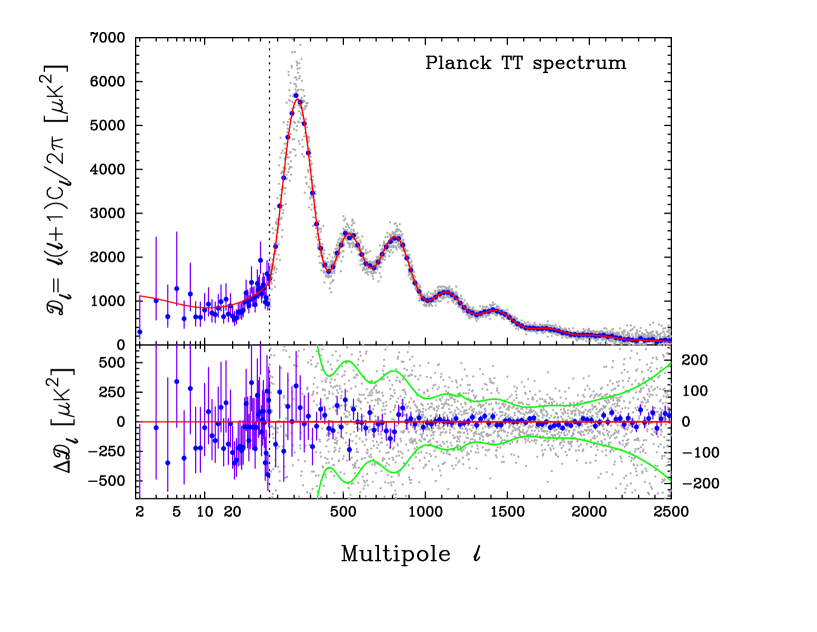
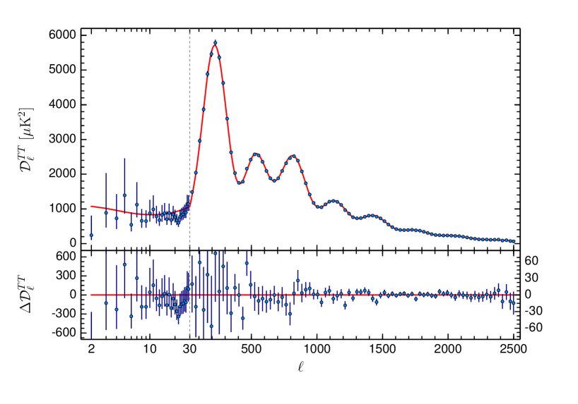
The Planck CMB data have been released for the first time in $2013$ Ade et al. (2013a) and, more recently, in $2015$, new measurements have been made public Planck:2015xua (1343079). Planck $2013$ has measured the CMB temperature anisotropies and the corresponding multipole moments $C_{\ell}^{{}_{\rm TT}}$ are represented in Fig. 4. Let us remind that these quantities are defined as follows. After foregrounds subtraction, the Planck measurements can be used to construct a map of the CMB temperature anisotropy, namely

$$\frac{\delta T}{T}({\bm{e}})=\sum_{\ell m}a_{\ell m}Y_{\ell m}({\bm{e}}),$$ (1.218)

where $Y_{\ell m}$ are the spherical harmonics and where the vector ${\bm{e}}$ specifies a direction in the sky. In practice, $\delta T/T$ can be expressed as

$$\frac{\delta T}{T}({\bm{e}})=\int\frac{{\rm d}{\bm{k}}}{(2\pi)^{3/2}}\left[F({\bm{k}})+G({\bm{k}})\frac{\partial}{\partial\eta_{0}}\right]{\rm e}^{id_{\rm A}{\bm{k}}\cdot{\bm{e}}/a(\eta_{\rm lss})}\,,$$ (1.219)

where $d_{\rm A}=a(\eta_{\rm lss})r_{0}+a(\eta_{\rm lss})\left(\eta_{0}-\eta_{\rm lss}\right)$ ($r_{0}$ being Earth’s radial coordinate and $\eta_{0}$ denoting the present time) is the angular distance to the surface of last scattering and the quantity ${\bm{k}}/a(\eta_{\rm lss})$ represents the physical wavenumber of the Fourier mode under consideration at the time of recombination. The quantities $F({\bm{k}})$ and $G({\bm{k}})$ encode the behavior of cosmological perturbations and are called “form factors” in Ref. Weinberg (2002). Already at this stage, we see that the configuration where the wavelengths of the perturbations become equal to the angular distance of the last scattering surface plays a preferred role. Then, the two-point correlation function in real space can be written as

$$\left\langle\frac{\delta T}{T}({\bm{e}}_{1})\frac{\delta T}{T}({\bm{e}}_{2})\right\rangle=\frac{1}{4\pi}\sum_{\ell=0}^{+\infty}(2\ell+1)C_{\ell}^{{}_{\rm TT}}P_{\ell}(\cos\theta),$$ (1.220)

where $\theta$ is the angle between the two vectors ${\bm{e}}_{1}$ and ${\bm{e}}_{2}$. This expression defines the multipole moments $C_{\ell}^{{}_{\rm TT}}$.

The big novelty of the Planck $2015$ data Planck:2015xua (1343079); Ade et al. (2015a) is that they not only lead to a more accurate measurements of the $C_{\ell}^{{}_{\rm TT}}$, see Fig. 5, but they also provide measurements of the $E$-mode CMB polarization. One can then define quantities similar to the $C_{\ell}^{{}_{\rm TT}}$ for the correlation between temperature and $E$-mode polarization fluctuations and for the $E$-mode power spectrum. The corresponding multipole moments $C_{\ell}^{{}_{\rm TE}}$ and $C_{\ell}^{{}_{\rm EE}}$ are represented in Figs. 6 and 7.

Figure 6: Multipole moments corresponding to the correlation between temperature and $E$-mode polarization anisotropies obtained from Planck $2015$. The red solid line corresponds to the best fit obtained with temperature measurements only. The lower panel shows the residual with respect to this best fit. Figure taken from Ref. Planck:2015xua (1343079).

Figure 7: Same as in Fig. 6 but for the $E$-mode power spectrum obtained from Planck $2015$. Figure taken from Ref. Planck:2015xua (1343079).

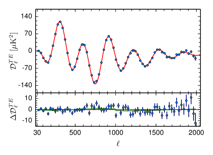
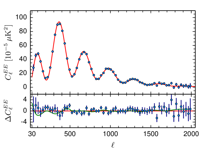
Before focusing on the consequences of these data for inflation, let us briefly discuss their implications for the standard model of Cosmology. It is important to understand that the constraints on the cosmological parameters can depend on the model analyzed and on the data used to perform the analysis. In $2013$, Planck used the temperature anisotropy measurement plus the WMAP polarization measurement on large scales ($\ell\leq 23$), the corresponding likelihood function being denoted PlanckTT+WP. In $2015$, at least five different likelihoods have been used: PlanckTT utilizes temperature data only and is an hybrid, meaning that the temperature likelihood is not the same for low multipoles ($\ell\leq 30$) and high multipoles; PlanckTT+lowP makes use of PlanckTT and low-$\ell$ polarization data; PlanckTE+lowP corresponds to the TE likelihood at $\ell\geq 30$ plus low-$\ell$ polarization data only; PlanckTT,TE,EE +lowP makes use of the TT, TE and EE likelihoods at $\ell\geq 30$ and of the temperature and polarization data at small scales. Depending on which likelihood is used, the constraints on cosmological parameters can slightly change.

The theoretical framework used to analyze the data is the flat [i.e. ${\cal K}=0$ in Eq. (1.1)] $\Lambda$CDM model. In order to specify it, we need to know the energy budget of the Universe, i.e. the photon energy density $\rho_{\gamma}$, the neutrino energy density $\rho_{\nu}$, the baryons energy density $\rho_{\rm b}$, the cold dark matter energy density $\rho_{\rm c}$ and the dark energy density $\rho_{\Lambda}$ (here assumed to be a cosmological constant). Then, in principle, on can calculate the behavior of the scale factor $a(t)$ since we know $\rho\equiv\sum_{i}\rho_{i}$ in the right hand side of the Friedmann equation (1.1). Of course we also need the Hubble rate today, $H_{0}$ or $h\equiv H_{0}/(100\,\mbox{km}\times\mbox{s}^{-1}\times\mbox{Mpc}^{-1})$ which is, therefore, another free parameter. We also need the power spectrum of scalar fluctuations assumed to be of the power-law form $P(k)\propto A_{{}_{\rm S}}k^{n_{{}_{\mathrm{S}}}-1}$ where $A_{{}_{\rm S}}$ is the amplitude of the fluctuations and $n_{\scriptscriptstyle{\mathrm{S}}}$ the spectral index. Here, gravitational waves are supposed to be absent, $r=0$. So, in this simple framework, the perturbations are characterized by two numbers. In the case of inflation, we need three parameters, the amplitude of scalar fluctuations and the two first slow-roll parameters. We notice (again!) that the parametrization used here is different from what we generically obtain from inflation where the power spectrum is not of the power-law form and where $r$ is necessarily non-vanishing (but can be very small). Finally, we need a parameter describing reionization and we take the optical depth $\tau$. The interpretation of this parameter is as follows. After recombination, the photons are supposed to propagate freely from the surface of last scattering to us. However, at the epoch of the formation of the first stars, estimated to be $z_{\rm re}\sim 10$, the Universe is ionized again. As a consequence, some of the CMB photons scatter off free electrons again. The probability to “avoid” this additional scattering is ${\rm e}^{-\tau}$ where

$$\tau\equiv\sigma_{{}_{\rm T}}\int_{t_{\rm re}}^{t_{\rm now}}n_{\rm e}{\rm d}t,$$ (1.221)

is the optical depth. In this expression, $\sigma_{{}_{\rm T}}$ is the Thomson cross-section and $n_{\rm e}$ is the number density of free electrons. When additional scattering occur, the direction of the photon change randomly and this washes out the CMB anisotropy on small angular scales, $\ell>\ell_{\rm re}$, namely $a_{\ell m}\rightarrow a_{\ell m}{\rm e}^{-\tau}$. For $\ell<\ell_{\rm re}$, the CMB anisotropies are not changed. The value of $\ell_{\rm re}$ clearly depends on $z_{\rm re}$. The previous considerations imply that, on small scales, the amplitude of the fluctuations becomes $A_{{}_{\rm S}}{\rm e}^{-2\tau}$ and there is therefore a partial degeneracy between $A_{{}_{\rm S}}$ and $\tau$.

In the Planck papers, one of the free parameters is in fact taken to be $\theta_{{}_{\rm MC}}$, where the subscript “MC” reminds that this quantity is used in COSMOMC. By definition, it is equal to be $\theta_{{}_{\rm MC}}\equiv 100(r_{{}_{\rm S}}/d_{\rm A})|_{\rm approx}$. Here, $r_{{}_{\rm S}}$ is the sound horizon at last scattering, namely

$$r_{{}_{\rm S}}=\int_{0}^{\eta_{\rm lss}}c_{{}_{\rm S}}{\rm d}\eta,$$ (1.222)

where $c_{{}_{\rm S}}$ is the sound speed of the baryon-photon fluid, i.e.

$$c_{{}_{\rm S}}^{2}=\frac{\delta p_{{\rm b}-\gamma}}{\delta\rho_{{\rm b}-\gamma}}=\frac{\delta p_{\gamma}}{\delta\rho_{\rm b}+\delta\rho_{\gamma}}=\frac{1}{3}\frac{4\rho_{\gamma}}{4\rho_{\gamma}+3\rho_{\rm b}}=\frac{1}{3}\frac{1}{1+R},$$ (1.223)

where $R=3\rho_{\rm b}/(4\rho_{\gamma})$. The quantity $d_{\rm A}$ is, as already mentioned, the angular distance to the last scattering surface and naturally appears in the expression of the multipole moments, see Eq. (1.219). Therefore, $r_{{}_{\rm S}}/d_{\rm A}$ is in fact the angular size of the sound horizon. $\theta_{{}_{\rm MC}}$ is defined approximately because its value is calculated at a redshift which is given by a fitting formula Hu and Sugiyama (1996)

$$z_{\rm lss}=1048\left[1+0.00124\left(\Omega_{\rm b}h^{2}\right)^{-0.738}\right]\left[1+g_{1}\left(\Omega_{\rm m}h^{2}\right)^{g_{2}}\right],$$ (1.224)

where the function $g_{1}$ and $g_{2}$ can be expressed as

$$g_{1} = 0.0783\left(\Omega_{\rm b}h^{2}\right)^{-0.238}\left[1+39.5\left(\Omega_{\rm m}h^{2}\right)^{0.763}\right]^{-1},$$ (1.225)

$$g_{2} = 0.560\left[1+21.1\left(\Omega_{\rm b}h^{2}\right)^{1.81}\right]^{-1}.$$ (1.226)

with $\Omega_{\rm m}=\Omega_{\rm b}+\Omega_{\rm c}$. In practice, instead of including $h$ in the list of free parameters, we consider $\theta_{{}_{\rm MC}}$.

We conclude that, a priori, we have a $9$ parameters: $h$ or $\theta_{{}_{\rm MC}}$, $\rho_{\gamma}$, $\rho_{\nu}$, $\rho_{\rm b}$, $\rho_{\rm c}$, $\rho_{\Lambda}$, $A_{{}_{\rm S}}$, $n_{\scriptscriptstyle{\mathrm{S}}}$ and $\tau$. However, the photon energy density is not a free parameter because it is given by $\pi^{2}T_{0}^{4}/15$ where $T_{0}=2.7255\pm 0.00006~{}\mbox{K}$ is the CMB temperature. In the same way, the neutrino energy density is fixed since $\rho_{\nu}=N_{\rm eff}(7/8)(4/11)^{4/3}\rho_{\gamma}$ with $N_{\rm eff}=3$. Moreover, the fact that the spatial sections are assumed to be flat means that, say $\rho_{\Lambda}$, can be deduced from the knowledge of the other parameters. Therefore, the “base” model used in the Planck articles is in fact a six-parameter scenario and it is sufficient to fit the CMB data.

Planck $2013$ (i.e. PlanckTT+WP using the terminology introduced before) found the following results ($68\%$ confidence limits) Ade et al. (2013a)

$$\Omega_{\rm b}h^{2} = 0.022032\pm 0.00028,\quad\Omega_{\rm c}h^{2}=0.1199\pm 0.0027,$$ (1.227)

$$100\theta_{{}_{\rm MC}} = 1.04131\pm 0.00063,\quad\tau=0.089^{+0.012}_{-0.014},$$ (1.228)

$$n_{\scriptscriptstyle{\mathrm{S}}} = 0.9603\pm 0.0073,\quad\ln\left(10^{10}A_{{}_{\rm S}}\right)=3.089^{+0.024}_{-0.027}.$$ (1.229)

On the other hand, Planck $2015$ with PlanckTT, TE, EE+lowP (as already mentioned, using the other likelihoods described before would lead to slightly different numbers) gives Planck:2015xua (1343079)

$$\Omega_{\rm b}h^{2} = 0.02225\pm 0.00016,\quad\Omega_{\rm c}h^{2}=0.1198\pm 0.0015,$$ (1.230)

$$100\theta_{{}_{\rm MC}} = 1.04077\pm 0.00032,\quad\tau=0.079\pm 0.017,$$ (1.231)

$$n_{\scriptscriptstyle{\mathrm{S}}} = 0.9645\pm 0.0049,\quad\ln\left(10^{10}A_{{}_{\rm S}}\right)=3.094\pm 0.0049.$$ (1.232)

The consistency between Planck $2013$ and Planck $2015$ is evidently very good.

More involved data analysis can be carried out by opening the parameter space (for instance by considering gravitational waves, a running for the scalar power spectrum, a time-dependent dark energy equation of state etc …) and/or adding more data sets. In the following, we will describe the corresponding results for the observables that are especially relevant for inflation.

V.1 Spatial Curvature

As discussed in Sec. III.1, see Eq. (1.23), maybe the most important prediction of inflation is that our Universe should be spatially flat (although there are contrived inflationary models for which this is not true Linde and Mezhlumian (1995)). Therefore, one can follow the strategy described above and relax the assumption that the curvature of spacelike sections is flat. Then, the Planck $2013$ data plus the WMAP data on large scale polarization imply that Ade et al. (2013a, b)

$$\Omega_{\cal K}=-0.058^{+0.046}_{-0.026}.$$ (1.233)

If, in addition, Baryonic Acoustic Oscillations (BAO) data are included, one obtains $\Omega_{\cal K}=-0.004\pm 0.0036$.

The Planck $2015$ Planck:2015xua (1343079) results have confirmed and tightened this conclusion. Indeed, at $95\%$ confidence level, PlanckTT,TE,EE+lowP leads to $\Omega_{\cal K}=-0.040^{+0.038}_{-0.041}$. If lensing data and BAO are taken into account, one arrives at the impressive following result

$$\Omega_{\cal K}=0.000\pm 0.005.$$ (1.234)

Therefore, we live in a spatially flat Universe in agreement with one of the most basic prediction of inflation.

As already mentioned, when one relaxes the assumption that the Universe is spatially flat, this introduces a new parameter and, therefore, we are no longer in the framework of the six-parameters $\Lambda$CDM base model considered before. As a consequence, a priori, the constraints on the other parameters may change. This is in particular the case of the spectral index $n_{\scriptscriptstyle{\mathrm{S}}}$ and its significant deviation from the scale-invariant case which is very important for inflation. However, Ref. Ade et al. (2015a) has shown that in the framework where $\Omega_{\cal K}\neq 0$ and where tensor modes are present, the constraint on $n_{\scriptscriptstyle{\mathrm{S}}}$ becomes

$$n_{\scriptscriptstyle{\mathrm{S}}}=0.969\pm 0.005,$$ (1.235)

using PlanckTT,TE,EE+lowP. The conclusion that the scale invariant case is ruled out seems therefore robust. In fact, Ref. Ade et al. (2015a) has shown that this conclusion is valid for other type of extensions such as different relativistic degrees of freedom (the parameter $N_{\rm eff}$ defined above, running, dark energy equation of state etc …). This is of course crucial for inflation.

V.2 Isocurvature Perturbations

Let us now investigate the Planck constraints on isocurvature perturbations Ade et al. (2013a, b, 2015a). We have discussed before, in Sec. IV.4, two types of isocurvature perturbations. Firstly, there is the effective mode taking into account cold dark matter and baryons entropy fluctuations, see Eq. (1.182) denoted, as already mentioned, CDI in the Planck papers. Secondly, there is also the Neutrino Density Isocurvature (NDI) mode and the Neutrino Velocity Isocurvature (NVI) mode. Each mode is characterized by its power spectrum as in Eq. (1.215) and each cross term can also be described by the correlation spectrum as in Eq. (1.217). Therefore, the most general situation can be parametrized by the $4\times 4$ matrix $\mathcal{P}_{ab}(k)$ where $a=\zeta,S_{\rm CDI},S_{\rm NDI},S_{\rm NVI}$ with the convention that $\mathcal{P}_{\zeta\zeta}\equiv\mathcal{P}_{\zeta}$ and similar expressions for the diagonal terms. Of course, this matrix is symmetrical.

Figure 8: Posterior distributions for the quantities $\alpha_{ab}\left(\ell_{\rm min},\ell_{\rm max}\right)$ introduced in Eq. (1.237), inferred from the Planck $2013$ data. No statistically significant deviation from adiabaticity is found. Notice that ${\cal R}=-\zeta$ is used in this plot. Figure taken from Ref. Ade et al. (2013b).

Figure 9: Two-dimensional distributions for the quantities $\mathcal{P}_{ab}(k_{1,2})\equiv\mathcal{P}_{ab}^{(1,2)}$ inferred from the Planck $2013$ data for $a=\mathcal{R}$, CDI (red), NDI (blue) and NVI (green). Again, amplitude of isocurvature spectra and correlation spectra are all consistent with adiabaticity. In these plots, notice that $\mathcal{P}_{ab}$ has indices $a=\mathcal{R}$, ${\cal I}$ with ${\cal I}\equiv\mbox{CDI},\mbox{NDI},\mbox{NVI}$. Figure taken from Ref. Ade et al. (2013b).

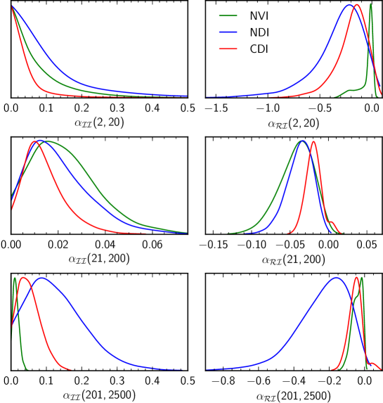
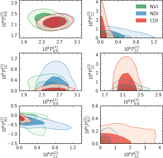
Usually, only a $2\times 2$ matrix is analyzed and a power law is assumed for each of the power spectra with independent spectral index. But this is not the route followed by the Planck team. Instead, they have assumed the following phenomenological form for $\mathcal{P}_{ab}(k)$

$$\mathcal{P}_{ab}(k)=\exp\left[\left(\frac{\ln k-\ln k_{2}}{\ln k_{1}-\ln k_{2}}\right)\ln\mathcal{P}_{ab}(k_{1})+\left(\frac{\ln k-\ln k_{1}}{\ln k_{2}-\ln k_{2}}\right)\ln\mathcal{P}_{ab}(k_{2})\right],$$ (1.236)

where the two scales $k_{1}$ and $k_{2}$ are chosen to be $k_{1}=2\times 10^{-3}\mbox{Mpc}^{-1}$ and $k_{2}=0.1\mbox{Mpc}^{-1}$ so that the entire Planck window is spanned. The positive definiteness of the matrix requires $\left(\mathcal{P}_{ab}\right)^{2}\leq\mathcal{P}_{aa}\mathcal{P}_{bb}$.

Then, the following quantities are defined

$$\alpha_{ab}\left(\ell_{\rm min},\ell_{\rm max}\right)=\frac{\left(\Delta T\right)^{2}_{ab}\left(\ell_{\rm min},\ell_{\rm max}\right)}{\left(\Delta T\right)^{2}_{\rm tot}\left(\ell_{\rm min},\ell_{\rm max}\right)},$$ (1.237)

where

$$\left(\Delta T\right)^{2}_{ab}\left(\ell_{\rm min},\ell_{\rm max}\right)=\sum_{\ell=\ell_{\rm min}}^{\ell=\ell_{\rm max}}\left(2\ell+1\right)C_{ab,\ell}^{\rm TT}.$$ (1.238)

In this expression, the quantity $C_{ab,\ell}^{\rm TT}$ represents the multipole moments calculated with the primordial spectrum taken to be $\mathcal{P}_{ab}$. $\left(\Delta T\right)^{2}_{\rm tot}$ is just the sum of all contributions. So, in the standard situation, there is just one contribution and the multipole moments are computed with $\mathcal{P}_{\zeta\zeta}=\mathcal{P}_{\zeta}$. If one has $\alpha_{\zeta\zeta}=1$, this means that the perturbations are fully adiabatic.

In Figs. 8 and 9, we have respectively represented the one-dimensional posterior distribution of $\alpha_{ab}\left(\ell_{\rm min},\ell_{\rm max}\right)$ and the two-dimensional distribution for the power spectra $\mathcal{P}_{ab}(k_{1,2})$ for the three modes, CDI, NDI and NVI obtained from Planck $2013$. The conclusion is clear: there is no statistically significant deviation from pure adiabaticity.

Figure 10: Two-dimensional distributions for the quantities $\mathcal{P}_{ab}(k_{1,2})\equiv\mathcal{P}_{ab}^{(1,2)}$ inferred from the Planck $2015$ for different choices of likelihoods indicated by different colors (gray, blue and red). This plot should be compared to Fig. 9. The six upper plots correspond to a situation where we have a mixture of adiabatic (denoted ADI) and CDI modes, the six middle plots to a situation where we have ADI and NDI and the bottom six plots to a case where one has ADI and NVI. Figure taken from Ref. Ade et al. (2015a).

Figure 11: Posterior distributions for the quantities $\alpha_{ab}\left(\ell_{\rm min},\ell_{\rm max}\right)$ introduced in Eq. (1.237), inferred from the Planck $2015$ data. This plot should be compared to Fig. 8. Figure taken from Ref. Ade et al. (2015a).

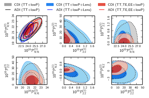
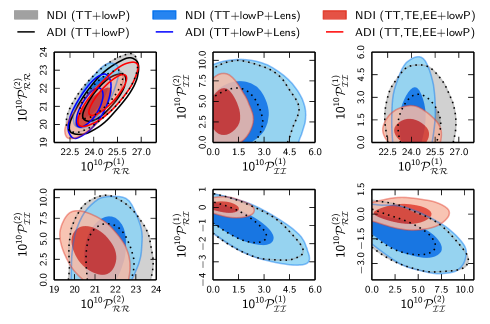
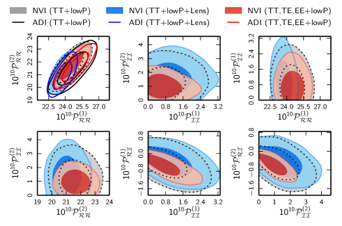
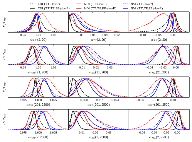
In Ref. Ade et al. (2015a), the constraints on isocurvature modes implied by the Planck $2015$ data have been derived. This work is particularly interesting since one expects the polarization data to have a good constraining power on the amplitude of the isocurvature modes. In this analysis, uniform priors for $\mathcal{P}_{\zeta\zeta}(k_{1})$ and $\mathcal{P}_{\zeta\zeta}(k_{2})$ are assumed in the range $\left[10^{-9},10^{-8}\right]$. For the power spectrum of the isocurvature power spectra, the same choice is made in the range $\left[0,10^{-8}\right]$. Finally, the adiabatic-isocurvature correlation function at $k=k_{1}$ is taken in the range $\left[-10^{-8},10^{8}\right]$. The same quantity, but at $k=k_{2}$, is fixed through an assumption about the correlation spectrum, see Eq. (1.217). Ref. Ade et al. (2015a) restricts itself to scale independent correlation spectrum,

$$\cos\Delta_{ab}=\frac{\mathcal{P}_{ab}}{\sqrt{\mathcal{P}_{aa}\mathcal{P}_{bb}}}$$ (1.239)

in the range $\left[-1,1\right]$. Writing the above equation at $k=k_{1}$ and $k=k_{2}$ and requiring that the value be the same (since the correlation spectrum is scale-independent) allows us to derive the parameter $\mathcal{P}_{ab}(k_{2})$.

The constraints on $\mathcal{P}_{ab}(k_{1})$ and $\mathcal{P}_{ab}(k_{2})$ obtained from Planck $2015$ are represented in Fig. 10. The constraints on the quantities $\alpha_{ab}(\ell_{\rm min},\ell_{\rm max})$ are displayed in Fig. 11. The conclusions obtained from Planck $2013$ are confirmed and even tightened. No isocurvature mode is detected and the primordial fluctuations are fully compatible with exact adiabaticity. This has of course very important implications for inflation. As explained before, this is a non trivial test for single-field slow-roll models. The Planck $2013$ data were compatible with this simple class of models and did not require to introduce additional fields. The results of Planck $2015$ do not modify this claim. As we are going to see in the next section, this is also the conclusion reached by the Planck measurements of Non-Gaussianities.

V.3 Non-Gaussianties

Let us now turn to the constraints on primordial Non-Gaussianity, see Ref. Ade et al. (2013c). Before discussing what was measured by the Planck satellite, it is interesting to review how the results are sometimes presented in the literature Komatsu (2010). In order to visualize the bispectrum, it is convenient to plot the quantity ${\cal B}_{{\mathcal{R}}}(k_{1},k_{2},k_{3})(k_{1}k_{2}k_{3})^{2}$ in terms of the ratios $x\equiv k_{3}/k_{1}$ and $y\equiv k_{2}/k_{1}$ with the conditions that ${\bm{k}}_{1}+{\bm{k}}_{2}+{\bm{k}}_{3}=0$ and $k_{1}\geq k_{2}\geq k_{3}$. This immediately implies that $0\leq x\leq 1$ and $0\leq y\leq 1$ and, therefore, the visualization can be restricted to this square, see Fig. 12. The fact that $k_{2}\geq k_{3}$ means that $y>x$ and, as a consequence, the red hatched region is in fact forbidden. Then, since the three vectors ${\bm{k}}_{1}$, ${\bm{k}}_{2}$ and ${\bm{k}}_{3}$ form a triangle, every edge length is smaller than the sum of the length of the two other edges. This means that $y>1-x$ and the green hatched region is also forbidden. The conditions $k_{2}<k_{1}+k_{3}$ (namely $y<1+x$) and $k_{3}<k_{1}+k_{2}$ (namely $y>x-1$) lead to new constraints but outside the square $[0,1]\times[0,1]$ and, therefore, are not interesting for us. The previous considerations show that it is sufficient to plot ${\cal B}_{{\mathcal{R}}}(k_{1},k_{2},k_{3})(k_{1}k_{2}k_{3})^{2}$ in the white, non hatched, region in Fig. 12 in order to have a complete representation of the bispectrum.

It is common practice to single out particular configurations. The squeezed triangle corresponds to $k_{1}\sim k_{2}\gg k_{3}$ which means $x\sim 0$ and $y\sim 1$. The equilateral configuration is given by $k_{1}\sim k_{2}\sim k_{3}$ or $x\sim y\sim 1$. The folded case is defined by $k_{1}\simeq 2k_{2}\simeq 2k_{3}$ or $x\sim y\sim 1/2$. These three configurations correspond to three vertices of the white triangle in Fig. 12. Another configuration is the elongated one for which $k_{1}\sim k_{2}+k_{3}$ or $x+y\sim 1$ and is therefore represented by a line in Fig. 12. The same is true for the isosceles triangle $k_{1}>k_{2}\sim k_{3}$ or $x\sim y$.

Figure 12: Visualization of the bispectrum shape. From the fact that the three vectors ${\bm{k}}_{1}$, ${\bm{k}}_{2}$ and ${\bm{k}}_{3}$ form a triangle, it is possible to faithfully represent the bispectrum in the white triangle. Then, different configurations correspond to vertices or edges of that triangle.

Figure 13: Bispectrum for different shape configuration: local (top left panel), equilateral (top right panel), orthogonal (bottom left panel). The bottom right panel represents the slow-roll prediction computed for a model where $V=m^{2}\phi^{2}/2$. Notice that the absolute normalization in these figures is irrelevant.

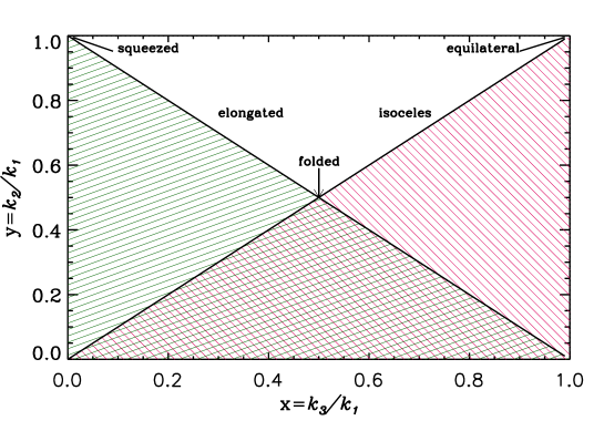
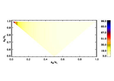
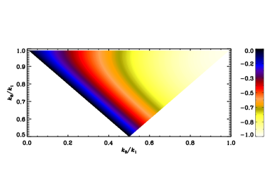
Let us now study how the local bispectrum looks like in this representation. From Eq. (1.135), one can write

$${\cal B}_{{\mathcal{R}}}(k_{1},k_{2},k_{3}) = -\frac{6f_{{}_{\mathrm{NL}}}^{\mathrm{loc}}}{5}(2\pi^{2})^{2}\frac{A_{{}_{\rm S}}^{2}}{k_{1}^{6}}\frac{1}{x^{3}y^{3}}(1+y^{3}+x^{3}).$$ (1.240)

where $\mathcal{P}(k)=A_{{}_{\rm S}}(k/k_{*})^{n_{\scriptscriptstyle{\mathrm{S}}}-1}$ and, for simplicity, we have taken $n_{\scriptscriptstyle{\mathrm{S}}}=1$ [strictly speaking, one should consider the power spectrum of Eq. (1.75) but, in fact, this does not change significantly the result of this calculation]. It follows, since ${\cal B}_{{\mathcal{R}}}(k_{1},k_{2},k_{3})(k_{1}k_{2}k_{3})^{2}=k_{1}^{6}y^{2}x^{2}{\cal B}_{{\mathcal{R}}}$ that

$${\cal B}_{{\mathcal{R}}}(k_{1},k_{2},k_{3})(k_{1}k_{2}k_{3})^{2}=-\frac{6f_{{}_{\mathrm{NL}}}^{\mathrm{loc}}A_{{}_{\rm S}}^{2}}{10}(2\pi^{2})^{2}\frac{1}{xy}(1+y^{3}+x^{3}).$$ (1.241)

In Fig. 13 (top left panel) we have represented this function (without the overall factor in the above expression). As it is clear from the plot (and also from the analytical expression), the local shape peaks at the squeezed triangle. The local shape has been constrained by the Planck 2013 data and one obtains Ade et al. (2013c) $f_{{}_{\mathrm{NL}}}^{\mathrm{loc}}=2.7\pm 5.8$ at $68\%{\rm CL}$. The Planck $2015$ data Ade et al. (2015b) with temperature only implies $f_{{}_{\mathrm{NL}}}^{\mathrm{loc}}=2.5\pm 5.7$ and including polarization data, one arrives at

$$f_{{}_{\mathrm{NL}}}^{\mathrm{loc}}=0.8\pm 5,$$ (1.242)

thus tightening the conclusion that the perturbations are Gaussian.

Another shape that was studied by the Planck team is the equilateral one. It is defined by

$${\cal B}_{{\mathcal{R}}}(k_{1},k_{2},k_{3}) = \frac{18}{5}f_{{}_{\mathrm{NL}}}^{\mathrm{eq}}(2\pi^{2})^{2}A_{{}_{\rm S}}^{2}\Biggl{[}\frac{1}{k_{1}^{3}k_{2}^{3}}+\frac{1}{k_{2}^{3}k_{3}^{3}}+\frac{1}{k_{1}^{3}k_{3}^{3}}+\frac{2}{(k_{1}k_{2}k_{3})^{2}}-\frac{1}{k_{1}k_{2}^{2}k_{3}^{3}}$$ (1.243)

$$-\frac{1}{k_{1}k_{3}^{2}k_{2}^{3}}-\frac{1}{k_{2}k_{1}^{2}k_{3}^{3}}-\frac{1}{k_{2}k_{3}^{2}k_{1}^{3}}-\frac{1}{k_{3}k_{1}^{2}k_{2}^{3}}-\frac{1}{k_{3}k_{2}^{2}k_{1}^{3}}\Biggr{]},$$

where, again, one has taken $n_{\scriptscriptstyle{\mathrm{S}}}=1$ for simplicity. One can re-express the bispectrum in terms of our variables $x$ and $y$ and then multiply by $(k_{1}k_{2}k_{3})^{2}$. This gives

$${\cal B}_{{\mathcal{R}}}(k_{1},k_{2},k_{3})(k_{1}k_{2}k_{3})^{2} = \frac{18}{5}f_{{}_{\mathrm{NL}}}^{\mathrm{eq}}(2\pi^{2})^{2}A_{{}_{\rm S}}^{2}\frac{1}{xy}\bigl{(}x^{3}+1+y^{3}+2xy-y-x-y^{2}$$ (1.244)

$$-y^{2}x-x^{2}-x^{2}y\bigr{)}.$$

The corresponding bispectrum has been represented in Fig. 13 (top right panel). The coefficient $f_{{}_{\mathrm{NL}}}^{\mathrm{eq}}$ has been constrained by Planck 2013 which finds Ade et al. (2013c) $f_{{}_{\mathrm{NL}}}^{\mathrm{eq}}=-42\pm 75$, a value compatible with zero. With the Planck $2015$ data Ade et al. (2015b) (temperature only), one obtains that $f_{{}_{\mathrm{NL}}}^{\mathrm{eq}}=-16\pm 70$ and, including polarization,

$$f_{{}_{\mathrm{NL}}}^{\mathrm{eq}}=-4\pm 43.$$ (1.245)

Finally, the last shape studied by Planck is the orthogonal one for which the bispectrum can be expressed as

$${\cal B}_{{\mathcal{R}}}(k_{1},k_{2},k_{3}) = \frac{18}{5}f_{{}_{\mathrm{NL}}}^{\mathrm{ortho}}(2\pi^{2})^{2}A_{{}_{\rm S}}^{2}\Biggl{[}\frac{3}{k_{1}^{3}k_{2}^{3}}+\frac{3}{k_{2}^{3}k_{3}^{3}}+\frac{3}{k_{1}^{3}k_{3}^{3}}+\frac{8}{(k_{1}k_{2}k_{3})^{2}}-\frac{3}{k_{1}k_{2}^{2}k_{3}^{3}}$$ (1.246)

$$-\frac{3}{k_{1}k_{3}^{2}k_{2}^{3}}-\frac{3}{k_{2}k_{1}^{2}k_{3}^{3}}-\frac{3}{k_{2}k_{3}^{2}k_{1}^{3}}-\frac{3}{k_{3}k_{1}^{2}k_{2}^{3}}-\frac{3}{k_{3}k_{2}^{2}k_{1}^{3}}\Biggr{]},$$

which leads to

$${\cal B}_{{\mathcal{R}}}(k_{1},k_{2},k_{3})(k_{1}k_{2}k_{3})^{2} = \frac{18}{5}f_{{}_{\mathrm{NL}}}^{\mathrm{ortho}}(2\pi^{2})^{2}A_{{}_{\rm S}}^{2}\frac{1}{xy}\bigl{(}3x^{3}+3+3y^{3}+8xy-3y-3x-3y^{2}$$ (1.247)

$$-3y^{2}x-3x^{2}-3x^{2}y\bigr{)},$$

and is plotted in Fig. 13 (bottom left panel). The coefficient $f_{{}_{\mathrm{NL}}}^{\mathrm{ortho}}$ has been measured by Planck 2013 and the result reads Ade et al. (2013c): $f_{{}_{\mathrm{NL}}}^{\mathrm{ortho}}=-25\pm 39$. This conclusion is confirmed by the Planck $2015$ measurements Ade et al. (2015b), namely $f_{{}_{\mathrm{NL}}}^{\mathrm{ortho}}=-34\pm 33$ (temperature only). If polarization data are included, then one finds

$$f_{{}_{\mathrm{NL}}}^{\mathrm{ortho}}=-26\pm 21.$$ (1.248)

Once again, the measured value is compatible with Gaussian primordial fluctuations.

It is also also interesting to represent explicitly the slow-roll result using the same visualization tools. This bispectrum was derived in Eq. (1.141). Expressed in terms of $x$ and $y$, each term ${\cal F}^{(i)}$ reads

$${\cal F}^{(1)} = \frac{H^{4}}{16M_{\scriptscriptstyle{\mathrm{Pl}}}^{4}\epsilon_{1}}k_{1}^{3}\Biggl{[}\left(1+\frac{1}{1+x+y}\right)\frac{x^{2}y^{2}}{1+x+y}+\left(1+\frac{y}{1+x+y}\right)\frac{x^{2}}{1+x+y}$$ (1.249)

$$+\left(1+\frac{x}{1+x+y}\right)\frac{y^{2}}{1+x+y}\Biggr{]},$$

$${\cal F}^{(2)} = \frac{H^{4}}{16M_{\scriptscriptstyle{\mathrm{Pl}}}^{4}\epsilon_{1}}\times-\frac{k_{1}^{3}}{2}(1+y^{2}+x^{2})\Biggl{[}-(1+x+y)+\frac{y+x+xy}{1+x+y}$$ (1.250)

$$+\frac{xy}{(1+x+y)^{2}}\Biggr{]}$$

$${\cal F}^{(3)} = -\frac{H^{4}}{16M_{\scriptscriptstyle{\mathrm{Pl}}}^{4}\epsilon_{1}}k_{1}^{3}\Biggl{[}\frac{1}{2}(-1+x^{2}-y^{2})\frac{x^{2}}{1+x+y}\Biggl{(}2+\frac{1+y}{1+x+y}\Biggr{)}$$ (1.251)

$$+\frac{1}{2}(-1-x^{2}+y^{2})\frac{y^{2}}{1+x+y}\Biggl{(}2+\frac{1+x}{1+x+y}\Biggr{)}$$

$$+\frac{1}{2}(-1-x^{2}-y^{2})\frac{1}{1+x+y}\Biggl{(}2+\frac{x+y}{1+x+y}\Biggr{)}\Biggr{]}$$

$${\cal F}^{(7)} = \frac{H^{4}}{16M_{\scriptscriptstyle{\mathrm{Pl}}}^{4}\epsilon_{1}}k_{1}^{3}\frac{\epsilon_{2}}{2\epsilon_{1}}(1+x^{3}+y^{3}).$$ (1.252)

If we write ${\cal F}^{(i)}\equiv H^{4}/(16M_{\scriptscriptstyle{\mathrm{Pl}}}^{4}\epsilon_{1})k_{1}^{3}f^{(i)}=(2\pi)^{2}\epsilon_{1}A_{{}_{\rm S}}^{2}k_{1}^{3}f^{(i)}$, then we see from the above equations (1.249), (1.250), (1.251) and (1.252) that the functions $f^{(i)}$ only depend on $x$ and $y$. In particular, this definition factors out the term $k_{1}^{3}$. As a consequence, using Eq. (1.141), the quantity ${\cal B}_{{\mathcal{R}}}^{\rm sr}(k_{1},k_{2},k_{3})(k_{1}k_{2}k_{3})^{2}$ can be written as Hazra et al. (2013)

$${\cal B}_{{\mathcal{R}}}^{\rm sr}(k_{1},k_{2},k_{3})(k_{1}k_{2}k_{3})^{2}=\left(2\pi^{2}\right)^{2}\epsilon_{1}\frac{A_{{}_{\rm S}}^{2}}{xy}\sum_{i=1,2,3,7}f^{(i)}(x,y).$$ (1.253)

This bispectrum is represented in Fig. 13 (bottom right panel). We notice that it is similar (up to a sign) to the equilateral shape (1.243).

Finally, Planck 2013 has also measured the four point correlation function for the local configuration. The corresponding constrain on the $\tau_{{}_{\rm NL}}$ reads Ade et al. (2013c)

$$\tau_{{}_{\rm NL}}<2800,$$ (1.254)

at $95\%$ confidence level, that is to say, a result compatible with Gaussianity. A recent analysis Feng et al. (2015) has confirmed this conclusion. Ref. Feng et al. (2015) has indeed found $\tau_{{}_{\rm NL}}=0.3\pm 0.9\times 10^{4}$ and $g_{{}_{\rm NL}}=-1.2\pm 2.8\times 10^{5}$. Finally, Planck $2015$ Ade et al. (2015b) obtained $g_{{}_{\rm NL}}=(-9.0\pm 7.7)\times 10^{4}$ at $68\%$ confidence level.

We conclude this section on Non-Gaussianity measurements as we concluded the section on isocurvature modes: the fact that we do not detect a signal beyond the vanilla situation is another non-trivial test for single-field slow-roll inflation with a minimal kinetic term. In the remaining part of this review, we therefore focus on this class of models and derive the corresponding implications that can inferred from the Planck data.

V.4 Slow-Roll Inflation

Figure 14: Two dimensional posterior distributions of the parameters $\epsilon_{1}$, $\epsilon_{2}$, $\epsilon_{3}$ and $P_{*}$ obtained from the Planck 2013 data. The pivot scale is chosen to be $k_{*}=0.05\mathrm{Mpc}^{-1}$ and the priors are taken to be as follows: a Jeffreys’ prior (i.e. a flat prior on the logarithm of the corresponding quantity) for $P_{*}$ such that $\ln(10^{10}P_{*})\in[2.7,4.2]$, a Jeffreys’ prior for $\epsilon_{1}$ such that $\log(\epsilon_{1})\in[-5,-0.7]$ (the choice of the upper bound ensures that $\epsilon_{1}<0.2$ and, therefore, that the slow-roll approximation is valid) and flat priors for $\epsilon_{2}$ and $\epsilon_{3}$ such that $\epsilon_{2}\in[-0.2,0.2]$ and $\epsilon_{3}\in[-0.2,0.2]$. Figure taken from Ref. Martin et al. (2014b).

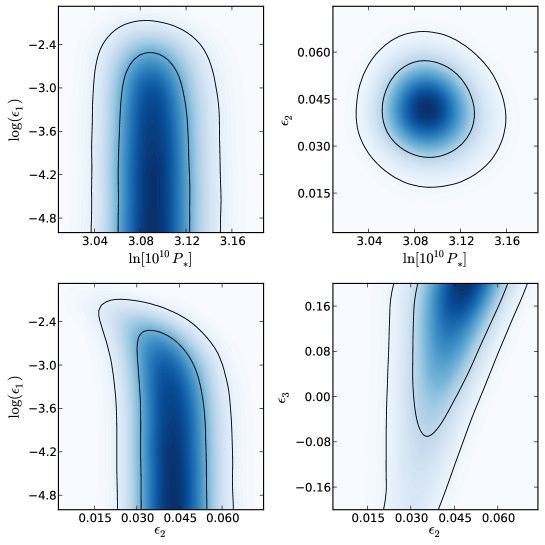
We have seen in Sec. IV.1 that the power spectra of scalar and tensor perturbations can be expressed in terms of the slow-roll parameters. Since the CMB measurements constrain the power spectra, they also constrain the slow-roll parameters Martin et al. (2014e). In Fig. 14, we show the two dimensional marginalized posterior distributions for the parameters $\epsilon_{1}$, $\epsilon_{2}$, $\epsilon_{3}$ and $P_{*}$, where this last quantity represents the overall normalization of the power spectrum obtained from the Planck 2013 data. We see that $P_{*}$ and $\epsilon_{2}$ are well constrained while there only exists an upper bound on $\epsilon_{1}$ and almost no constraints on $\epsilon_{3}$. Explicitly, one has $3.035\lesssim\ln\left(10^{10}P_{*}\right)\lesssim 3.15$, $\log\left(\epsilon_{1}\right)\lesssim-2.01$ and $0.023\lesssim\epsilon_{2}\lesssim 0.063$ at the two sigma level. Planck $2015$ Ade et al. (2015a) has also analyzed this question and found $\epsilon_{1}<0.0068$ and $\epsilon_{2}=0.029^{+0.008}_{-0.007}$ using PlanckTT+lowP and restricting the hierarchy at first order in slow-roll. When high-$\ell$ polarization data are included in the analysis, one finds $\epsilon_{1}<0.0066$ and $\epsilon_{2}=0.030^{+0.007}_{-0.006}$.

Let us now discuss the physical information on inflation that can be inferred from the above results. Firstly, from Eqs. (1.75) and (1.76), one has at next-to-leading order on slow-roll

$$P_{*}=\mathcal{P}_{\zeta 0}a_{0}=\frac{H_{*}^{2}}{8\pi^{2}\epsilon_{1*}M_{\scriptscriptstyle{\mathrm{Pl}}}^{2}}\left[1-2\left(C+1\right)\epsilon_{1}-C\epsilon_{2}\right],$$ (1.256)

from which we deduce that, at second order in slow-roll, the Hubble parameter during inflation can be expressed as Martin et al. (2014e)

$$\dfrac{H_{*}^{2}}{M_{{}_{\rm Pl}}^{2}} =8\pi^{2}\epsilon_{1}P_{*}\left[1+2(1+C)\epsilon_{1}+C\epsilon_{2}\right].$$ (1.257)

Since we know the posterior of $P_{*}$ and $\epsilon_{1}$, one can derive the corresponding one for $H_{*}$. The result is represented in Fig. 15, see the red dashed curves. Clearly, the fact that we only have an upper bound on $\epsilon_{1}$ implies that we also only have an upper bound on $H_{*}$. With the Jeffreys’ prior on $\epsilon_{1}$ (see the left panel in Fig. 15), one obtains $\ln\left(10^{5}\dfrac{H_{*}}{M_{{}_{\rm Pl}}}\right)\lesssim 1.6$, that is to say

$$H_{*}\lesssim 1.2\times 10^{14}\mathrm{GeV}.$$ (1.258)

One obtains a similar number if a flat prior on $\epsilon_{1}$ is assumed (see the right panel in Fig. 15). Those values can be expressed into gravitating energy scales through

$$\rho_{*}^{1/4}=3^{1/4}\sqrt{H_{*}M_{{}_{\rm Pl}}}\lesssim 2.2\times 10^{16}\mathrm{GeV},$$ (1.259)

where this value assumes a Jeffreys’ prior on $\epsilon_{1}$ (again, a similar result is obtained with a flat prior). If primordial gravity waves are detected, then this would fix the value of $r$ and, hence, the energy scale of inflation. This is illustrated in Fig. 15 where we have also plotted the posterior distribution of $H_{*}$ obtained when the BICEP2 results Ade et al. (2014a) are taken into account (assuming, for the sake of illustration, that they correspond to a detection of gravity waves).

Figure 15: Marginalized posterior distribution for the inflationary Hubble parameter at the time of pivot crossing with a Jeffreys’ prior (left panel) and a flat panel (right panel) on $\epsilon_{1}$ (left panel). The dashed red line represents the distribution obtained from the Planck 2013 data while the solid black line corresponds to the case where the Planck 2013 data are combined with the BICEP2 measurement (here, interpretated as a detection of gravity waves) and illustrates how a detection of primordial gravitational waves could allow us to determine the energy scale of inflation. Figure taken from Ref. Martin et al. (2014e).

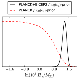
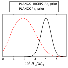
Secondly, let us now study what the constraints on the slow-roll parameters mean for the shape of the inflation potential Martin et al. (2014e). From Eq. (1.34), we see that this gives an upper bound on the first derivative of the inflation potential, namely

$$\left|V_{\phi}\right|\lesssim 0.14\frac{V}{M_{\scriptscriptstyle{\mathrm{Pl}}}}.$$ (1.260)

Using PlanckTT+lowP, the recent Planck $2015$ data Ade et al. (2015a) implies that $|V_{\phi}|\lesssim 0.116\left(V/M_{\scriptscriptstyle{\mathrm{Pl}}}\right)$. On the other hand, the second Hubble flow parameter gives information about the second derivative of the inflaton potential. From Eq. (1.35), one sees that

$$M_{\scriptscriptstyle{\mathrm{Pl}}}^{2}\frac{V_{\phi\phi}}{V}=2\epsilon_{1}-\frac{\epsilon_{2}}{2}.$$ (1.261)

From this expression, we also obtain bounds on the second derivative of the potential. Indeed, one has $M_{\scriptscriptstyle{\mathrm{Pl}}}^{2}V_{\phi\phi}/V>-\epsilon_{2{\rm sup}}$ and $M_{\scriptscriptstyle{\mathrm{Pl}}}^{2}V_{\phi\phi}/V<2\epsilon_{1{\rm sup}}-\epsilon_{2{\rm min}}/2$. Explicitly, one has

$$-0.03\lesssim M_{\scriptscriptstyle{\mathrm{Pl}}}^{2}\frac{V_{\phi\phi}}{V}\lesssim 0.008.$$ (1.262)

Planck $2015$ Ade et al. (2015a), using PlanckTT+lowP, finds the following value $M_{\scriptscriptstyle{\mathrm{Pl}}}^{2}V_{\phi\phi}/V=-0.01^{+0.005}_{-0.009}$ at $95\%$ confidence level.

Figure 16: Marginalized posterior distributions for the derived power law parameters $n_{\scriptscriptstyle{\mathrm{S}}}$, $r$, $n_{\scriptscriptstyle{\mathrm{T}}}$, $\alpha_{\scriptscriptstyle{\mathrm{S}}}$, $\alpha_{\scriptscriptstyle{\mathrm{T}}}$ and $\beta_{\scriptscriptstyle{\mathrm{T}}}$ obtained by importance sampling from the distributions of the second order slow-roll parameters. The dashed red line and the dotted green lines are the distributions obtained from Planck 2013. We have also represented the results obtained by combining Planck 2013 with BICEP2 (see the solid black line and the dotted dashed blue line). The most striking feature which would follow from a detection of gravity waves (here illustrated by including the BICEP2 results taken at face value) is of course that $r$, and therefore $n_{\scriptscriptstyle{\mathrm{T}}}$ using the slow-roll consistency relations (1.267), would now be measured. Figure taken from Ref. Martin et al. (2014e).

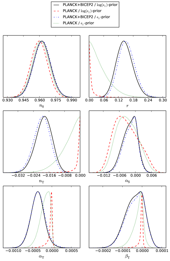
Thirdly, although the shape of the power spectrum is entirely characterized by Eq. (1.75), it is also interesting to derive constraints on the so-called power-law parameters Martin et al. (2014e). These parameters are in fact simple combinations of the Hubble flow parameters, as exemplified by Eqs. (1.86). We now investigate this question in more detail. In Eqs. (1.86), we gave the spectral indices at first order in slow-roll. At second order, they read

$$n_{\scriptscriptstyle{\mathrm{S}}} =1-(2\epsilon_{1}+\epsilon_{2})-2\epsilon_{1}^{2}-(3+2C)\epsilon_{1}\epsilon_{2}-C\epsilon_{2}\epsilon_{3},$$ (1.263)

$$n_{\scriptscriptstyle{\mathrm{T}}} =-2\epsilon_{1}-2\epsilon_{1}^{2}-2(1+C)\epsilon_{1}\epsilon_{2},$$

while the tensor-to-scalar ratio can be expressed as [see also Eq. (1.87)]

$$r=16\epsilon_{1}(1+C\epsilon_{2}).$$ (1.264)

One can also define the runnings for scalar and tensor and, in the slow-roll approximation, they are second-order quantities and their expressions read

$$\alpha_{\scriptscriptstyle{\mathrm{S}}}=-2\epsilon_{1}\epsilon_{2}-\epsilon_{2}\epsilon_{3},\qquad\alpha_{\scriptscriptstyle{\mathrm{T}}}=-2\epsilon_{1}\epsilon_{2},$$ (1.265)

Finally, let us mention that the running of the running for the tensor mode is also completely specified by the first three Hubble flow functions and is given by

$$\beta_{\scriptscriptstyle{\mathrm{T}}}=-2\epsilon_{1}\epsilon_{2}\left(\epsilon_{2}+\epsilon_{3}\right).$$ (1.266)

One sees that, in general, one has six independent quantities, namely $r$, $n_{\scriptscriptstyle{\mathrm{S}}}$, $n_{\scriptscriptstyle{\mathrm{T}}}$, $\alpha_{\scriptscriptstyle{\mathrm{S}}}$, $\alpha_{\scriptscriptstyle{\mathrm{T}}}$ and $\beta_{\scriptscriptstyle{\mathrm{T}}}$. However, the predictions of slow-roll inflation can be expressed in terms of three Hubble flow parameters (at least at this order), $\epsilon_{1}$, $\epsilon_{2}$ and $\epsilon_{3}$. This implies that all the parameters describing the tensor sector can, in fact, be expressed in terms of those characterizing the scalar sector. Explicitly, these so-called consistency relations can be expressed as

$$n_{\scriptscriptstyle{\mathrm{T}}} \simeq-\frac{r}{8},$$ (1.267)

$$\alpha_{\scriptscriptstyle{\mathrm{T}}} \simeq\frac{r}{8}\left[\frac{r}{8}+\left(n_{\scriptscriptstyle{\mathrm{S}}}-1\right)\right],$$

$$\beta_{\scriptscriptstyle{\mathrm{T}}} \simeq\frac{r}{8}\left[\frac{r}{8}+\left(n_{\scriptscriptstyle{\mathrm{S}}}-1\right)\right]\left(1-n_{\scriptscriptstyle{\mathrm{S}}}-\frac{r}{4}\right)+\frac{r}{8}\alpha_{\scriptscriptstyle{\mathrm{S}}}.$$

As before, since we know the posterior distributions of the slow-roll parameters for the Planck 2013 data, we can infer those of the power-law parameters. They are represented in Fig. 16, see the red dashed and dotted green lines. We see that the scalar spectral index $n_{\scriptscriptstyle{\mathrm{S}}}$ is very well constrained and is around $n_{\scriptscriptstyle{\mathrm{S}}}\simeq 0.96$ (the Planck $2013$ value, with WMAP large-angle polarization, reads $n_{\scriptscriptstyle{\mathrm{S}}}=0.9603\pm 0.0073$). On the other hand, we only have an upper bound on the tensor-to-scalar ratio which is of course expected since $r\propto\epsilon_{1}$. At two sigmas, one obtains $\log(r)\lesssim-0.88$ which gives

$$r\lesssim 0.13.$$ (1.268)

Notice that this result is obtained assuming a Jeffeys’ prior on $\epsilon_{1}$. If, instead, a flat prior is chosen, one has $\log(r)\lesssim-0.64$, leading to $r\lesssim 0.23$. This is because a flat prior has the tendency to favor large values of $r$ compared to what is obtained with a Jeffrey’s prior. In Fig. 16, we have also represented the results obtained by combining Planck 2013 and BICEP2 assuming that this last signal is due to primordial gravity waves. Of course, in that case $r$ is determined and, as a consequence, the tensor spectral index is also fixed. It is now known that the BICEP2 signal can be entirely explained by dust contamination Ade et al. (2014b) but, nevertheless, it is interesting to see what would be the implications for inflation of a detection of primordial gravity waves.

Recently, Planck $2015$ Ade et al. (2015a) has also put constraints on $r$. As usual, these constraints depend on the data sets used and on the assumptions made about the theoretical frameworks. Here we just quote two numbers. Using PlanckTT,TE,EE+lowP and considering that $r$ is the only extra parameter beyond the base $\Lambda$CDM model, one obtains

$$r_{0.002}<0.1,$$ (1.269)

at $95\%$ confidence limit. If instead PlanckTT+lowP+WP (we remind that WP means the polarization data on large scales measured by WMAP), this number becomes $r_{0.002}<0.09$. Here, the subscript “$0.002$” indicates that the pivot scale is taken to be $0.002\,\mbox{Mpc}^{-1}$.

Figure 17: $B$-mode CMB polarization multipole moments compared to the lensing signal (solid red curve). The black dots represent the values of $C_{\ell}^{\mathrm{BB}}$ obtained from the BICEP2/Keck array map. On recognizes the bump in the range $\ell\sim[50,120]$ that deviates from the lensing curve and that was interpreted as a detection of primordial gravity waves with $r\sim 0.16$ in Ref. Ade et al. (2014a). The blue dots correspond to the same multipole moments but after subtraction of the dust contribution, estimated from the cross-spectrum with the Planck $353$ GHz channel. Clearly, the new data are in good agreement with what is expected from lensing. Figure taken from Ref. BICEP2/Keck et al. (2015).

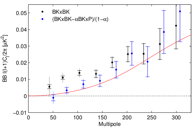
Very recently, a joint analysis by the BICEP2/Keck Array team and the Planck collaboration was released BICEP2/Keck et al. (2015). The results are presented in Fig. 17. In Ref. Ade et al. (2014a), BICEP2 announced the detection of primordial gravity waves at a level corresponding to a tensor-to-scalar ratio of $r\sim 0.16$. The reason for this claim can be seen in Fig. 17. In this plot, the red solid curve is the signal due to the weak lensing of $E$-mode that produces $B$-modes on small angular scales. This contribution is necessarily present in the standard model of Cosmology and its amplitude can be inferred unambiguously once we know the value of the cosmological parameters. The black dots represent the signal measured by BICEP2 and Keck Array. As is well visible, in the range $\ell\sim[50,120]$, there is an excess of power with respect to the red solid line and, hence, there must be another source of $B$-modes. BICEP2 interpreted this excess as a contribution coming from primordial gravity waves. However, there is another known source of contamination: dust. BICEP2 could not measure accurately the dust contribution because it operates at a single frequency only. The BICEP2 team therefore used theoretical models available at that time to remove the dust signal. On the other hand, Planck measures the CMB at different frequencies and, as a consequence, can estimate with good precision the dust contribution. It is therefore clear that a joint analysis between the two teams is the best way to use at the same time the good sensitivity of BICEP2/Keck Array and the good control of the dust signal of the Planck team. The result of this analysis are the blue dots in Fig. 17. We see that the bump has disappeared which means that the excess of power observed was probably entirely due to dust contamination and not to primordial gravity waves. The signal is now compatible with lensing. The new analysis suggests that the best value of $r$ is now $r\sim 0.05$ but with very low significance and $r\sim 0$ cannot be excluded. In other words, there is no longer a detection of primordial gravity waves. In addition, one obtains a new upper limit which is now $r<0.12$ (at $95\%$ confidence limit) instead of $r<0.11$ from the Planck $2013$ data. Notice that we obtained before $r<0.13$ from the Planck $2013$ data, see Eq. (1.268), and not $r<0.11$, but this is just due to some differences between our analysis and the Planck one (essentially, different priors).

In Ref. Martin et al. (2014e), it was demonstrated that the sets of inflationary models preferred by Planck alone and BICEP2 alone are almost disjoint, indicating a clear tension between the two data sets. Using a Bayesian measure of compatibility between BICEP2 and Planck, it was indeed shown that, for models favored by Planck $2013$ the two data sets tended to be incompatible, whereas there was a moderate evidence of compatibility for the BICEP2 preferred models. This means that the three assumptions (i) slow-roll inflation is the correct description of the early Universe (ii) Planck $2013$ data accurately measure CMB temperature anisotropies and (iii) BICEP2 measurement is due to primordial gravity waves are mutually exclusive. In other words, if one has the theoretical prejudice that slow-roll inflation did occur in the early Universe, then Ref. Martin et al. (2014e) already proved that the value $r\sim 0.16$ was likely to be overestimated. In some sense, the fact that dust contamination can explain the BICEP2 signal reinforces our trust in inflation!

Let us now turn to the scalar running $\alpha_{\scriptscriptstyle{\mathrm{S}}}$. At $95\%$ confidence level, one finds

$$-0.012\lesssim\alpha_{\scriptscriptstyle{\mathrm{S}}}\lesssim 0.006,$$ (1.270)

that is to say a value consistent with no running. Finally, one notices that the quantities $\alpha_{\scriptscriptstyle{\mathrm{T}}}$ and $\beta_{\scriptscriptstyle{\mathrm{T}}}$ are well-constrained. It is easy to understand why on the example of $\alpha_{\scriptscriptstyle{\mathrm{T}}}$. One has $\alpha_{\scriptscriptstyle{\mathrm{T}}}=(r/8)^{2}+(n_{\scriptscriptstyle{\mathrm{S}}}-1)(r/8)$, see Eq. (1.267). In this equation $n_{\scriptscriptstyle{\mathrm{S}}}-1$ is known, one can take $n_{\scriptscriptstyle{\mathrm{S}}}-1\simeq-0.04$ which means that $\alpha_{\scriptscriptstyle{\mathrm{T}}}\simeq(r/8)^{2}-0.04(r/8)$. This parabola has a minimum at $r/8\simeq 0.02$ which corresponds to $\alpha_{\scriptscriptstyle{\mathrm{T}}}\simeq-9\times 10^{-5}$. The maximum is for $r\simeq 0.13$ and gives $\alpha_{\scriptscriptstyle{\mathrm{T}}}\simeq-0.0004$. We therefore expect $-0.0004\lesssim\alpha_{\scriptscriptstyle{\mathrm{T}}}<-9\times 10^{-5}$ and which (roughly speaking) explains why the distribution of $\alpha_{\scriptscriptstyle{\mathrm{T}}}$ in Fig. 16 is peaked (see the red dashed line).

A last remark is in order at this point. Very often, as already pointed out, the power spectrum is parametrized as

$$\mathcal{P}_{\zeta}(k)=A_{{}_{\rm S}}\left(\frac{k}{k_{*}}\right)^{n_{\scriptscriptstyle{\mathrm{S}}}-1+\alpha_{\scriptscriptstyle{\mathrm{S}}}/2\ln(k/k_{*})+\cdots},$$ (1.271)

and a similar expression for the tensors. Clearly, this is not exactly what inflation predicts since not expanding $n_{\scriptscriptstyle{\mathrm{S}}}-1=-2\epsilon_{1}-\epsilon_{2}$ (if one works at first order in slow-roll) in the above formula means in fact keeping an infinite number of higher order corrections which is clearly inconsistent since $n_{\scriptscriptstyle{\mathrm{S}}}$ is determined at a fixed order. Of course, since $n_{\scriptscriptstyle{\mathrm{S}}}-1$ is small, for all practical purposes, this does not impact a lot the final results.

V.5 Model Comparison

Let us now turn to model comparison Martin et al. (2011, 2014a, 2014b, 2014e). We would like to determine the models of inflation that perform the best being given the current CMB data. From a statistical point of view, this question is subtle. Indeed, suppose we have two models: $\mathcal{M}_{1}$ characterized by one parameter $\theta_{11}$ and $\mathcal{M}_{2}$ characterized by two parameters $\theta_{21}$, $\theta_{22}$. What does it mean to claim that model $\mathcal{M}_{1}$ is better than model $\mathcal{M}_{2}$ (or the opposite)? Naively, one could compare the likelihoods of the two models for the values of the parameters leading to the best fits. But model $\mathcal{M}_{2}$ has one extra parameter and, therefore, one expects this model to automatically improve the fit. Therefore, in some sense, it would be “unfair” to claim that $\mathcal{M}_{2}$ is better than $\mathcal{M}_{1}$ since it is “more complicated”. Moreover, suppose that only for, say, $\theta_{21}\in\left[10^{-20},10^{-19}\right]$ does $\mathcal{M}_{2}$ lead to a good $\chi^{2}$ while, a priori, $\theta_{12}$ could vary, in say $[-1,1]$. Suppose, in addition, that this does not happen for $\mathcal{M}_{1}$, namely that for $\theta_{11}$ in its natural range of variation, the fit is always “reasonable”. How do we take into account this wasted parameter space for model $\mathcal{M}_{2}$ in our assessment of the respective performance of the two models?

In order to answer these questions, one recalls that if $\mathcal{L}_{2}(\theta_{21},\theta_{22})\equiv p(D|\theta_{21},\theta_{22},\mathcal{M}_{2})$ is the likelihood of model $\mathcal{M}_{2}$ ($D$ represents the data, here we have of course CMB data in mind), then the probability of the parameters $\theta_{21},\theta_{22},$ can be expressed as (the Bayes’ theorem) Trotta (2008)

$$p(\theta_{21},\theta_{22}|D,\mathcal{M}_{2})=\frac{1}{\mathcal{E}(D|\mathcal{M}_{2})}\mathcal{L}_{2}(\theta_{21},\theta_{22})\pi(\theta_{21}|\mathcal{M}_{2})\pi(\theta_{22}|\mathcal{M}_{2}),$$ (1.272)

where $\pi$ represents the prior distributions and $\mathcal{E}$ is a normalization factor which depends on the data and the model. We would like to calculate the probability $p(\mathcal{M}_{2}|D)$ of model $\mathcal{M}_{2}$ and, therefore, we expect a similar equation to hold, namely

$$p(\mathcal{M}_{2}|D)=\frac{1}{p(D)}p(D|\mathcal{M}_{2})\pi(\mathcal{M}_{2}),$$ (1.273)

where $p(D)$ is a normalization factor depending on the data only and $\pi$ encodes our a priori information about model $\mathcal{M}_{2}$. Clearly, Eqs. (1.272) and (1.273) have the same structure since they represent two applications of the Bayes’s theorem. To make progress we need to know $p(D|\mathcal{M}_{2})$. But this quantity is in fact easy to calculate since $\int p(\theta_{21},\theta_{22}|D,\mathcal{M}_{2}){\rm d}\theta_{21}{\rm d}\theta_{22}=1$, Eq. (1.272) leads to

$$\mathcal{E}(D|\mathcal{M}_{2}) = \int\mathcal{L}_{2}(\theta_{21},\theta_{22})\pi(\theta_{21}|\mathcal{M}_{2})\pi(\theta_{22}|\mathcal{M}_{2}){\rm d}\theta_{21}{\rm d}\theta_{22}$$ (1.274)

$$= \int p(D|\theta_{21},\theta_{22},\mathcal{M}_{2})\pi(\theta_{21}|\mathcal{M}_{2})\pi(\theta_{22}|\mathcal{M}_{2}){\rm d}\theta_{21}{\rm d}\theta_{22}$$

$$= p(D|\mathcal{M}_{2}).$$

Of course the previous considerations apply in general and the quantity $\mathcal{E}(D|\mathcal{M}_{i})$ is called the Bayesian evidence of the model $\mathcal{M}_{i}$ and its definition reads Trotta (2008)

$$p(D|\mathcal{M}_{i})\equiv\mathcal{E}\left(D|\mathcal{M}_{i}\right)=\int{\rm d}\theta_{ij}\mathcal{L}\left(\theta_{ij}\right)\pi\left(\theta_{ij}|\mathcal{M}_{i}\right).$$ (1.275)

The Bayesian evidence is often normalized to a reference model $\mathcal{M}_{\scriptscriptstyle{\mathrm{REF}}}$ and one defines $B^{i}_{{\scriptscriptstyle{\mathrm{REF}}}}\equiv\mathcal{E}(D|\mathcal{M}_{i})/\mathcal{E}(D|\mathcal{M}_{\scriptscriptstyle{\mathrm{REF}}})$. In that case, the posterior probability of the model $\mathcal{M}_{i}$ (for non-committal model priors) can be re-expressed as

$$p\left(\mathcal{M}_{i}|D\right)=\frac{B^{i}_{{\scriptscriptstyle{\mathrm{REF}}}}}{\sum_{j}B^{j}_{{\scriptscriptstyle{\mathrm{REF}}}}}\,.$$ (1.276)

In the following, we will give $B^{i}_{{\scriptscriptstyle{\mathrm{REF}}}}$ since this quantity is in one-to-one correspondence with the probability of the model $\mathcal{M}_{i}$. In particular, one sees that $p(\mathcal{M}_{i})>p(\mathcal{M}_{j})$, namely model $\mathcal{M}_{i}$ is better than $\mathcal{M}_{j}$ (or more probable), if $\mathcal{E}(\mathcal{M}_{i})>\mathcal{E}(\mathcal{M}_{j})$ or, equivalently, $B^{i}_{{\scriptscriptstyle{\mathrm{REF}}}}>B^{j}_{{\scriptscriptstyle{\mathrm{REF}}}}$.

Figure 18: $\ln B^{i}_{{\scriptscriptstyle{\mathrm{REF}}}}$ for the all single field slow-roll models with minimal kinetic terms. The reference model is taken to be the one where the priors are directly chosen on the Hubble flow parameters. Each model is represented by a bar, the length of which is directly proportional to $\ln B^{i}_{{\scriptscriptstyle{\mathrm{REF}}}}$ (the numerical value of $\ln B^{i}_{{\scriptscriptstyle{\mathrm{REF}}}}$ being indicated on the same line). A bar on the left means that $\ln B^{i}_{{\scriptscriptstyle{\mathrm{REF}}}}<0$ and a bar on the right that $\ln B^{i}_{{\scriptscriptstyle{\mathrm{REF}}}}>0$. The color code refers to the Schwarz-Cesaro Escalante classification Schwarz et al. (2001). The vertical dotted black line indicates the Jeffreys’ categories, see the text for more explanations. Figure taken from Ref. Martin et al. (2014b).

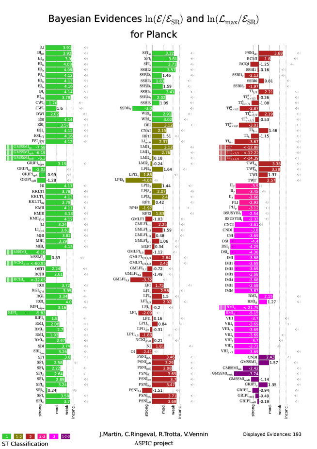
In order to see why computing the Bayesian evidence answers the questions asked before and can give a fair estimate of the performances of a model, let us consider the idealized following situation. Let us assume that the likelihood function of model $\mathcal{M}_{1}$ has width $\delta\theta_{11}$ and that the prior is flat and has width $\Delta\theta_{11}$. Since $\pi$ is normalized, we have $\pi(\theta_{11})=1/\Delta\theta_{11}$. We also assume that the likelihood is more informative than the prior, namely $\delta\theta_{11}<\Delta\theta_{11}$. Then, Eq. (1.275) is approximately given by

$$\mathcal{E}(D|\mathcal{M}_{1})\simeq\mathcal{L}_{1,{\rm max}}\frac{\delta\theta_{11}}{\Delta\theta_{11}}.$$ (1.277)

A similar calculation for $\mathcal{M}_{2}$ leads to

$$\mathcal{E}(D|\mathcal{M}_{2})\simeq\mathcal{L}_{2,{\rm max}}\frac{\delta\theta_{21}}{\Delta\theta_{21}}\frac{\delta\theta_{22}}{\Delta\theta_{22}}.$$ (1.278)

For simplicity, one can take the reference model to be model $\mathcal{M}_{1}$ and, of course, one has $B^{1}_{{\scriptscriptstyle{\mathrm{REF}}}}=1$. For $B^{2}_{{\scriptscriptstyle{\mathrm{REF}}}}$, one finds

$$B^{2}_{{\scriptscriptstyle{\mathrm{REF}}}}=\frac{\mathcal{L}_{2,{\rm max}}}{\mathcal{L}_{1,{\rm max}}}\frac{\Delta\theta_{11}}{\delta\theta_{11}}\frac{\delta\theta_{21}}{\Delta\theta_{21}}\frac{\delta\theta_{22}}{\Delta\theta_{22}}.$$ (1.279)

On this last equation, we see that deciding whether model $\mathcal{M}_{1}$ is better or worst than $\mathcal{M}_{2}$ does not reduce to the comparison of the likelihood function at the best fit, $\mathcal{L}_{2,{\rm max}}/\mathcal{L}_{1,{\rm max}}$ but that this ratio is corrected by a factor which describes how much parameter space has been wasted. So the best model is not the one which has the largest $\chi^{2}$ but the one which achieves the best compromise between quality of the fit and simplicity of the theoretical description.

As explained before, here, we focus on single-field slow-roll inflationary models (with minimal kinetic term) only. At this stage, the strategy is clear: one must evaluate the Bayesian evidence of each of these models in order to rank them according to their ability to fit the data. This first requires to identify all models of this type and this was recently done in Encyclopaedia Inflationaris, see Ref. Martin et al. (2014a). In this work, about $200$ models have been identified. A model corresponds to a specific choice of potential and of priors for its parameters. Two different models can have the same potential but different priors. Each model is denoted by an acronym according to the terminology introduced in Ref. Martin et al. (2014b) and, in the present article, we just make use of this convention. A detailed justification of the priors chosen can also be found in that reference. In Fig. 18, we have represented the Bayesian evidence of the different models (being given the Planck 2013 data) by an horizontal bar the length of which is proportional to $\ln B^{i}_{{\scriptscriptstyle{\mathrm{REF}}}}$, see also the caption of Fig. 18 and Refs. Martin et al. (2014a, b); Ringeval (2014); Martin et al. (2014e). In order to translate the numerical value of the evidence into strength of belief, we introduce the Jeffrey’s scale Trotta (2008). If $|\ln B^{i}_{{\scriptscriptstyle{\mathrm{REF}}}}|<1$, then the model is in the “inconclusive zone”, if $1<|\ln B^{i}_{{\scriptscriptstyle{\mathrm{REF}}}}|<2.5$, then it is in the “weak evidence zone”, if $2.5<|\ln B^{i}_{{\scriptscriptstyle{\mathrm{REF}}}}|<5$, then it is in the “moderate evidence zone” and, finally, if $|\ln B^{i}_{{\scriptscriptstyle{\mathrm{REF}}}}|<5$, it is in the “strong evidence zone”. If the reference model is taken to be the best model, then, by definition all $\ln B^{i}_{{\scriptscriptstyle{\mathrm{REF}}}}$ are negative. In that case, the best models are those in the inconclusive zone and those in the “strong evidence zone” can be considered as ruled out.

In Fig. 18, we see that the best Planck 2013 model is $\mathrm{KMIII}$ and that $52$ models end up being in the inconclusive zone, namely: $\mathrm{KMIII}$, $\mathrm{ESI}_{\sqrt{2}}$, $\mathrm{BI}_{6\mathrm{s}}$, $\mathrm{MHI}_{\mathrm{s}}$, $\mathrm{BI}_{\mathrm{s}}$, $\mathrm{ESI}$, $\mathrm{BI}_{5\mathrm{s}}$, $\mathrm{KKLTI}_{\mathrm{s}}$, $\mathrm{KMII}_{V>0}$, $\mathrm{BI}_{4\mathrm{s}}$, $\mathrm{ESI}_{\mathrm{o}}$, $\mathrm{ESI}_{\sqrt{2/3}}$, $\mathrm{KMII}$, $\mathrm{HI}$, $\mathrm{BI}_{3\mathrm{s}}$, $\mathrm{BI}_{2\mathrm{s}}$, $\mathrm{RGI}_{\mathrm{s}}$, $\mathrm{RGI}_{1/16}$, $\mathrm{BI}_{\mathrm{ph}}$, $\mathrm{AI}$, $\mathrm{BI}_{1\mathrm{s}}$, $\mathrm{MHI}$, $\mathrm{SFI}_{\mathrm{l}}$, $\mathrm{SFI}$, $\mathrm{KKLTI}_{\mathrm{stg}}$, $\mathrm{BI}_{\mathrm{stg}}$, $\mathrm{KKLTI}$, $\mathrm{SBI}$, $\mathrm{RGI}$, $\mathrm{SFI}_{\mathrm{s}}$, $\mathrm{PSNI}_{\mathrm{oA}}$, $\mathrm{SFI}_{4\mathrm{l}}$, $\mathrm{PSNI}_{\mathrm{ft2}}$, $\mathrm{PSNI}_{\mathrm{oB}}$, $\mathrm{PSNI}_{\mathrm{ft1}}$, $\mathrm{PSNI}_{\mathrm{oC}}$, $\mathrm{LI}_{\alpha>0}$, $\mathrm{SFI}_{4}$, $\mathrm{ESI}_{\mathrm{l}}$, $\mathrm{SSBI2}$, $\mathrm{PSNI}_{\mathrm{ft3}}$, $\mathrm{PSNI}_{\mathrm{epA}}$, $\mathrm{SSBI4}$, $\mathrm{TWI}_{\phi_{0}}$, $\mathrm{RGI}_{\mathrm{l}}$, $\mathrm{SFI}_{4\mathrm{s}}$, $\mathrm{MHI}_{\mathrm{l}}$, $\mathrm{PSNI}_{\mathrm{epB}}$, $\mathrm{TWI}_{\phi_{0}}^{\mathrm{r}}$, $\mathrm{SBI}_{\alpha_{\mathrm{min}}}$, $\mathrm{LI}$, $\mathrm{SFI}_{3\mathrm{l}}$. They represent $\sim 26\%$ of the models analyzed. We also find that $21\%$ of the models are in the “weak evidence zone”, $17\%$ in the “moderate evidence zone” and $34\%$ in the “strong evidence zone”. Planck 2013 is therefore able to rule out about one third of the inflationary models. Model comparison with Planck $2015$ data cannot yet be done since the scientific products are not delivered. However, given the consistency of these two data sets, we do not expect very different results.

We have seen before that the “winner” is $\mathrm{KMIII}$ which is a string inspired model with the following potential Conlon and Quevedo (2006)

$$V(\phi)=M^{4}\left[1-\alpha\left(\frac{\phi}{M_{\scriptscriptstyle{\mathrm{Pl}}}}\right)^{4/3}{\rm e}^{\beta(\phi/M_{\scriptscriptstyle{\mathrm{Pl}}})^{4/3}}\right],$$ (1.280)

where $\alpha$ and $\beta$ are two free parameters. Its heir apparent is $\mathrm{ESI}_{\sqrt{2}}$ the potential of which is given by Stewart (1995); Dvali and Tye (1999); Cicoli et al. (2009)

$$V(\phi)=M^{4}\left(1-{\rm e}^{-\sqrt{2}\phi/M_{\scriptscriptstyle{\mathrm{Pl}}}}\right).$$ (1.281)

The fourteenth on the list is the Starobinsky model Starobinsky (1980); Bezrukov and Shaposhnikov (2008), namely

$$V(\phi)=M^{4}\left(1-{\rm e}^{-\sqrt{2/3}\phi/M_{\scriptscriptstyle{\mathrm{Pl}}}}\right)^{2}.$$ (1.282)

Actually, all these models being in the “inconclusive zone”, the difference between their Bayesian evidence is not significant. This means that, for instance, one should view the Starobinsky model as as good as $\mathrm{KMIII}$. In fact, the main common point between all these scenarios is that they all possess a “plateau-like” potential, meaning that $V_{\phi}(\phi)\rightarrow 0$ as $\phi\rightarrow\infty$. We conclude that Planck 2013 has been able to constrain the shape of the inflationary potential, a truly remarkable achievement when one remembers that inflation can take place at $10^{15}\mathrm{GeV}$, and certainly something impossible to do in an accelerator!

We have seen before that, in order to explain the data, we do not need to consider models more complicated than single field slow-roll inflation with a minimal kinetic term. This does not mean that more complicated models are ruled out (in the frequentist point of view) in the sense that, with a carefully chosen set of parameters, they can lead to good fits. However, from the previous considerations, we see that those models must have a very “bad” Bayesian evidence. Computing the evidence of those more complicated models is certainly a difficult task (for instance, for models predicting a non negligible level of Non-Gaussianities, one would need to take into account the higher order correlation functions). But, in fact, we do not need to carry out such a calculation which, at this stage appears to be useless. Indeed we know in advance that they are much “worse” than single-field models because of their huge wasted parameter space Giannantonio and Komatsu (2015). It is sufficient to know that they all are in the “strong evidence zone” and, clearly, we are not much interested in knowing the ranking in this Jeffreys category since the models are ruled out (in the Bayesian sense) anyway.

Figure 19: Inflationary models in the space $\left(N_{\rm uc},\ln B^{i}_{{\scriptscriptstyle{\mathrm{REF}}}}\right)$. Each model is represented by a circle (the radius of which has no meaning) with its acronym, taken from Ref. Martin et al. (2014b), written inside. The four panels corresponds to successive zooms towards the best region (indicated by the dashed rectangles), the one with $0<N_{\rm uc}<1$, namely where all the parameters are constrained by the data and a large value of the evidence, namely the model achieves a good fit without wasting parameter space. Figures taken from Ref. Martin et al. (2014b).

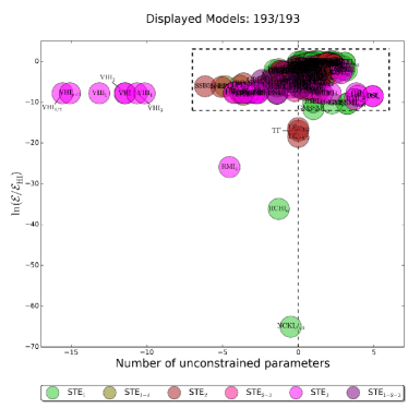
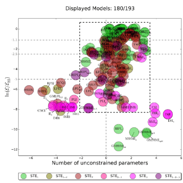
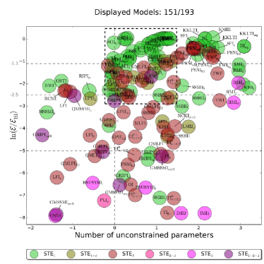
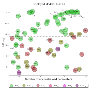
We have seen how the Bayesian evidence allows us to rank the various inflationary models. However, two models with a different number of parameters can have the same evidence if the extra parameters are not constrained by the data. This is certainly not a desirable property as the model with less parameters is clearly simpler and, therefore, should be favored. In order to break this degeneracy, we now introduce the Bayesian complexity Kunz et al. (2006). For a model $\mathcal{M}_{i}$, it is defined by Kunz et al. (2006)

$$C_{\rm b}^{i}=\left\langle-2\log{\cal L}\left(\theta_{ij}\right)\right\rangle+2\log{\cal L}\left(\theta_{ij}^{\rm ML}\right),$$ (1.283)

where $\langle\cdot\rangle$ means averaging over the posteriors and $\theta_{ij}^{\rm ML}$ represents the maximum likelihood estimate of the model’s parameters. One can easily show, see for instance Ref. Martin (2013), that the number of unconstrained parameters, given a data set, can be expressed as

$$N_{\rm uc}^{i}=N_{\rm param}^{i}-C_{\rm b}^{i},$$ (1.284)

where $N_{\rm param}^{i}$ represents the number of free parameters of model $\mathcal{M}_{i}$. We see that this gives us a new criterion to discriminate the various models since a model such that $0<N_{\rm uc}^{i}<1$ ought to be preferred. The Bayesian complexities (given the Planck 2013 data) of all the Encyclopaedia Inflationaris models have been computed in Ref. Martin et al. (2014b). In Fig. 19, we have represented these scenarios in the space $\left(N_{\rm uc},\ln B^{i}_{{\scriptscriptstyle{\mathrm{REF}}}}\right)$. It can be noticed that, among the models in the Planck 2013 inconclusive zone, those with a minimal number of unconstrained parameters are: $\mathrm{ESI}_{\sqrt{2}}$, $\mathrm{ESI}_{\sqrt{2/3}}$, $\mathrm{HI}$, $\mathrm{BI}_{2\mathrm{s}}$, $\mathrm{RGI}_{\mathrm{s}}$, $\mathrm{AI}$, $\mathrm{BI}_{1\mathrm{s}}$, $\mathrm{MHI}$, $\mathrm{RGI}$, $\mathrm{SFI}_{4\mathrm{l}}$, $\mathrm{LI}_{\alpha>0}$, $\mathrm{SFI}_{4}$, $\mathrm{ESI}_{\mathrm{l}}$, $\mathrm{RGI}_{\mathrm{l}}$, $\mathrm{MHI}_{\mathrm{l}}$, $\mathrm{SBI}_{\alpha_{\mathrm{min}}}$ and $\mathrm{SFI}_{3\mathrm{l}}$. The number of preferred models is now $17$, that is to say $\sim 9\%$ of the total number of models analyzed here. Of course, as already remarked, these models are all of the plateau shape. The distribution of models in the four Jeffreys categories versus the number of unconstrained parameters is summarized in Fig. 20.

Figure 20: Occurrences of inflationary models in the four Jeffreys categories for different values of the unconstrained number of parameters. Figure taken from Ref. Martin (2013).

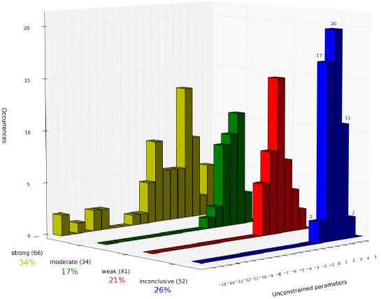
V.6 Reheating

Figure 21: The quantity $\Delta\pi_{\ln R_{\mathrm{reh}}}/\Delta\mathcal{P}_{\ln R_{\mathrm{reh}}}$, quantifying how much the reheating is constrained, versus the Bayesian evidence for Encyclopaedia Inflationaris models (each model is represented by a circle the size of which has no meaning). The inset shows the posterior distribution of the reheating parameter for the ten best Planck 2013 models. Figure taken from Ref. Martin et al. (2014c).

Figure 22: Same as in Fig. 21 but assuming the mean equation of state during reheating is known. The prior-to-posterior width for the reheating energy density $\ln(\rho_{\mathrm{reh}}/M_{\scriptscriptstyle{\mathrm{Pl}}}^{4})$ is represented assuming four values of the mean equation of state $\overline{w}_{\mathrm{reh}}$, namely $\overline{w}_{\mathrm{reh}}=-0.3$ (top left panel), $\overline{w}_{\mathrm{reh}}=-0.2$ (top right panel), $\overline{w}_{\mathrm{reh}}=0$ (bottom left panel) and $\overline{w}_{\mathrm{reh}}=0.2$ (bottom right panel). Figures taken from Ref. Martin et al. (2014c).

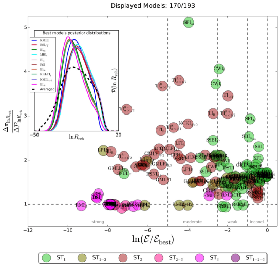
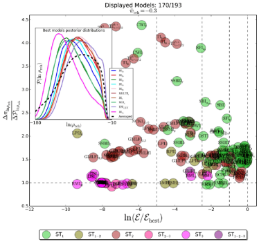
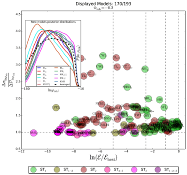
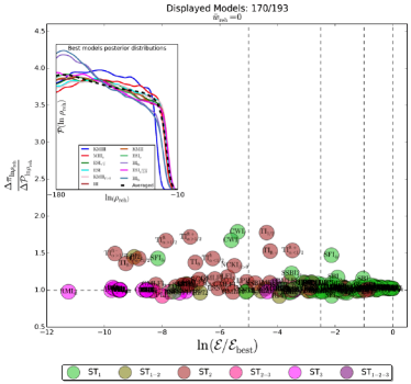
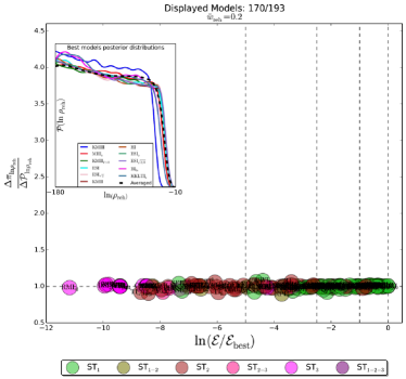
We now describe the constraints on reheating that can be inferred from the Planck 2013 data. This question was recently studied in Ref. Martin et al. (2014c). In Sec. III.3, we have seen that, as far as CMB data are concerned, reheating can be entirely described by the parameter $R_{\mathrm{rad}}$, see Eq. (1.71) or, equivalently, $R_{\mathrm{reh}}$, see Eq. (1.70). For each inflationary model, Ref. Martin et al. (2014c) has calculated the posterior distribution of the parameter $\ln R_{\mathrm{reh}}$. In order to estimate how much reheating is constrained, it is convenient to introduce the ratio $\Delta\pi_{\ln R_{\mathrm{reh}}}/\Delta\mathcal{P}_{\ln R_{\mathrm{reh}}}$. In this formula, $\Delta\pi_{\ln R_{\mathrm{reh}}}$ is the standard width of the prior while $\Delta\mathcal{P}_{\ln R_{\mathrm{reh}}}$ is the standard width of the posterior distribution. Therefore if $\Delta\pi_{\ln R_{\mathrm{reh}}}/\Delta\mathcal{P}_{\ln R_{\mathrm{reh}}}=1$, the posterior is as wide as the prior and reheating is not constrained at all. If, however, $\Delta\pi_{\ln R_{\mathrm{reh}}}/\Delta\mathcal{P}_{\ln R_{\mathrm{reh}}}>1$, then the posterior distribution is more peaked than the prior and there is information gain. Clearly, the larger the ratio $\Delta\pi_{\ln R_{\mathrm{reh}}}/\Delta\mathcal{P}_{\ln R_{\mathrm{reh}}}$, the more peaked the posterior.

The prior on $\ln R_{\mathrm{reh}}$ has to be chosen carefully and must be justified by physical considerations. Clearly, the energy density at the end of reheating must be smaller than that at the end of inflation and larger than at the BBN time where $\rho_{\rm nuc}=\left(10\mathrm{MeV}\right)^{4}$. Therefore, we require $\rho_{\rm nuc}<\rho_{\rm reh}<\rho_{\rm end}$. For the mean equation of state, we take $-1/3<\overline{w}_{\mathrm{reh}}<1$ since, by definition, reheating is a non accelerated phase of expansion. As a consequence, one can show that this leads to

$$\ln\left(\frac{\rho_{\rm nuc}^{1/4}}{M_{\scriptscriptstyle{\mathrm{Pl}}}}\right)<\ln R_{\mathrm{reh}}<\ln\left(\frac{\rho_{\rm nuc}^{1/4}}{M_{\scriptscriptstyle{\mathrm{Pl}}}}\right)+\frac{4}{3}\ln\left(\frac{\rho_{\rm end}^{1/4}}{M_{\scriptscriptstyle{\mathrm{Pl}}}}\right).$$ (1.285)

The order of magnitude of $R_{\mathrm{reh}}$ being unknown, we choose a Jeffreys prior in the above range. Notice that this differs from what was done in the Planck 2013 paper Ade et al. (2013b). Indeed, in that work, specific reheating scenarios were considered such as instantaneous reheating or “restrictive reheating” where, apparently without a strong justification, the reheating energy density is fixed to $10^{9}\mathrm{GeV}$. Moreover, it seems that a prior on the quantity $\Delta N_{*}$ was chosen which is clearly awkward since it does not necessarily guarantee that the two physical conditions on $\rho_{\rm reh}$ and $\overline{w}_{\mathrm{reh}}$ discussed previously are valid. In the Planck $2015$ paper Ade et al. (2015a), it seems that this weird approach has been given up. The new method now seems closer to what is done in the present article. Notice, however, that, if the prior on the reheating energy density appears reasonable, only specific values of $\overline{w}_{\mathrm{reh}}$ are considered which is, of course, not the most general case. Let us also remark that Ref. Ade et al. (2015a) introduces an equation of state parameter during reheating, denoted $w_{\rm int}$, called the “effective equation of state” but without defining it precisely. In particular, it is difficult to know if it is equal to the parameter introduced in Eq. (1.64), which is the correct parameter that ought to be used and was introduced for the first time in Ref. Martin and Ringeval (2010).

In Fig. 21, we have represented each Encyclopaedia Inflationaris model in the space $\left(\Delta\pi_{\ln R_{\mathrm{reh}}}/\Delta\mathcal{P}_{\ln R_{\mathrm{reh}}},\ln B^{i}_{{\scriptscriptstyle{\mathrm{REF}}}}\right)$: good models are on the right and models for which reheating is constrained are on the top. The horizontal dashed line $\Delta\pi_{\ln R_{\mathrm{reh}}}/\Delta\mathcal{P}_{\ln R_{\mathrm{reh}}}=1$ locates the models for which reheating is not constrained. In order to globally assess the value of the constraints, we can define the following quantity

$$\left\langle\frac{\Delta\pi_{\ln R_{\mathrm{reh}}}}{\Delta\mathcal{P}_{\ln R_{\mathrm{reh}}}}\right\rangle\equiv\frac{1}{\sum_{j}\mathcal{E}_{j}}\displaystyle\sum_{i}\mathcal{E}_{i}\left(\frac{\Delta\pi_{\ln R_{\mathrm{reh}}}}{\Delta\mathcal{P}_{\ln R_{\mathrm{reh}}}}\right)_{i},$$ (1.286)

which is the mean value of $\Delta\pi_{\ln R_{\mathrm{reh}}}/\Delta\mathcal{P}_{\ln R_{\mathrm{reh}}}$ weighted by the Bayesian evidence, i.e. the mean value in the space of models. This is a fair estimate since disfavored models will not contribute a lot to this quantity due to their small evidence. Numerically, the Planck 2013 data are such that

$$\left\langle\frac{\Delta\pi_{\ln R_{\mathrm{reh}}}}{\Delta\mathcal{P}_{\ln R_{\mathrm{reh}}}}\right\rangle\simeq 1.66$$ (1.287)

which, therefore, indicates that reheating is indeed constrained.

It is also interesting to assume that the mean equation of state is known. In that case, the parameter $R_{\mathrm{reh}}$ only depends on the energy density at the end of reheating or, equivalently, on the reheating temperature. In Fig. 22, we have represented the similar quantities as in Fig. 21 for four different values of $\overline{w}_{\mathrm{reh}}$, namely $\overline{w}_{\mathrm{reh}}=-0.3,-0.2,0,0.2$. The most striking feature of this plot is that, for positive values of $\overline{w}_{\mathrm{reh}}$, the models tend to cluster around the horizontal line $\Delta\pi_{\ln R_{\mathrm{reh}}}/\Delta\mathcal{P}_{\ln R_{\mathrm{reh}}}=1$. This indicates that, for those values of the mean equation of state, reheating is not constrained. As a consequence, the number obtained in Eq. (1.287) comes in fact from a region in parameter space where $\overline{w}_{\mathrm{reh}}<0$. This conclusion makes sense since, for $\overline{w}_{\mathrm{reh}}<0$, the dispersion of the predictions in the $(r,n_{\scriptscriptstyle{\mathrm{S}}})$ space is much bigger than for positive equation of state. More details can be found in Ref. Martin et al. (2014c), in particular concrete bounds on the reheating temperature for different models.

Concluding, the reheating phase is already constrained by the Planck $2013$ data. The precise values of the allowed reheating temperatures depend on the model under consideration and on the mean equation of state. If $\overline{w}_{\mathrm{reh}}>0$, the constraints are very mild. It is also worth noticing that two identical models with two different reheating histories can have different Bayesian evidence. This means that, given the accuracy of the CMB measurements, reheating now needs to be properly included in data analysis.

VI Conclusion

In this last section, we briefly summarize what we have learned about inflation in the recent years. Inflation is a “violent” phenomenon since it could occur at energies as high as the Grand Unified Theory scale, i.e. $\sim 10^{16}$ GeV. It is thus quite remarkable to be able to say something about physics at such a high energy scale. The picture that seems to emerge from the recent high accuracy astrophysical measurements is that inflation is realized in its simplest version, namely single-field slow-roll with a minimal kinetic term. Additional features, such as the presence of several fields or non-minimal kinetic term, which may appear as (natural) consequences of embedding inflation in high energy physics, do not seem to be relevant. If, indeed, inflation is really realized in its vanilla version, an important challenge will be (is) to understand, from the high energy point of view, why these extra ingredients are in fact not present. Also, important questions such as the physical nature of the inflaton field remains unanswered.

The shape of the potential is also constrained and appears to be of the “plateau shape”, a typical example of this class of scenarios being the Starobinsky model. Popular models such as monomial potentials are now disfavored.

Interestingly enough, inflationary reheating is also constrained by the Planck data. The constraints are model dependent and correspond to an average reduction of the prior-to-posterior of about $40\%$.

Given this situation, what should be done to increase our knowledge of inflation? It is clear that in order to measure more precisely the shape of the potential, one needs to constrain the values of the Hubble flow parameters $\epsilon_{n}$. So far, we only have a good measurement of the scalar spectral index which is a specific combination of $\epsilon_{1}$ and $\epsilon_{2}$, namely $n_{\scriptscriptstyle{\mathrm{S}}}=1-2\epsilon_{1}-\epsilon_{2}$. To measure $\epsilon_{1}$ and $\epsilon_{2}$ separately, one needs another observable. A more accurate measurement of the scalar power spectrum cannot really do the job since it involves an additional parameter, $\epsilon_{3}$, see Eq. (1.265). We are therefore left with either the tensor-to-scalar ratio $r$, which is directly proportional to $\epsilon_{1}$, see Eq. (1.87), or the bispectrum which depends on $\epsilon_{1}$ and $\epsilon_{2}$ in a different combination than the spectral index, see Eq. (1.253) and Eqs. (1.249), (1.250), (1.251) and (1.252).

Measuring primordial Non-Gaussianities has one great advantage: we already know in advance where one should find the signal. If one dares an analogy, it is like searching for the Higgs boson. We know that if it is not found in a specific window, the consequences would be drastic. However, the shortcomings is that the amplitude of the signal, $f_{{}_{\mathrm{NL}}}\simeq 0.01$, is so small that it is not clear whether it is technologically feasible. On the other hand, improving the limits on Non-Gaussianities could be very rewarding. Many non-vanilla scenarios predict $f_{{}_{\mathrm{NL}}}\simeq 1$ and reaching this limit could allow us to rule out single field slow-roll models!

Measuring the tensor-to-scalar ratio is the other possibility. It requires to measure the tensor contribution which can be done through a detection of $B$-mode CMB polarization. At the moment, there are considerable efforts in this direction. The first claim of a detection of primordial gravity waves was of course made by the BICEP2 team Ade et al. (2014a). The signal corresponds to a tensor-to-scalar ratio of $r\sim 0.16$. However, as later shown by the Planck team and already discussed before, the signal can probably be entirely explained by dust emission Ade et al. (2014b). Other ground based experiments are currently operating in Antarctica such as BICEP3 & Keck (three channels: $100$ GHz, $150$ GHz and $200$ GHz, sky coverage of $1-2\%$ and resolution of $30^{\prime}$), SPTPol/SPT₃G ($90$ GHz and $150$ GHz, $6\%$, $1.2^{\prime}$), in Chile such as Atacama B-mode Search (ABS) ($145$ GHz, $2\%$, $30^{\prime}$), Atacama Cosmology Telescope (ACTPol)/AdvACT ($30$ GHz, $40$ GHz, $90$ GHz, $150$ GHz and $230$ GHz, $6\%$, $1.4^{\prime}$), POLARBEAR/SIMONS ($90$ GHz, $150$ GHz and $220$ GHz, $6\%$, $3-5^{\prime}$) and in the Canary islands such as QUIJOTE ($11-20$ GHz and $30$ GHz, $65\%$, $15^{\prime}-55^{\prime}$). Soon ($2016$) in Chile, the experiment Cosmology Large Scale Surveyor (CLASS) ($40$ GHz, $90$ GHz and $150$ GHz, $70\%$) will start taking data. There are also balloon borne experiments such as EBEX ($150$ GHz, $250$ GHz and $410$ GHz, $8\%$, $10^{\prime}$) and SPIDER ($90$ GHz, $150$ GHz and $280$ GHz, $8\%$, $30^{\prime}-40^{\prime}$) which are operating in Antarctica and Primordial Inflation Polarization Explorer (PIPER) ($200$ GHz, $270$ GHz, $350$ GHz and $600$ GHz, $70\%$, $10^{\prime}-20^{\prime}$) which will be starting in $2016$ in Palestine in USA (Texas). The most efficient of these experiments will reach a level corresponding to $r\sim 0.01$ in the following $3-5$ years. If one wants to go further, one needs space missions. Two projects appear to be particularly promising: the Lite satellite for the studies of $B$-modes polarization and Inflation from cosmic background Radiation Detection (LiteBIRD) Matsumura et al. (2013) selected as one of the prioritized projects in the master plan $2014$ by the Science Council of Japan and the Cosmic Origins Explorer (COrE+) The COrE Collaboration et al. (2011) which is a proposal for European Space Agency (ESA) M4 space mission. LiteBIRD has a polarization sensitivity of $\sim 4.5\mu\mbox{K}\times\mbox{arcmin}$, a resolution of $\theta_{\rm fwhm}=38.5^{\prime}$ and a sky coverage of $70\%$. COrE+ can be “light” with a sensitivity of $\sim 2.5\mu\mbox{K}\times\mbox{arcmin}$ and a resolution of $\theta_{\rm fwhm}=6^{\prime}$ or “extended” with a sensitivity of $\sim 1.5\mu\mbox{K}\times\mbox{arcmin}$ and a resolution of $\theta_{\rm fwhm}=4^{\prime}$ (in both cases, the sky coverage is $70\%$). With these space missions, one should be able to gain one order of magnitude on $r$ and reach $r\sim 10^{-3}$ in the next decade, assuming no delensing. With delensing, one might be able to probe even smaller values of $r$.

Using the above analogy, measuring $r$ is like searching for super-symmetry. We do not know at which level it should show up (we do not know the super-symmetry breaking scale) but it could be around the corner and, hence, technologically realistic. In fact, a determination of $r$ would immediately lead to the inflaton field excursion. An excursion which is just Planckian corresponds to a tensor-to-scalar ratio of $r\sim 10^{-3}$ that is to say precisely the limit reached by future space missions. Therefore, given that $r=16\epsilon_{1}$, if $\epsilon_{1}\gtrsim 10^{-4}$, then one should be able to measure it in the next decade.

Of course, a detection of primordial gravity waves would also impact model comparison. It was recently shown in Ref. Martin et al. (2014f) that this could allow us to rule out almost three-quarters of the inflationary models compared to one-third for Planck $2013$.

In conclusion, detecting $B$-mode CMB polarization and, hence, primordial gravity waves, is probably the next challenge for primordial Cosmology. An additional step would then be to check the consistency relation, $r=-8n_{\scriptscriptstyle{\mathrm{T}}}$, which would constitute the final proof that vanilla inflation occurred in the early Universe. However, if $r$ is very small, this measurement might be too difficult. In any case, at the time of writing, detecting primordial gravity waves appears to be the next frontier for inflation. Only time will tell whether this is true or not.