Long-Range Spin-Triplet Correlations and Edge Spin Currents in Diffusive Spin-Orbit Coupled $SNS$ Hybrids with a Single Spin-Active Interface

Abstract

Utilizing a SU(2) gauge symmetry technique in the quasiclassical diffusive regime, we theoretically study finite-sized two-dimensional intrinsic spin-orbit coupled superconductor/normal-metal/superconductor ($S$/$N$/$S$) hybrid structures with a single spin-active interface. We consider intrinsic spin-orbit interactions (ISOIs) that are confined within the $N$ wire and absent in the $s$-wave superconducting electrodes ($S$). Using experimentally feasible parameters, we demonstrate that the coupling of the ISOIs and spin moment of the spin-active interface results in maximum singlet-triplet conversion and accumulation of spin current density at the corners of the $N$ wire nearest the spin-active interface. By solely modulating the superconducting phase difference, we show how the opposing parities of the charge and spin currents provide an effective venue to experimentally examine pure edge spin currents not accompanied by charge currents. These effects occur in the absence of externally imposed fields, and moreover are insensitive to the arbitrary orientations of the interface spin moment. The experimental implementation of these robust edge phenomena are also discussed.

I Introduction

The interaction of a moving particles’ spin with its linear momentum embodies the so-called spin-orbit interaction (SOI). The SOI is a quantum mechanical effect that is relativistic in origin. For materials possessing a strong SOI effect, it becomes possible to manipulate spin currents with less dissipation, higher speeds, and lower power consumption compared to conventional charge-based devices kikkawa_1 . Consequently, a number of high-performance devices that exploit the SOI effect have been proposed, including, spin transistors, and devices that store or transport information wolf_1 ; stepanenko_1 ; rashba_book_1 ; Wunderlich_1 ; Miron_1 . The types of SOIs can be categorized as follows: $i)$ intrinsic (originating from the electronic band structure of the material) and $ii)$ extrinsic (originating from the spin-dependent scattering from impurities) zhang_1 . Of particular interest are intrinsic SOIs (ISOIs), due to their controllability by tuning a gate voltage rashba_book_1 ; nagaosa_1 ; winklwer_1 ; awschalom_1 ; Miron_1 ; Erlingsson ; tanaka_2 . Two commonly studied ISOIs are the Rashba and Dresselhaus types. The Rashba SOI rashba_book_1 can be described via spatial inversion asymmetries, while the Dresselhaus SOI dresselhaus_term is a result of bulk inversion asymmetries within the crystal structure winklwer_1 ; rashba_book_1 .

There have also been extensive efforts to manipulate the spin currentsprinz_1 ; wolf_1 ; zhang_1 ; kikkawa_1 ; Demidov in SOI systems via the spin Hall effect Murakami_1 ; hirsh_1 ; kato_1 ; Sinova_1 ; mishchenko_1 ; chazalviel ; Nikolic ; malsh_severin , and the quantum spin Hall effect Hasan_1 ; Qi_1 . Since spin currents are weakly sensitive to nonmagnetic impurities and temperature zhang_1 , more opportunities arise in the development of high speed low-dissipative spintronic devices kikkawa_1 . Along these lines, superconducting heterostructures have been making strides as potential platforms where spin-orbit coupling (SOC) plays a key role, including scenarios involving the spin-Hall effect malsh_sns ; malsh_severin ; malsh_3 ; reynoso_1 ; ex_so_JJ ; Konschelle ; yokoyama ; tanaka_2 ; bobkova_1 ; arahata_1 ; buzdin_so_ext ; golubov_rmp ; buzdin_rmp ; niu_1 ; wu_1 ; bergeret_so . When considering superconducting hybrids with SOC, interface phenomena at superconducting junctions becomes particularly important. For example, the interface of a hybrid superconducting junction can behave as a spin-polarizer when it is coated by an ultrathin uniform $F$ layer. The study of interface effects that involve spin-dependent scattering spnactv_1 ; spnactv_6 ; spnactv_8 has spanned considerable theoretical spnactv_12 ; spnactv_6 ; spnactv_1 ; spnactv_21 ; spnactv_16 ; spnactv_12 ; spnactv_14 ; spnactv_15 ; spnactv_16 ; spnactv_20 ; spnactv_21 and experimental works Tedrow ; DOS_1_ex ; DOS_2_ex . Advancements in nanofabrication and theoretical techniques involving superconducting hybrids with spin-active interfaces have thus created new venues for controlling superconducting pair correlations, spin currents, and majorana fermions spnactv_1 ; spnactv_6 ; spnactv_8 ; spnactv_12 ; spnactv_14 ; spnactv_15 ; spnactv_16 ; spnactv_20 ; spnactv_21 ; nayana .

To explore the interplay of these phenomena, we consider charge and spin currents in a finite sized intrinsic spin-orbit coupled $s$-wave superconductor/normal-metal/$s$-wave superconductor ($S$/$N$/$S$) junction with a single spin-active interface. We utilize a spin-parameterized two-dimensional Keldysh-Usadel technique bergeret_so in the presence of ISOIs. In order to theoretically account for spin-polarization and spin-dependent phase shifts that a quasiparticle experiences upon transmitting across spin-active interfaces, spin-boundary conditions are utilized spnactv_12 . The spin-parametrization scheme allows us to isolate the spin-singlet and spin-triplet correlations, and pinpoint their spatial behavior. We find that the combination of interface spin moment and ISOIs results in triplet pairings with $m=0,\pm 1$ spin projections along the quantization axis bergeret1 ; buzdin_rmp ; golubov_rmp ; halterman1 ; alid_1 ; alid_2 ; alid_3 . We also find that maximum singlet-triplet conversion and spin-current densities takes place at the corners of the $N$ wire nearest the spin-active interface, where the spin accumulation is greatest. The spin currents possess three nonzero spin components, independent of either the actual type of ISOI present in the $N$ wire or spin moment orientation of the $S$/$N$ spin-active interface. When comparing the spin and charge currents as functions of the superconducting phase difference, $\varphi$, we show that current phase relations for the charge supercurrents are typically governed by sinusoidal-like, odd functions in $\varphi$, although anomalous behavior buzdin_phi0 ; yokoyama ; Konschelle can arise. The spin currents however, are even functions of $\varphi$ma_kh_njp . These opposing behaviors of the spin and charge currents present a simple and experimentally feasible platform to effectively generate proximity-induced spin-triplet superconducting pairings and edge spin currents in the absence of any charge supercurrent. It was demonstrated in Ref. ma_kh_njp, that the combination of spontaneously broken time-reversal symmetry and lack of inversion symmetry can result in spontaneously accumulated spin currents at the edges of finite-size two-dimensional magnetic $S$/$F$ hybrids. Moreover, we describe experimentally accessible signatures in the physically relevant quantities, and discuss realistic material parameters and geometrical configurations that lead to the edge spin effects predicted here. Our proposed hybrid structure, based on its intrinsic properties alone, can be viewed as a simpler alternative to differing systems that rely inextricably on externally imposed fields to generate the desired edge spin currents Murakami_1 ; hirsh_1 ; kato_1 ; Sinova_1 ; mishchenko_1 ; chazalviel ; Nikolic ; malsh_sns ; malsh_severin .

The paper is organized as follows: We outline the theoretical techniques and approximations used to characterize the intrinsic spin-orbit coupled superconducting $S$/$N$/$S$ hybrid structures with spin-active interfaces in Sec. II. In Sec. III, we discuss all of the types of superconducting pairings present (spin-singlet and spin-triplet correlations) and illustrate the associated spatial profiles, which follow directly from the inherent proximity effects. Next, we present results for the spin current densities, with spatial maps, and discuss possible experimental realizations of the presented edge spin phenomena. In addition, we discuss the spin current symmetries relative to the spin moment orientation of the spin-active interface in the presence of Rashba or Dresselhaus SOC. We finally summarize our findings in Sec. IV.

II Theoretical formalism

A quasiclassical framework has recently been developed for superconducting hybrid structures in the presence of generic spin-dependent fieldsbergeret_so . These generic fields can be reduced to ISOIs, such as, Rashbarashba_term and Dresselhausdresselhaus_term , in terms of the quasiparticles’ linear momentum [${\bm{p}}=(p_{x},p_{y},p_{z})$]. If we define a vector of Pauli matrices ${\bm{\tau}}=(\tau_{x},\tau_{y},\tau_{z})$ (see Appendix A), the corresponding Hamiltonians describing these ISOIs can be straightforwardly expressed as,

$$\mathcal{H}_{\text{R}}=\Omega_{\text{R}}({\bm{p}}\times{\bm{\tau}})\cdot\hat{{\bm{z}}}\;\mathop{\overset{\mathrm{p_{z}=0}}{\leavevmode\resizebox{0.0pt}{0.0pt}{=}}}\;\Omega_{\text{R}}(p_{x}\tau^{y}-p_{y}\tau^{x}),$$

$$\mathcal{H}_{\text{D}}=\Omega_{\text{D}}({\bm{p}}\cdot{\bm{\tau}})\;\;\;\;\;\;\;\mathop{\overset{\mathrm{p_{z}=0}}{\leavevmode\resizebox{0.0pt}{0.0pt}{=}}}\;\Omega_{\text{D}}(p_{x}\tau^{x}+p_{y}\tau^{y}),$$

where the momentum is restricted to the $xy$ plane. The R and D indices represent the Rashba and Dresselhaus SOIs with strength $\Omega_{\text{R}}$ and $\Omega_{\text{D}}$, respectively. A linearized ISOI can be treated as an effective background field that obeys the SU(2) gauge symmetries. bergeret_so ; gorini_1 ; gorini_3 ; Konschelle Therefore, to incorporate ISOIs into the quasiclassical approach, it is sufficient for partial derivatives to be interchanged with their covariants. bergeret_so ; gorini_1 ; Konschelle This simple prescription is one of the advantages of the SU(2) approach, besides the convenient definitions of physical quantities such as the spin currents.duckheim_1 ; gorini_3

A description of quasiparticle transport inside a superconducting medium is provided by the Dyson equation. Eilenberger The corresponding equation of motion in the quasiclassical approximation for clean systems reduces to the so-called Eilenberger equationEilenberger . The Eilenberger equation can be further reduced to a simpler set of equations in the diffusive regime, where the quasiparticles are scattered into random directions. This permits integration of the Eilenberger equation over all possible momentum directions, yielding a simpler picture for highly impure systems, as first introduced by Usadel Usadel .

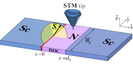
Figure 1: (Color online) Schematic of a two-dimensional $S$/$N$/$S$ Josephson junction with a spin-active interface at $x=0$ described by ${\bf S}_{l}=(S_{l}^{x},S_{l}^{y},S_{l}^{z})$. The intrinsic spin-orbit coupled normal-metal strip ($N$) is of length and width $d_{N}$, and $W_{N}$, respectively. The superconducting electrodes ($Sc$), however, are SOI-free and connected to the $N$ wire at $x=0$, and $x=d_{N}$. The two-dimensional junction resides in the $xy$ plane so that the $S$/$N$ interfaces are parallel with the $y$ axis. The cone depicts the tip of a scanning tunneling microscope (STM) that can sweep the entire surface of the $N$ layer in the $xy$ plane.

The resultant Usadel equation is the central equation used in this paper, and can be expressed compactly as bergeret1 ; Usadel ; bergeret_so :

$$\mathfrak{D}\Big{[}{\bm{\partial}},{G}({\bm{r}},\varepsilon)[{\bm{\partial}},{G}({\bm{r}},\varepsilon)]\Big{]}+i[\varepsilon{\rho}_{3}-\Delta,{G}({\bm{r}},\varepsilon)]=0,$$ (1)

where ${\rho}_{3}$ is a $4\times 4$ Pauli matrix (see Appendix A), $\mathfrak{D}$ represents the diffusion constant, and $\Delta$ is a $4\times 4$ matrix which represents the superconducting gap alid_3 . We denote the quasiparticle energy by $\varepsilon$, relative to the Fermi energy, $\varepsilon_{F}$. In the superconducting leads, the Usadel equation, Eq. (1), is solved in the presence of $\Delta$ which results in the BCS bulk solution given by Eq. (20). Within the nonsuperconducting region however, $\Delta=0$, and the boundary conditions, Eq. (II), should be simultaneously satisfied. The total Green’s function for the system, $G({\bm{r}},\varepsilon)$, is comprised of the Advanced ($G^{R}({\bm{r}},\varepsilon)$), Retarded ($G^{A}({\bm{r}},\varepsilon)$), and Keldysh ($G^{K}({\bm{r}},\varepsilon)$) propagators:

$$G({\bm{r}},\varepsilon)=\left[\begin{array}[]{cc}G^{R}({\bm{r}},\varepsilon)&G^{K}({\bm{r}},\varepsilon)\\ 0&G^{A}({\bm{r}},\varepsilon)\end{array}\right];$$ (4)

$$G^{A}({\bm{r}},\varepsilon)=\left[\begin{array}[]{cc}-\mathcal{G}({\bm{r}},-\varepsilon)&-\mathcal{F}({\bm{r}},-\varepsilon)\\ \mathcal{F}^{*}({\bm{r}},\varepsilon)&\mathcal{G}^{*}({\bm{r}},\varepsilon)\end{array}\right].$$ (7)

Since we consider the low proximity limit of the diffusive regime, bergeret1 , the normal and anomalous components of the Green’s function can be approximated by, $\mathcal{G}({\bm{r}},\varepsilon)\simeq 1$ and $\mathcal{F}({\bm{r}},\varepsilon)\ll 1$, respectively. Thus the advanced component of total Green’s function reduces to:

$${G}^{A}({\bm{r}},\varepsilon)\approx\left[\begin{array}[]{cc}-1&-\mathcal{F}({\bm{r}},-\varepsilon)\\ \mathcal{F}^{\ast}({\bm{r}},\varepsilon)&1\\ \end{array}\right].$$ (10)

Within the low proximity approximation, the advanced component can be ultimately expressed as:

$${G}^{A}({\bm{r}},\varepsilon)=$$

$$\left[\begin{array}[]{cccc}-1&0&-f_{\upuparrows}({\bm{r}},-\varepsilon)&-f_{-}({\bm{r}},-\varepsilon)\\ 0&-1&-f_{+}({\bm{r}},-\varepsilon)&-f_{\downdownarrows}({\bm{r}},-\varepsilon)\\ f_{\upuparrows}^{\ast}({\bm{r}},\varepsilon)&f_{-}^{\ast}({\bm{r}},\varepsilon)&1&0\\ f_{+}^{\ast}({\bm{r}},\varepsilon)&f_{\downdownarrows}^{\ast}({\bm{r}},\varepsilon)&0&1\\ \end{array}\right].$$ (15)

In equilibrium, the Retarded and Keldysh blocks of the total Green’s function are obtained via: ${G}^{A}({\bm{r}},\varepsilon)=-\big{\{}\hat{\rho}_{3}{G}^{R}({\bm{r}},\varepsilon)\hat{\rho}_{3}\big{\}}^{{\dagger}}$, and ${G}^{K}({\bm{r}},\varepsilon)=\tanh(\varepsilon k_{B}\mathcal{T}/2)\big{\{}{G}^{R}({\bm{r}},\varepsilon)-{G}^{A}({\bm{r}},\varepsilon)\big{\}}$. The Boltzmann constant and system temperature are denoted by $k_{B}$ and $\mathcal{T}$, respectively. Within the low proximity approximation, the linearized Usadel equation involves sixteen coupled complex partial differential equations which become even more complicated in the presence of ISOI terms. Unfortunately, the resultant system of coupled differential equations can be simplified and decoupled only in extreme limits that can be experimentally unrealistic.golubov_rmp ; buzdin_rmp ; bergeret1 When such simplifications are made, the equations lead to analytical expressions for the Green’s function componentsalidoust_4termin . For the complicated system considered in this paper however, computational methods are the most efficient, and sometimes only possible routes to investigate experimentally accessible transport properties.bergeret_so

The complex partial differential equations must be supplemented by the appropriate boundary conditions to properly describe the spin and charge currents in spin-orbit coupled $S$/$N$/$S$ hybrids with spin-active interfaces:cite:zaitsev ; spnactv_12

$$\zeta\big{\{}{G}({\bm{r}},\varepsilon){\bm{\partial}}{G}({\bm{r}},\varepsilon)\big{\}}\cdot{\bm{n}}=[{G}_{\text{BCS}}(\theta_{lr},\varepsilon),{G}({\bm{r}},\varepsilon)]$$

$$\pm i[{\bm{S}}_{lr}\cdot{\bm{\nu}},{G}({\bm{r}},\varepsilon)],$$ (16)

where the unit vector, ${\bm{n}}$, is directed normal to an interface, and it is assumed for the time being that the left and right interfaces [Fig. 1] are spin-active. The leakage intensity of superconducting correlations from the $S$ electrodes to the $N$ wire is controlled by the ratio between the resistance of the barrier region $R_{B}$ and the resistance in the normal layer $R_{N}$: $\zeta=R_{B}/R_{N}$.alidoust_1

We describe the spin moments of the left ($l$) and right ($r$) interfaces by two generic vectors as follows:spnactv_1 ; spnactv_6

$${\bm{S}}_{lr}=(S_{lr}^{x},S_{lr}^{y},S_{lr}^{z}),$$ (17)

where the ${\bm{S}}_{lr}$ can have arbitrary directions and magnitude of the spin moment at the $S$/$N$ interfaces. The solution to Eq. (1) for a bulk even-frequency $s$-wave superconductor results in

$${G}^{R}_{\text{BCS}}(\theta,\varepsilon)=\left[\begin{array}[]{cc}\sigma^{0}\cosh\vartheta(\varepsilon)&i\sigma^{y}e^{i\theta}\sinh\vartheta(\varepsilon)\\ i\sigma^{y}e^{-i\theta}\sinh\vartheta(\varepsilon)&-\sigma^{0}\cosh\vartheta(\varepsilon)\\ \end{array}\right],$$ (20)

where $\vartheta(\varepsilon)=\text{arctanh}({|\Delta|}/{\varepsilon})$, and $\theta$ represents the macroscopic phase of the bulk superconductor. The phase difference between the left and right $S$ electrodes, shown in Fig. 1, is denoted $\theta_{l}-\theta_{r}=\varphi$. We define $s$ and $c$ terms in the superconducting bulk solution, ${G}_{\text{BCS}}^{R}$, by piecewise functions:

$$s(\varepsilon)\equiv e^{i\theta}\sinh\vartheta(\varepsilon)=$$

$$-\Delta\left\{\frac{\text{sgn}(\varepsilon)}{\sqrt{\varepsilon^{2}-\Delta^{2}}}\Theta(\varepsilon^{2}-\Delta^{2})-\frac{i}{\sqrt{\Delta^{2}-\varepsilon^{2}}}\Theta(\Delta^{2}-\varepsilon^{2})\right\},$$

$$c(\varepsilon)\equiv\cosh\vartheta(\varepsilon)=$$

$$\frac{\mid\varepsilon\mid}{\sqrt{\varepsilon^{2}-\Delta^{2}}}\Theta(\varepsilon^{2}-\Delta^{2})-\frac{i\varepsilon}{\sqrt{\Delta^{2}-\varepsilon^{2}}}\Theta(\Delta^{2}-\varepsilon^{2}),$$

where $\Theta(x)$ is the Heaviside step function and $\Delta$ is the superconducting gap at temperature $\mathcal{T}$ for a conventional $s$-wave superconductor.

We next employ a spin-dependent field technique that permits the incorporation of ISOIs into the Keldysh-Usadel approachbergeret_so . As stated earlier, this technique has been widely used in the literature gorini_1 ; gorini_3 ; mishchenko_1 ; malsh_sns ; Konschelle and was most recently extended for superconducting heterostructuresbergeret_so . In much the same spirit, we adopt a generic tensor vector potential ${\bm{A}}({\bm{r}})=\big{(}A_{x}({\bm{r}}),A_{y}({\bm{r}}),A_{z}({\bm{r}})\big{)}$:bergeret_so ; gorini_1 ; gorini_3 ; ma_kh_njp

$$A_{x}({\bm{r}})=\frac{1}{2}\Big{\{}\mathcal{A}_{x}^{x}({\bm{r}})\tau^{x}+\mathcal{A}_{x}^{y}({\bm{r}})\tau^{y}+\mathcal{A}_{x}^{z}({\bm{r}})\tau^{z}\Big{\}},$$ (21a)

$$A_{y}({\bm{r}})=\frac{1}{2}\Big{\{}\mathcal{A}_{y}^{x}({\bm{r}})\tau^{x}+\mathcal{A}_{y}^{y}({\bm{r}})\tau^{y}+\mathcal{A}_{y}^{z}({\bm{r}})\tau^{z}\Big{\}},$$ (21b)

$$A_{z}({\bm{r}})=\frac{1}{2}\Big{\{}\mathcal{A}_{z}^{x}({\bm{r}})\tau^{x}+\mathcal{A}_{z}^{y}({\bm{r}})\tau^{y}+\mathcal{A}_{z}^{z}({\bm{r}})\tau^{z}\Big{\}}.$$ (21c)

We can now define the covariant derivative by,

$${\bm{\partial}}\equiv\vec{\partial}\hat{1}-ie{\bm{A}}({\bm{r}}),$$ (22)

where $\vec{\partial}\equiv(\partial_{x},\partial_{y},\partial_{z})$. Hence, the brackets in the Usadel equation Eq. (1) and the boundary conditions Eq. (II) (as well as the charge and spin currents discussed below) are equivalent to:

$$[{\bm{\partial}},{G}({\bm{r}})]=\vec{\partial}{G}({\bm{r}})-ie[{\bm{A}}({\bm{r}}),{G}({\bm{r}})].$$ (23)

It should be noted that the quasiclassical approach employed here allows for the study of systems with spin dependent vector potentials possessing arbitrary spatial patterns, and spin-active interfaces with arbitrary spin moment directions. Here we assume that the impurity scattering (encapsulated by the diffusion constant) is spin-independent, and thus the spin-dependent fields introduced in Eqs. (21) describe the spin-orbit coupling for the system. Within the quasiclassical approximation, the quasiparticles’ momentum is localized around the Fermi level. Therefore, the spin moment amplitude for spin-active interfaces $|{\bm{S}}_{l,r}|$, the vector potential, $|{\bm{A}}|$, and superconducting gap $|\Delta|$, should all be appropriately smaller than the Fermi energy $\varepsilon_{F}$ bergeret_so .

A specific choice of the tensor vector potentialgorini_1 [Eq. (21)] that results in linearized Rashba ($\alpha\neq 0,\beta=0$) rashba_term and Dresselhaus ($\beta\neq 0,\alpha=0$) dresselhaus_term SOCs is:

$$\left\{\begin{array}[]{l}\mathcal{A}_{x}^{x}=-\mathcal{A}_{y}^{y}=2\beta,\\ \mathcal{A}_{x}^{y}=-\mathcal{A}_{y}^{x}=2\alpha,\\ \hline\cr\mathcal{A}_{x}^{z}=\mathcal{A}_{y}^{z}=0,\\ \mathcal{A}_{z}^{z}=\mathcal{A}_{z}^{x}=\mathcal{A}_{z}^{y}=0,\end{array}\right.$$ (28)

where $\alpha$ and $\beta$ are constants and determine the strength of Rashba and Dresselhaus SOIs. This choice simplifies the resultant Usadel equations since $\vec{\partial}\alpha=\vec{\partial}\beta=0\Rrightarrow\vec{\partial}\cdot\vec{A}({\bm{r}})=0$. Hence, by substituting the above set of parameters, Eqs. (28), into Eqs. (21) we arrive at:bergeret_so

$$A_{x}=\beta\tau^{x}-\alpha\tau^{y},$$ (29a)

$$A_{y}=\alpha\tau^{x}-\beta\tau^{y}.$$ (29b)

Although these assumptions lead to further simplifications of the Usadel equations, the end result involves sixteen coupled complex partial differential equations that we have analytically derived, but omitted here due to their excessive size.

As mentioned in the introduction, crystallographic inversion asymmetriesGanichev or lack of structural inversion symmetriesMiron_1 ; Garello_1 ; Duckheim1 ; Ganichev in heterostructures may cause the finite ISOIs considered in this paper. For example, engineered strain can induce such inversion asymmetrieskato_1 ; cubic_rashba ; Nakamura_1 ; Ganichev and consequently, ISOIs. Alternatively, the adjoining of differing materials may generate interfacial SOIsMiron_1 ; Garello_1 ; Duckheim1 ; bergeret_so ; Ganichev . Nonetheless, currently there is no straightforward method to measure SOIs in a hybrid structure. One approach might involve first principle calculations for combined materials. Also, photoemission spectroscopyphtoemsn and spin transfer torque experiments can provide realistic values for the ISOIs.bergeret_so ; Manchon ; Ganichev .

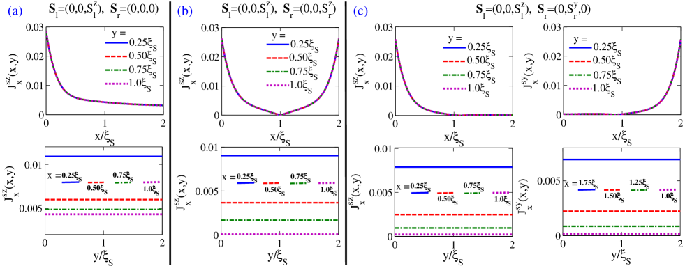
Figure 2: (Color online) Spatial profiles of the three spin current components, $J^{sx}_{x}(x,y)$, $J^{sy}_{x}(x,y)$, and $J^{sz}_{x}(x,y)$ in a $S$/$N$/$S$ junction with spin-active interfaces and no spin orbit interactions. Top row panels are against $x$ (positions along the junction length) at differing locations along $y=0.25\xi_{S},0.5\xi_{S},0.75\xi_{S},1.0\xi_{S}$ (see Fig. 1). By contrast, the bottom row panels are functions of $y$, plotted at four positions along the junction length $x=0.25\xi_{S},0.5\xi_{S},0.75\xi_{S},1.0\xi_{S}$. For the $N$ wire we have, $d_{N}=W_{N}=2.0\xi_{S}$, and the phase difference between the $S$ electrodes is fixed at $\varphi=\pi/2$. The spin moments of the spin-active interfaces are denoted by ${\bm{S}}_{lr}=(S^{x}_{lr},S^{y}_{lr},S^{z}_{lr})$ at the left($l$) and right($r$) interfaces. (a) The right interface is spin-inactive while the spin moment of left interface points along the $z$ direction, ${\bm{S}}_{l}=(0,0,\pm S^{z}_{l})$. In (b), the two interfaces are spin-active with parallel spin moments ${\bm{S}}_{lr}=(0,0,\pm{S}^{z}_{lr})$ while in (c), ${\bm{S}}_{l}=(0,0,\pm S^{z}_{l})$ and ${\bm{S}}_{r}=(0,\pm S^{y}_{r},0)$.

One of the most striking topics in the study of transport in junction systems involves spin currents. Since a decade ago, various features and behaviors of spin currents in hybrid structures have extensively been studied.Nikolic ; kato_1 ; hirsh_1 ; malsh_sns ; malsh_severin ; mishchenko_1 ; Sinova_1 ; gorini_3 ; gorini_1 ; Demidov The spin and charge currents are key quantities that reveal useful insights into the system transport characteristics. These physical quantities are also crucial to the application of nanoscale elements in superconducting spintronics devices.buzdin_rmp ; bergeret1 The vector charge (${\bm{J}}^{c}$) and spin (${\bm{J}}^{s\gamma}$) current densities can be calculated by the Keldysh block ($K$) when the system is in equilibrium:gorini_1 ; gorini_3

$${\bm{J}}^{c}({\bm{r}},\varphi)=J_{0}^{c}\bigg{|}\int_{-\infty}^{+\infty}d\varepsilon\text{Tr}\Big{\{}{\rho}_{3}\big{(}{G}({\bm{r}})[{\bm{\partial}},{G}({\bm{r}})]\big{)}^{K}\Big{\}}\bigg{|},$$ (30)

$${\bm{J}}^{s\gamma}({\bm{r}},\varphi)=J_{0}^{s}\bigg{|}\int_{-\infty}^{+\infty}d\varepsilon\text{Tr}\Big{\{}{\rho}_{3}\nu^{\gamma}\big{(}{G}({\bm{r}})[{\bm{\partial}},{G}({\bm{r}})]\big{)}^{K}\Big{\}}\bigg{|},$$ (31)

where $J_{0}^{c}=N_{0}eD/4$, $J_{0}^{s}=\hbar J_{0}^{c}/2e$, and $N_{0}$ is the number of states at the Fermi surface. The vector current densities provide local directions and amplitudes for the currents as a function of position. We designate $\gamma=x,y,z$ for the three components of spin current, e.g., ${\bm{J}}^{sx}$ represents the $x$ component of spin current. The integral of Eq. (30) over the $y$ direction, shown in Fig. 1, provides the total charge supercurrent flowing across the system.

In order to pinpoint the behavior of the spin-singlet and spin-triplet pairings inside the spin-orbit coupled $N$ wire, we exploit a spin-parametrization schemebuzdin_rmp ; bergeret1 ; alid_4 where the anomalous component of the Green’s function, Eq. (10), can be parameterized as follows:

$${\mathcal{F}}({\bm{r}},\varepsilon)=\mathbb{S}({\bm{r}},\varepsilon)+{\bm{\sigma}}\cdot{\bf T}({\bm{r}},\varepsilon)=$$

$$\sigma^{0}\mathbb{S}({\bm{r}},\varepsilon)+{\sigma}^{x}{{\text{T}}}_{x}({\bm{r}},\varepsilon)+{\sigma}^{y}{{\text{T}}}_{y}({\bm{r}},\varepsilon)+{\sigma}^{z}{{\text{T}}}_{z}({\bm{r}},\varepsilon).$$ (32)

In terms of this spin-parametrization, the quantities ${\mathbb{S}}$ and $T_{x,y}$ then correspond to the singlet and triplet components with $m=\pm 1$ total spin projection along the spin quantization axis, while $T_{z}$ represents the triplet component with $m=0$.bergeret1 ; buzdin_rmp ; spnactv_6 Here, the spin quantization axis is assumed fixed along the $z$ direction throughout the entire system. In a uniform ferromagnetic system, it has been demonstrated that the singlet and $m=0$ triplet component decay rapidly while the $m=\pm 1$ triplet components, if exist, can propagate over longer distances compared to the former correlations. By noting this aspect of triplet correlations, namely, the degree of their penetration (i.e. the distance that the correlations are nonzero) into a system, one may classify them as ‘short-range’ and ‘long-range’ correlations. Considering this classification, the $m=0$ triplet component in a uniform ferromagnet is short-ranged while the $m=\pm 1$ are long-ranged.bergeret1 ; buzdin_rmp Therefore, the parametrization scheme we utilize allows for explicit determination of the spatial profiles for the different superconducting pairings in intrinsically spin-orbit $S$/$N$/$S$ systems with spin-active interfaces and hence, their short-range and long-range natures.

III Results and discussions

For additional insight and comparison purposes, we first consider a $S$/$N$/$S$ junction with negligible SOIs and either one or two spin-active interfaces. We compute the spin currents, and discuss the singlet and triplet correlations in such systems. Next, we compute these same quantities after incorporating one of the Rashba or Dresselhaus ISOIs introduced above. As remarked earlier, Eq. (1) in the presence of ISOI terms leads to lengthy coupled partial differential equations. Although we have analytically derived the current densities [Eqs. (30) and (31)] for numerical implementation, they lead to cumbersome expressions that are not repeated here. In what follows, we normalize the quasiparticle energy $\varepsilon$ by the superconducting gap at zero temperature $\Delta_{0}=\Delta(\mathcal{T}=0)$, and all lengths by the superconducting coherence length $\xi_{S}$ which is defined as $\sqrt{\hbar\mathfrak{D}/\Delta_{0}}$. The barrier resistance at the $S$/$N$ interfaces is set to $\zeta=4$. This value of the barrier resistance warrants the validity of the low proximity limit i.e. $\mathcal{G}({\bm{r}},\varepsilon)\simeq 1$ and $\mathcal{F}({\bm{r}},\varepsilon)\ll 1$. We consider a fixed value for the spin moment amplitude of the spin-active interfaces, $|{\bm{S}}_{lr}|=G_{T}(\phi_{lr})^{-1}=15$, corresponding to realistic experimental situations.Sprungmann Here, $G_{T}$ is the barrier conductance and $\phi_{lr}$ represents the spin-dependent interfacial phase-shifts at the left and right interfaces.spnactv_21 ; spnactv_12 ; spnactv_1 We note that by considering other values for $|{\bm{S}}_{lr}|$, within reasonable experimental bounds, the influence on the results is negligible. In our actual computations, we have adopted natural units, so that $k_{B}=\hbar=1$. To find stable solutions to Eq. (1), and thus to obtain currents given by Eqs. (30) and (31), we have added a small imaginary part, $\delta\sim 0.01\Delta_{0}$, to the quasiparticles’ energy $\varepsilon\rightarrow\varepsilon+i\delta$. Physically, the additional imaginary part can be considered as a contribution from inelastic scatterings.alidoust_1 Due to this imaginary part, we have taken the modulus of quantities (denoted by the usual $|...|$). Also, for symmetry reasons we restrict the spatial profiles to the regions $0<x<d_{N}/2$ and $0<y<W_{N}/2$ in the figures presented throughout the paper.

III.1 $S$/$N$/$S$ junctions with spin active interfaces in the absence of SOC

Figure 2 displays the spatial profile of the spin current components in a $S$/$N$/$S$ junction containing spin-active interfaces and negligible SOIs. As seen in Fig. 1, the junction resides in the $xy$ plane so that the $S$/$N$ interfaces are located at $x=0,d_{N}$ and the vacuum borders in the $y$ direction are found at $y=0,W_{N}$. The junction width $W_{N}$ and length $d_{N}$ are set to a representative value of $2.0\xi_{S}$, without loss of generality. The top set of panels in Fig. 2 are functions of the $x$ coordinate at differing $y$, i.e., $0.25\xi_{S},0.5\xi_{S},0.75\xi_{S}$, and $1.0\xi_{S}$, while the bottom row of panels are functions of $y$ at fixed $x=0.25\xi_{S},0.5\xi_{S},0.75\xi_{S}$, and $1.0\xi_{S}$. In Fig. 2(a), the spin moment of the left interface is fixed along $z$, ${\bm{S}}_{l}=(0,0,\pm S^{z}_{l})$, while the right interface is spin-inactive, ${\bm{S}}_{r}=0$. Note that we have denoted vector ${\bm{S}}$ by three ‘positive’ scalar entries $S^{x},S^{y},S^{z}$, representing projection of the vector in the $x,y,z$ directions (in the Cartesian coordinate). Here, thus, $\pm$ signs indicate the orientation of that component which can be parallel (+) or antiparallel (-) to specific directions $x,y,z$. It can be seen that the only nonzero component of spin current is ${\bm{J}}^{sz}(x,y)$ due to ${\bm{S}}_{l}=(0,0,\pm S^{z}_{l})$. This component of spin current is maximum at the left $S$/$N$ interface, $x=0$, because of the abrupt spin-imbalance, and drops to a vanishingly small value near the right interface, $x=d_{N}$, which decays to zero over the much longer $d_{N}$ length scale. Moreover, the plot demonstrates a uniform distribution of spin current along $y$. We see that the curves at various $y$ locations overlap, consistent with the bottom panel of Fig. 2(a), where the spin current is constant for a given $x$.

As described above and seen in Fig. 2, the results for the two-dimensional $S$/$N$/$S$ junction in the absence of ISOIs reduces it to an effectively one-dimensional problem. Hence, to gain more insight, we derive analytical expressions for the charge and spin current densities in a simple structure, namely a one-dimensional $S$/$N$/$S$ junction with a single spin-active interface. To this end, we first derive solutions to the components of the Green’s function, Eq. (II), i.e. $f_{\pm}({\bm{r}},\pm\varepsilon)$, $[f_{\pm}({\bm{r}},\pm\varepsilon)]^{*}$, $f_{\upuparrows,\downdownarrows}({\bm{r}},\pm\varepsilon)$, and $[f_{\upuparrows,\downdownarrows}({\bm{r}},\pm\varepsilon)]^{*}$ in a one-dimensional $S$/$N$/$S$ junction where ${\bm{S}}_{l}=(0,0,\pm S^{z}_{l})$ and ${\bm{S}}_{r}=0$. If we define a normalized coordinate $\tilde{x}=x/d_{N}$, we end up with the following expression for $f_{-}(x,-\varepsilon)$ (similar expressions arise for the other components):

$$f_{-}(x,-\varepsilon)=s^{*}(\varepsilon)\times$$

$$e^{-i\varphi/2}\frac{\zeta\lambda[\cosh\lambda\tilde{x}+e^{i\varphi}\cosh\lambda(1-\tilde{x})]-iS_{l}^{z}\sinh\lambda\tilde{x}}{\zeta\lambda[\zeta\lambda\sinh\lambda-iS_{l}^{z}\cosh\lambda]}.$$

To simplify the solutions, we denote $2i\varepsilon/\varepsilon_{T}=\lambda$ (in which $\varepsilon_{T}$ is the Thouless energy) and assume $\theta_{lr}=\pm\varphi/2$. By substituting the obtained solutions into Eq. (30) we arrive at the following expression for the charge current:

$$J_{x}^{c}(x,\varphi)=J_{0}^{c}\int_{-\infty}^{+\infty}d\varepsilon 2i\lambda\tanh(\frac{\varepsilon k_{B}T}{2})\frac{{\cal N}^{c}}{{\cal D}^{c}}\sin\varphi,$$ (33)

$${\cal N}^{c}=$$

$${[s^{*}(-\varepsilon)]}^{2}\sin\lambda\Big{\{}{S^{z}_{l}}^{2}-\zeta^{2}\lambda^{2}+({S^{z}_{l}}^{2}+\zeta^{2}\lambda^{2})\cosh 2\lambda\Big{\}}$$

$$+{[s^{*}(\varepsilon)]}^{2}\sinh\lambda\Big{\{}{S^{z}_{l}}^{2}+\zeta^{2}\lambda^{2}+({S^{z}_{l}}^{2}-\zeta^{2}\lambda^{2})\cos 2\lambda\Big{\}},$$

$${\cal D}^{c}=$$

$$\Big{\{}{S^{z}_{l}}^{2}\cos^{2}\lambda+\zeta^{2}\lambda^{2}\sin^{2}\lambda\Big{\}}\Big{\{}{S^{z}_{l}}^{2}\cosh^{2}\lambda+\zeta^{2}\lambda^{2}\sinh^{2}\lambda\Big{\}}.$$

It is immediately evident that the charge current has the usual $\sin\varphi$ odd-functionality in the superconducting phase difference. The same procedure is followed to derive analytical expressions for the spin current components using Eq. (31). Since ${\bm{S}}_{l}=(0,0,\pm S^{z}_{l})$, we find $J^{sx}_{x}(x,\varphi)=J^{sy}_{x}(x,\varphi)\equiv 0$ and $J^{sz}_{x}(x,\varphi)\neq 0$. Unfortunately, even by means of the simplifying approximations made to the equations thus far, we arrive at a rather lengthy expression for the $z$ component of the spin current, $J^{sz}_{x}(x,\varphi)$.ma_kh_njp Nevertheless, if we restrict our attention to the edge of the wire, $x=0$, this spin current component reduces to the following:

$$J^{sz}_{x}(\varphi) = J_{0}^{s}\int_{-\infty}^{+\infty}d\varepsilon\frac{4iS^{z}_{l}}{\zeta}\tanh(\frac{\varepsilon k_{B}T}{2})\Big{\{}\frac{{\cal N}_{1}^{sz}}{{\cal D}_{1}^{sz}}+\frac{{\cal N}_{2}^{sz}}{{\cal D}_{2}^{sz}}\Big{\}},$$ (34)

$${\cal N}_{1}^{sz} = [s^{*}(-\varepsilon)]^{2}\Big{\{}2{S^{z}_{l}}^{2}[1+\cos\lambda\cos\varphi]+\zeta^{2}\lambda^{2}[\cos 4\lambda-$$

$$6\cos\lambda\cos\varphi-3]+2[{S^{z}_{l}}^{2}+\zeta^{2}\lambda^{2}+({S^{z}_{l}}^{2}+3\zeta^{2}\lambda^{2})$$

$$\cos\lambda\cos\varphi]\cos 2\lambda\Big{\}},$$

$${\cal N}_{2}^{sz} = [s^{*}(\varepsilon)]^{2}\Big{\{}3[{S^{z}_{l}}^{2}+\zeta^{2}\lambda^{2}]\cosh\lambda\cos\varphi+$$

$$4{S^{z}_{l}}^{2}\cosh^{2}\lambda+({S^{z}_{l}}^{2}-3\zeta^{2}\lambda^{2})\cosh 3\lambda\cos\varphi$$

$$-4\zeta^{2}\lambda^{2}[2+\cosh 2\lambda]\sinh^{2}\lambda\Big{\}},$$

$${\cal D}_{1}^{sz} = \Big{\{}{S^{z}_{l}}^{2}+\zeta^{2}\lambda^{2}+[{S^{z}_{l}}^{2}-\zeta^{2}\lambda^{2}]\cos 2\lambda\Big{\}}^{2},$$

$${\cal D}_{2}^{sz} = \Big{\{}{S^{z}_{l}}^{2}-\zeta^{2}\lambda^{2}+[{S^{z}_{l}}^{2}+\zeta^{2}\lambda^{2}]\cosh 2\lambda\Big{\}}^{2}.$$

The $z$ component of spin current, $J^{sz}_{x}$, is evidently an even-function of $\varphi$, namely $\cos\varphi$, although it involves some complicated prefactors.ma_kh_njp This finding is consistent with Ref. alidoust_1, . Note that when the other components of spin current, ${\bm{J}}^{s\gamma}$, are present, the even-functionality in $\varphi$ holds, even in the presence of ISOIs. This effect is discussed further below.

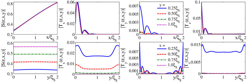
Figure 3: (Color online) The spatial behaviors of the singlet $\mathbb{S}(\varepsilon,x,y)$ and triplet ${\bf T}(\varepsilon,x,y)$ correlations inside a Rashba $S$/$N$/$S$ system with ${\bf S}_{l}=(0,0,\pm S^{z}_{l})$ and ${\bf S}_{r}=0$. The quasiparticles’ energy is set at $\varepsilon=0.1\Delta_{0}$, $d_{N}=W_{N}=2.0\xi_{S}$, and $\varphi=\pi/2$. The top panels display the various pair correlations vs $x$ at $y=0.25\xi_{S}$, $0.5\xi_{S}$, $0.75\xi_{S}$, and $1.0\xi_{S}$, whereas the bottom panels exhibit the same quantities as a function of $y$ at $x=0.25\xi_{S}$, $0.5\xi_{S}$, $0.75\xi_{S}$, and $1.0\xi_{S}$.

In Fig. 2(b), the right interface is now spin-active (at $x=d_{N}$). The spin moment direction of the spin-active interface at $x=0$ is intact while ${\bm{S}}_{r}=(0,0,\pm S^{z}_{r})$. As seen in the bottom panel, ${\bm{J}}^{sz}(x,y)$ is still the only nonzero spin current component, which is constant in the $y$ direction. The right spin-active interface causes an increase in ${\bm{J}}^{sz}(x,y)$ at $x=d_{N}$ due to a spin-imbalance effect. In Fig. 2(c), the spin moment of the interface at $x=d_{N}$ is oriented along the $y$ direction, i.e., ${\bm{S}}_{r}=(0,\pm S^{y}_{r},0)$. We see that ${\bm{J}}^{sy}(x,y)$ and ${\bm{J}}^{sz}(x,y)$ are both nonzero since ${\bm{S}}_{l}$ and ${\bm{S}}_{r}$ are orthogonal. The spin current vanishes at the middle of the junction ($x=d_{N}/2$) and apparently the behavior of the components become interchanged at this location. From the bottom row of panels in Fig. 2, we see that the spin-active interfaces with various spin moment orientations would lead to uniformly distributed spin currents along the junction width in the $y$ direction. In other words, the spin-active interfaces alone are unable to induce any spin accumulation at the vacuum borders of the $N$ wire.Nikolic ; kato_1 ; hirsh_1 ; malsh_severin ; mishchenko_1 ; Sinova_1 ; gorini_3 ; gorini_1 The triplet correlations in superconducting hybrids with spin-active interfaces have extensively been studied. spnactv_16 ; spnactv_12 ; spnactv_1 In $S$/$N$/$S$ systems with a single spin-active interface, no equal-spin pairing can arise (since a single quantization axis exists throughout the whole system), although opposite-spin triplets, $\text{T}_{z}(x,y)$, can be induced. Figure 2(a), where only $J_{x}^{sz}$ is nonvanishing, confirms this phenomenon.

III.2 Intrinsic spin orbit coupled $S$/$N$/$S$ junctions with a single spin active interface: Singlet and triplet correlations

Now we incorporate ISOIs in the $S$/$N$/$S$ junction with one spin-active interface at $x=0$ (see Fig. 1). Figure 3 exhibits first spatial profiles of the singlet ($\mathbb{S}(\varepsilon,x,y)$) and triplet ($\text{T}_{x,y,z}(\varepsilon,x,y)$) correlations. Here we set ${\bm{S}}_{l}=(0,0,\pm S^{z}_{l})$, ${\bm{S}}_{r}=0$, and assume that the ISOI is of the Rashba form, i.e., $\alpha\neq 0$, and $\beta=0$ (we later discuss the results of a Dresselhaus SOC). We choose $\alpha=2.0\xi_{S}^{-1}$bergeret_so as a representative value and emphasize that this specific choice has no influence on the generality of our findings. In the low proximity limit, quasiparticles with low energies ($\varepsilon\ll 1$) tend to have the main contributions to the pair correlations. Accordingly, we therefore choose a representative value for the quasiparticles’ energy equal to $\varepsilon=0.1\Delta_{0}$. The other parameters are kept unchanged. As clearly seen, the combination of an ISOI and spin moment of only one spin-active interface results in three nonzero components of the triplet correlations, which is in contrast to the case with zero ISOI shown in Fig. 2. This phenomena directly follows from the fact that the quasiparticle spin is tied to its momentum in the presence of an ISOI.bergeret_so The singlet $|\mathbb{S}(\varepsilon,x,y_{0})|$ is minimum at $x=0$ and increases monotonically towards $x=d_{N}$ at every point along the junction width $y_{0}=0.25\xi_{S},0.5\xi_{S},0.75\xi_{S}$, and $1.0\xi_{S}$. This behavior can be understood by noting the combination of interface spin moment and ISOIs at $x=0$ abruptly converts the singlet correlations into triplet correlations. This picture is however reversed at $x=d_{N}$ where an ingredient to the singlet-triplet conversion is lacking, i.e., ${\bm{S}}_{r}=0$ at $x=d_{N}$. Examining the spatial map of the triplet correlations in Fig. 3, we find that the triplet correlations behave oppositely to the singlets. The triplet correlations $\text{T}_{x,y,z}(\varepsilon,x,y_{0})$ are maximum near $x=0$, where the $S$/$N$ interface is spin-active. Here, as remarked above, the combination of interface spin moment and ISOIs effectively converts the singlet superconducting correlations into the triplet ones at $x=0$. The triplet correlations decline as a function of $x$, and eventually convert into the singlets at $x=d_{N}$ (at the spin-inactive interface). The triplet correlations, $\text{T}_{x,y}$, have nonzero spin-projections along the spin-quantization axis ($m=\pm 1$) while $m=0$ for the $\text{T}_{z}$ component. It is evident that $\text{T}_{z}$ is drastically suppressed when moving away from the spin-active $S$/$N$ interface at $x=0$ (a consequence of the so-called short-range behavior of $\text{T}_{z}$). The spin-1 quantities, $\text{T}_{x,y}$, on the other hand, remain nonzero over greater distances (the so-called long-range behavior). The actual distances that the triplet correlations can propagate over them before fully vanishing in a system depends on the system parameters such as temperature, degree of the interface opacity $\zeta$, strength of the interface spin-activity and the magnitude of SOCs present in the system. Nonetheless, a direct comparison of penetration depth between the triplet correlations with zero total spin $\text{T}_{z}$ and nonzero total spin i.e. $\text{T}_{x,y}$ clearly reveals that $\text{T}_{z}$ is the short-ranged triplet component while $\text{T}_{x,y}$ are long-ranged in the ISO coupled $S$/$N$/$S$ junction with one spin-active interface. We note that this conclusion generally holds, independent of the representative values chosen. The bottom set of panels in Fig. 3 illustrates the superconducting correlations $|\mathbb{S}(\varepsilon,x_{0},y)|$, and $|\text{T}_{x,y,z}(\varepsilon,x_{0},y)|$ as functions of $y$-position along the junction width where $x_{0}=0.25\xi_{S},0.5\xi_{S},0.75\xi_{S}$, and $1.0\xi_{S}$. The spatial distribution of the singlet correlations along $y$ are unaffected by the coupling of the ISOIs and interface spin moment at $x=0$. The singlets, $|\mathbb{S}(\varepsilon,x_{0},y)|$, are constant along $y$, implying a uniform distribution along the junction width. This however differs considerably from the spatial behavior of the triplet correlations: The three triplet components $|\text{T}_{x,y,z}(\varepsilon,x_{0},y)|$ demonstrate appreciable accumulation at the transverse vacuum boundaries of the $N$ wire (at $y=0$, and $y=W_{N}$). Also, the results reveal that the maximum singlet-triplet conversions occur at the corners of the $N$ strip near the spin-active interface (near $x=0$, $y=0$ and $x=0$, $y=W_{N}$).ma_kh_njp Further investigations have demonstrated that the maximum singlet-triplet conversion in such systems generally takes place at the corners of the $N$ wire near any spin-active interfaces.ma_kh_njp We note that this finding is generic, robust, and independent of either interface spin moment direction or the actual type of ISOI considered. Similar spatial profiles appear when $\alpha=0$, and $\beta\neq 0$, or equivalently when a Dresselhaus SOI is considered. Our numerical investigations have found that the corresponding Dresselhaus SOI results can be straightforwardly obtained by making the following replacements in Fig. 3: $|\mathbb{S}^{\text{R}}(\varepsilon,x,y)|=|\mathbb{S}^{\text{D}}(\varepsilon,x,y)|$, $|{\text{T}}^{\text{R}}_{z}(\varepsilon,x,y)|=|{\text{T}}^{\text{D}}_{z}(\varepsilon,x,y)|$, $|{\text{T}}^{\text{R}}_{x}(\varepsilon,x,y)|=|{\text{T}}^{\text{D}}_{y}(\varepsilon,x,y)|$, and $|{\text{T}}^{\text{R}}_{y}(\varepsilon,x,y)|=|{\text{T}}^{\text{D}}_{x}(\varepsilon,x,y)|$. The symmetries can be easily understood by considering the symmetries of the spin-dependent fields in Eq. (29), resulting in Rashba and Dresselhaus SOIs.bergeret_so The spin current components also show similar symmetries and we shall discuss them in detail at the end of this section.

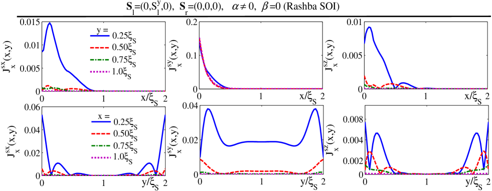
Figure 4: (Color online) The spin current components, $J^{sx}_{x}(x,y)$, $J^{sy}_{x}(x,y)$, $J^{sz}_{x}(x,y)$ in a Rashba ($\alpha\neq 0,\beta=0$) $S$/$N$/$S$ junction with one spin-active interface (at $x=0$). The interface spin moment is oriented along the $y$ direction ${\bf S}_{l}=(0,\pm S^{y}_{l},0)$ and ${\bf S}_{r}=0$ (see Fig. 1). The top panels show the spin currents vs $x$ at $y=0.25\xi_{S},0.5\xi_{S},0.75\xi_{S}$, and $1.0\xi_{S}$. The bottom panels exhibit the same quantities as a function of $y$ at $x=0.25\xi_{S},0.5\xi_{S},0.75\xi_{S}$, and $1.0\xi_{S}$. The superconducting phase difference is set at $\varphi=\pi/2$, and $d_{N}=W_{N}=2.0\xi_{S}$.

III.3 Intrinsic spin orbit coupled $S$/$N$/$S$ junctions with a single spin active interface: Spin currents

Figure 4 exhibits the corresponding spatial profiles of the spin current components, given by Eq. (31) for a Rashba $S$/$N$/$S$ junction with one spin-active interface. We assume that the left interface at $x=0$ is spin-active (see Fig. 1), and its spin moment is oriented along the $y$ direction, namely, ${\bm{S}}_{l}=(0,\pm S^{y}_{l},0)$ (and thus ${\bm{S}}_{r}=0$). To be specific, we first present the results of a Rashba ($\alpha\neq 0,\beta=0$) $S$/$N$/$S$ system in our plots and then later expand our discussion to differing orientations of ${\bm{S}}_{l}$ in the presence of either Rashba or Dresselhaus SOIs. The top row of panels in Fig. 4 display the three components of spin current density $J^{s\gamma}_{x}(x,y_{0})$ flowing along $x$ at $y_{0}=0.25\xi_{S},0.5\xi_{S},0.75\xi_{S}$, and $1.0\xi_{S}$. The spatial variations of the $x$ component provides the clearest and most useful information on the spin current behavior in such systems. Therefore, we only present the $x$ components in Fig. 4, while later discussing the vector spin current densities when presenting symmetries among the spin current components. The spin current density components vanish within $x>d_{N}/2$ while they are largest near the spin-active interface at $x=0$. This behavior is consistent with the associated triplet correlations investigated in the top row of panels in Fig. 3. The spin currents are zero at $x=d_{N}$, where the $S$/$N$ interface is spin-inactive. This finding is also consistent with previous theoretical works where the spin currents were found to vanish at $S$/$N$ interfaces,malsh_sns and thus there were zero spin currents throughout the entire ISO coupled $S$/$N$/$S$ hybrids. Since the $S$/$N$/$S$ system considered here is in an equilibrium state, the time derivative of the spin density is equal to zero. gorini_1 Therefore, because the singlet superconducting electrodes considered throughout the paper do not support spin currents, the divergence of the spin current at a $S$/$N$ interface is zero if the spin moment of the spin-active interface is zero (spin-inactive interfaces). This fact is clearly seen in Figs. 2(a) and 4 where the right $S$/$N$ interface is spin-inactive. The bottom panels display the same components except now as a function of $y$ along the junction width $J^{s\gamma}_{x}(x_{0},y)$ at $x_{0}=0.25\xi_{S},0.5\xi_{S},0.75\xi_{S}$, and $1.0\xi_{S}$. Most notably, the plots reveal a nonuniform distribution of spin current densities along the junction width. From the plots, it is apparent that the spin current densities peak near the transverse vacuum boundaries of the $N$ wire at $y=0$, and $y=W_{N}$. Considering the top and bottom panels together, we conclude that the spin currents are maximally accumulated at the edges of the $N$ wire near the spin-active interface and approximately confined within $x<d_{N}/2$. This in turn implies that the corners of the $N$ wire near the spin-active interfaces possess the maximum of spin current densities.ma_kh_njp The edge accumulation of spin current densities are reminiscent of those previously found in nonsuperconducting mesoscale junctions with ISOIs. Murakami_1 ; hirsh_1 ; kato_1 ; Sinova_1 ; mishchenko_1 ; chazalviel ; Nikolic We emphasize that the previous works relied critically on externally applied magnetic and electric fieldsMurakami_1 ; hirsh_1 ; kato_1 ; Sinova_1 ; mishchenko_1 ; chazalviel ; Nikolic ; malsh_sns ; malsh_severin which can complicate the theoretical and experimental situations. In contrast, our findings provide an alternate, simple platform which relies merely on the intrinsic properties of the system and is devoid of any externally imposed conditions. Our numerical approach allows us to determine the precise nature of the spin and charge currents when varying the superconducting phase difference, $\varphi$. The spatial maps of charge supercurrent density (not shown) are constant vs position within the $N$ wire, reflecting the charge conservation law. We have found that the charge supercurrent is governed by a sinusoidal-like current phase relation, while the spin currents, on the contrary, are even-functionsalidoust_1 , i.e., ${\bm{J}}^{s\gamma}(\varphi+2\pi)={\bm{J}}^{s\gamma}(-\varphi)$. The behavior of charge supercurrent in the low proximity limit considered here can differ from the ballistic regime where anomalous supercurrent-phase relations were found Konschelle ; yokoyama ; reynoso_1 . These findings offer an appealing experimental platform to examine pure edge spin currents, not accompanied by charge currents, solely by modulating $\varphi$ without imposing an external electromagnetic field on the system.

A spin-active $S$/$N$ interface can be ordinarily fabricated by coating a superconductor with a spin-active layer. spnactv_14 ; spnactv_8 ; spnactv_15 ; spnactv_20 ; spnactv_1 The signatures of triplet pairings can be experimentally probed by means of tunneling experiments and scanning tunneling microscopy/spectroscopy (STM/STS) techniquesDOS_measur_th , which rely on zero-energy peaks in the proximity-induced density of statesspnactv_14 ; DOS_1_ex ; DOS_2_ex . Technological progress allows for measuring high resolution spatially and energy resolved density of states on a two-dimensional surface.DOS_1_ex ; DOS_2_ex Therefore, the accumulation of triplet correlations at the boundaries or corners of an $N$ wire, and also their long-range signatures predicted here, may be realized in tunneling experiments. Indeed, one such possibility is shown in the schematic of Fig. 1, where the STM tip can traverse the surface and effectively measure the local density of states of the entire $N$ layer residing in the $xy$ plane, producing a spatially-resolved and energy-resolved density of statesDOS_1_ex ; DOS_2_ex . Based on our findings described thus far, one can expect significant modifications to the local density of states as the STM tip moves toward the edges of the $N$ layer and probes the signatures of triplet pairings, which manifest themselves in zero-energy peaks of the local density of states.

Magnetic moment ${\bm{S}}_{l}$=$(S^{x}_{l},S^{y}_{l},S^{z}_{l})$ ${\bm{S}}_{r}$=$(0,0,0)$	${\bm{S}}_{l}$=$(\pm S^{x}_{l},0,0)$			${\bm{S}}_{l}$=$(0,\pm S^{y}_{l},0)$			${\bm{S}}_{l}$=$(0,0,\pm S^{z}_{l})$
Rashba SOI	${\bm{J}}^{sx}$	${\bm{J}}^{sy}$	${\bm{J}}^{sz}$	${\bm{J}}^{sx}$	${\bm{J}}^{sy}$	${\bm{J}}^{sz}$	${\bm{J}}^{sx}$	${\bm{J}}^{sy}$	${\bm{J}}^{sz}$
Magnetic moment ${\bm{S}}_{l}$=$(S^{x}_{l},S^{y}_{l},S^{z}_{l})$ ${\bm{S}}_{r}$=$(0,0,0)$	${\bm{S}}_{l}$=$(0,\pm S^{y}_{l},0)$			${\bm{S}}_{l}$=$(\pm S^{x}_{l},0,0)$			${\bm{S}}_{l}$=$(0,0,\pm S^{z}_{l})$
Dresselhaus SOI	${\bm{J}}^{sy}$	${\bm{J}}^{sx}$	${\bm{J}}^{sz}$	${\bm{J}}^{sy}$	${\bm{J}}^{sx}$	${\bm{J}}^{sz}$	${\bm{J}}^{sy}$	${\bm{J}}^{sx}$	${\bm{J}}^{sz}$

Table 1: Symmetries of the spin current components, ${\bm{J}}^{s\gamma}(x,y)$, in an intrinsic spin-orbit coupled $S$/$N$/$S$ junction with one spin-active interface depicted in Fig. 1. The spin moments of the left and right interfaces are denoted by ${\bm{S}}_{lr}$ and the spin-orbit coupling is set to be either purely of the Rashba ($\alpha\neq 0$, $\beta=0$) or Dresselhaus ($\beta\neq 0$, $\alpha=0$) type. To have succinct notation, the $(x,y)$-functionality of the spin current components is omitted in the table. The spin current components in similar columns have identical modulus behaviors.

Spin accumulation is a distinctive trademark of the spin-Hall effect.malsh_sns Therefore, the accumulation of spin current densities at the edges of the sample, as described in this paper, may be directly measurable through optical experiments such as Kerr rotation microscopykato_1 . In this scenario spatial maps of the spin polarizations in the entire $N$ wire can be conveniently imaged. A multiterminal device can also be alternatively employed to observe the signatures of spin currents edge accumulation Nikolic ; mishchenko_1 ; latrl . When lateral leads are attached near the transverse vacuum edges of a two-dimensional $S$/$N$/$S$ junction (vacuum boundaries at $y=0$, and $y=W_{N}$ in Fig. 1), the accumulated spin densities at the transverse edges of the $N$ wire can result in spin current injection into the lateral leads, which in turn may induce a voltage drop. Nikolic ; mishchenko_1 ; latrl

Finally, we discuss the symmetries present among the components of spin current density by varying the spin moment orientation of a spin-active interface, shown in Fig. 1, in a Rashba or Dresselhaus $S$/$N$/$S$ hybrid. In order to systematically obtain and compare results, we first consider a Rashba SOI ($\alpha\neq 0,\beta=0$) and rotate ${\bm{S}}_{l}$ while ${\bm{S}}_{r}=0$. Thereafter, we iterate the same procedure when the SOI is purely Dresselhaus ($\alpha=0,\beta\neq 0$). Table 1 summarizes the symmetries among the components of spin current found through extensive numerical investigations. In the table, vector currents are presented, i.e., ${\bm{J}}^{s\gamma}(x,y)=(J_{x}^{s\gamma},J_{y}^{s\gamma}$, and $J_{z}^{s\gamma})$. The spin current components with identical spatial maps reside in similar columns. For example, ${\bm{J}}^{sx}(x,y)$ in the first row and column is identical to ${\bm{J}}^{sy}(x,y)$ in the second row and first column. In the top row, labeled “Rashba SOI”, we consider Rashba SOC and rotate the spin moment of the left interface ${\bm{S}}_{l}$. In the bottom row (labeled “Dresselhaus SOI”), however, Dresselhaus SOI is considered and the spin moment rotations, the same as Rashba case, are iterated. As seen, when the moment of the spin-active interface points along the $z$ direction ${\bm{S}}_{l}=(0,0,\pm S^{z}_{l})$, ${\bm{J}^{sz}}$ shows identical behaviors for either Rashba or Dresselhaus SOIs. However, ${\bm{J}^{sx}}$ (and ${\bm{J}^{sy}}$) in the presence of Rashba SOI is identical to ${\bm{J}^{sy}}$ (and ${\bm{J}^{sx}}$) in the presence of Dresselhaus SOI. This scenario changes when the moment of the spin-active interface points along the $x$ or $y$ directions. Similar symmetries to the previous case, i.e. ${\bm{S}}_{l}=(0,0,\pm S^{z}_{l})$, are available, provided that we transform ${\bm{S}}_{l}=(\pm S^{x}_{l},0,0)$ to ${\bm{S}}_{l}=(0,\pm S^{y}_{l},0)$, and vice a versa, when considering Rashba or Dresselhaus SOIs. For example, ${\bm{J}^{sz}}$ in the presence of Rashba SOI and ${\bm{S}}_{l}=(\pm S^{x}_{l},0,0)$ is identical to ${\bm{J}^{sz}}$ in the presence of Dresselhaus SOI, provided that ${\bm{S}}_{l}=(0,\pm S^{y}_{l},0)$. Under the same conditions, ${\bm{J}^{sx}}$ (and ${\bm{J}^{sy}}$) in the presence of Rashba SOI is identical to ${\bm{J}^{sy}}$ (and ${\bm{J}^{sx}}$) in the presence of Dresselhaus SOI. The contents of Table 1 can be utilized to deduce the spin current densities in the presence of Rashba (Dresselhaus) SOI solely by using the results of a Dresselhaus (Rashba) SOI, without any additional calculations. Similar transformations can take place based on other orientations of ${\bm{S}}_{l}$. Thus for example, this prescription can be used to obtain the spatial maps of spin current densities in a Dresselhaus $S$/$N$/$S$ junction with ${\bm{S}}_{l}=(\pm S^{x}_{l},0,0)$ and ${\bm{S}}_{r}=0$ using the data from the plots presented in Fig. 4.

IV Conclusions

In conclusion, finite-sized two-dimensional intrinsic spin-orbit coupled $S$/$N$/$S$ junctions with one spin-active interface in the diffusive regime are theoretically studied using a quasiclassical approach together with spin-dependent fields obeying SU(2) gauge symmetries. We have computed the singlet and triplet correlations, and the associated spin currents in a $S$/$N$/$S$ system where the interface spin moment can take arbitrary orientations. Using spatial maps of the singlet and triplet pair correlations within the two-dimensional $N$ wire, we demonstrate that the combination of one spin-active interface and an intrinsic spin-orbit interaction (ISOI) effectively converts singlet pairs into long-range triplet ones. Interestingly, the spatial profiles illustrate that the proximity-induced triplet correlations are nonuniformly distributed and accumulate at the borders of the $N$ wire nearest the spin-active interface. By contrast, the spatial amplitude of the singlet correlations is uniform within the spin-orbit coupled $N$ wire. The results suggest that the maximum singlet-triplet conversion takes place at the corners of the $N$ wire nearest the spin-active interface. The spatial profiles of the associated spin current densities also demonstrate that the three components of spin currents accumulate the most at the edges of the $N$ wire. Subsequently, the corners of the $N$ wire near the spin-active interface host maximum density of spin currents.ma_kh_njp These results are robust and independent of either the interface spin moment orientation or the actual type of ISOI. (We note that rich edge phenomena were theoretically found in finite-size two-dimensional intrinsically spin orbit coupled $S$/$F$/$S$ junctions in Ref. ma_kh_njp, ). We also determine the behavior of spin and charge currents by varying the macroscopic phase difference between the $S$ banks, $\varphi$. The charge supercurrent is governed by the usual odd-functionality in $\varphi$, while the spin currents are even-functions of $\varphi$, i.e. $J^{s}(\varphi+2\pi)=J^{s}(-\varphi)$.alidoust_1 Hence by properly calibrating $\varphi$, it is possible to have pure edge spin currents without driving charge supercurrents. We then described experimentally relevant signatures and potential experiments aimed at realizing the edge phenomena predicted here. Our work therefore offers a simple structure consisting of a finite-sized intrinsic spin-orbit coupled $S$/$N$/$S$ junction with one spin-active interface to generate various edge phenomena, such as singlet-triplet conversions, long-range proximity effects, and spin currents in the absence of externally imposed fields.

Appendix A Pauli Matrices

In Sec. II we introduced the Pauli matrices in the spin space and denoted them by ${\bm{\sigma}}=\big{(}\sigma^{x},\sigma^{y},\sigma^{z}\big{)}$, ${\bm{\tau}}=\big{(}\tau^{x},\tau^{y},\tau^{z}\big{)}$, and ${\bm{\nu}}=\big{(}\nu^{x},\nu^{y},\nu^{z}\big{)}$.

$$\sigma^{x}=\begin{pmatrix}0&1\\ 1&0\\ \end{pmatrix},\;\sigma^{y}=\begin{pmatrix}0&-i\\ i&0\\ \end{pmatrix},\;\sigma^{z}=\begin{pmatrix}1&0\\ 0&-1\\ \end{pmatrix},\;\sigma^{0}=\begin{pmatrix}1&0\\ 0&1\\ \end{pmatrix}.$$

We also introduced the $4\times 4$ matrices ${\bm{\rho}}=({\rho}_{1},{\rho}_{2},{\rho}_{3})$:

$${\rho}_{1}=\begin{pmatrix}0&\sigma^{x}\\ \sigma^{x}&0\\ \end{pmatrix},\;{\rho}_{2}=\begin{pmatrix}0&-i\sigma^{x}\\ i\sigma^{x}&0\\ \end{pmatrix},\;{\rho}_{3}=\begin{pmatrix}\sigma^{0}&0\\ 0&-\sigma^{0}\\ \end{pmatrix}.$$

Following Ref. alidoust_1, , we define $\tau^{\gamma}$, $\nu^{\gamma}$, and $\rho_{0}$ as follows;

$$\tau^{\gamma}=\begin{pmatrix}\sigma^{\gamma}&0\\ 0&\sigma^{\gamma}\\ \end{pmatrix},\;\nu^{\gamma}=\begin{pmatrix}\sigma^{\gamma}&0\\ 0&\sigma^{\gamma\ast}\\ \end{pmatrix},\;\rho_{0}=\begin{pmatrix}\sigma^{0}&0\\ 0&\sigma^{0}\\ \end{pmatrix},$$

to unify our notation throughout the paper $\gamma$ stands for $x,y,z$.

References

- (1) J.M. Kikkawa, and D.D. Awschalom, Nature 397, 139 (1999); D.D. Awschalom, and J.M. Kikkawa, Phys. Today 52(6), 33 (1999).
- (2) S.A. Wolf, D.D. Awschalom, R.A. Buhrman, J.M. Daughton, S. von Moln r, M.L. Roukes, A.Y. Chtchelkanova, D.M. Treger, Science 294, 1488 (2001).
- (3) D. Stepanenko and N.E. Bonesteel, Phys. Rev. Lett. 93, 140501 (2004).
- (4) H.A. Engel, E.I. Rashba, and B.I. Halperin, Handbook of Magnetism and Andvanced Magnetic Materials, edited by H. Kronmuller and s. Parkin (Wiley, Chichester, UK, 2007).
- (5) J. Wunderlich, B. Park, A.C. Irvine, L.P. Zarbo, E. Rozkotova, P. Nemec, V. Novak, J. Sinova, and T. Jungwirth, Science 330, 1801 (2010).
- (6) I.M. Miron, G. Gaudin, S. Auffret, B. Rodmacq, A. Schuhl, S. Pizzini, J. Vogel, and P. Gambardella, Nat. Mat. 9, 230 234 (2010).
- (7) S. Murakami, N. Nagaosa, S. Zhang, Science 301, 1348 (2003).
- (8) N. Nagaosa, J. Sinova, S. Onoda, A.H. MacDonald, and N.P. Ong, Rev. Mod. Phys. , 82, 1539 (2010).
- (9) R. Winkler, Spin-orbit coupling effects in two-dimensional electron and hole systems, Springer-Verlag, 2003; R. Winkler, H. Noh, E. Tutuc, and M. Shayegan, Phys. Rev. B 65, 155303 (2002).
- (10) D. Awschalom, N. Samarth, and D. Loss, Semiconductor spintronics and quantum computation, Springer, New York, 2002.
- (11) S.I. Erlingsson, J. Schliemann, and D. Loss, Phys. Rev. B 71, 035319 (2005).
- (12) Y. Asano, Y. Tanaka, M. Sigrist, and S. Kashiwaya, Phys. Rev. B67, 184505 (2003).
- (13) G. Dresselhaus, Phys. Rev. 100, 580 (1955).
- (14) G.A. Prinz, Science 282, 1660 (1998).
- (15) V.E. Demidov, S. Urazhdin, A.B. Rinkevich, G. Reiss, and S.O. Demokritov, Appl. Phys. Lett., 104, 152402 (2014).
- (16) S. Murakami, N. Nagaosa, and S.-C. Zhang, Science 301, 1348 (2003).
- (17) J. Sinova, D. Culcer, Q. Niu, N.A. Sinitsyn, T. Jungwirth, and A.H. MacDonald, Phys. Rev. Lett. 92, 126603 (2004).
- (18) J.N. Chazalviel, Phys. Rev. B 11, 3918 (1975).
- (19) M.I. Dyakonov and V.I. Perel, Phys. Lett. 35A, 459 (1971); J.E. Hirsh, Phys. Rev. Lett. 83, 1834 (1999).
- (20) Y.K. Kato, R.C. Myers, A.C. Gossard, and D.D. Awschalom, Science 306, 1910 (2004); J. Wunderlich, B. Kastner, J. Sinova, and T. Jungwirth, Phys. Rev. Lett. 94, 047204 (2005).
- (21) E.G. Mishchenko, A.V. Shytov, and B.I. Halperin, Phys. Rev. Lett. 93, 226602 (2004).
- (22) B.K. Nikolic, S. Souma, L.P. Zarbo, and J. Sinova, Phys. Rev. Lett. 95, 046601 (2005).
- (23) A.G. Malshukov, S. Sadjina, and A. Brataas, Phys. Rev. B81, 060502(R) (2010).
- (24) M.Z. Hasan and C.L. Kane, Rev. Mod. Phys. 82, 3045 (2010).
- (25) X.-L. Qi and S.-C. Zhang, Rev. Mod. Phys. 83, 1057 (2011).
- (26) A.G. Malshukov and C.S. Chu, Phys. Rev. B78, 104503 (2008).
- (27) A.G. Malshukov and K.A. Chao, Phys. Rev. B71, 033311(R) (2005).
- (28) A. Reynoso, G. Usaj, C.A. Balseiro, D. Feinberg, and M. Avignon, Phys. Rev. B86, 214519 (2012).
- (29) H.A. Nilsson, P. Samuelsson, P. Caroff, and H.Q. Xu, Nano lett. 12, 228 (2012).
- (30) F. Konschelle, Euro. Phys. Lett., 87, 119 (2014).
- (31) T. Yokoyama, M. Eto, and Y.V. Nazarov, Phys. Rev. B 89, 195407 (2014).
- (32) I.V. Bobkova and Yu.S. Barash, JETP Lett. 80, 494 (2004).
- (33) E. Arahata, T. Neupert, and M. Sigrist, Phys. Rev. B87, 220504(R) (2013).
- (34) M. Faure, A.I. Buzdin, A.A. Golubov, and M.Y. Kupriyanov, Phys. Rev. B73, 064505 (2006).
- (35) A.A. Golubov, M.Y. Kupriyanov, and E. Ilichev, Rev. Mod. Phys. 76, 411 (2004).
- (36) A.I. Buzdin, Rev. Mod. Phys. 77, 935 (2005). 110, 117003 (2013); F.S. Bergeret and I.V. Tokatly, Phys. Rev. B89, 134517 (2014).
- (37) Z. Niu, Appl. Phys. Lett. 101, 062601 (2012).
- (38) M.W. Wu, J.H. Jiang, M.Q. Weng, Phys. Rep. 61, 493 (2010).
- (39) F.S. Bergeret and I.V. Tokatly, Phys. Rev. Lett.
- (40) A. Cottet and W. Belzig, Phys. Rev. B 72, 180503(R) (2005).
- (41) M. Eschrig, T. Lofwander, T. Champel, J.C. Cuevas, J. Kopu, and G. Schon, J. Low Temp. Phys. 147, 457, (2007).
- (42) F. Hubler, M.J. Wolf, T. Scherer, D. Wang, D. Beckmann, and H.V. Lohneysen, Phys. Rev. Lett. 109, 087004 (2012).
- (43) D. Huertas-Hernando, Yu.V. Nazarov, and W. Belzig, Phys. Rev. Lett. 88, 047003 (2002).
- (44) T. Tokuyasu, J.A. Sauls, and D. Rainer, Phys. Rev. B 38, 8823 (1988).
- (45) A. Cottet, D. Huertas-Hernando, W. Belzig, and Y.V. Nazarov, Phys. Rev. B 80, 184511 (2009).
- (46) A. Millis, D. Rainer, and J.A. Sauls, Phys. Rev. B 38, 4504 (1988).
- (47) F. Hubler, M.J. Wolf, D. Beckmann, and H.V. Lohneysen, Phys. Rev. Lett. 109, 207001 (2012).
- (48) M.J. Wolf, F. Hubler, S. Kolenda, H.V. Lohneysen, and D. Beckmann, Phys. Rev. B 87, 024517 (2013).
- (49) P.M. Tedrow, J.E. Tkaczyk, and A. Kumar, Phys. Rev. Lett. 56, 1746 (1986).
- (50) T. Kontos, M. Aprili, J. Lesueur, and X. Grison, Phys. Rev. Lett. 86, 304 (2001).
- (51) K.M. Boden, W.P. Pratt Jr., and N.O. Birge, Phys. Rev. B84, 020510(R) (2011).
- (52) K. Sun and N. Shah, arXiv:1501.05699
- (53) F.S. Bergeret, A.F. Volkov, and K.B. Efetov, Rev. Mod. Phys. 77, 1321 (2005).
- (54) K. Halterman, P. H. Barsic, and O.T. Valls, Phys. Rev. Lett. 99, 127002 (2007).
- (55) M. Alidoust and J. Linder, Phys. Rev. B 82, 224504 (2010).
- (56) M. Alidoust, K. Halterman, and J. Linder, Phys. Rev. B 88, 075435 (2013).
- (57) M. Alidoust and K. Halterman, Phys. Rev. B 89, 195111 (2014); M. Alidoust and K. Halterman, Appl. Phys. Lett. 105 , 202601 (2014); M. Alidoust, and K. Halterman, J. Appl. Phys. 117 , 123906 (2015).
- (58) A. I. Buzdin, Phys. Rev. Lett. 101, 107005 (2008).
- (59) M. Alidoust and K. Halterman, New J. Phys. 17, 033001 (2015).
- (60) K. Garello, I.M. Miron, C.O. Avci, F. Freimuth,Y. Mokrousov, S. Blugel, S. Auffret, O. Boulle, G. Gaudin, and P. Gambardella, Nat. Nanotech. 8, 587 (2013).
- (61) M. Alidoust, J. Linder, G. Rashedi, T. Yokoyama, and A. Sudbo, Phys. Rev. B81, 014512 (2010).
- (62) H. Nakamura, T. Koga, and T. Kimura, Phys. Rev. Lett. 108, 206601 (2012).
- (63) R. Moriya, K. Sawano, Y. Hoshi, S. Masubuchi, Y. Shiraki, A. Wild, C. Neumann, G. Abstreiter, D. Bougeard, T. Koga, and T. Machida, Phys. Rev. Lett. 113, 086601 (2014).
- (64) M. Alidoust, K. Halterman, and J. Linder, Phys. Rev. B bf 89, 054508 (2014)
- (65) K Halterman, O. T. Valls, and M. Alidoust, Phys. Rev. Lett. 111, 046602 (2013).
- (66) N.G. Pugach, M.Yu. Kupriyanov, A.V. Vedyayev, C. Lacroix, E. Goldobin, D. Koelle, R. Kleiner, and A.S. Sidorenko Phys. Rev. B 80, 134516 (2009).
- (67) R. Raimondi, C. Gorini, P. Schwab, and M. Dzierzawa, Phys. Rev. B74, 035340 (2006).
- (68) Y.L. Bychkov and E.I. Rashba, J. Phys. C 17, 6093 (1984).
- (69) C. Gorini, P. Schwab, R. Raimondi, and A.L. Shelankov, Phys. Rev. B82, 195316 (2010).
- (70) M. Duckheim, D.L. Maslov, and D. Loss, Phys. Rev. B80, 235327 (2009).
- (71) G. Eilenberger, Z. Phys. 214, 195 (1968).
- (72) K. Usadel, Phys. Rev. Lett. 25, 507 (1970); A.I. Larkin and Y.N. Ovchinnikov, in Nonequilibrium Superconductivity, edited by D. Langenberg and A. Larkin (Elsevier, Amesterdam, 1986), P. 493.
- (73) M. Alidoust, G. Sewell, and J. Linder, Phys. Rev. B85, 144520 (2012).
- (74) A.V. Zaitsev, Zh. Eksp. Teor. Fiz. 86, 1742 (1984) (Sov. Phys. JETP 59, 1015 (1984); M.Y. Kuprianov etal, Sov. Phys. JETP 67, 1163 (1988).
- (75) D. Sprungmann, K. Westerholt, H. Zabel, M. Weides, and H. Kohlstedt, Phys. Rev. B 82, 060505(R) (2010).
- (76) Y. Asano, Y. Tanaka, and A.A. Golubov, Phys. Rev. Lett. 98, 107002 (2007); V. Braude and Yu.V. Nazarov, Phys. Rev. Lett. 98, 077003 (2007).
- (77) S.D. Ganichev and L.E. Golub, Phys. Status Solidi B, 1 23 (2014); S. Giglberger, L.E. Golub, V.V. Belkov, S.N. Danilov, D. Schuh, C. Gerl, F. Rohlfing, J. Stahl, W. Wegscheider, D. Weiss, W. Prettl, and S.D. Ganichev, Phys. Rev. B75, 035327 (2007); S.D. Ganichev, V.V. Belkov, L.E. Golub, E.L. Ivchenko, P. Schneider, S. Giglberger, J. Eroms, J. DeBoeck, G. Borghs, W. Wegscheider, D. Weiss, and W. Prettl, Phys. Rev. Lett. 92, 256601 (2004); T. Jungwirth, J. Wunderlich, V. Novak, K. Olejnik, B.L. Gallagher, R.P. Campion, K.W. Edmonds, A.W. Rushforth, A.J. Ferguson, and P. Nemec Rev. Mod. Phys. 86, 855 (2014).
- (78) M. Duckheim and P.W. Brouwer, Phys. Rev. B 83, 054513 (2011); S. Takei and V. Galitski, Phys. Rev. B 86, 054521 (2012).
- (79) A. Manchon and S. Zhang, Phys. Rev. B. 78, 212405 (2008).
- (80) S. Borisenko, D. Evtushinsky, I. Morozov, S. Wurmehl, B. Buchner, A. Yaresko, T. Kim, M. Hoesch, arXiv:1409.8669.
- (81) M. Isasa, M.C. Martnez-Velarte, E. Villamor, L. Morellon, J.M. De Teresa, M.R. Ibarra, L.E. Hueso, F. Casanova, arXiv:1409.8540.