A Clifford Bundle Approach to the Wave Equation of a Spin $1/2$ Fermion in the de Sitter Manifold.

Abstract

In this paper we give a Clifford bundle motivated approach to the wave equation of a free spin $1/2$ fermion in the de Sitter manifold, a brane with topology $M=\mathrm{S0}(4,1)/\mathrm{S0}(3,1)$ living in the bulk spacetime $\mathbb{R}^{4,1}=(\mathring{M}=\mathbb{R}^{5},\boldsymbol{\mathring{g}})$ and equipped with a metric field $\boldsymbol{g}:\boldsymbol{=}-\boldsymbol{i}^{\ast}\boldsymbol{\mathring{g}}$ with $\boldsymbol{i}:M\rightarrow\mathring{M}$ being the inclusion map. To obtain the analog of Dirac equation in Minkowski spacetime in the structure $\mathring{M}$ we appropriately factorize the two Casimir invariants $C_{1}$ and $C_{2}$ of the Lie algebra of the de Sitter group using the constraint given in the linearization of $C_{2}$ as input to linearize $C_{1}$. In this way we obtain an equation that we called DHESS1, which in previous studies by other authors was simply postulated..Next we derive a wave equation (called DHESS2) for a free spin $1/2$ fermion in the de Sitter manifold using a heuristic argument which is an obvious generalization of a heuristic argument (described in detail in Appendix D) permitting a derivation of the Dirac equation in Minkowski spacetime and which shows that such famous equation express nothing more than the fact that the momentum of a free particle is a constant vector field over timelike  integral curves of a given velocity field. It is a remarkable fact that DHESS1 and DHESS2 coincide. One of the main ingredients in our paper is the use of the concept of Dirac-Hestenes spinor fields. Appendices B and C recall this concept and its relation with covariant Dirac spinor fields usually used by physicists.

Keywords: de Sitter Manifold, Clifford Bundle, Dirac Equation.

1 Introduction

The Dirac equation (DE) in a Minkowski spacetime can be obtained using Dirac’s original procedure through a linearization of $C_{1}-m^{2}=0$ (where $C_{1}$ is the first Casimir invariant of the enveloping algebra of the Poincaré group) and its application to covariant spinor fields (sections of $P_{\mathrm{Spin}_{1,3}^{e}}\times_{\mu}\mathbb{C}^{4}$, see Appendices B and C). In the Appendix D using the Clifford and spin-Clifford bundles formalism and an almost trivial heuristic argument we present a derivation of an equivalent equation to DE which is called the Dirac-Hestenes equation (DHE). Our derivation makes clear the fact that the DE (or the equivalent DHE) express nothing more than the fact that a free spin $1/2$ particle moves with a constant velocity in Minkowski spacetime following an integral line of a well defined velocity field. This observation is a crucial one for the main objective of this paper, the one of writing wave equations for a free spin $1/2$ moving in a de Sitter manifold equipped with a metric field inherited from a bulk spacetime $\mathbb{R}^{4,1}$ (see Section 2). It is intuitive (given the topology of the de Sitter manifold) that such a motion must happen with a constant angular momentum and as we will see a heuristic deduction of a Dirac-Hestenes like equation in this case results identical from the one which we get if we linearize $C_{1}-m^{2}=0$ (where $C_{1}$ is the first Casimir invariant of the enveloping algebra of the Lie algebra of the de Sitter group) taking into account a a constraint coming from the linearization of  $C_{2}$, the second Casimir invariant of the enveloping algebra of the Lie algebra of the de Sitter group

To be more precise, in Sections 3  and 4 we will present two Dirac-Hestenes like equations for a spin $1/2$ fermion field $\phi$ living in de Sitter manifold equipped with a metric field $\boldsymbol{g}$ (see Section 2), which will be abbreviate as DHESS1 and DHESS2. The DHESS1 will be obtained by linearizing the first Casimir operator $C_{1}$ using a constraint imposed on the DHSF arising from the linearization of $C_{2}$. On the other hand DHESS2 will be obtained by a physically and heuristically derivation resulting by simply imposing that the motion of a free particle in the de Sitter manifold is described by a constant angular momentum $2$-form as seem by an hypothetical observer living in the bulk spacetime $\mathbb{R}^{4,1}$. Of course, as we are going to see the heuristic derivation is only possible using the Clifford bundle formalism. It is a remarkable result that DHESS1 and DHESS2 coincide and moreover translation of those equations in the covariant spinor field formalism gives a first order partial differential equation (which is equivalent to the one first postulated by Dirac [4]). It will be shown that DHESS1 (and thus DHESS2) reduces to the Dirac-Hestenes equation (DHE) in Minkowski spacetime when $\ell\rightarrow\infty$, where $\ell$ is the radius of the de Sitter manifold.

In Section 5  we study the limit of DHESS1 and DHESS2 when $\ell\rightarrow\infty$ ($\ell$ being the radius of the de Sitter manifold)showing that it gives the Dirac-Hestenes equation in Minkowski spacetime.

In Section 6 we present our conclusions, comparing our results with others already appearing in the literature .We claim that our approach reveals details of subject that are completely hidden in the usual matrix approach to the subject where Dirac fields are seen as mappings $\Phi:M\rightarrow\mathbb{C}^{4}$, in particular the nature of the object $\boldsymbol{\lambda}$ (Eq.(40) appearing in the linearization of $C_{1}$ and related (but not equal) the mass of the particle.

The paper has four Appendices. Appendix A recalls the Lie algebra and Casimir invariants of the de Sitter group. Appendices B and C have been written for the reader’s convenience since the subject is not well known to physicists. Those appendices recall the main definitions and properties of the theory of DHSF necessary for a complete intelligibility of the paper. Finally, Appendix D presents a heuristic derivation of Dirac equation in Minkowski spacetime that served as inspiration for the theory presented in the main text.

2 The Lorentzian de Sitter $M^{dSL}$ Structure and its (Projective) Conformal Representation

Let $SO(4,1)$ and $SO(3,1)$ be respectively the special pseudo-orthogonal groups in the structures $\mathbb{R}^{4,1}=\{\mathring{M}=\mathbb{R}^{5},\boldsymbol{\mathring{g}}\}$ and $\mathbb{R}^{3,1}=\{\mathbb{R}^{4},-\boldsymbol{\eta}\}$ where $\boldsymbol{\mathring{g}}$ is a metric of signature $(4,1)$ and $\boldsymbol{\eta}$ a metric of signature $(1,3)$. The manifold $M=SO(4,1)/SO(3,1)$ will be called the de Sitter manifold. Since

$$M=SO(4,1)/SO(3,1)\approx SO(1,4)/SO(1,3)\approx\mathbb{R\times}S^{3}$$ (1)

this manifold can be viewed as a brane [21] (a submanifold) in the structure $\mathbb{R}^{4,1}$. In General Relativity studies it is introduced a Lorentzian spacetime, i.e., the structure $M^{dSL}=(M=\mathbb{R\times}S^{3},\boldsymbol{g},\boldsymbol{D},\tau_{\boldsymbol{g}},\uparrow)$ called Lorentzian de Sitter spacetime structure where if $\boldsymbol{\iota}:\mathbb{R\times}S^{3}\rightarrow\mathbb{R}^{5}$ is the inclusion mapping, $\boldsymbol{g}:=-\iota^{\ast}\boldsymbol{\mathring{g}}$ and $\boldsymbol{D}$ is the parallel projection on $M$ of the pseudo Euclidian metric compatible connection in $\mathbb{R}^{4,1}$ (details in [22]). As well known, $M^{dSL}$ is a spacetime of constant Riemannian curvature. It has ten Killing vector fields. The Killing vector fields are the generators of infinitesimal actions of the group $SO(4,1)$ (called the de Sitter group) in $M=\mathbb{R\times}S^{3}\approx SO(4,1)/SO(3,1)$. The group $SO(4,1)$ acts transitively in $SO(4,1)/SO(3,1)$, which is thus a homogeneous space (for $SO(4,1)$).

We now give a description of the manifold $\mathbb{R\times}S^{3}$ as a pseudo-sphere (a submanifold) of radius $\ell$ of the pseudo Euclidean space $\mathbb{R}^{4,1}=\{\mathbb{R}^{5},\boldsymbol{\mathring{g}}\}$. If $(X^{1},X^{2},X^{3},X^{4},X^{0})$ are the global orthogonal coordinates of $\mathbb{R}^{4,1}$, then the equation representing the pseudo sphere is

$$(X^{1})^{2}+(X^{2})^{2}+(X^{3})^{2}+(X^{4})^{2}-(X^{0})^{2}=\ell^{2}.$$ (2)

Introducing projective conformal coordinates $\{x^{\mu}\}$ by projecting the points of $\mathbb{R\times}S^{3}$ from the “north-pole” to a plane tangent to the “south pole” we see immediately that $\{x^{\mu}\}$ covers all $\mathbb{R\times}S^{3}$ except the “north-pole”. We have

$$X^{\mu}=\Omega x^{\mu},~{}~{}~{}X^{4}=-\ell\Omega\left(1+\frac{\sigma^{2}}{4\ell^{2}}\right)$$ (3)

with

$$\Omega=\left(1-\frac{\sigma^{2}}{4\ell^{2}}\right)^{-1},~{}~{}~{}\sigma^{2}=\eta_{\mu\nu}x^{\mu}x^{\nu}$$ (4)

and we immediately find that

$$\boldsymbol{g}:=-\boldsymbol{\iota}^{\ast}\boldsymbol{\mathring{g}}=\Omega^{2}\eta_{\mu\nu}dx^{\mu}\otimes dx^{\nu},$$ (5)

and the matrix with entries $\eta_{\mu\nu}$ is the diagonal matrix $\mathrm{diag}(1,-1,-1,-1)$.

Since the north pole of the pseudo sphere is not covered by the coordinate functions we see that (omitting two dimensions) the region of the spacetime as seem by an observer living the south pole is the region inside the so called absolute of Cayley-Klein of equation

$$t^{2}-\mathbf{x}^{2}=4\ell^{2}.$$ (6)

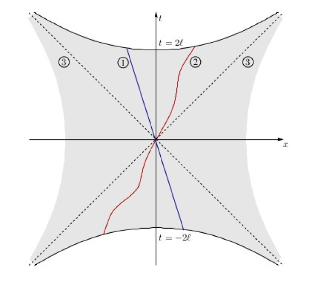
Figure 1: Projective conformal representation of de Sitter spacetime. Note that the “observer” spacetime is the interior of the Cayley-Klein absolute $t^{2}-\mathbf{x}^{2}=4\ell^{2}$.

In Figure 1 we can see that all timelike curves (2) and lightlike (1) starts in the “past horizon” and end on the “future horizon”. More details in [22].

3 Linearization of the Casimir Invariants of the spin${}_{4,1}^{e}$ Lie algebra

The classical angular momentum biform of a free particle following a “timelike” curve $\sigma$ with momentum $1$-form $\boldsymbol{p}$ in the structure $\mathbb{R}^{4,1}$ is

$$\boldsymbol{l=x}\wedge\boldsymbol{p},$$ (7)

where

$$\boldsymbol{x=X}^{A}\boldsymbol{\mathring{E}}_{A},~{}~{}~{}~{}~{}\boldsymbol{p}=P_{A}\boldsymbol{\mathring{E}}^{A}$$ (8)

are respectively the position 1-form and the momentum of the free particle. Moreover, $\{\boldsymbol{\mathring{E}}^{A}=dX^{A}\}$ is an orthonormal cobasis of $T^{\ast}\mathring{M}$ dual to the orthonormal basis $\{\boldsymbol{\mathring{e}}_{A}=\frac{\partial}{\partial X^{A}}\}$ of $T\mathring{M}$. and $\{\boldsymbol{\mathring{E}}_{A}\}$ is an orthonormal cobasis of $T^{\ast}\mathring{M},$ called the reciprocal basis of $\{\boldsymbol{\mathring{E}}^{A}\}$ and it is $\mathtt{\mathring{g}}(\boldsymbol{\mathring{E}}^{A},\boldsymbol{\mathring{E}}_{B})=\delta_{B}^{A}$ where

$$\mathtt{\mathring{g}}=\eta^{AB}\boldsymbol{\mathring{e}}_{A}\otimes\boldsymbol{\mathring{e}}_{B}$$ (9)

is the metric for $T^{\ast}\mathring{M}$. If

$$\boldsymbol{\mathring{g}}=\eta_{AB}\boldsymbol{\mathring{E}}^{A}\otimes\boldsymbol{\mathring{E}}^{B}$$ (10)

is the metric of $T\mathring{M}$, it is $\eta^{AC}\eta_{CB}=\delta_{B}^{A}$. We have

$$\boldsymbol{l}=\frac{1}{2}L_{AB}\boldsymbol{\mathring{E}}^{A}\wedge\boldsymbol{\mathring{E}}^{B}=\frac{1}{2}L_{AB}\boldsymbol{\mathring{E}}^{A}\boldsymbol{\mathring{E}}^{B}$$ (11)

with

$$L_{AB}=\eta_{AC}X^{C}P_{B}-\eta_{BC}X^{C}P_{A}$$ (12)

Remark 1

It is quite obvious that for a classical particle living in de Sitter spacetime and following a timelike worldline $\sigma$ parametrized by proper time $\tau$ if we write [15, 16]

$$\boldsymbol{x}=X^{A}(\tau)\boldsymbol{\mathring{E}}_{A}\text{,~{}~{}~{}~{}}\boldsymbol{p}=m\frac{dX^{A}(\tau)}{d\tau}\boldsymbol{\mathring{E}}_{A}$$ (13)

it is (since $\boldsymbol{x\cdot x=\mathring{g}}(\boldsymbol{x},\boldsymbol{x})=\ell^{2}$)

$$\boldsymbol{x\cdot p}=0.$$ (14)

Thus,

$$\boldsymbol{xp=x}\wedge\boldsymbol{p}$$ (15)

and as a consequence

$$\boldsymbol{l}^{2}=\boldsymbol{xpxp}=-\boldsymbol{pxxp}=-\ell^{2}\boldsymbol{p}^{2}$$ (16)

which implies that

$$\boldsymbol{l\wedge l}=0$$ (17)

and thus

$$\boldsymbol{l}^{2}=\boldsymbol{l\lrcorner l}\text{.}$$ (18)

As we re going to see the classical condition given by Eq.(17) cannot be assumed in quantum theory where the classical angular momentum is substituted by a quantum angular momentum operator.

So, to continue we define $\mathcal{\mathring{H}}$, the Hilbert space of a one quantum spin $1/2$ particle living $\mathring{M}$ as the set of all square integrable mappings

$$\phi\in\sec\mathcal{C\ell}^{0}\mathcal{(}\mathring{M},\mathtt{\mathring{g}}\mathcal{)}$$ (19)

called representatives in $\mathcal{C\ell}^{0}\mathcal{(}\mathring{M},\mathtt{\mathring{g}}\mathcal{)}$ relative to a spin coframe of (DHSF) [7].

The quantum angular momentum operator $\mathbf{L}\in\mathcal{L(\mathring{H})}$ is

$$\mathbf{L:}=\frac{1}{2}\boldsymbol{\mathring{E}}^{A}\boldsymbol{\mathring{E}}^{B}\mathbf{L}_{AB}$$ (20)

where

$$\mathbf{L}_{AB}=\eta_{AC}X^{C}\mathbf{P}_{B}-\eta_{BC}X^{C}\mathbf{P}_{A}$$ (21)

with $\mathbf{P}_{A}\in\mathcal{L(\mathring{H})}$ defined by

$$\mathbf{P}_{A}\phi:=\partial_{A}\phi\boldsymbol{\mathring{E}}^{2}\boldsymbol{\mathring{E}}^{1}$$ (22)

Now,

$$\mathbf{L}^{2}=\mathbf{L\lrcorner L+L\wedge L.}$$ (23)

$\mathbf{L\lrcorner L}$ is clearly a scalar invariant under the action of $\mathrm{Spin}_{4,1}^{e}$ group and it is:

$$\mathbf{L\lrcorner L} =\frac{1}{4}L_{AB}L^{CD}(\boldsymbol{\mathring{E}}^{A}\wedge\boldsymbol{\mathring{E}}^{B})\lrcorner(\boldsymbol{\mathring{E}}_{C}\wedge\boldsymbol{\mathring{E}}_{D})$$

$$=\frac{1}{4}L_{AB}L^{CD}\boldsymbol{\mathring{E}}^{A}\lrcorner(\boldsymbol{\mathring{E}}^{B}\lrcorner(\boldsymbol{\mathring{E}}_{C}\wedge\boldsymbol{\mathring{E}}_{D}))$$

$$=\frac{1}{4}L_{AB}L^{CD}\boldsymbol{\mathring{E}}^{A}\lrcorner(\delta_{C}^{B}\boldsymbol{\mathring{E}}_{D}-\delta_{D}^{B}\boldsymbol{\mathring{E}}_{C})$$

$$=\frac{1}{4}L_{AB}L^{CD}(\delta_{C}^{B}\delta_{D}^{A}-\delta_{D}^{B}\delta_{C}^{A})$$

$$=-\frac{1}{2}L_{AB}L^{AB}.$$ (24)

The first Casimir operator of the Lie algebra $\mathrm{spin}_{4,1}^{e}$ is defined by

$$C_{1}=\frac{1}{\ell^{2}}\mathbf{L\lrcorner L}=-\frac{1}{\ell^{2}}\mathbf{L\cdot L=}-\frac{1}{2\ell^{2}}L_{AB}L^{AB}=m^{2},$$ (25)

with $m^{2}\in\mathbb{R}$.

We have the

Proposition 2

Call

$$\mathbf{W:=}\star\frac{1}{8\ell}(\mathbf{L\wedge L})=\frac{1}{8\ell}(\mathbf{L\wedge L})\lrcorner\tau.$$ (26)

Then,

$$\mathbf{W\cdot W} =\mathbf{WW}=-\frac{1}{64\ell^{2}}(\mathbf{L\wedge L})\lrcorner(\mathbf{L\wedge L})=-\frac{1}{64\ell^{2}}(\mathbf{L\wedge L})\cdot(\mathbf{L\wedge L})$$

$$=-\frac{1}{64\ell^{2}}(\mathbf{L\wedge L})(\mathbf{L\wedge L}).$$ (27)

Proof. Recalling the identity

$$A_{l}\lrcorner\star B_{s}=B_{s}\lrcorner\star A_{l}~{}~{}\text{ if }l+s=n=\dim\mathring{M},$$

$$A_{l}\in\sec{\textstyle\bigwedge\nolimits^{l}}T^{\ast}\mathring{M}\hookrightarrow\mathcal{C\ell(}\mathring{M},\mathtt{\mathring{g}}\mathcal{)~{}~{}}\text{ }B_{s}\in\sec{\textstyle\bigwedge\nolimits^{s}}T^{\ast}\mathring{M}\hookrightarrow\mathcal{C\ell(}\mathring{M},\mathtt{\mathring{g}}\mathcal{)}$$ (28)

and taking also into account that

$$\star^{-1}A_{1}=-\star A_{1}$$ (29)

we can write

$$(\mathbf{L\wedge L})\lrcorner(\mathbf{L\wedge L}) =(\mathbf{L\wedge L})\lrcorner\star^{-1}\star(\mathbf{L\wedge L})$$

$$-(\mathbf{L\wedge L})\lrcorner\star\star(\mathbf{L\wedge L}) =-\star(\mathbf{L\wedge L})\lrcorner\star(\mathbf{L\wedge L})$$

$$=-((\mathbf{L\wedge L})\lrcorner\tau)\lrcorner((\mathbf{L\wedge L})\lrcorner\tau)$$

$$=-64\ell^{2}\mathbf{W\cdot W.}$$ (30)

On the other hand we have that

$$(\star^{-1}\mathbf{W)(\star^{-1}\mathbf{W})}=(\star\mathbf{W)(\star\mathbf{W})=W}\tau\tau\mathbf{W=-WW=-W\cdot W}$$ (31)

and since $\star^{-1}\mathbf{W=L\wedge L}$ we have from Eqs. (30) and (31) that

$$(\mathbf{L\wedge L})(\mathbf{L\wedge L})=-64\ell^{2}\mathbf{W\cdot W}=(\mathbf{L\wedge L})\lrcorner(\mathbf{L\wedge L})$$ (32)

which completes the proof.   

Remark 3

The second Casimir invariant of spin${}_{4,1}^{e}$ is defined by

$$C_{2}=\mathbf{W\cdot W}=-\frac{1}{64\ell^{2}}(\mathbf{L\wedge L})(\mathbf{L\wedge L})=-m^{2}s(s+1),$$ (33)

where $s=0,1/2,1,3/2,...$ It is thus quite obvious that contrary to the classical case the operator $\mathbf{L\wedge L}$ cannot be null for otherwise from Eq.(33) it would be necessary that $m=0$ or $s=0.$

Observe that the spin $1/2$  wave function needs to satisfy the fourth order equation

$$\left(\frac{1}{64\ell^{2}}(\mathbf{L\wedge L})(\mathbf{L\wedge L})-m^{2}s(s+1)\right)\phi=0.$$ (34)

We can factorize  the invariant $C_{2}$ as

$$\left(\frac{1}{8\ell}\mathbf{L\wedge L}+m\sqrt{s(s+1)}\right)\left(\frac{1}{8\ell}\mathbf{L\wedge L}-m\sqrt{s(s+1)}\right)=0.$$ (35)

Then, a possible second order equation that we will impose to be satisfied by $\phi$ is

$$\left(\mathbf{L\wedge L}-4\sqrt{3}m\ell\right)\phi=0.$$ (36)

To continue observe that we cannot factorize $\mathbf{L\lrcorner L}-\ell^{2}m^{2}=0$ in two first order operators. However taking into account Eq.(23) we can write

$$\frac{1}{\ell^{2}}\mathbf{L}^{2}-m^{2}-\frac{1}{\ell^{2}}\mathbf{L\wedge L}=0.$$ (37)

Thus, taking into account Eq.(36) we can write

$$\left(\frac{1}{\ell^{2}}\mathbf{L}^{2}-m^{2}\right)\phi=\frac{1}{\ell^{2}}(\mathbf{L\wedge L)}\phi=\frac{4\sqrt{3}m}{\ell}\phi,$$ (38)

or

$$\left(\frac{1}{\ell^{2}}\mathbf{L}^{2}-m^{2}-\frac{4\sqrt{3}m}{\ell}\right)\phi=0$$ (39)

and calling

$$\boldsymbol{\lambda}^{2}:=m^{2}+\frac{4\sqrt{3}m}{\ell}$$ (40)

we can now factor Eq.(39) as

$$\left(\frac{1}{\ell^{2}}\mathbf{L}^{2}-\boldsymbol{\lambda}^{2}\right)\phi=\left(\frac{1}{\ell}\mathbf{L+}\boldsymbol{\lambda}\right)\left(\frac{1}{\ell}\mathbf{L}-\boldsymbol{\lambda}\right)\phi=0.$$ (41)

3.1 The Tangency Condition and the DHESS1

Let $\{\boldsymbol{\mathring{\theta}}^{0},\boldsymbol{\mathring{\theta}}^{1},\boldsymbol{\mathring{\theta}}^{2},\boldsymbol{\mathring{\theta}}^{3},\boldsymbol{\mathring{\theta}}^{4}\}$ be an orthonormal basis for ${\textstyle\bigwedge\nolimits^{1}}T^{\ast}\mathring{M}$ such that $\{\boldsymbol{\theta}^{\mu}=\boldsymbol{\mathring{\theta}}^{\mu},~{}~{}~{}\mu=0,1,2,3\}$ is a tangent cotetrad basis for de Sitter spacetime, i.e., $\boldsymbol{\theta}^{\mu}$ $\in\sec{\textstyle\bigwedge\nolimits^{1}}T^{\ast}M\hookrightarrow\sec\mathcal{C\ell}(M,\boldsymbol{g})\subset\sec\mathcal{C\ell}(\mathring{M},\boldsymbol{\mathring{g}})$ with $\boldsymbol{\mathring{\theta}}^{4}$ orthogonal to $M$, i.e., $\boldsymbol{\mathring{\theta}}^{4}\lrcorner\tau_{\boldsymbol{g}}=0$.

We now propose taking into account Eq.(41) that the electron wave function in de Sitter spacetime must satisfy the linear equation

$$\left(\frac{1}{\ell}\mathbf{L}-\boldsymbol{\lambda}\right)\phi=0,$$ (42)

with the constrain that $\phi$ is tangent to $M$, i.e., it does not contain in its expansion terms containing $\boldsymbol{\mathring{\theta}}^{A}\boldsymbol{\mathring{\theta}}^{4}$.

Eq.(42) will be called the Dirac-Hestenes equation in de Sitter spacetime (DHESS1).

Remark 4

Take notice that in our formalism $\boldsymbol{\lambda}^{2}$ must be necessarily be a real number. Thus, if we had choose as wave equation from the factorization of Eq.(34) the equation

$$\left(\mathbf{L\wedge L}+4\sqrt{3}m\ell\right)\phi=0.$$ (43)

we would get $\boldsymbol{\lambda}^{2}=m(m-\frac{4\sqrt{3}}{\ell})\geq 0$ and would arrive at the conclusion that the theory implies that all particles living in de Sitter manifold would have masses satisfying $m\geq\frac{4\sqrt{3}}{l}$!. This will be investigate in another publication.

Remark 5

We make the important observation that if we did not use Eq.(36), a constraint coming for the factorization of the second Casimir invariant $C_{2}$, then factorization of Eq.(37) leads (taking into account that $\star^{-1}\mathbf{W=L\wedge L}$) to the integro-differential equation

$$\left(\frac{1}{\ell}\mathbf{L}-\sqrt{m^{2}+\star^{-1}\frac{1}{\ell^{2}}\mathbf{W}}\right)\phi=0.$$ (44)

Remark 6

Note that the matrix representation of Eq.(41) in terms of the representatives $\Phi\in\sec\mathbf{P}_{\mathrm{Spin}_{4,1}^{e}}(\mathring{M},\mathtt{\mathring{g})}\times\mathbb{C}^{4}$ of $\phi$ is

$$\left(\frac{1}{\ell}\underline{L}-\boldsymbol{\lambda}\right)\Phi=0,~{}~{}~{}~{}\underline{L}:=\underline{\gamma}^{A}\underline{\gamma}^{B}\mathbf{L}_{AB}$$ (45)

In Eq.(45) $\underline{\gamma}^{A}$ is a matrix representation of $\theta^{A}$, $A=1,2,3,4,0$. Note that since the operator $\underline{L}$ is not Hermitian in [6] the author left open the possibility that $\boldsymbol{\lambda}$ is a complex number. This is not the case in our formalism, as we already observed in Remark 4.

4 An Heuristic Derivation of the DHESS2

We start recalling that a classical free particle in de Sitter manifold structure $(M,\boldsymbol{g})$ certainly follows a timelike worldline $\sigma:\mathbb{R}\supset I\rightarrow M$. To unveil the nature of that motion we suppose the existence of a 2-form field $\boldsymbol{L}\in\sec{\textstyle\bigwedge\nolimits^{2}}T^{\ast}\mathring{M}\hookrightarrow\sec\mathcal{C\ell}((\mathring{M},\boldsymbol{\mathring{g}})$ such that its restriction over $\sigma$ is $\boldsymbol{l}$ i.e., $\boldsymbol{L}_{\mid\sigma}=\boldsymbol{l}$. given by Eq.(11).

It is a very reasonable hypothesis that the classical motion of a free particle in de Sitter manifold structure $(M,\boldsymbol{g})$ will happen only under the condition that $\boldsymbol{L}\in\sec{\textstyle\bigwedge\nolimits^{2}}T^{\ast}\mathring{M}\hookrightarrow\sec\mathcal{C\ell}((\mathring{M},\boldsymbol{\mathring{g}})$ is a constant $2$-form $\boldsymbol{B}$ as registered by an hypothetical “observer” living in the bulk spacetime structure $\mathbb{R}^{4,1}$. This is an obvious generalization of the fact that the free motion of a classical particle in the Minkowski spacetime structure (see Appendix D) happens with constant momentum. Let $\{\boldsymbol{\mathring{\theta}}^{A},~{}A=0,1,2,3,4\}$ be an orthonormal basis for ${\textstyle\bigwedge\nolimits^{1}}T^{\ast}\mathring{M}$ such that $\{\boldsymbol{\theta}^{\mu}=\boldsymbol{\mathring{\theta}}^{\mu},~{}\mu=0,1,2,3\}$ is a cotetrad basis for ${\textstyle\bigwedge\nolimits^{1}}T^{\ast}M\hookrightarrow\mathcal{C\ell}(M,\mathtt{g})\subset\mathcal{C\ell}(\mathring{M},\mathtt{\mathring{g}})$ with $\boldsymbol{\mathring{\theta}}^{4}$ orthogonal to $M$, i.e., $\boldsymbol{\mathring{\theta}}^{4}\lrcorner\tau_{\boldsymbol{g}}=0$. Then, the condition that $\boldsymbol{L}$ is a constant $2$-form may be written

$$\frac{1}{\ell}\boldsymbol{L}=-\kappa\boldsymbol{B}.$$ (46)

Now, let $\phi^{\prime}$ be an invertible DHSF living in $(\mathring{M},\boldsymbol{\mathring{g})}$ such that

$$\boldsymbol{B}=\phi^{\prime-1}\boldsymbol{\mathring{\theta}}^{1}\boldsymbol{\mathring{\theta}}^{2}\phi^{\prime}=\boldsymbol{\mathring{E}}^{1}\boldsymbol{\mathring{E}}^{2}.$$ (47)

Before continuing we also suppose that

$$\phi^{\prime-1}\boldsymbol{\mathring{\theta}}^{A}\boldsymbol{\mathring{\theta}}^{B}\phi^{\prime}=\boldsymbol{\mathring{E}}^{A}\boldsymbol{\mathring{E}}^{B},~{}~{}~{}A,B=0,1,2,3,4.$$ (48)

Using Eq.(47) in Eq.(46) we can write a purely classic DHESS equation, namely,

$$\frac{1}{\ell}\boldsymbol{L}\phi^{\prime-1}\boldsymbol{\mathring{\theta}}^{2}\boldsymbol{\mathring{\theta}}^{1}=-\kappa\phi^{\prime-1}.$$ (49)

This is compatible with a quantum DHESS1, i.e.,

$$\frac{1}{\ell}\mathbf{L}\phi^{\prime-1}+\kappa\phi^{\prime-1}=0$$ (50)

with the postulate that when we restrict our considerations to DHSFs living in the de Sitter structure $(M,\boldsymbol{g})$ it is:

$$\frac{1}{\ell}\boldsymbol{L}\phi^{\prime-1}\boldsymbol{\mathring{\theta}}^{2}\boldsymbol{\mathring{\theta}}^{1}\mapsto\frac{1}{\ell}\mathbf{L}\phi^{\prime-1}:=\boldsymbol{\mathring{\theta}}^{A}\boldsymbol{\mathring{\theta}}^{B}\left(X_{A}\mathbf{P}_{B}-X_{B}\mathbf{P}_{A}\right)\phi^{\prime-1}$$ (51)

with

$$\boldsymbol{P}_{A}\phi^{\prime-1}\mapsto\mathbf{P}_{A}\phi^{\prime-1}:=\frac{\partial}{\partial X^{A}}\phi^{\prime-1}\boldsymbol{\mathring{\theta}}^{2}\boldsymbol{\mathring{\theta}}^{1}.$$ (52)

Note that under the above conditions the DHESS1 equation (Eq.(42)) will be identical to the DHESS2 (Eq.(50)) if

$$\lambda\mapsto\kappa,~{}~{}~{}~{}\phi^{\prime-1}\mapsto\phi.$$ (53)

Indeed, recall that a generalization of a DHSF (see Eq.(104) in Appendix B ) for the $(\mathring{M}\simeq\mathbb{R}^{5},\boldsymbol{\mathring{g}})$ structure (see page 106 of[7]) can be written as

$$\phi^{\prime}=\rho^{1/2}U,~{}~{}~{}\phi^{\prime}=\rho^{-1/2}U^{-1}$$ (54)

where $\rho$ is a scalar function $U\in\sec\mathcal{C\ell}^{0}\mathcal{(}\mathring{M},\boldsymbol{\mathring{g})}$ and for any $x\in\mathring{M}$, $U(x)\tilde{U}(x)=1$. Note that $U$ can be written as

$$U(x)=e^{z(x)F(x)}=(\cosh z(x)+F(x)\sinh z(x))$$ (55)

with the $2$-form $F$ satisfying $F^{2}=1$. Under these conditions a standard calculation shows that

$$\frac{\partial\phi^{\prime^{-1}}}{\partial X^{M}}\phi^{\prime}=-\phi^{\prime^{-1}}\frac{\partial\phi^{\prime}}{\partial X^{M}}=\phi^{\prime}\frac{\partial\phi^{\prime-1}}{\partial X^{M}},~{}~{}M=0,1,2,3,4.$$ (56)

Thus, starting with Eq.(42) and writing $\boldsymbol{\mathring{\theta}}^{A}\boldsymbol{\mathring{\theta}}^{B}=\phi^{\prime}\boldsymbol{\mathring{E}}^{A}\boldsymbol{\mathring{E}}^{B}\phi^{\prime-1}$we get

$$0 =\boldsymbol{\mathring{\theta}}^{A}\boldsymbol{\mathring{\theta}}^{B}\left(X_{A}\boldsymbol{P}_{B}-X_{B}\boldsymbol{P}_{A}\right)\phi^{\prime-1}+\kappa\phi^{\prime-1}$$

$$=-\phi^{\prime}\boldsymbol{\mathring{E}}^{A}\boldsymbol{\mathring{E}}^{B}\phi^{\prime-1}\left[\left(X_{A}\frac{\partial}{\partial X^{B}}-X_{B}\frac{\partial}{\partial X^{A}}\right)\phi^{\prime-1}\right]\phi^{\prime}\boldsymbol{\mathring{E}}^{2}\boldsymbol{\mathring{E}}^{1}\phi^{\prime-1}+\kappa\phi^{\prime-1}$$

$$=-\phi^{\prime}\boldsymbol{\mathring{E}}^{A}\boldsymbol{\mathring{E}}^{B}\phi^{\prime-1}\left[\phi^{\prime}\left(X_{A}\frac{\partial}{\partial X^{B}}-X_{B}\frac{\partial}{\partial X^{A}}\right)\phi^{\prime-1}\right]\boldsymbol{\mathring{E}}^{2}\boldsymbol{\mathring{E}}^{1}\phi^{\prime-1}+\kappa\phi^{\prime-1}$$

$$=-\phi^{\prime}\boldsymbol{\mathring{E}}^{A}\boldsymbol{\mathring{E}}^{B}\left[\left(X_{A}\frac{\partial}{\partial X^{B}}-X_{B}\frac{\partial}{\partial X^{A}}\right)\phi^{\prime-1}\right]\boldsymbol{\mathring{E}}^{2}\boldsymbol{\mathring{E}}^{1}\phi^{\prime^{-1}}+\kappa\phi^{\prime-1}$$ (57)

and multiplying Eq.(57) on the left by $\phi^{\prime-1}$ and on the right by $\phi$ we get

$$0=\boldsymbol{\mathring{E}}^{A}\boldsymbol{\mathring{E}}^{B}\left[\left(X_{A}\frac{\partial}{\partial X^{B}}-X_{B}\frac{\partial}{\partial X^{A}}\right)\phi^{\prime-1}\right]\boldsymbol{\mathring{E}}^{2}\boldsymbol{\mathring{E}}^{1}-\kappa\phi^{\prime-1}.$$ (58)

which taking into account Eq.(53) is identical to Eq.(42).

5 The limit $\ell\rightarrow\infty$ of Eq.(50)

Expressing $\mathbf{L}_{AB}$ in terms of the projective coordinates we get

$$\mathbf{L}_{\alpha 4}\phi=l\partial_{\alpha}\phi\boldsymbol{\mathring{\theta}}^{2}\boldsymbol{\mathring{\theta}}^{1}-\frac{1}{4l}(2\eta_{\alpha\lambda}x^{\lambda}x^{\nu}-\sigma^{2}\delta_{\alpha}^{\nu})\partial_{\nu}\phi\boldsymbol{\mathring{\theta}}^{2}\boldsymbol{\mathring{\theta}}^{1}.$$ (59)

Also,

$$\mathbf{L}_{\mu\nu}\phi=-\eta_{\mu\lambda}x^{\lambda}\partial_{\nu}\phi\boldsymbol{\mathring{\theta}}^{2}\boldsymbol{\mathring{\theta}}^{1}+\eta_{\nu\lambda}x^{\lambda}\partial_{\mu}\phi\boldsymbol{\mathring{\theta}}^{2}\boldsymbol{\mathring{\theta}}^{1}$$ (60)

Taking into account the results of Appendix B (Eq.(125) and Remark 21 ) we know that $\phi$ must be of the form

$$\phi=\left(\varphi+\boldsymbol{\mathring{\theta}}_{4}\boldsymbol{\mathring{\theta}}_{\alpha}\xi^{\alpha}\right)\in\sec\mathcal{C\ell}^{0}\mathcal{(}\mathring{M},\boldsymbol{\mathring{g}}\mathcal{)}$$ (61)

with $\varphi$ living in a particular ideal of $\mathcal{C\ell}^{0}\mathcal{(}\mathring{M},\boldsymbol{\mathring{g}}\mathcal{)}$. Moreover, taking into account that in Eq.(125) the $\mathbf{\xi}^{\alpha}$, $\alpha=0,1,2,3$ must be linked in order to define only three degrees of freedom we take $\eta_{\alpha\beta}\xi^{\alpha}\tilde{\xi}^{\beta}=1$. Recalling that $\eta_{\alpha\beta}X^{\alpha}X^{\beta}=\ell^{2}(1-(X^{4})^{2}/\ell^{2})$ we have $\eta_{\alpha\beta}x^{\alpha}x^{\beta}=-\frac{\ell^{2}}{\Omega^{2}}(1-\frac{(X^{4})^{2}}{\ell^{2}})$ and a possible solution for our constraint is

$$\xi^{\alpha}=\frac{1}{\ell}\Omega^{2}x^{\alpha}\lambda$$ (62)

where $\lambda$ $\in\mathcal{C\ell}^{0}\mathcal{(}\mathring{M},\boldsymbol{\mathring{g}}\mathcal{)}$ is such that $\lambda\tilde{\lambda}=-1/(1-(X^{4})^{2}/\ell^{2})$. Thus $\phi$ can be written as

$$\phi=\varphi+\frac{1}{\ell}\Omega^{2}\boldsymbol{\mathring{\theta}}_{4}\boldsymbol{\mathring{\theta}}_{\alpha}x^{\alpha}\lambda$$ (63)

and Eq.(51) can be written (in the limit $\ell\rightarrow\infty$) as

$$\boldsymbol{\mathring{\theta}}^{\alpha}\boldsymbol{\mathring{\theta}}^{4}\frac{\partial}{\partial x^{\alpha}}\varphi\boldsymbol{\mathring{\theta}}^{2}\boldsymbol{\mathring{\theta}}^{1}-\boldsymbol{\lambda}\varphi=0.$$ (64)

Now, calling $\boldsymbol{\mathring{\theta}}^{\alpha}\boldsymbol{\mathring{\theta}}^{4}=\Gamma^{\alpha}$, $\alpha=0,1,2,3$ we know (see AppendixD) that

$$\Gamma^{\alpha}\Gamma^{\beta}+\Gamma^{\beta}\Gamma^{\alpha}=2\eta^{\alpha\beta}.$$ (65)

Finally, recalling Eq.(63) we can write Eq.(64) in the limit $\ell\rightarrow\infty$ as

$$\Gamma^{\alpha}\frac{\partial}{\partial x^{\alpha}}\varphi\Gamma^{2}\Gamma^{1}-m\varphi=0.$$ (66)

which is clearly a representative of the DHE in Minkowski spacetime in the $\mathcal{C\ell(}M\simeq\mathbb{R}^{4},\boldsymbol{\eta}\mathcal{)}$ bundle which reads

$$\gamma^{\alpha}\frac{\partial}{\partial x^{\alpha}}\psi\gamma^{2}\gamma^{1}-m\psi\gamma^{0}=0.$$ (67)

Indeed, multiplying Eq.(67) on the right by the idempotent $\frac{1}{2}(1+\gamma^{0})$ it reads (calling $\zeta=\psi\frac{1}{2}(1+\gamma^{0})$)

$$\gamma^{\alpha}\frac{\partial}{\partial x^{\alpha}}\zeta\gamma^{2}\gamma^{1}-m\zeta=0.$$ (68)

So, Eqs. (66) and (67) can be identified with the identifications

$$\Gamma^{\alpha}\leftrightarrow\gamma^{\alpha},~{}~{}~{}~{}~{}\varphi\leftrightarrow\zeta$$ (69)

Remark 7

It is well known that when $\ell\rightarrow\infty$ the $\mathbf{DHESS1}$ (Eq.(42))  which is a Clifford bundle representation of the Dirac equation (written with the standard matrix formalism) is also equivalent to the $\mathbf{DHE}$ in Minkowski spacetime [6].

6 Conclusions

We gave a Clifford bundle motivated approach to the wave equation of a free spin $1/2$ fermion in the de Sitter manifold, a brane with topology $M=\mathrm{S0}(4,1)/\mathrm{S0}(3,1)$ living in the bulk spacetime $\mathbb{R}^{4,1}=(\mathring{M}=\mathbb{R}^{5},\boldsymbol{\mathring{g}})$ and equipped with a metric field $\boldsymbol{g:}=-i^{\ast}\mathring{g}$ with $\boldsymbol{i}:M\rightarrow\mathring{M}$ being the inclusion map. To obtain the analog of Dirac equation in Minkowski spacetime we appropriately factorize the two Casimir invariants $C_{1}$ and $C_{2}$ of the Lie algebra of the de Sitter group using the constraint given in the linearization of $C_{2}$ as input to linearize $C_{1}$. In this way we obtain an equation that we called DHESS1 (which is simply postulated in previous studies ([4, 6]). Next we derive a wave equation (called DHESS2) for a free spin $1/2$ fermion in the de Sitter manifold using an heuristic argument which is an obvious generalization of an heuristic argument (described in detail in one of the appendices) permitting a derivation of the Dirac equation in Minkowski spacetime which shows that such famous equation express nothing more that the momentum of a free particle is a constant vector field over timelike  integral curves of a given velocity field.  It is a nice fact that DHESS1 and DHESS2 coincide. We emphasize moreover that our approach leaves clear the nature and meaning of the Casimir invariants [2] and thus of the object $\boldsymbol{\lambda}$ (Eq.(40)), something that is not clear in other papers on the subject such as, e.g., [4, 6, 12, 14] which use the standard covariant Dirac spinor fields.

As a last comment here we recall that if the de Sitter manifold is supposed to be a spacetime, i.e., a structure[19] $(M,\boldsymbol{g}$,$\tau_{\boldsymbol{g}},\nabla,\uparrow)$ where $\nabla$ is an arbitrary connection compatible with $\boldsymbol{g}$ then the writing of Dirac equation in such a structure is supposed to  be given by very different arguments from the ones used in this paper. A comparison of the two approaches will be presented elsewhere.

Acknowledgement 8

M. Rivera-Tapia and E. A. Notte-Cuello were supported by the Direccion de Investigación de la Universidad de La Serena DIULS. The work of I. Kondrashuk was supported by Fondecyt (Chile) Grants Nos. 1040368, 1050512, and 1121030, and by DIUBB (Chile) Grants Nos. 102609 and 121909 GI/C-UBB. S. A. Wainer is grateful to CAPES for a Ph.D. fellowship.

Appendix A SO${}^{e}(4,1)$ and Spin${}_{4,1}^{e}$ and their Lie Algebras

The group O$(4,1)$ may be defined as the group of (invertible) $5\times 5$ real matrices $\mathbf{\Lambda}$ such that if $\mathbf{X}^{t}=(X^{1},X^{2},X^{3},X^{4},X^{0})$ denotes a $1\times 5$ real matrix and if

$$\boldsymbol{\mathring{G}=}\left(\begin{array}[c]{ccccc}1&0&0&0&0\\ 0&1&0&0&0\\ 0&0&1&0&0\\ 0&0&0&1&0\\ 0&0&0&0&-1\end{array}\right)$$ (70)

then

$$\mathbf{\Lambda}^{t}\boldsymbol{\mathring{G}}\mathbf{\Lambda}=\boldsymbol{\mathring{G}.}$$ (71)

Of, course, $\det\mathbf{\Lambda}^{2}=1$. Let O${}^{\uparrow}(4,1)$ be the subgroup of O$(4,1)$ such that if $\mathbf{X}^{t}=(X^{1},X^{2},X^{3},X^{4},X^{0})$ and $X^{0}>0$ then $(\mathbf{\Lambda X)}^{t}=(X^{\prime 1},X^{\prime 2},X^{\prime 3},X^{{}^{\prime}4},X^{\prime 0})$ has $X^{\prime 0}>0.$

The matrices with $\det\Lambda=1$ closes the subgroup SO${}_{+}(4,1)$ of O$(4,1)$. The elements of SO${}_{+}(4,1)$ are clearly connected to the identity element of O$(4,1)$. We shall denoted by SO${}^{e}(4,1)=$ O${}^{\uparrow}(4,1)\cap$SO${}_{+}(4,1)$. We denote by Spin${}_{4,1}^{e}$the simple connected group that is the double cover of SO${}^{e}(4,1)$. It is a well known result [13] that the elements of Spin${}_{4,1}^{e}$ are the invertible elements of $u\in\mathbb{R}_{4,1}^{0}$ such that $u\tilde{u}=1$.

Now, it is a well known result that the elements of SO${}^{e}(4,1)$ can be written as an exponential of a sum of antisymmetric matrices $\mathbf{M}_{AB}$, i.e.,

$$\mathbf{\Lambda=}\exp\left(\frac{1}{2}\chi^{AB}\mathbf{M}_{AB}\right),~{}~{}~{}~{}~{}\chi^{AB}=-\chi^{BA},~{}~{}~{}~{}\chi^{AB}\in\mathbb{R}\text{.}$$ (72)

The matrices $\mathbf{M}_{AB}$ closes the Lie algebra so${}^{e}(4,1)$ of SO${}_{+}(4,1)$ and satisfy the commutation relations

$$[\mathbf{M}_{AB},\mathbf{M}_{CD}]=\eta_{AC}\mathbf{M}_{BD}+\eta_{BD}\mathbf{M}_{AC}-\eta_{BC}\mathbf{M}_{AD}-\eta_{AD}\mathbf{M}_{BC}.$$ (73)

When SO${}_{+}(4,1)$ acts as a transformation group in the manifold $\mathring{M}$ the generators $\mathbf{M}_{AB}$ of the Lie algebra so${}^{e}(4,1)$ are represented by the vector fields

$$\mathbf{\xi}_{AB}=\eta_{AC}X^{C}\frac{\partial}{\partial X^{B}}-\eta_{BC}X^{C}\frac{\partial}{\partial X^{A}}$$ (74)

which are Killing vector fields of $\boldsymbol{\mathring{g}}$, i.e., $\pounds_{\mathcal{\xi}_{AB}}\boldsymbol{\mathring{g}}=0$, with $\pounds$ denoting the Lie derivative. Of course, if $f:\mathring{M}\rightarrow\mathbb{R}$ we immediately verify that

$$[\mathbf{\xi}_{AB},\mathbf{\xi}_{CD}]f=(\eta_{AC}\mathbf{\xi}_{BD}+\eta_{BD}\mathbf{\xi}_{AC}-\eta_{BC}\mathbf{\xi}_{AD}-\eta_{AD}\mathbf{\xi}_{BC})f.$$ (75)

On the other hand the elements of Spin${}_{4,1}^{e}$ are of the form $\pm\exp\mathbf{B}$ where $\mathbf{B}$ is a biform. We write $u\in$Spin${}_{4,1}^{e}$ as

$$u=\exp\left(\frac{1}{4}\chi_{AB}\boldsymbol{\mathring{E}}^{AB}\right)=\exp\left(\frac{1}{4}\chi_{AB}\boldsymbol{\mathring{E}}^{A}\boldsymbol{\mathring{E}}^{B}\right)$$ (76)

and we may immediately verify that the biforms $\mathbf{S}^{AB}=\frac{1}{2}\boldsymbol{\mathring{E}}^{AB}$ satisfy the Lie algebra spin${}_{4,1}^{e}$which is isomorphic to the Lie algebra so${}^{e}(4,1)$, i.e.

$$[\mathbf{S}_{AB},\mathbf{S}_{CD}]=\eta_{AC}\mathbf{S}_{BD}+\eta_{BD}\mathbf{S}_{AC}-\eta_{BC}\mathbf{S}_{AD}-\eta_{AD}\mathbf{S}_{BC}.$$ (77)

Appendix B DHSF

In this Appendix for convenience for the reader we recall the definition of the concept of DHSF for a generic $4$-dimensional spin manifold $M$ equipped with a metric $\boldsymbol{g}$. The presentation improves a lit bit the theory as developed originally in [18, 11, 9].

In what follows $\mathbf{P}_{\mathrm{SO}_{1,3}^{e}}(M,\boldsymbol{g})$ ($P_{\mathrm{SO}_{1,3}^{e}}(M,\mathtt{g})$) denotes the principal bundle of oriented Lorentz tetrads (cotetrads).

Definition 9

A spin structure for a general $m$-dimensional manifold $M$ consists of a principal fiber bundle $\pi_{s}:P_{\mathrm{Spin}_{p,q}^{e}}(M,\mathtt{g})\rightarrow M$, (called the Spin Frame Bundle) with group $\mathrm{Spin}_{p,q}^{e}$ and a map

$$\Lambda:P_{\mathrm{Spin}_{p,q}^{e}}(M,\mathtt{g})\rightarrow P_{\mathrm{SO}_{p,q}^{e}}(M,\mathtt{g}),$$ (78)

satisfying the following conditions:

(i)

$\pi(\Lambda(p))=\pi_{s}(p),\forall p\in P_{\mathrm{Spin}_{p,q}^{e}}(M,\mathtt{g})$, where $\pi$ is the projection map of the bundle $\pi:P_{\mathrm{SO}_{p,q}^{e}}(M,\mathtt{g})\rightarrow M$.

(ii)

$\Lambda(pu)=\Lambda(p)\mathrm{Ad}_{u},\forall p\in P_{\mathrm{Spin}_{p,q}^{e}}(M,\mathtt{g})$ and $\mathrm{Ad}:\mathrm{Spin}_{p,q}^{e}\rightarrow\mathrm{SO}_{p,q}^{e},\break\mathrm{Ad}_{u}(a)=uau^{-1}.$

Definition 10

Any section of $P_{\mathrm{Spin}_{p,q}^{e}}(M,\mathtt{g})$ is called a spin frame field (or simply a spin frame). We shall use the symbol $\Xi\in\sec P_{\mathrm{Spin}_{p,q}^{e}}(M,\mathtt{g})$ to denoted a spin frame.

We know that [19]:

$$\mathcal{C}\ell(M,\mathtt{g})=P_{\mathrm{SO}_{1,3}^{e}}(M,\mathtt{g})\times_{\rho}\mathbb{R}_{1,3}=P_{\mathrm{Spin}_{1,3}^{e}}(M,\mathtt{g})\times_{Ad}\mathbb{R}_{1,3},$$ (79)

and since $\bigwedge TM\hookrightarrow\mathcal{C}\ell(M,\mathtt{g})$, sections of $\mathcal{C}\ell(M,\mathtt{g})$ (the Clifford fields) can be represented as a sum of non homogeneous differential forms.

Next, using that $M\simeq S^{3}\times\mathbb{R\subset}\mathring{M}$ is parallelizable, we introduce the global tetrad basis $\boldsymbol{e}_{\alpha},\alpha=0,1,2,3$ on $TM$ and in $T^{\ast}M$ the cotetrad basis on $\{\boldsymbol{\gamma}^{\alpha}\}$, which are dual basis. We introduce the reciprocal basis $\{\boldsymbol{e}^{\alpha}\}$ and $\{\boldsymbol{\gamma}_{\alpha}\}$ of $\{\boldsymbol{e}_{\alpha}\}$ and $\{\boldsymbol{\gamma}^{\alpha}\}$ satisfying

$$\boldsymbol{g}(\boldsymbol{e}_{\alpha},\boldsymbol{e}^{\beta})=\delta_{\alpha}^{\beta},~{}~{}~{}\mathtt{g}(\boldsymbol{\gamma}^{\beta},\boldsymbol{\gamma}_{\alpha})=\delta_{\alpha}^{\beta}.$$ (80)

Moreover, recall that

$$\boldsymbol{g}=\eta_{\alpha\beta}\boldsymbol{\gamma}^{\alpha}\otimes\boldsymbol{\gamma}^{\beta}=\eta^{\alpha\beta}\boldsymbol{\gamma}_{\alpha}\otimes\boldsymbol{\gamma}_{\beta},~{}~{}~{}\mathtt{g}=\eta^{\alpha\beta}\boldsymbol{e}_{\alpha}\otimes\boldsymbol{e}_{\beta}=\eta_{\alpha\beta}\boldsymbol{e}^{\alpha}\otimes\boldsymbol{e}^{\beta}.$$ (81)

In this work we have that exists a spin structure on the 4-dimensional Lorentzian manifold $(M,\boldsymbol{g})$, since $M$ is parallelizable, i.e., $P_{\mathrm{SO}_{1,3}^{e}}(M,\mathtt{g})$ is trivial, because of the following result due to Geroch [5]:

Theorem 11

For a $4-$dimensional Lorentzian manifold$\ (M,\boldsymbol{g})$, a spin structure exists if and only if $P_{\mathrm{SO}_{1,3}^{e}}(M,\mathtt{g})$ is a trivial bundle.

The basis $\left.\boldsymbol{\gamma}^{\alpha}\right|_{p}$ of $T_{p}M\simeq\mathbb{R}^{1,3},p\in M$, generates the algebra $\mathcal{C}\ell(T_{p}M,\mathtt{g})\simeq\mathbb{R}_{1,3}$. We have that [19]

$$\mathrm{e}=\frac{1}{2}(1+\boldsymbol{\gamma}^{0})\in\mathbb{R}_{1,3}$$

is a primitive idempotent of $\mathbb{R}_{1,3}$ and

$$\mathrm{f}=\frac{1}{2}(1+\boldsymbol{\gamma}^{0})\frac{1}{2}(1+i\boldsymbol{\gamma}^{2}\boldsymbol{\gamma}^{1})\in\mathbb{C\otimes R}_{1,3}$$

is a primitive idempotent of $\mathbb{C\otimes R}_{1,3}$. Now, let $I=\mathbb{R}_{1,3}\mathrm{e}$ and $I_{\mathbb{C}}=\mathbb{C\otimes R}_{1,3}\mathrm{f}$ be respectively the minimal left ideals of $\mathbb{R}_{1,3}$ and $\mathbb{C\otimes R}_{1,3}$ generated by $\mathrm{e}$ and $\mathrm{f}$. Any $\phi\in I$ can be written as

$$\phi=\psi\mathrm{e}$$

with $\psi\in\mathbb{R}_{1,3}^{0}$. Analogously, any $\mathbf{\phi}\in I_{\mathbb{C}}$ can be written as

$$\psi\mathrm{e}\frac{1}{2}(1+i\boldsymbol{\gamma}^{2}\boldsymbol{\gamma}^{1})$$

with $\psi\in\mathbb{R}_{1,3}^{0}.$ Recall moreover that $\mathbb{C\otimes R}_{1,3}\simeq\mathbb{R}_{4,1}\simeq\mathbb{C}(4)$. We can verify that

$$\left(\begin{array}[c]{cccc}1&0&0&0\\ 0&0&0&0\\ 0&0&0&0\\ 0&0&0&0\end{array}\right)$$

is a primitive idempotent of $\mathbb{C}(4)$ which is a matrix representation of $\mathrm{f}$. In that way, there is a bijection between column spinors, i.e., elements of $\mathbb{C}^{4}$ and the elements of $I_{\mathbb{C}}$.

Recalling that $\mathrm{Spin}_{1,3}^{e}\hookrightarrow\mathbb{R}_{1,3}^{0}$, we give:

Definition 12

The left (respectively right) real spin-Clifford bundle of the spin manifold $M$ is the vector bundle $\mathcal{C}\ell_{\mathrm{Spin}}^{l}(M,\mathtt{g})=P_{\mathrm{Spin}_{1,3}^{e}}(M,\mathtt{g})\times_{l}\mathbb{R}_{1,3}$ (respectively $\mathcal{C}\ell_{\mathrm{Spin}}^{r}(M,\mathtt{g})=P_{\mathrm{Spin}_{1,3}^{e}}(M,\mathtt{g})\times_{r}\mathbb{R}_{1,3}$) where $l$ is the representation of $\mathrm{Spin}_{1,3}^{e}$ on $\mathbb{R}_{1,3}$ given by $l(a)x=ax$ (respectively, where $r$ is the representation of $\mathrm{Spin}_{1,3}^{e}$ on $\mathbb{R}_{1,3}$ given by $r(a)x=xa^{-1}$). Sections of $\mathcal{C}\ell_{\mathrm{Spin}}^{l}(M,\mathtt{g})$ are called left spin-Clifford fields (respectively right spin-Clifford fields).

Definition 13

Let $\mathbf{e,f}\in\mathcal{C}\ell_{\mathrm{Spin}_{1,3}^{e}}^{l}(M,\mathtt{g})$ be a primitive global idempotents , respectively $\mathbf{e^{r}}\in\mathcal{C}\ell_{\mathrm{Spin}_{1,3}^{e}}^{r}(M,\mathtt{g})$, and let $I(M,\mathtt{g})$ be the subbundle of $\mathcal{C}\ell_{\mathrm{Spin}_{1,3}^{e}}^{l}(M,\mathtt{g})$ generated by the idempotent, that is, if $\mathbf{\Psi}$ is a section of $I(M,\mathtt{g})\subset\mathcal{C}\ell_{\mathrm{Spin}_{1,3}^{e}}^{l}(M,\mathtt{g})$, we have

$$\mathbf{\Psi e}=\mathbf{\Psi},$$ (82)

A section $\mathbf{\Psi}$ of $I(M,\mathtt{g})$ is called a left ideal algebraic spinor field.

Definition 14

A Dirac-Hestenes spinor field (DHSF) associated with $\mathbf{\Psi}$ is a section $\varPsi$ of $\mathcal{C}\ell_{\mathrm{Spin}_{1,3}^{e}}^{0l}(M,\mathtt{g})\subset\mathcal{C}\ell_{\mathrm{Spin}_{1,3}^{e}}^{l}(M,\mathtt{g})$ such that

$$\mathbf{\Psi}=\varPsi\mathbf{e}.$$ (83)

Definition 15

We denote the complexified left spin-Clifford bundle by

$$\mathbb{C}\ell_{\mathrm{Spin}_{1,3}^{e}}^{l}(M,\mathtt{g})=P_{\mathrm{Spin}_{1,3}^{e}}(M,\mathtt{g})\times_{l}\mathbb{C}\otimes\mathbb{R}_{1,3}\equiv P_{\mathrm{Spin}_{1,3}^{e}}(M,\mathtt{g})\times_{l}\mathbb{R}_{1,4}.$$

Definition 16

An equivalent definition of a DHSF is the following. Let $\mathbf{\Psi}\in\sec\mathbb{C}\ell_{\mathrm{Spin}_{1,3}^{e}}^{l}(M,\mathtt{g})$ such that

$$\mathbf{\Psi f=\Psi.}$$

Then a DHSF associated with $\mathbf{\Psi}$ is an even section $\varPsi$ of $\mathcal{C}\ell_{\mathrm{Spin}_{1,3}^{e}}^{0l}(M,\mathtt{g})\subset\mathcal{C}\ell_{\mathrm{Spin}_{1,3}^{e}}^{l}(M,\mathtt{g})$ such that

$$\mathbf{\Psi}=\varPsi\mathbf{f}.$$ (84)

Definition 17

There are natural pairings:

$$\sec\mathcal{C}\ell_{\mathrm{Spin}_{1,3}^{e}}^{l}(M,\mathtt{g})\times\sec\mathcal{C}\ell_{\mathrm{Spin}_{1,3}^{e}}^{r}(M,\mathtt{g}) \rightarrow\sec\mathcal{C}\ell(M,\mathtt{g}),$$ (85)

$$\sec\mathcal{C}\ell_{\mathrm{Spin}_{1,3}^{e}}^{r}(M,\mathtt{g})\times\sec\mathcal{C}\ell_{\mathrm{Spin}_{1,3}^{e}}^{l}(M,\mathtt{g}) \rightarrow\mathcal{F(}M,\mathbb{R}_{1,3}),$$ (86)

such that given a section $\alpha$ of $\mathcal{C}\ell_{\mathrm{Spin}_{1,3}^{e}}^{l}(M,\mathtt{g})$ and a section $\beta$ of $\mathcal{C}\ell_{\mathrm{Spin}_{1,3}^{e}}^{r}(M,\mathtt{g})$ and selecting representatives $(p,a)$ for $\alpha(x)$ and $(p,b)$ for $\beta(x)$ ($p\in\pi^{-1}\left(x\right)$) it is

$$(\alpha\beta) :=[(p;ab)]\in\mathcal{C}\ell(M,\mathtt{g}),$$ (87)

$$(\beta\alpha)(x) :=ba\in\mathbb{R}_{1,3}.$$ (88)

If alternative representatives $(pu^{-1},ua)$ and $(pu^{-1},bu^{-1})$ are chosen for $\alpha(x)$ and $\beta(x)$ we have $[(pu^{-1};uabu^{-1})]$, that, by Eq.(79) represents the same element on $\mathcal{C}\ell(M,\mathtt{g})$, and $(bu^{-1}ua)=ba$; thus $(\alpha\beta)(x)$ and $(\beta\alpha)(x)$ are a well defined. Following the same procedure we can define the actions:

$$\sec\mathcal{C}\ell(M,\mathtt{g})\times\sec\mathcal{C}\ell_{\mathrm{Spin}_{1,3}^{e}}^{l}(M,\mathtt{g}) \rightarrow\sec\mathcal{C}\ell_{\mathrm{Spin}_{1,3}^{e}}^{l}(M,\mathtt{g}),$$ (89)

$$\sec\mathcal{C}\ell_{\mathrm{Spin}_{1,3}^{e}}^{r}(M,\mathtt{g})\times\sec\mathcal{C}\ell(M,\mathtt{g}) \rightarrow\sec\mathcal{C}\ell_{\mathrm{Spin}_{1,3}^{e}}^{r}(M,\mathtt{g}),$$ (90)

$$\sec\mathcal{C}\ell_{\mathrm{Spin}_{1,3}^{e}}^{l}(M,\mathtt{g})\times\mathbb{R}_{1,3} \rightarrow\sec\mathcal{C}\ell_{\mathrm{Spin}_{1,3}^{e}}^{l}(M,\mathtt{g}),$$ (91)

$$\mathbb{R}_{1,3}\times\sec\mathcal{C}\ell_{\mathrm{Spin}_{1,3}^{e}}^{r}(M,\mathtt{g}) \rightarrow\sec\mathcal{C}\ell_{\mathrm{Spin}_{1,3}^{e}}^{r}(M,\mathtt{g}).$$ (92)

Given a local trivialization of $\mathcal{C}\ell(M,\mathtt{g})$ (or $\mathcal{C}\ell_{\mathrm{Spin}_{1,3}^{e}}^{l}(M,\mathtt{g})$, $\mathcal{C}\ell_{\mathrm{Spin}_{1,3}^{e}}^{r}(M,\mathtt{g}),$ $\mathbb{C}\ell_{\mathrm{Spin}_{p,q}^{e}}^{l}(M,\mathtt{g})$) ($\mathcal{U}\subset M$)

$$\phi_{U}:\pi^{-1}(\mathcal{U})\rightarrow\mathcal{U}\times\mathbb{R}_{1,3},$$ (93)

we can define a local unit section by $\mathbf{1}_{U}(x)=\phi_{U}^{-1}(x,1)$. For $\mathcal{C}\ell(M,\mathtt{g})$, it is easy to show that a global unit section always exist, independently of the fact that $M$  is parallelizable or not. For the bundles $\mathcal{C}\ell_{\mathrm{Spin}_{p,q}^{e}}^{l}(M,\mathtt{g})$, $\mathcal{C}\ell_{\mathrm{Spin}_{p,q}^{e}}^{r}(M,\mathtt{g})$, $\mathbb{C}\ell_{\mathrm{Spin}_{p,q}^{e}}^{l}(M,\mathtt{g})$ ($\dim$ $M=p+q$) there exist a global unit sections if, and only if, $P_{\mathrm{Spin}_{p,q}^{e}}(M,\mathtt{g})$ is trivial [18, 11, 19]. In our case we know, that $M$ is parallelizable and we can define global unit sections on $\mathcal{C}\ell_{\mathrm{Spin}_{1,3}^{e}}^{l}(M,\mathtt{g})$, $\mathcal{C}\ell_{\mathrm{Spin}_{1,3}^{e}}^{r}(M,\mathtt{g})$ and $\mathbb{C}\ell_{\mathrm{Spin}_{1,3}^{e}}^{r}(M,\mathtt{g})$.

Let $\boldsymbol{\mathbf{\Xi}}$_u be a section of $P_{\mathrm{Spin}_{1,3}^{e}}(M,\mathtt{g})$, i.e., a spin frame. We recall, in order to fix notations, that sections of $\mathcal{C}\ell(M,\mathtt{g})$ $I^{l}(M,\mathtt{g})$, $\mathcal{C}\ell_{\mathrm{Spin}_{1,3}^{e}}^{l}(M,\mathtt{g})$, are, respectively, the equivalence classes

$$\boldsymbol{C}=[(\boldsymbol{\mathbf{\Xi}}_{u},\mathcal{C}_{\boldsymbol{\mathbf{\Xi}}_{u}})],$$

$$\mathbf{\Psi}=[(\boldsymbol{\mathbf{\Xi}}_{u},\boldsymbol{\Psi}_{\boldsymbol{\mathbf{\Xi}}_{u}})],~{}~{}~{}\varPsi=[(\boldsymbol{\mathbf{\Xi}}_{u},\varPsi_{\boldsymbol{\mathbf{\Xi}}_{u}})].$$ (94)

Remark 18

When convenient, we will write $\mathcal{C}_{\Xi_{u}}\in\sec\mathcal{C}\ell(M,\mathtt{g})$ to mean that there exists a section $\boldsymbol{C}$ of the Clifford bundle $\mathcal{C}\ell(M,\mathtt{g})$ defined by $[(\boldsymbol{\mathbf{\Xi}}_{u},\mathcal{C}_{\boldsymbol{\mathbf{\Xi}}_{u}})]$. Analogous notations will be used for sections of the other bundles introduced above. Also, when there is no chance of confusion on the chosen spinor frame, we will write $\mathcal{C}_{\boldsymbol{\mathbf{\Xi}}_{u}}$ simply as $\mathcal{C}$.

For each spin frame, say $\boldsymbol{\mathbf{\Xi}}$₀, let $\mathbf{1}_{\boldsymbol{\mathbf{\Xi}}_{0}}^{l}$ and $\mathbf{1}_{\boldsymbol{\mathbf{\Xi}}_{0}}^{r}$ be the global unit sections of $\mathcal{C\ell}_{\mathrm{Spin}_{1,3}^{e}}^{l}(M,\mathtt{g})$ and $\mathcal{C\ell}_{\mathrm{Spin}_{1,3}^{e}}^{r}(M,\mathtt{g})$, given by

$$\mathbf{1}_{\boldsymbol{\mathbf{\Xi}}_{0}}^{r}:=[(\Xi_{0},1)],~{}~{}~{}~{}~{}\mathbf{1}_{\boldsymbol{\mathbf{\Xi}}_{0}}^{l}:=[(\Xi_{0},1)].$$ (95)

Remark 19

Before proceeding note that given another spin frame $\Xi_{u}=\Xi_{0}u$, where $u:M\rightarrow\mathrm{Spin}_{1,3}^{e}\subset\mathbb{R}_{1,3}^{0}\subset\mathbb{R}_{1,3}$ we define the sections $\mathbf{1}_{\boldsymbol{\mathbf{\Xi}}_{u}}^{r}$ of $\mathcal{C\ell}_{\mathrm{Spin}_{1,3}^{e}}^{r}(M,\mathtt{g})$ and $\mathbf{1}_{\boldsymbol{\mathbf{\Xi}}_{0}}^{l}$ of $\mathcal{C\ell}_{\mathrm{Spin}_{1,3}^{e}}^{l}(M,\mathtt{g})$ by

$$\mathbf{1}_{\boldsymbol{\mathbf{\Xi}}_{u}}^{r}:=[(\Xi_{u},1)],~{}~{}~{}~{}~{}\mathbf{1}_{\boldsymbol{\mathbf{\Xi}}_{u}}^{l}:=[(\Xi_{u},1)].$$ (96)

It has been proved in [18, 19] that the relation between $\mathbf{1}_{\boldsymbol{\mathbf{\Xi}}}^{r}$ and $\mathbf{1}_{\boldsymbol{\mathbf{\Xi}}_{0}}^{r}$ and between $\mathbf{1}_{\boldsymbol{\mathbf{\Xi}}}^{l}$ and $\mathbf{1}_{\boldsymbol{\mathbf{\Xi}}_{0}}^{l}$ are given by

$$\mathbf{1}_{\boldsymbol{\mathbf{\Xi}}_{u}}^{r}=u^{-1}\mathbf{1}_{\boldsymbol{\mathbf{\Xi}}_{0}}^{r}=\mathbf{1}_{\boldsymbol{\mathbf{\Xi}}_{0}}^{r}U^{-1},~{}~{}~{}~{}~{}\mathbf{1}_{\boldsymbol{\mathbf{\Xi}}_{u}}^{l}=U\mathbf{1}_{\boldsymbol{\mathbf{\Xi}}_{0}}^{l}=\mathbf{1}_{\boldsymbol{\mathbf{\Xi}}_{0}}^{l}u$$ (97)

where $U$ is the section of $\mathcal{C}\ell(M,\mathtt{g})$ defined by the equivalence class

$$U=[(\Xi_{0},u)].$$ (98)

The unity sections $\mathbf{1}_{\boldsymbol{\mathbf{\Xi}}_{u}}^{l}$ and $\mathbf{1}_{\boldsymbol{\mathbf{\Xi}}_{u}}^{r}$satisfies the important relations

$$\mathbf{1}_{\boldsymbol{\mathbf{\Xi}}_{u}}^{l}\mathbf{1}_{\boldsymbol{\mathbf{\Xi}}_{u}}^{r}=1\in\sec\mathcal{C}\ell(M,\mathtt{g}),~{}\mathbf{1}_{\boldsymbol{\mathbf{\Xi}}_{u}}^{r}\mathbf{1}_{\boldsymbol{\mathbf{\Xi}}_{u}}^{l}=1\in\mathcal{F(}M,\mathbb{R}_{1,3}),$$ (99)

Definition 20

A representative of a DHSF $\varPsi$ in the Clifford bundle $\mathcal{C}\ell(M,\mathtt{g})$ relative to a spin frame $\mathbf{\Xi}_{u}$ is a section $\boldsymbol{\psi}_{\mathbf{\Xi}_{u}}=[(\mathbf{\Xi}_{u},\psi_{\mathbf{\Xi}_{u}})]$ of $\mathcal{C}\ell^{0}(M,\mathtt{g})$ given by [18, 11, 19]

$$\boldsymbol{\psi}_{\mathbf{\Xi}_{u}}=\Psi\mathbf{1}_{\mathbf{\Xi}_{u}}^{r},.$$ (100)

Representatives in the Clifford bundle of $\varPsi$ relative to spin frames, say $\mathbf{\Xi}_{u^{\prime}}$ and $\mathbf{\Xi}_{u}$, are related by

$$\boldsymbol{\psi}_{\mathbf{\Xi}_{u^{\prime}}}U^{\prime-1}=\boldsymbol{\psi}_{\mathbf{\Xi}_{u}}U^{-1}.$$ (101)

In the main text we use the symbol $\phi$ as a short for the representative of a DHSF in the spinor basis defined by the fiducial frame $\Xi_{0}$.

DHSFs unveil the hidden geometrical meaning of spinors (and spinor fields). Indeed, consider $v\in\mathbb{R}^{1,3}\hookrightarrow\mathbb{R}_{1,3}$ be, initially, a timelike covector such that $v^{2}=1.$ The linear mapping, belonging to $\mathrm{SO}_{1,3}^{e}$

$$v\mapsto RvR^{-1}=Rv\tilde{R}=w,~{}R\in\mathrm{Spin}_{1,3}^{e},$$ (102)

define a new covector $w$ such that $w^{2}=1.$ We can therefore fix a covector $v$ and obtain all other unit timelike covectors by applying this mapping. This same procedure can be generalized to obtain any type of timelike covector starting from a fixed unit covector $v$. We define the linear mapping

$$v\mapsto\psi v\tilde{\psi}=z$$ (103)

to obtain $z^{2}=\rho^{2}>0$. Since $z$ can be written as $z=\rho Rv\tilde{R}$, we need

$$\psi v\tilde{\psi}=\rho Rv\tilde{R}.$$ (104)

If we write  $\psi=\rho^{\frac{1}{2}}MR$ we need that $Mv\tilde{M}=v$ and the most general solution is $M=e^{\frac{\tau_{\boldsymbol{g}}\beta}{2}}$, where $\tau_{\boldsymbol{g}}=\gamma^{0}\gamma^{1}\gamma^{2}\gamma^{3}\in{\textstyle\bigwedge\nolimits^{4}}\mathbb{R}^{1,3}\hookrightarrow\mathbb{R}_{1,3}$ and $\beta\in\mathbb{R}$ is called the Takabayasi angle [19, 23]. Then follows that $\psi$ is of the form

$$\psi=\rho^{\frac{1}{2}}e^{\frac{\tau_{\boldsymbol{g}}\beta}{2}}R.$$ (105)

Now, Eq.(105) shows that $\psi\in\mathbb{R}_{1,3}^{0}\simeq\mathbb{R}_{3,0}$. Moreover, we have that $\psi\tilde{\psi}\neq 0$ since

$$\psi\tilde{\psi}=\rho e^{\tau_{\boldsymbol{g}}\beta}=(\rho\cos\beta)+\tau_{\boldsymbol{g}}(\rho\sin\beta).$$ (106)

A representative of a DHSF $\varPsi$ in the Clifford bundle $\mathcal{C}\ell(M,\mathtt{g})$ relative to a spin frame $\mathbf{\Xi}_{u}$ is a section $\boldsymbol{\psi}_{\mathbf{\Xi}_{u}}=[(\mathbf{\Xi}_{u},\psi_{\mathbf{\Xi}_{u}})]$ of $\mathcal{C}\ell^{0}(M,\mathtt{g})$ where $\psi_{\mathbf{\Xi}_{u}}\in\mathbb{R}_{1,3}^{0}\simeq\mathbb{R}_{3,0}$. So a DHSF such $\boldsymbol{\psi}_{\mathbf{\Xi}_{u}}\boldsymbol{\tilde{\psi}}_{\mathbf{\Xi}_{u}}\neq 0$ induces a linear mapping induced by Eq.(103), which rotates a covector field and dilate it.

Appendix C Description of the Dirac Equation in the Clifford Bundle

To fix the notation let $(M\simeq\mathbb{R}^{4},\boldsymbol{\eta},D,\tau_{\mathbf{\eta}})$ be the Minkowski spacetime structure where $\boldsymbol{\eta}\in\sec T_{0}^{2}M$ is Minkowski metric and $D$ is the Levi-Civita connection of $\boldsymbol{\eta}$. Also, $\tau_{\mathbf{\eta}}\in\sec{\textstyle\bigwedge\nolimits^{4}}T^{\ast}M$ defines an orientation. We denote by $\mathtt{\eta}\in\sec T_{2}^{0}M$ the metric of the cotangent bundle. It is defined as follows. Let $\{x^{\mu}\}$ be coordinates for $M$ in the Einstein-Lorentz-Poincaré gauge [19]. Let $\{\boldsymbol{e}_{\mu}=\partial/\partial x^{\mu}\}$ a basis for $TM$ and $\{\gamma^{\mu}=dx^{\mu}\}$ the corresponding dual basis for $T^{\ast}M$, i.e., $\gamma^{\mu}(\boldsymbol{e}_{\alpha})=\delta_{\alpha}^{\mu}$. Then, if $\boldsymbol{\eta}=\eta_{\mu\nu}\gamma^{\mu}\otimes\gamma^{\nu}$ then $\mathtt{\eta}=\eta^{\mu\nu}\boldsymbol{e}_{\mu}\otimes\boldsymbol{e}_{\nu}$, where the matrix with entries $\eta_{\mu\nu}$ and the one with entries $\eta^{\mu\nu}$ are the equal to the diagonal matrix $\mathrm{diag}(1,-1,-1,-1)$. If $a,b\in\sec{\textstyle\bigwedge\nolimits^{1}}T^{\ast}M$ we write $a\cdot b=\mathtt{\eta}(a,b)$. We also denote by $\langle\gamma_{\mu}\rangle$ the reciprocal basis of $\{\gamma^{\mu}=dx^{\mu}\}$, which satisfies $\gamma^{\mu}\cdot\gamma_{\nu}=\delta_{\nu}^{\mu}$.

We denote the Clifford bundle of differential forms in Minkowski spacetime by $\mathcal{C\ell}(M,\eta)$ and use notations and conventions in what follows as in [19] and recall the fundamental relation

$$\gamma^{\mu}\gamma^{\nu}+\gamma^{\nu}\gamma^{\mu}=2\eta^{\mu\nu}.$$ (107)

If $\{\boldsymbol{\gamma}^{\mu},~{}$ $\mu=0,1,2,3\}$ are the Dirac gamma matrices in the standard representation and $\{\gamma_{\mu},~{}\mu=0,1,2,3\}$ are as introduced above, we define

$$\sigma_{k} :=\gamma_{k}\gamma_{0}\in\sec{\textstyle\bigwedge\nolimits^{2}}T^{\ast}M\hookrightarrow\sec\mathcal{C\ell}^{0}(M,\eta)\text{, }k=1,2,3,$$ (108)

$$\mathbf{i} =\gamma_{5}:=\gamma_{0}\gamma_{1}\gamma_{2}\gamma_{3}\in\sec{\textstyle\bigwedge\nolimits^{4}}T^{\ast}M\hookrightarrow\sec\mathcal{C\ell}(M,\eta),$$ (109)

$$\boldsymbol{\gamma}_{5} :=\boldsymbol{\gamma}_{0}\boldsymbol{\gamma}_{1}\boldsymbol{\gamma}_{2}\boldsymbol{\gamma}_{3}\in\mathbb{C(}4\mathbb{)}$$ (110)

Noting that $M$ is parallelizable, in a given global spin frame a covariant spinor field can be taken as a mapping $\boldsymbol{\psi}:M\rightarrow\mathbb{C}^{4}$  In standard representation of the gamma matrices where ($i=\sqrt{-1}$, $\boldsymbol{\phi},\boldsymbol{\varsigma}:M\rightarrow\mathbb{C}^{2}$) to $\boldsymbol{\psi}$ given by

$$\boldsymbol{\psi}=\left(\begin{array}[c]{c}\boldsymbol{\phi}\\ \boldsymbol{\varsigma}\end{array}\right)=\left(\begin{array}[c]{c}\left(\begin{array}[c]{c}m^{0}+im^{3}\\ -m^{2}+im^{1}\end{array}\right)\\ \left(\begin{array}[c]{c}n^{0}+in^{3}\\ -n^{2}+in^{1}\end{array}\right)\end{array}\right),$$ (111)

there corresponds the DHSF $\psi\in\sec\mathcal{C\ell}^{0}(M,\eta)$ given by

$$\psi=\phi+\varsigma\sigma_{3}=(m^{0}+m^{k}\mathbf{i}\sigma_{k})+(n^{0}+n^{k}\mathbf{i}\sigma_{k})\sigma_{3}.$$ (112)

We then have the useful formulas in Eq.(113) below that one can use to immediately translate results of the standard matrix formalism in the language of the Clifford bundle formalism and vice-versa

$$\boldsymbol{\gamma}_{\mu}\boldsymbol{\psi} \leftrightarrow\gamma_{\mu}\psi\gamma_{0},$$

$$i\boldsymbol{\psi} \leftrightarrow\psi\gamma_{21}=\psi\mathbf{i}\sigma_{3},$$

$$i\boldsymbol{\gamma}_{5}\boldsymbol{\psi} \leftrightarrow\psi\sigma_{3}=\psi\gamma_{3}\gamma_{0},$$

$$\boldsymbol{\bar{\psi}} =\boldsymbol{\psi}^{\dagger}\boldsymbol{\gamma}^{0}\leftrightarrow\tilde{\psi},$$

$$\boldsymbol{\psi}^{\dagger} \leftrightarrow\gamma_{0}\tilde{\psi}\gamma_{0},$$

$$\boldsymbol{\psi}^{\ast} \leftrightarrow-\gamma_{2}\psi\gamma_{2}.$$ (113)

Using the above dictionary the standard Dirac equation for a Dirac spinor field $\boldsymbol{\psi}:M\rightarrow\mathbb{C}^{4}$

$$i\boldsymbol{\gamma}^{\mu}\partial_{\mu}\boldsymbol{\psi}-m\boldsymbol{\psi}=0$$ (114)

translates immediately in the so-called Dirac-Hestenes equation, i.e.,

$$\boldsymbol{\partial}\psi\gamma_{21}-m\psi\gamma_{0}=0.$$ (115)

Appendix D Generalized Dirac-Hestenes Spinors for $\mathbb{R}_{4,1}$

Let $\{\boldsymbol{E}^{A}\}$, $a=1,2,3,4,0$ be an orthonormal basis for $\mathbb{R}_{4,1}$. We have

$$\boldsymbol{E}^{A}\boldsymbol{E}^{B}+\boldsymbol{E}^{B}\boldsymbol{E}^{A}=2\eta^{AB}$$ (116)

where the matrix with entries $\eta^{AB}$ is the diagonal matrix diag$(1,1,1,1,-1).$Define $\mathfrak{i:=}\boldsymbol{E}^{0}\boldsymbol{E}^{1}\boldsymbol{E}^{2}\boldsymbol{E}^{3}\boldsymbol{E}^{4}$ and $\Gamma^{\mu}=\boldsymbol{E}^{\mu}\boldsymbol{E}^{4}$. Then,

$$\Gamma^{\mu}\Gamma^{\nu}+\Gamma^{\nu}\Gamma^{\mu}=2\eta^{\mu\nu}$$ (117)

where the matrix with entries $\eta^{\mu\nu}$ is the diagonal matrix diag$(1,-1,-1,-1)$. Recalling that $\mathbb{R}_{4,1}\simeq\mathbb{C\otimes R}_{1,3}\simeq\mathbb{C\otimes R}_{3,1}$ and that

$$f=\frac{1}{2}(1+\Gamma^{0})\frac{1}{2}(1+\mathfrak{i}\Gamma^{2}\Gamma^{1})$$ (118)

is a primitive idempotent of $\mathbb{R}_{4,1}$ and $I=\mathbb{R}_{4,1}f$ is a minimum ideal of $\mathbb{R}_{4,1}$ such that $\dim_{\mathbb{R}}I=8$. Let $\Psi\in\mathbb{R}_{4,1}f$ and $Z\in\mathbb{R}_{4,1}^{0}\frac{1}{2}(1+\Gamma^{0})$. Since $\mathbb{R}_{4,1}^{0}\simeq\mathbb{R}_{1,3}$ we recognize $Z$ as isomorphic to some covariant Dirac spinor. We can easily find the following relation between $\Psi$ and $Z$

$$\Psi=Z\frac{1}{2}(1+\mathfrak{i}\Gamma^{2}\Gamma^{1}).$$ (119)

Moreover, decomposing $Z$ into even and odd parts relative to the $\mathbb{Z}_{2}$-gradation of $\mathbb{R}_{4,1}^{0}\simeq\mathbb{R}_{1,3}$, $Z=Z^{0}+Z^{1}$ we find that $Z^{1}=Z^{0}\Gamma^{0}$, which clearly shows that all information in $Z$ is contained in $Z^{0}$. Then, we have

$$\Psi=Z^{0}(1+\Gamma^{0})\frac{1}{2}(1+\mathfrak{i}\Gamma^{2}\Gamma^{1})$$ (120)

Now, taking into account the well known result that

$$\mathbb{R}_{4,1}^{0}\frac{1}{2}(1+\Gamma^{0})=\mathbb{R}_{4,1}^{00}\frac{1}{2}(1+\Gamma^{0})$$ (121)

where $\mathbb{R}_{4,1}^{00}\simeq\mathbb{R}_{1,3}^{0}$ is the even subalgebra of $\mathbb{R}_{4,1}^{0}\simeq\mathbb{R}_{1,3}$ we see that $Z\in\mathbb{R}_{4,1}^{0}\frac{1}{2}(1+\Gamma^{0})$ can be written as

$$Z=\psi\frac{1}{2}(1+\Gamma^{0}),~{}~{}~{}~{}$$ (122)

with $\psi\in\mathbb{R}_{4,1}^{00}\simeq\mathbb{R}_{1,3}^{0}$ a representative of a Dirac-Hestenes spinor. Thus, putting $Z^{0}=\psi/2$ we end with the notable expression

$$\Psi=\psi\frac{1}{2}(1+\Gamma^{0})\frac{1}{2}(1+\mathfrak{i}\Gamma^{2}\Gamma^{1}).$$ (123)

Next note that Hestenes (see page 106 of [7]) defines a spinor for $\mathbb{R}_{4,1}$the object

$$\boldsymbol{\Phi}=\zeta^{1/2}\mathbf{V},$$ (124)

where $\zeta$ is a scalar and $\mathbf{V}\in\mathbb{R}_{4,1}^{0}$ and $\mathbf{V\tilde{V}}=1$ such that for any $\mathbf{x}\in\mathbb{R}_{4,1}$, $\Upsilon\mathbf{x}\Upsilon\in\mathbb{R}_{4,1}$. To relate $\Upsilon$ with $\psi$ we write

$$\boldsymbol{\Phi=}\psi\frac{1}{2}(1+\Gamma^{0})+\mathbf{\xi}^{\alpha}\Gamma_{0}\Gamma_{\alpha}\in\mathbb{R}_{4,1}^{0}.$$ (125)

Remark 21

Take notice that the $\mathbf{\xi}^{\alpha}$ are four scalars which must satisfy some link in order to define the additional $3$ degrees of freedom of $\boldsymbol{\Phi}$ and $\psi\in\mathbb{R}_{4,1}^{00}\simeq\mathbb{R}_{1,3}^{0}$ such that $\psi\tilde{\psi}\neq 0$ is written as

$$\psi=\mathbf{S\ +}\frac{1}{2}\mathbf{B}_{\mu\nu}\Gamma^{\mu}\Gamma^{\nu}+\mathbf{P}\Gamma^{0}\Gamma^{1}\Gamma^{2}\Gamma^{3}=\mathbf{\rho}^{1/2}e^{-\frac{\beta\Gamma^{0}\Gamma^{1}\Gamma^{2}\Gamma^{3}}{2}}\mathbf{U}$$ (126)

with $\mathbf{U\in}\mathbb{R}_{1,3}^{0}$ such that $\mathbf{U\tilde{U}=1}$. Moreover, since $\boldsymbol{\Phi\tilde{\Phi}}=\zeta$ we need the additional link

$$\left[\psi\frac{1}{2}(1+\Gamma^{0})+\mathbf{\xi}^{\alpha}\Gamma_{0}\Gamma_{\alpha}\right]\left[\frac{1}{2}\tilde{\psi}(1-\Gamma^{0})-\mathbf{\xi}^{\alpha}\Gamma_{0}\Gamma_{\alpha}\right]=\zeta.$$ (127)

Appendix E Heuristic Derivation of the DHE in Minkowski Spacetime

We start recalling that a classical spin $1/2$ free particle is supposed to have its story described by a geodesic timelike worldline $\sigma:\mathbb{R}\supset I\rightarrow M(\approx\mathbb{R}^{4})$ in the Minkowski spacetime structure Let $\sigma_{\ast}$ be the velocity of the particle and let $\boldsymbol{v}=\boldsymbol{\eta}(\sigma_{\ast},)$ be the physically equivalent 1-form. We that $\boldsymbol{v}\in\sec T_{\sigma}^{\ast}M\hookrightarrow\sec\mathcal{C}{\ell}(M,\mathtt{\eta})$. Its classical momentum $1$-form is

$$\boldsymbol{p}=m\boldsymbol{v.}$$ (128)

To continue, we suppose the existence of a 1-form field $V\in\sec\bigwedge^{1}T^{\ast}M\hookrightarrow\sec\mathcal{C}{\ell}(M,\mathtt{g})$ such that its restriction over $\sigma$ is $\boldsymbol{v}$, i.e., $V_{\mid\sigma}=\boldsymbol{v}$. Also we impose that $V^{2}=1$. We introduce also the $\boldsymbol{P}$ vector field such that $\left.\boldsymbol{P}\right|_{\sigma}=\boldsymbol{p}$ and consider the equation

$$\boldsymbol{P}=m\boldsymbol{V}$$ (129)

As in the previous appendix, let $\psi\in\sec\mathcal{C}{\ell}^{0}(M,\mathtt{g})$, be the representative (in the spin coframe $\Xi$) of a particular invertible Dirac-Hestenes spinor field such that

$$\psi\tilde{\psi}\neq 0$$ (130)

and since $\psi=\rho^{\frac{1}{2}}e^{\frac{\beta}{2}\gamma^{5}}R$ we have

$$\psi\gamma^{0}\tilde{\psi}=\rho e^{\beta\gamma^{5}}R\gamma^{0}\tilde{R}.$$ (131)

which necessarily implies that if we want $\ V=\psi\gamma^{0}\tilde{\psi}$ we need

$$e^{\beta\gamma^{5}}=\pm 1,$$ (132)

i.e., $\beta=0$ or $\beta=\pi$. In what follows we take $\beta=0$. Thus Eq.(129) becomes

$$\boldsymbol{P}=m\psi\gamma^{0}\tilde{\psi}$$ (133)

and thus

$$\boldsymbol{P}\psi=m\psi\gamma^{0}$$ (134)

Eq.(134) is a purely classical equation which is simply another way of writing Eq.(129). To get a quantum mechanics  wave equation we must now change $\boldsymbol{P}$ into $\mathbf{P}$, the quantum mechanics momentum operator. From the previous appendix we know that

$$\mathbf{P}\psi=\boldsymbol{\partial}\psi\gamma^{2}\gamma^{1}=\gamma^{\mu}\partial_{\mu}\psi\gamma^{2}\gamma^{1}.$$ (135)

Substituting this result in Eq.(134) we get (compare with Eq.(23) of [17])

$$\boldsymbol{\partial}\psi\gamma^{2}\gamma^{1}-m\psi\gamma^{0}=0.$$ (136)

which is the DHE, which, as well known, is completely equivalent to the standard Dirac equation formulated in terms of covariant Dirac spinor fields.

References

• [1] Arcidiacono, G. , Relativitá e Cosmologia, vol. II (iv edizione), Libreira Eredi Virgilio Vechi, Roma, 1987.
• [2] Cotăescu, I. I.,  The Physical Meaning of the de Sitter Invariants, Gen  Rel. Grav. 43, 1639-1656 (2011). [arXiv:1006.1472v6 [gr-qc] ]
• [3] Crummeyrole, A., Orthogonal and Symplectic Clifford Algebras, Kluwer Acad. Publ.., Dordrecht, 1.990.
• [4] Dirac, P. A. M., The Electron Wave Equation in De-Sitter Space, Ann. Math. 36, 657-669 (1935).
• [5] Geroch, R., Spinor Structure of Space-Times in General Relativity I, J. Math. Phys. 9, 1739-1744 (1968).
• [6] Gürsey, F., Introduction to Group Theory, in DeWiit, C. and DeWiit, B. (eds.), Relativity, Groups and Topology, pp 91-161, Gordon and Breach, New York, 1964.
• [7] Hestenes D., and Sobczyk, G., Clifford Algebras to Geometrical Calculus, D. Reidel Publ. Co., Dordrecht, 1984.
• [8] Lawson, H. B. Jr. and Michelson, M-L., Spin Geometry, Princeton University Press, Princeton, 1989.
• [9] Leão, R. F. , Rodrigues, W. A. Jr. and Wainer, S. A., Concept of Lie Derivative of Spinor Fields. A Geometric Motived Approach, Adv. Applied Clifford Algebras (online first), DOI 10.1007/600006-015-0560-y [arXiv:1411.7845 [math-ph] ]
• [10] Lounesto P., Clifford Algebras and Spinors, Cambridge Univ. Press, Cambridge, 1997.
• [11] Mosna, R. A. and Rodrigues, W. A. Jr., The Bundles of Algebraic and Dirac-Hestenes Spinors and Spinor Fields,.J. Math. Phys. 45, 2908-2994 (2004). [ arXiv:math-ph/0212033 ].
• [12] Notte-Cuello, E. A. and Capelas de Oliveira, E., Klein-Gordon and Dirac Equations in de Sitter Space Time, Int. J. Theor. Phys. 38, 585-598(1999).
• [13] Porteous, I., Topological Geometry, second edition, Cambridge Univ. Press, Cambridge, 1981.
• [14] Riordan, F., Solutions of the Dirac Equation in Finite de Sitter Space 9Representations of $SO_{4,1}$), N. Cimento B 20, 309-325 (1974).
• [15] Rocha, R., Rodrigues, W. A. Jr., Diffeomorphism Invariance and Local Lorentz Invariance, Adv. Appl. Clifford Algebras. 18, 945-961 (2008).
• [16] Rocha, R., Rodrigues, W. A. Jr., Hidden Consequence of Active Local Lorentz Invariance, Int. J. Geom Meth.Mod. Phys. 2, 305-357 (2005).
• [17] Rocha, R., Rodrigues, W. A. Jr., The Dirac-Hestenes Equation for Spherical Symmetric Potentials in the Spherical and Cartesian Gauges, International Journal of Modern Physics A 21 4071-4082 (2006) .
• [18] Rodrigues, W. A. Jr., Algebraic and Dirac-Hestenes Spinors and Spinor Fields, J. Math. Phys. 45 , 2908-2994 (2004) [ arXiv:math-ph/0212030].
• [19] Rodrigues, W. A. Jr. and Capelas de Oliveira, E., The Many Faces of Maxwell, Dirac and Einstein Equation,. A Clifford Bundle Approach, Lecture Notes in Physics 722, Springer, Heidelberg, 2007. A preliminary enlarged second edition may be found at http://www.ime.unicamp.br/~walrod/svmde04092013.pdf
• [20] Rodrigues, W. A. Jr., Vaz Jr., J. and Pavsic, M., The Clifford Bundle and the Dynamics of the Superparticle, Banach Center Publications. Polish Acad. Sci. 37, 295-314 (1996).
• [21] Rodrigues, W A. Jr., and Wainer, S. A., A Clifford Bundle Approach to the Differential Geometry of Branes, Adv. Applied Clifford Algebras 24, 617-847 (2014). [arXiv:1309.4007]
• [22] Rodrigues, W A. Jr., and Wainer, S. A., Notes on Conservation Laws, Equations of Motion of Matter and Particle Fields in Lorentzian and Teleparallel de Sitter Spacetime Structures. [arXiv:1505.02935 [math-ph] ]
• [23] Vaz Jr., J., Space-Time Algebra, Dirac-Hestenes Spinors and the Theory of the Electron, Ph.D. Thesis UNICAMP (1993).