CRAB NEBULA: FIVE-YEAR OBSERVATION WITH ARGO-YBJ

Abstract

The ARGO-YBJ air shower detector monitored the Crab Nebula gamma ray emission from 2007 November to 2013 February. The integrated signal, consisting of $\sim$3.3 $\times$ 10⁵ events, reached the statistical significance of 21.1 standard deviations. The obtained energy spectrum in the energy range 0.3-20 TeV can be described by a power law function dN/dE = I₀ (E / 2 TeV)^-α, with a flux normalization I₀ = (5.2 $\pm$ 0.2) $\times$ 10^-12 photons cm^-2 s^-1 TeV^-1 and $\alpha$ = 2.63 $\pm$ 0.05, corresponding to an integrated flux above 1 TeV of 1.97 $\times$ 10^-11 photons cm^-2 s^-1. The systematic error is estimated to be less that 30$\%$ for the flux normalization and 0.06 for the spectral index. Assuming a power law spectrum with an exponential cutoff dN/dE = I₀ (E / 2 TeV)^-α $\exp$ (-E / E_cut), the lower limit of the cutoff energy E_cut is 12 TeV, at 90$\%$ confidence level. Our extended dataset allows the study of the TeV emission over long timescales. Over five years, the light curve of the Crab Nebula in 200-day bins is compatible with a steady emission with a probability of 7.3 $\times$ 10^-2. A correlated analysis with Fermi-LAT data over $\sim$4.5 years using the light curves of the two experiments gives a Pearson correlation coefficient $r$ = 0.56 $\pm$ 0.22. Concerning flux variations on timescales of days, a “blind” search for flares with a duration of 1-15 days gives no excess with a significance higher than four standard deviations. The average rate measured by ARGO-YBJ during the three most powerful flares detected by Fermi-LAT is 205 $\pm$ 91 photons day^-1, consistent with the average value of 137 $\pm$ 10 day^-1.

1. Introduction

The Crab Nebula is the remnant of a supernova exploded in 1054 A.D. at a distance of $\sim$2 kpc. It contains a 33 ms pulsar that powers a wind of relativistic particles. The interactions of these particles with the remnant gas, photons and magnetic field produce a non-thermal radiation extending from radio waves to TeV gamma rays (Bühler & Blanford,, 2014, and references therein). Most of the emission is generally attributed to synchrotron radiation of relativistic electrons and positrons. The spectral energy distribution (SED) peaks between optical and X-ray frequencies. A second component arises above $\sim$400 MeV, interpreted as Inverse Compton (IC) of the same electrons scattering off synchrotron photons and CMB photons.

The Crab Nebula is one of the most luminous sources of very high energy (VHE) gamma rays in the sky, and the first source to be detected at TeV energies (Weekes et al.,, 1989). Thanks to its high flux and apparent stability it is considered a reference source in gamma ray astronomy. Detected by many experiments, both Cherenkov telescopes (Aharonian et al.,, 2004, 2006; Albert et al.,, 2008) and air shower arrays (Amenomori et al.,, 2009; Abdo et al.,, 2012), the Crab Nebula was often used to check the detector performance, including sensitivity, pointing accuracy and angular resolution.

In 2010 September the AGILE satellite unexpectedly detected a strong flare from the direction of the Crab Nebula at energies above 100 MeV. It lasted two days, with a maximum flux three times higher than the average value (Tavani et al.,, 2011), later confirmed by Fermi (Abdo et al.,, 2011). From then on, Fermi and AGILE reported some more flares, characterized by a rapid increase and decay of the flux, typically lasting a few days. The most impressive occurred in 2011 April, when the observed flux was $\sim$10 times higher than usual (Buehler et al.,, 2012). The measured SED shows a new spectral component emerging during flares, peaking at high energies (up to hundreds MeVs in the 2011 April flare), attributed to a synchrotron emission of a population of electrons accelerated up to energies of 10¹⁵ eV. The Fermi-LAT data also show that these sharp emission peaks are superimposed to long-lasting smoother modulations with timescales of weeks or months (Striani et al.,, 2013). The observed flux variations are attributed to the nebula, since the pulsar emission was found to be stable within 20$\%$ (Buehler et al.,, 2012). However the origin of this activity is still unclear. In this scenario, observations at higher energies could provide precious information to understand the mechanisms responsible for this behaviour.

A preliminary analysis of the data recorded by the air shower detector ARGO-YBJ during the flares, showed an increase of the Crab flux at TeV energies with a moderate statistical significance, in 3 out of 4 flares (Aielli et al.,, 2010; Vernetto,, 2013). These results have not been confirmed by Imaging Atmospheric Cherenkov Telescopes (IACTs) because the Moon light hampered the observations. However, sporadic and short measurements carried out during the first part of the 2010 September flare by MAGIC and VERITAS show no evidence for a flux variability (Mariotti,, 2010; Ong,, 2010). The observations by VERITAS and HESS during a flare in 2013 March (when ARGO-YBJ was already switched off), report a counting rate consistent with the steady flux (Aliu et al.,, 2013; Abramowski et al.,, 2013).

In this paper we present a detailed analysis of the ARGO-YBJ data, carried out with a better reconstruction of the shower arrival direction, obtained applying quality cuts on the events. The study concerns not only the flaring episodes, but the whole Crab Nebula data set, consisting of more than five years of observation. The ARGO-YBJ layout and operation mode are presented in Section 2, with a particular attention to the performance in gamma ray astronomy. In Section 3 the analysis technique to extract the gamma ray signal is outlined, followed by the results obtained with Crab Nebula data. Section 4 reports the energy spectrum evaluation and discusses systematic errors. In Section 5 the analysis of the time behavior of the Crab Nebula signal is presented, with a search for possible flares and rate variations on different timescales. A time correlation analysis with the Fermi-LAT data at energy E $>$ 100 MeV during $\sim$4.5 years is also reported. Finally, Section 6 contains a summary of the results and concluding remarks.

2. The ARGO-YBJ Experiment

The ARGO-YBJ is a “full coverage” air shower detector located at the Yangbajing Cosmic Ray Laboratory (Tibet, P.R. China, longitude 90.5^∘ East, latitude 30.1^∘ North) at an altitude of 4300 m above sea level, devoted to gamma ray astronomy at energies above $\sim$300 GeV and cosmic ray studies at energies above $\sim$1 TeV.

During its lifetime, from 2007 November to 2013 February, ARGO-YBJ monitored the gamma ray sky with an integrated sensitivity ranging from 0.24 to $\sim$1 Crab Units (Bartoli et al.,, 2013) and studied in detail the emission of the most luminous gamma ray sources at energies above 300 GeV, namely the Crab Nebula, MGRO J1908+06 (Bartoli et al.,, 2012), HESS J1841-055 (Bartoli et al., 2013b, ), the Cygnus Region (Bartoli et al., 2012b, ; Bartoli et al.,, 2014), and the blazars Mrk401 (Bartoli et al.,, 2011; Aielli et al., 2010b, ) and Mrk501 (Bartoli et al., 2012c, ).

The detector consists of a $\sim$74 $\times$ 78 m² carpet made of a single layer of Resistive Plate Chambers (RPCs) with $\sim$92$\%$ of active area, surrounded by a partially instrumented ($\sim$20$\%$) area up to $\sim$100 $\times$ 110 m². The apparatus has a modular structure, with the basic data acquisition element being a cluster (5.7 $\times$ 7.6 m²), made of 12 RPCs (2.85 $\times$ 1.23 m²). Each RPC is read by 80 strips of 6.75 $\times$ 61.8 cm² (the spatial pixels), logically organized in 10 independent pads of 55.6 $\times$ 61.8 cm² which are individually acquired and represent the time pixels of the detector (Aielli et al.,, 2006). To extend the dynamical range up to PeV energies, each RPC is equipped with two large pads (139 $\times$ 123 cm²) to collect the total charge developed by the particles hitting the detector (Aielli et al.,, 2012). The full experiment is made of 153 clusters (18360 pads), for a total active surface of $\sim$6600 m².

ARGO-YBJ operated in two independent acquisition modes: the shower mode and the scaler mode (Aielli et al.,, 2008). In this analysis we refer to the data recorded from the digital read-out in shower mode. In this mode, an electronic logic was implemented to build an inclusive trigger, based on a time correlation between the pad signals, depending on their relative distance. In this way, all showers with a number of fired pads N${}_{pad}\geq$ N_trig in the central carpet in a time window of 420 ns generated the trigger. This trigger worked with high efficiency down to N_trig = 20, keeping the rate of random coincidences negligible (Aloisio et al.,, 2004).

The time of each fired pad in a window of 2 $\mu$sec around the trigger time and its location were recorded. To calibrate in time the 18360 pads, a software procedure has been developed, based on the Characteristic Plane method (He et al.,, 2007) that using the secondary particles of large vertical showers as calibration beams, iteratively reduces the differences between the time measurements and the time fit of the shower front (Aielli et al.,, 2009).

The full detector was in stable data taking with the trigger condition N_trig = 20 and an average duty cycle $\sim$86$\%$. The trigger rate was $\sim$3.5 kHz with a dead time of 4$\%$.

The detector performance and capabilities in gamma ray astronomy have been studied and improved through Monte Carlo simulations describing the shower development in the atmosphere by using the CORSIKA code (Heck et al.,, 1998) and the detector response with a code based on the GEANT package (GEANT,, 1993).

2.1. Field of View

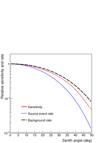
Figure 1.— Sensitivity in the detector field of view. Solid line: zenith angle dependence of the sensitivity to a Crab-like source. The sensitivity is normalized to a zenith angle $\theta$ = 0^∘. Dotted line: zenith angle dependence of the gamma ray event rate. Dashed line: zenith angle dependence of the background rate; both rates are normalized to $\theta$ = 0^∘.

One of the distinctive features of air shower arrays is the large field of view (FOV), in principle including the entire overhead sky. Gamma ray sources cross the FOV with different paths according to their declinations. The sensitivity is not uniform in the field of view. Given a photon flux, the atmospheric absorption reduces the rate of showers for increasing zenith angles. The cosmic ray background also decreases but more slowly, and the combination of the two rates determines the trend of the sensitivity as a function of the zenith angle. Fig.1 shows the event rate in ARGO-YBJ expected from a Crab-like source as a function of the zenith angle $\theta$, normalized to the rate at $\theta$ = 0^∘, compared to the background rate. In the same figure the dependence of the detector sensitivity on $\theta$ is also reported. According to simulations, the sensitivity at $\theta$ = 30^∘ (45^∘) is reduced by a factor $\sim$2 ($\sim$10) with respect to the sensitivity at $\theta$ = 0^∘.

The capability to detect a given source depends on its path in the field of view (determined by the source declination), and in particular on the amount of time that the source lies at different zenith angles. The maximum significance is for a declination $\delta_{max}$ = $\lambda$, where $\lambda$ = 30.1^∘ is the latitude of the detector. Given a Crab-like source, the sensitivity decreases by less than 10$\%$ for declinations $\lvert\delta$-$\delta_{max}\rvert<$10^∘, while it is reduced by a factor $\sim$2 for declinations $\lvert\delta$-$\delta_{max}\rvert\sim$30^∘. The declination dependence is slightly stronger (weaker) for sources with softer (harder) spectra with respect to the Crab Nebula (Bartoli et al.,, 2013).

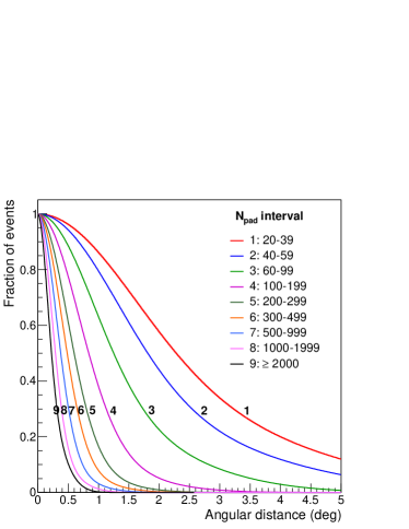
Figure 2.— Angular resolution for different N_pad intervals, according to simulations. The curves represent the fraction of events beyond the angular distance $d$ from the source, as a function of $d$.

At the ARGO-YBJ site, the Crab Nebula (declination $\delta$ = 22.01^∘) culminates at a zenith angle $\theta$ = 8.1^∘ and lies at zenith angles $\theta$ $<$ 45^∘ for 6.6 hours per sidereal day. In general, following a source for a longer time per day increases the signal significance, because of the increasing statistics, but since the signal to background ratio decreases at large zenith angles, there is a maximum zenith angle beyond which the significance begins to reduce. According to simulations, the maximum zenith angle for the Crab Nebula is $\sim$45^∘.

2.2. Angular Resolution

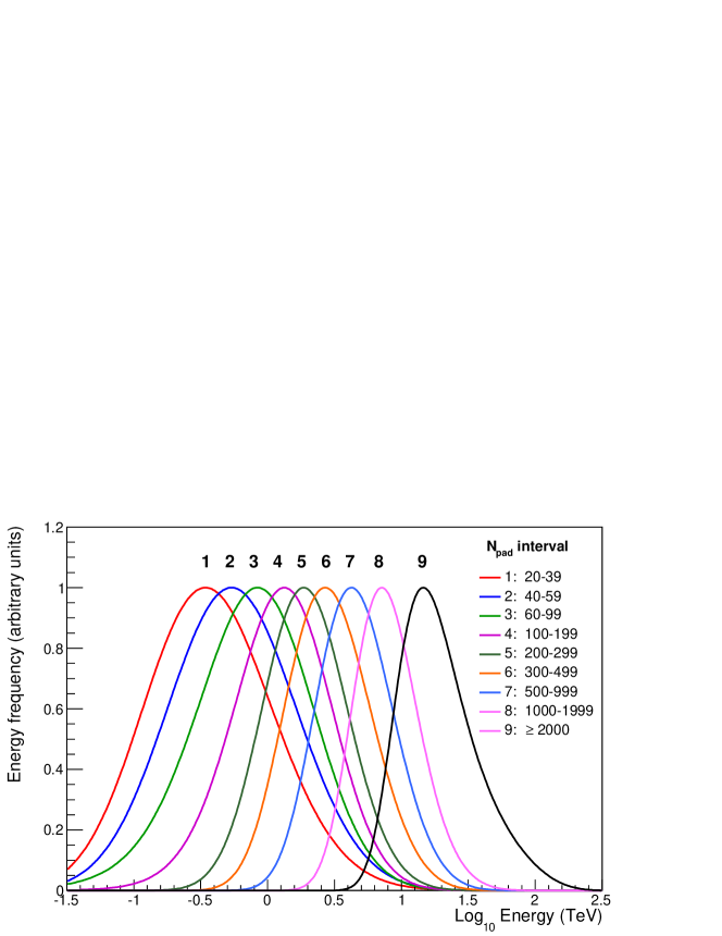
Figure 3.— Normalized distribution of the primary gamma ray energy for different N_pad intervals, for a Crab-like source.

The sensitivity needed to observe a gamma ray source is related to the angular resolution, which determines the amount of cosmic ray background. We evaluate the shower arrival direction by fitting the shower front with a conical shape centered on the shower core position, to take into account the time delay of secondary particles with respect to a flat front, a delay that increases with the distance from the core. We set this delay to 0.1 ns m^-1 (Aielli et al.,, 2009).

The high granularity of the detector allows the study of the shower profile in great detail and the accurate determination of the core position by fitting the lateral density distribution with a Nishimura-Kamata-Greisen-like function. According to simulations, the core position error depends on the number of hit pads N_pad and on the core distance from the detector center. For gamma ray induced showers with a core distance less than 50 m, the average core position error is less than 8 (2) m for N${}_{pad}\geq$ 100 (1000).

The point spread function (PSF) also depends on N_pad, and for a given N_pad value, it worsens as the shower core distance from the detector center increases. The angular resolution for showers induced by cosmic rays has been checked by studying the Moon shadow, observed by ARGO-YBJ with a statistical significance of $\sim$9 standard deviations per month. The shape of the shadow cast by the Moon on the cosmic ray flux provides a measurement of the detector PSF. This measurement has been found to be in excellent agreement with expectations, confirming the reliability of the simulation procedure (Bartoli et al., 2011b, ).

The PSF for gamma ray showers is narrower than the cosmic ray one by $\sim$30-40$\%$, due to the better defined time profile of the showers. To improve the angular resolution for gamma ray astronomy studies, quality cuts have been implemented, by rejecting the events with a core distance larger than a given value $D_{cut}$ (depending on N_pad) and with an average time spread of the particles with respect to the fitted shower front exceeding 9 ns (Bartoli et al.,, 2013). The values of $D_{cut}$ are given in Table 1. The fraction of gamma rays passing the selection cuts depends on N_pad averaging $\sim$80$\%$, whereas the fraction of surviving background events is $\sim$76$\%$ for N_pad $<$ 100 and $\sim$50$\%$ for N${}_{pad}\geq$ 100. The selection also acts as a mild gamma/hadron discrimination for events with N${}_{pad}\geq$ 100 (the sensitivity increases by a factor $\sim$1.1).

Table 1Characteristics of Crab Nebula simulated events.

Npad	$D_{cut}$	Core position	$R_{39}$	Median energy
	(m)	error (m)	(deg)	(TeV)
20-39	no limits	37	1.88	0.34
40-59	no limits	28	1.50	0.53
60-99	90	12	1.04	0.79
100-199	70	6.8	0.70	1.3
200-299	60	4.2	0.50	2.1
300-499	60	3.3	0.41	3.1
500-999	40	2.3	0.32	4.8
1000-1999	30	1.6	0.24	8.1
$\geq$ 2000	30	1.0	0.19	17.7

Note. —

^a Maximum distance of the shower core from the detector center beyond which the events are rejected.

^b Distance between the true and the reconstructed cores containing 68$\%$ of the events.

^c Angular resolution, defined as the 39$\%$ containment radius.

The arrival directions of the selected showers are also corrected for the systematic error due to the partial sampling of the shower front when the core is close to the edge of the detector (Eckmann,, 1991). This systematic error is related to the angle between the vector “shower core-detector center” and the shower arrival direction. For events with N${}_{pad}\geq$ 100, for which the core position is determined with more accuracy, the error can be considerably reduced.

These selections and corrections shrink the PSF by a factor ranging from $\sim$1.1 for events with N_pad = 20-39, up to $\sim$2, for N${}_{pad}\geq$ 1000. The PSFs obtained by simulating the Crab Nebula along its daily path up to $\theta$ = 45^∘ are shown in Fig.2 for different intervals of N_pad.

To describe the PSFs analitically, that for small values of N_pad cannot be simply fitted by a two-dimensional Gaussian function, the simulated distributions have been fitted with a linear combination of two Gaussians. In general, when the PSF is described by a single Gaussian (F($r$) = 1/(2$\pi$$\sigma^{2}$) $\exp$ (-$r^{2}$/$\sigma^{2}$), where $r$ is the angular distance from the source position), the value of the root mean square $\sigma$ is commonly defined as the “angular resolution”. In this case the fraction of events within 1 $\sigma$ is 39$\%$. For our PSFs, the value of the 39$\%$ containment radius $R_{39}$ ranges from 0.19^∘ for N${}_{pad}\geq$ 2000 to 1.9^∘ for N_pad = 20-39. Table 1 reports the values of $R_{39}$ for different N_pad intervals, together with the core position error, after quality cuts, as obtained by simulating the source during the daily path in the ARGO-YBJ field of view.

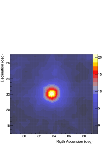
Figure 4.— Significance map of the Crab Nebula region, after smoothing and background subtraction.

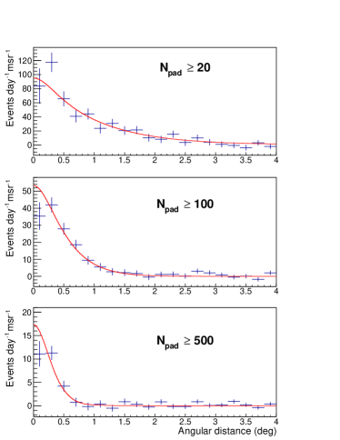
Figure 5.— Comparison of experimental and simulated PSFs: event rate per solid angle as a function of the angular distance from the source position, for events with N${}_{pad}\geq$ 20, 100 and 500. The solid lines are the results of the simulation.

2.3. Energy Measurement

The number of hit pads N_pad is the observable related to the primary energy that is used to infer the source spectrum. In general, the number of particles at ground level is not a very accurate estimator of the primary energy of the single event, due to the large fluctuations in the shower development in the atmosphere. Moreover, for a given shower, the number of particles detected in a finite area detector like ARGO-YBJ depends on the position of the shower core with respect to the detector center; for small showers this is especially poorly determined.

The relation between N_pad and the primary gamma ray energy of showers surviving the selection cuts is illustrated in Fig.3, where the corresponding primary energy distributions for different N_pad intervals are reported, as obtained by simulating a Crab-like source with a power law spectrum with index -2.63. The distributions are broad, with extended overlapping regions, spanning over more than one order of magnitude for small N_pad values. The median energies for different N_pad intervals are given in Table 1. They range from 340 GeV for events with N_pad = 20-39, to $\sim$18 TeV for N${}_{pad}\geq$ 2000.

Since the variable N_pad does not allow the accurate measurement of the primary energy of the single event, the energy spectrum is evaluated by studying the global distribution of N_pad. The observed distribution is compared to a set of simulated ones obtained with different test spectra, to determine the spectrum that better reproduces the data.

3. The Crab Nebula Signal

The data set used for this analysis contains all the events recorded from 2007 November to 2013 February, with N${}_{pad}\geq$ 20. The total on-source time is 1.12 $\times$ 10⁴ hours.

For each source transit, the events are used to fill a set of nine 12${}^{\circ}\times$12^∘ sky maps centered on the Crab Nebula position, with a bin size of 0.1${}^{\circ}\times$0.1^∘ in right ascension and declination (“event maps”). Each map corresponds to a defined N_pad interval: 20-39, 40-59, 60-99, 100-199, 200-299, 300-499, 500-999, 1000-1999 and N${}_{pad}\geq$ 2000.

To extract the excess of gamma rays, the cosmic ray background has to be estimated and subtracted. Using the time swapping method (Alexandreas et al.,, 1993), the shower data recorded in a time interval $\Delta t$ = 2-3 hours are used to evaluate the “background maps”, i.e. the expected number of cosmic ray events in any location of the map for the given time interval. This method assumes that during the interval $\Delta t$ the shape of the distribution of the arrival directions of cosmic rays in local coordinates does not change, while the overall rate could change due to atmospheric and detector effects. The value of the time interval $\Delta$t is less than a few hours to minimize the systematic effects due to the environmental parameters variations that could change the distribution of the arrival directions.

The time swapping method is a sort of “simulation” based on real data: for each detected event, $n_{f}$ ”fake” events (with $n_{f}$ = 10) are generated by replacing the original arrival time with new ones, randomly selected from an event buffer that spans the time $\Delta$t of data taking. By changing the time, the fake events maintain the same declination of the original event, but have a different right ascension. With these events a new sky map (background map) is built, with a statistics $n_{f}$ times larger than the event map in order to reduce the fluctuations. To avoid the inclusion of the source events in the background evaluation, the showers inside a circular region around the source (with a radius related to the PSF and depending on N_pad) are excluded from the time swapping procedure. A correction on the number of swaps is applied to take into account the rejected events in the source region (Fleysher et al.,, 2004).

Event and background maps are then smoothed according to the PSF corresponding to each N_pad interval. Finally, the smoothed background maps are subtracted to the smoothed event maps, obtaining the “excess maps”, where for every bin the statistical significance of the excess is calculated as:

$$n_{\sigma}=\frac{N_{E}-N_{B}}{\sqrt{\delta N_{E}^{2}+\delta N_{B}^{2}}}$$

with $N_{E}$ = $\Sigma_{i}$ $n_{i}$ $w_{i}$ and $N_{B}$ = $\Sigma_{i}$ $b_{i}$ $w_{i}$ / $n_{f}$. In these expressions $n_{i}$ and $b_{i}$ are the number of events of the i^th bin of the event map and background map, respectively, $w_{i}$ is a normalized weight, proportional to the value of the PSF at the angular distance of the i^th bin, and $n_{f}$ is the number of swappings. The sum is over all the bins inside a radius $R_{max}$, chosen to contain the signal events and depending on the PSF. Since the number of events per bin is large, the fluctuations follow the Gaussian statistics, hence the errors on $N_{E}$ and $N_{B}$ are: $\delta N_{E}$ = $\sqrt{\Sigma_{i}n_{i}w_{i}^{2}}$ and $\delta N_{B}$ = $\sqrt{\Sigma_{i}b_{i}w_{i}^{2}/n_{f}^{2}}$.

The number of gamma ray events from the source is:

$$N_{\gamma}=\frac{N_{E}-N_{B}}{2\pi\int_{0}^{R_{max}}w(r)^{2}rdr}$$

where $w(r)$ is the weight used in the smoothing procedure calculated at the angular distance $r$ from the source position.

When adding all data, an excess consistent with the Crab Nebula position is observed in each of the 9 maps, with a total statistical significance of 21.1 standard deviations.

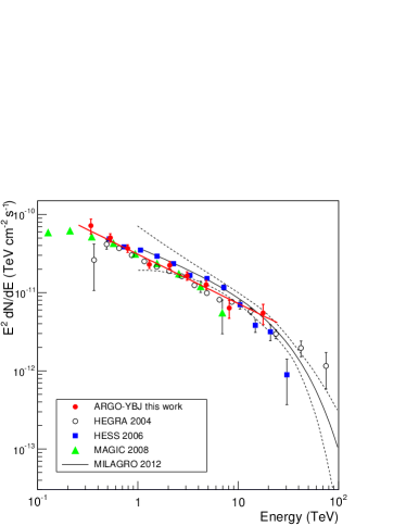
Figure 6.— Crab Nebula differential energy spectrum multiplied by E² measured by ARGO-YBJ and other experiments. The thick solid line (red in the online version) represents the best fit of the ARGO-YBJ data. The dotted lines delimit the 1 sigma error band of the Milagro spectrum.

The number of excess events are $\sim$3.3 $\times$ 10⁵, corresponding to 189 $\pm$ 16 day^-1, where a “day” means a source transit. Table 2 gives the signal significance for each map and the corresponding event rates measured from the source. For comparison the background rates measured inside an angular window of 1^∘ radius around the source are given. Fig. 4 shows the total significance map.

Finally, the gamma ray signal can be used to check the detector angular resolution since the Crab Nebula angular size is small compared to the detector PSF. Fig. 5 shows the distribution of the arrival directions of the excess showers with respect to the source position, for N${}_{pad}\geq$ 20, 100 and 500, compared to simulations. The agreement is excellent.

Table 2Summary of Crab Nebula data.

Npad	Photon rate	Background rate	Significance	Emed	Differential flux
	(events day-1)	(events day-1)	(s.d.)	(TeV)	(ph cm-2 s-1 TeV-1)
20-39	56.7 $\pm$ 12.2	1.3$\times$104	4.6	0.34	(6.23 $\pm$ 1.34)$\times$10-10
40-59	75.4 $\pm$ 9.2	1.1$\times$104	8.2	0.53	(1.80 $\pm$ 0.21)$\times$10-10
60-99	34.7 $\pm$ 3.9	4.2$\times$103	9.0	0.79	(5.92 $\pm$ 0.66)$\times$10-11
100-199	15.4 $\pm$ 1.7	1.9$\times$103	8.9	1.30	(1.37 $\pm$ 0.15)$\times$10-11
200-299	5.23 $\pm$ 0.61	4.9$\times$102	8.5	2.1	(5.30 $\pm$ 0.63)$\times$10-12
300-499	3.51 $\pm$ 0.44	3.8$\times$102	8.0	3.1	(1.75 $\pm$ 0.22)$\times$10-12
500-999	2.07 $\pm$ 0.27	2.4$\times$102	7.6	4.8	(5.62 $\pm$ 0.74)$\times$10-13
1000-1999	0.50 $\pm$ 0.13	87.4	3.8	8.1	(1.00 $\pm$ 0.26)$\times$10-13
$\geq$ 2000	0.23 $\pm$ 0.07	34.2	3.5	17.7	(1.87 $\pm$ 0.54)$\times$10-14

Note. —

^a Average background rate within an angular distance of 1^∘ from the source.

4. Energy Spectrum

The energy spectrum is evaluated by comparing the number of events detected from the Crab Nebula in the previously defined N_pad intervals to the expected number given by a simulation assuming a set of test spectra. We consider the power law spectrum:

$$\frac{dN}{dE}(I_{0},\alpha)=I_{0}\biggl{(}\frac{E}{2\;\mathrm{TeV}}\biggr{)}^{-\alpha},$$

where the flux normalization I₀ and slope $\alpha$ are the parameters to be estimated with the fitting procedure.

The fit is made by minimizing the value of $\chi^{2}$, evaluated for any couple of parameters as:

$$\chi^{2}(I_{0},\alpha)=\sum_{j=1,9}\frac{(N^{j}_{\gamma}-N^{j}_{MC}(I_{0},\alpha))^{2}}{(\delta N^{j}_{\gamma})^{2}+(\delta N^{j}_{MC})^{2}}$$

where $N^{j}_{\gamma}$ and $N^{j}_{MC}$ are the number of events detected and expected, respectively, in the $j^{th}$ N_pad interval.

The obtained best-fit parameters are $I_{0}$ = (5.2 $\pm$ 0.2) $\times$ 10^-12 photons cm^-2 s^-1 TeV^-1, and $\alpha$ = -2.63 $\pm$ 0.05, with $\chi^{2}$ = 5.8 for 7 degrees of freedom, corresponding to a p-value $p$ = 0.56. The integral flux above 1 TeV is 1.97 $\times$ 10^-11 photons cm^-2 s^-1. The flux at 1 TeV obtained in this work is 7$\%$ higher than that reported in a previous ARGO-YBJ paper (Bartoli et al.,, 2013). The difference is due to the correction of the event rates applied in this work, to reduce environmental and detector effects on the trigger rate, as described in Section 5.3.

Fig. 6 shows the obtained spectrum compared with the results of other experiments. The energy of each point is the gamma ray median energy for the corresponding N_pad interval. The values of energies and differential fluxes are given in Table 2. The spectrum is consistent with a constant slope from $\sim$300 GeV to $\sim$20 TeV and agrees rather well with the measurement by HEGRA and MAGIC, whereas the HESS and Milagro fluxes are about 20$\%$ higher in the $\sim$1-10 TeV energy range.

The data are less clear concerning a possible energy cutoff at higher energies. MAGIC (Albert et al.,, 2008) and HESS (Aharonian et al.,, 2006) show a steepening below 20 TeV, while the HEGRA spectrum is harder and continues with a slight softening up to $\sim$75 TeV (Aharonian et al.,, 2004). A possible cutoff is also observed by Milagro at $\sim$30 TeV (Abdo et al.,, 2012). The limited statistics of our data at high energy does not allow to draw any conclusion about the spectral properties above 20 TeV. Selecting events with N${}_{pad}\geq$ 3000 (whose median energy is 26 TeV assuming a power law spectrum with index $\alpha$ = -2.63) the statistical significance of the signal is 0.75.

When fitting the data with a power law spectrum with an exponential cutoff:

$$\frac{dN}{dE}(I_{0},\alpha,E_{cut})=I_{0}\biggl{(}\frac{E}{2\;\mathrm{TeV}}\biggr{)}^{-\alpha}\;\exp\;(-E/E_{cut})$$

the obtained p-value is always smaller than without a cutoff, for any value of $E_{cut}$. For E_cut = 14.3 TeV (the best-fit value obtained by HESS) the p-value is 0.13. We found that the p-value is larger than 10$\%$ for any value of E_cut $>$ 12 TeV, indicating that the presence of a cutoff above $\sim$10 TeV cannot be excluded even if our data seems more consistent with a pure power law.

4.1. Estimation of Systematic Errors

The previous results can be affected by systematic errors of different origin. In the following we discuss the possible sources of systematics, evaluating their effects both on the flux normalization and the spectral slope.

1) Energy scale. In our measurement the number of hit pads N_pad is used as an estimator of the primary energy. The relation between the primary energy and N_pad is given by Monte Carlo simulations. Possible uncertainties and simplifications in the simulation procedure (both in the shower development and the detector response) could produce an incorrect N_pad value and consequently an error in the energy scale.

The energy scale reliability has been checked using the Moon shadow. Due to the geomagnetic field, cosmic rays are deflected according to their energy and the shadow that the Moon casts on the cosmic ray flux is shifted with respect to the Moon position by an amount depending on the energy. The westward shift of the shadow has been measured for different N_pad intervals and compared to simulations. From the analysis of the Moon data, we found that the total absolute energy scale error is less than 13$\%$ in the proton energy range $\sim$1-30 TeV (Bartoli et al., 2011b, ). This estimate includes the uncertainties of the cosmic ray elemental composition and the hadronic interaction model.

From this result, given a gamma ray spectrum with index $\alpha$ = -2.63, the corresponding systematic error in the flux normalization would be less than 22$\%$.

2) Pointing error. Fitting the angular distribution of gamma rays around the Crab Nebula position we found that the pointing error is less than 0.1^∘. A pointing error affects the measured gamma ray flux, since the number of photons is obtained by a smoothing procedure weighting the events with a PSF centered at the source nominal position. An incorrect position would produce a loss of signal. Since the PSF is narrower for events with large N_pad, the loss is larger at high multiplicities, and generates a steepening of the spectrum. According to our simulation, a pointing error of 0.1^∘ would produce a loss of signal ranging from 0.1$\%$ for N_pad = 20-39 to 6.0$\%$ for N${}_{pad}>$2000. As a consequence, the spectral index would increase by 0.01 and the flux normalization would decrease by 2$\%$.

3) Background evaluation. Our measurement is based on a very precise evaluation of the background. As explained in Section 3, the number of gamma rays is given by the difference between the number of events detected in the event map (that contains the source events plus the cosmic ray background) and the number of background events estimated with the time swapping method. Since the ratio between the number of gamma rays and the number of background events is very small (ranging from $\sim$3 $\times$ 10^-4 for N_pad = 20-39 up to $\sim$4 $\times$ 10^-2 for N_pad $>$ 300), even a small systematic error in the background evaluation could produce a big error in the source flux.

Possible sources of systematics are: a) the presence of cosmic ray excess regions due to the medium scale anisotropy, as those reported in (Bartoli et al., 2013c, ), close to the source, b) changes in atmospheric conditions able to modify the background distribution in local coordinates in less than 2-3 hours, and c) the detector malfunctioning.

Such effects, when present, could generate extended regions in the signal map with evident excesses or deficits, in some cases involving the whole map. Instead, an accurate evaluation of the background produces a map with all the bin contents consistent with zero except at the position of real sources.

Concerning the medium scale anisotropy, we adopted a particular procedure to correct the background systematics in the sky regions coincident or adjacent to cosmic ray excesses (Bartoli et al.,, 2013). This correction is not necessary in the Crab Nebula region.

Concerning points $b$ and $c$, it has to be specified that the maps are built with data sets of 2-3 hours and individually checked. When a map shows significant anomalies, the corresponding dataset is rejected, so only “good maps” are combined to build to the “total maps”.

To test the background reliability of the total maps, we use the regions that are not involved in the Crab Nebula emission, i.e., the bins with an angular distance from the source larger than a minimum value, depending on the PSF. From these “out-source” regions we expect no significant excess, since they do not include any other known gamma ray source with a flux above the ARGO-YBJ sensitivity. For any of the nine maps we have evaluated the distribution of the excesses in the out-source region bins (before smoothing). We found that all the distributions are well described by Gauss functions with mean values consistent with zero and r.m.s. consistent with unit.

Adding all the nine maps together, the total number of events detected from the out-source regions is 1.18 $\times$ 10⁹. This value differs from the corresponding estimated background by -9.3 $\times$ 10³ events, corresponding to -0.3 standard deviations. Since there is no significant excess or deficit of events, we can calculate the upper limit of the systematic error in the out-source region. We found that the relative error in the background value is less than 3.7 $\times$ 10^-5 at 90$\%$ confidence level.

We can reasonably assume that a similar systematic error involves the region of the map containing the source signal, and that all the nine maps have comparable systematic errors. Based on these assumptions, we can evaluate the effects of such an error on the signal, which are obviously more relevant for the maps in which the signal-to-background ratio is smaller. We found that the error in the photon number is $<$13$\%$ for N_pad = 20-39, $<$1$\%$ for N_pad = 100-199, and $<$0.01$\%$ for N_pad $\geq$ 1000.

According to these values, the corresponding systematic error in the spectrum flux normalization would be less than 2$\%$, and the error in the spectral index would be less than 0.05.

4) Event rate variations. Studying the rate of cosmic ray showers over five years, we observed variations on timescales from hours to months up to 10$\%$ with respect to the mean value. These variations are mostly due to: a) variation of atmospheric pressure and temperature that modify the showers propagation in the atmosphere, b) variation of the detector efficiency due to changes of the local temperature and pressure, c) aging of the detector.

Gamma rays are assumed to be subject to similar variations. To study the stability of the Crab Nebula flux, we corrected the rate of the events observed from the source using the cosmic ray rate as a normalization factor (see Section 5.3). However, an absolute normalization cannot be performed. The Monte carlo simulations refer to a fixed atmospheric condition and a given detection efficiency, that cannot exactly reproduce the average effect over several years of different conditions. Considering the amount of the observed rate variation, a reasonable estimation indicates a possible systematic error in the flux smaller than 4$\%$.

Total systematic error. Adding all these contributions linearly, we conservatively estimate the total systematic error to be less than 30$\%$ for the flux normalization and 0.06 for the spectral index.

5. Crab Nebula Light Curve

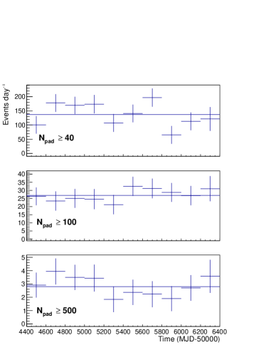
Figure 7.— Rate of events detected from the Crab Nebula for different N_pad thresholds as a function of time. The bin width is 200 days. The lines represent the average values.

To study the stability of the Crab Nebula emission, we consider the events with N${}_{pad}\geq$ 40. Our total dataset consists of 1851 days, with an average observation time of 6.0 hours per day. The average rate of events with N${}_{pad}\geq$ 40 is 137 $\pm$ 10 day^-1.

Figure 7 shows the observed rate for events with N${}_{pad}\geq$ 40, 100 and 500, as a function of the Julian date, in bins of 200 days. The median energies corresponding to these N_pad thresholds are 0.76, 1.8 and 5.1 TeV, respectively. The signal appears stable during five years for any threshold within the statistical fluctuations. Assuming a constant rate, the obtained $\chi^{2}$ are 15.7, 3.27 and 5.17 (with 9 d.o.f.) for N${}_{pad}\geq$ 40, 100 and 500. The corresponding p-values are 0.073, 0.95 and 0.82, respectively.

A six-year monitoring of the Crab Nebula was previously performed by the Tibet-III air shower array from 1999 to 2005, at energies $\sim$3 TeV, with a sensitivity 3-4 times lower than that of ARGO-YBJ, reporting a yearly flux consistent with a steady emission (Amenomori et al.,, 2009).

5.1. Search for Flares

To make a “blind” search for short time rate variations, we consider all the time intervals of duration $\Delta t$ ranging from 1 to 15 days, starting from every observation day. This time range has been chosen on the basis of the duration of the flares observed in the GeV energy region. For each interval we compare the observed rate of Crab events with the average rate and evaluate the significance of the excess as: $\sigma_{i}$ = ($R_{i}-R_{m}$) / $\delta(R_{i}-R_{m})$, where $R_{i}$ is the counting rate in the i-th interval, $R_{m}$ is the average counting rate, and $\delta(R_{i}-R_{m})$ is the statistical error of the difference $R_{i}-R_{m}$. Note that the values of $\sigma_{i}$ are not independent, since the time intervals overlap.

Fig. 8 shows the distributions of $\sigma_{i}$ for $\Delta t$ = 1 day and $\Delta t$ = 2-15 days, for N${}_{pad}\geq$ 40. The total number of intervals is 1851 for $\Delta t$ = 1 and 25911 for $\Delta t$ = 2-15 days. The distributions can be fitted by a Gauss function with mean value $m$ = -0.04 $\pm$ 0.03 and r.m.s.= 1.05 $\pm$ 0.02 for $\Delta t$ = 1 day, and $m$ = -0.06 $\pm$ 0.01 and r.m.s.= 1.061 $\pm$ 0.005 for $\Delta t$ = 2-15 days. The root mean square values indicate rate variations slightly larger than what expected by statistical fluctuations. However, no significant excess is observed for any of the considered time intervals.

Given the ARGO-YBJ sensitivity, a flare would produce a 5 s.d. signal (pre-trial) if the flux exceeds the average value by a factor $f$ $\sim$ 10 / $\sqrt{\Delta t(\mathrm{days})}$.

5.2. Correlation with Fermi-LAT Data

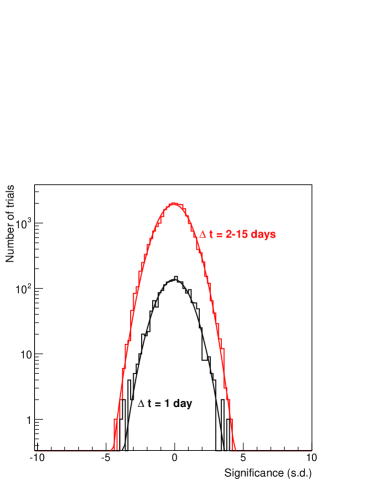
Figure 8.— Search for flares: distribution of the excesses from the Crab Nebula around the average value, in units of standard deviations, for different flare durations $\Delta t$.

To reduce the number of trials in the search for possible flares, we can limit our analysis to the days in which a flare was observed by satellite instruments at lower energies. We consider the Fermi-LAT daily light curve at energy E $>$ 100 MeV from 2008 August to 2013 February, obtained through the analysis of the scientific Fermi data publicly available at the Fermi Science Support Center.

The first panel of Figure 9 shows the daily light curve, representing the sum of the nebula and pulsar fluxes. The average flux is (2.66 $\pm$ 0.01) $\times$ 10^-6 photons cm^-2 s^-1. Also excluding the days with flares, the rate is variable, with modulations on timescales of weeks and months.

Table 3ARGO-YBJ results during the three largest Crab Nebula flares observed by Fermi-LAT.

	$\Delta$t	Max.Fermi flux	ARGO-YBJ	ARGO rate	ARGO rate	ARGO rate
	(days)	(ph cm-2 s-1)	Observation	N${}_{pad}\geq$40	N${}_{pad}\geq$100	N${}_{pad}\geq$500
			time (hr)	(ph day-1)	(ph day-1)	(ph day-1)
Flare 1	8	6.3$\pm$0.8$\times$10-6	49.6	142 $\pm$ 151	21 $\pm$ 28	2.5 $\pm$ 4.6
Flare 2	5	6.4$\pm$0.8$\times$10-6	31.5	265 $\pm$ 190	58 $\pm$ 36	-3.8 $\pm$ 5.7
Flare 3	9	19.8$\pm$0.8$\times$10-6	58.0	228 $\pm$ 144	51 $\pm$ 27	2.9 $\pm$ 4.4
Sum of 3 flares	22		139	205 $\pm$ 91	41 $\pm$ 17	1.3 $\pm$ 2.8
All ARGO data				137 $\pm$ 10	27 $\pm$ 2	2.8 $\pm$ 0.3

Note. —

^a Start time MJD 54864 (2009 February 02)

^b Start time MJD 55457 (2010 September 18)

^c Start time MJD 55662 (2011 April 11)

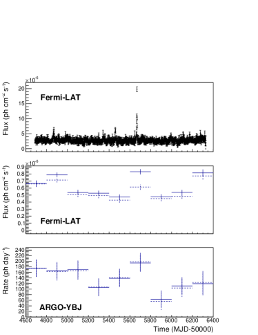
Figure 9.— Panel 1: daily light curve of the Crab Nebula and pulsar by Fermi-LAT; Panel 2: light curve of the Crab Nebula (pulsar subtracted) in bins of 200 days, by Fermi-LAT; Panel 3: light curve of the Crab Nebula by ARGO-YBJ for events with N${}_{pad}\geq$ 40. The dashed line in panels 2 and 3 has been obtained excluding the days with flares.

First we consider the three largest Fermi flares, which occurred in 2009 February, 2010 September and 2011 April (Abdo et al.,, 2011; Buehler et al.,, 2012). To define the time boundaries and the duration of these flares we select the days in which the Fermi flux is higher than 4 $\times$ 10^-6 photons cm^-2 s^-1. The dates and the duration of the three flares are given in Table 3. The counting rates from the Crab Nebula measured by ARGO-YBJ with events with N${}_{pad}\geq$ 40 during the flares are compared with the average rate of 137 $\pm$ 10 day^-1. In all cases, the rates are slightly higher than the average value, but consistent with it within statistical errors (see Table 3). Summing the three flares the average rate is 205 $\pm$ 91 day^-1. Table 3 also shows the results concerning the events with N${}_{pad}\geq$ 100 and 500. No significant excess is present in this case, either.

Our preliminary analysis reported in (Aielli et al.,, 2010) showed a 4 standard deviations excess observed in the time interval from 2010 September 17 to 22 from a direction consistent with the Crab Nebula. However, removing the contribution of the steady flux and taking into account the number of trials, the post-trial significance was about two standard deviations. A further excess with a similar post-trial statistical significance was observed during the 2011 April flare (Vernetto,, 2013). In the present work, based on a better shower reconstruction and the event selection described in Section 2.2, the significance of the Crab Nebula signal integrated over 5 years increases by about 15$\%$ with respect to the old analysis, but the signal observed during the Fermi flares decreases. The flux measured during the flares appears slightly higher than what would be expected from the steady emission, but consistent with it within one standard deviation. Both our previous analysis and the current one hint at a possible flux enhancement during the flares, but the reduced significance prevents us from drawing a definitive conclusion.

To extend the search for flares to the whole observation time, and not limit the analysis to the largest flares, we selected the Fermi data according to the measured daily flux and checked the corresponding ARGO-YBJ event rate. Table 4 reports the ARGO-YBJ rates for different levels of the Fermi flux and different N_pad thresholds. The rates are consistent with the average rate for any Fermi flux level. In particular, the ARGO-YBJ rate (for N${}_{pad}\geq$ 40) measured in the 62 days in which the Fermi flux exceeds 4 $\times$ 10^-6 ph cm^-2 s^-1, is 190 $\pm$ 55 day^-1 i.e. 1.4 $\pm$ 0.4 times higher than the average rate.

Table 4ARGO-YBJ photon rate for different flux levels measured by Fermi.

Fermi flux	Number of days	ARGO rate	ARGO rate	ARGO rate
( 10-6 ph cm-2 s-1)		N${}_{pad}\geq$40	N${}_{pad}\geq$100	N${}_{pad}\geq$500
		(ph day-1)	(ph day-1)	(ph day-1)
$<$ 2.0	175	197 $\pm$ 34	26 $\pm$ 6	3.1 $\pm$ 1.0
2.0-3.0	915	118 $\pm$ 15	27 $\pm$ 3	2.8 $\pm$ 0.4
3.0-4.0	435	148 $\pm$ 21	28 $\pm$ 4	3.0 $\pm$ 4.3
4.0-5.0	46	188 $\pm$ 64	33 $\pm$ 12	1.9 $\pm$ 2.0
$>$ 5.0	16	198 $\pm$ 107	54 $\pm$ 20	0.2 $\pm$ 3.2
All ARGO data		137 $\pm$ 10	27 $\pm$ 2	2.8 $\pm$ 0.3

Finally, to study a possible correlation on timescales of months or years, we compare the light curves of the two detectors over the common observing time ($\sim$ 4.5 years), dividing the data into bins of 200 days. The bin width is chosen in order to have a significant signal in the ARGO-YBJ data (about 7 s.d.).

Since the flux measured by Fermi is the sum of the nebula and pulsar contributions, and since the pulsar flux $F_{P}$ averaged over the pulsation period is also stable during flares ($F_{P}$ = (2.04 $\pm$ 0.01) $\times$ 10^-6 photons cm^-2 s^-1 for E $>$100 MeV (Buehler et al.,, 2012)), the flux of the pulsar has been subtracted. The obtained average nebula flux is (6.2 $\pm$ 0.1) $\times$ 10^-7 photons cm^-2 s^-1. The nebula flux shows variations up to $\sim$30$\%$ of the average flux, with $\chi^{2}$ = 126, for 8 d.o.f. (see the second panel of Fig. 9). The large variations are not only due to flares. In the same figure the dashed curve shows the flux obtained excluding the 62 “flaring days”. In this case the average value is (5.6 $\pm$ 0.1) $\times$ 10^-7 photons cm^-2 s^-1, with $\chi^{2}$ = 80.

The lower panel of Fig. 9 shows the corresponding ARGO-YBJ data for N${}_{pad}\geq$ 40. The average rate is 139.3 $\pm$ 10.6 events day^-1 ($\chi^{2}$ = 14.2 for 8 d.o.f., p-value $p$ = 0.077). Even if the ARGO-YBJ rate variations are consistent with statistical fluctuations, the Fermi and ARGO-YBJ data seems to follow a similar trend. The ARGO-YBJ rate appears higher in the “hot” Fermi periods. The dashed curve is obtained after the exclusion of the flaring days.

Fig. 10 shows the ARGO-YBJ percentage rate variation with respect to the mean value ($\Delta F_{ARGO}$) as a function of the corresponding variation of the Fermi rate ($\Delta F_{Fermi}$), for the 9 bins of the light curve. The Pearson correlation coefficient between the two data sets is $r$ = 0.56 $\pm$ 0.22. The quoted error for $r$ is the root mean square of the distribution of the correlation coefficients obtained by simulating the fluctuations of the counting rates of each bin, according to their statistical errors. Fitting the 9 points with the function $\Delta F_{ARGO}$ = $a$ $\Delta F_{Fermi}$ + $b$, the values of the best-fit parameters are $a$ = 0.88 $\pm$ 0.37 and $b$ = 0.018 $\pm$ 0.079, with $\chi^{2}$ = 8.3 for 7 d.o.f. Discarding the 62 “flaring” days the correlation coefficient becomes $r$ = 0.45 $\pm$ 0.23 and the parameters of the linear fit are $a$ = 0.96 $\pm$ 0.45 and $b$ = 0.018 $\pm$ 0.082, with $\chi^{2}$ = 10.4.

The same analysis has been performed using a different bin width, ranging from 10 to 450 days. The corresponding correlation coefficient steadily increases from $r$ = 0.10 $\pm$ 0.06 (10 days) to $r$ = 0.59 $\pm$ 0.23 (450 days). It has to be noted, however, that when using a small bin width, the ARGO-YBJ signal is not significant enough to search for a correlation unless the flux variations are very large. In 10 days, for example, the average ARGO-YBJ signal is 137 $\pm$ 135 events day^-1. The statistical fluctuations would hide a possible flux variation, unless the flux becomes more than a factor of 4-5 higher than the average.

The above results refer to events with N${}_{pad}\geq$ 40. The correlation coefficient is lower when selecting more energetic events: using a bin width of 200 days, for N${}_{pad}\geq$ 100, $r$ = 0.19 $\pm$ 0.31; and for N${}_{pad}\geq$ 500, $r$ = 0.46 $\pm$ 0.28.

5.3. Stability of the ARGO-YBJ Data

When studying the time evolution of a signal over several years, a discussion on the possible causes of detector instabilities is mandatory, to exclude systematic effects that could produce artificial rate variations. Since the measured number of events from the source $N_{S}=N_{E}-N_{B}$ is the difference between the number of events $N_{E}$ detected in the source map and the number of background events $N_{B}$ estimated with the time swapping method, one must separately analyze the stability of the different contributions.

1) A loss of signal events $N_{S}$ could be produced by variations of the pointing accuracy. Studying the Moon shadow month by month, we have verified that the pointing is stable within 0.1 deg (Bartoli et al., 2011b, ). Given the moderate angular resolution for events with N${}_{pad}\geq$ 40, such a value could produce signal fluctuations of less than 2$\%$.

2) A worsening of the detector angular resolution (due to an increase of the time resolution of RPCs occurring at particularly low temperatures) could produce a loss of signal events $N_{S}$. A broadening of the PSF would also cause a decrease of the Moon shadow signal. That, however, is found to be stable within statistical fluctuations.

3) Atmospheric pressure and temperature variations can affect the RPC detection efficiency, which can also be altered by some RPC not working properly or by aging effects.

4) Pressure and temperature produce changes in the shower rate of the order of a few percent due to the different conditions in which the showers propagate in the atmosphere.

The two latter effects modify $N_{S}$, $N_{E}$ and $N_{B}$ by about the same factor (neglecting the different behavior of cosmic ray and gamma ray showers, that in this contest can be considered a second-order effect). This allows the use of $N_{B}$ to correct the Crab rate, multiplying the Crab rate observed in a given time interval by the correction factor $f_{c}$ = $B_{m}$/$B$, where $B_{m}$ is the average background rate and $B$ is the background rate in that interval. The light curve in Figure 7 has been corrected according to this method, with $f_{c}$ ranging from 0.91 to 1.07.

5) Further possible systematics could be an incorrect evaluation of the background $N_{B}$. In Section 4 we evaluated the accuracy of the background for the total source signal. To check the accuracy of the background along the years, we can use the same out-source regions previously defined. For events with N${}_{pad}\geq$ 40, the out-source light curve in 200-day bins has a mean value of -7.9 $\pm$ 19.0 events day^-1 and a $\chi^{2}$ = 10.2 for 9 d.o.f., corresponding to a p-value $p$ = 0.67. According to these results the background is stable and should not introduce any systematic effect on the rate of the Crab signal.

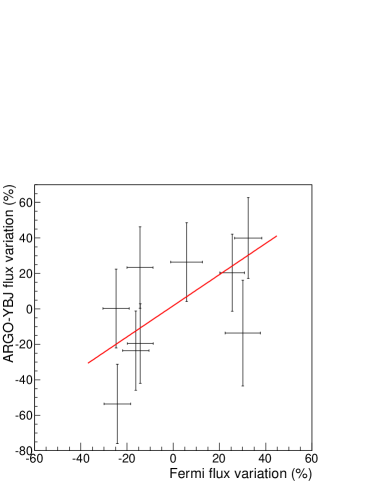
Figure 10.— Percentage variation of the Crab Nebula flux with respect to the average value: ARGO-YBJ vs Fermi-LAT data. The straight line is the best fit curve.

6. Summary and Conclusions

The ARGO-YBJ events recorded over five years have been analyzed to evaluate the Crab Nebula spectrum and study the temporal behavior of the gamma ray emission. Using the events with N${}_{pad}\geq$ 20, the statistical significance of the gamma ray signal reaches more than 21 standard deviations, and the observed photon rate is 189 $\pm$ 16 day^-1. The event angular distributions around the source are well described by the PSFs obtained by simulations.

The source spectrum extends over nearly 2 decades in energy and five decades in flux. The spectral shape is consistent with a power law behavior in the range 0.3-20 TeV with a spectral index -2.63 $\pm$ 0.05. An exponential cutoff would be consistent with our data in case of a cutoff energy higher than 12 TeV at 90$\%$ confidence level.

The study of the Crab Nebula light curve has been carried out to check the stability of the flux over years and to search for possible flares on the timescale of days. All the known sources of rate instabilities have been examined and the effects corrected.

Concerning flares, a blind search for flux increases of duration between 1 and 15 days shows no significant excess. The average rate of events with N${}_{pad}\geq$ 40 measured by ARGO-YBJ during the three most powerful flares detected by Fermi-LAT (in 2009 February, 2010 September and 2011 April) is 205 $\pm$ 91 day^-1, which is consistent with the average value of 137 $\pm$ 10 day^-1.

The five year ARGO-YBJ light curve with a binning of 200 days is consistent with a constant flux with a probability of 0.07. A correlation analysis with the corresponding Fermi-LAT data gives a Pearson correlation coefficient $r$ = 0.56 $\pm$ 0.22. The small statistical significance of these results does not allow the claim for a flux variability correlated with the observations at lower energies. If such a correlation was due to a real astrophysical phenomenon, the found regression coefficient $a$ = 0.88 $\pm$ 0.37 would imply a similar percentage variation in Fermi and ARGO-YBJ rates, suggesting a similar behavior of the gamma ray emission at energies $\sim$ 100 MeV and $\sim$1 TeV.

So far, no variation of the Crab Nebula flux at TeV energies has been reported by any detector. Assuming the flares observed by AGILE and Fermi due to synchrotron radiation from a population of electrons accelerated up to 10¹⁵ eV, the Inverse Compton emission associated with this population would occur in the Klein-Nishina regime and would produce gamma rays of energy approximately equal to that of the electrons. Such a flux would not be detectable by any of the existing gamma ray experiments. With these assumptions, a TeV excess could hardly be intepreted as IC emission associated with the synchrotron radiation observed at lower energies, and would require a completely new interpretation.

References

- Abdo et al., (2011) Abdo, A.A., Ackermann, M., Ajello, M., et al. 2011, Science 331, 739
- Abdo et al., (2012) Abdo, A.A., Allen, B.T., Atkins, R., et al. 2012, ApJ 750, 63
- Abramowski et al., (2013) Abramowski, A., Aharonian, F., Ait Benkhali, F., et al. 2014, A&A, 562, L4
- Aharonian et al., (2004) Aharonian, F.A., Akhperjanian, A., Beilicke, M., et al 2004, ApJ, 614, 897
- Aharonian et al., (2006) Aharonian, F.A., Akhperjanian, A.G., Bazer-Bachi, A.R., et al., 2006, A&A, 457, 899
- Aielli et al., (2006) Aielli, G., Assiro, R., Bacci, C., et al. 2006, Nucl. Instrum. Methods Phys. Res. A, 562, 92
- Aielli et al., (2008) Aielli, G., Bacci, C., Barone, F., et al. 2008, Astrop. Phys., 30, 85
- Aielli et al., (2009) Aielli, G., Bacci, C., Bartoli, B., et al. 2009, Astrop. Phys., 30, 287
- (9) Aielli, G., Bacci, C., Bartoli, B., et al. 2010b, ApJ, 714, L208
- Aielli et al., (2012) Aielli, G., Bacci, C., Bartoli, B., et al. 2012, Nucl. Instrum. Methods Phys. Res. A, 661, S56
- Aielli et al., (2010) Aielli, G., Camarri, P., Iuppa, R., et al. 2010, Astron. Telegram n.2921
- Albert et al., (2008) Albert, J., Aliu, E., Anderhub, H., et al. 2008, ApJ, 674, 1037
- Alexandreas et al., (1993) Alexandreas, D.E., Berley, D., Biller, S., et al. 1993, Nucl. Instrum. Methods Phys. Res. A, 328, 570
- Aliu et al., (2013) Aliu, E., Archambault, S., Aune, T., et al. 2013, ApJL, 781, L11
- Aloisio et al., (2004) Aloisio, A., Branchini, P., Catalanotti, S. et al. 2004, IEEE Transaction on Nuclear Science, 51, 1835
- Amenomori et al., (2009) Amenomori, M., Bi, X.J., Chen, D., et al. 2009 ApJ, 692, 61
- Bartoli et al., (2011) Bartoli, B., Bernardini, P., Bi, X.J., et al. 2011, ApJ, 734, 110
- (18) Bartoli, B., Bernardini, P., Bi, X.J., et al. 2011b, Phys. Rev. D, 84, 022003
- Bartoli et al., (2012) Bartoli, B., Bernardini, P., Bi, X.J., et al. 2012 , ApJ, 760, 110
- (20) Bartoli, B., Bernardini, P., Bi, X.J., et al. 2012b, ApJ, 745, L22
- (21) Bartoli, B., Bernardini, P., Bi, X.J., et al. 2012c , ApJ, 758, 2
- Bartoli et al., (2013) Bartoli, B., Bernardini, P., Bi, X.J., et al. 2013, ApJ, 779, 27
- (23) Bartoli, B., Bernardini, P., Bi, X.J., et al. 2013b, ApJ, 767, 99
- (24) Bartoli, B., Bernardini, P., Bi, X.J., et al. 2013c, Phys. Rev. D, 88, 082001
- Bartoli et al., (2014) Bartoli, B., Bernardini, P., Bi, X.J., et al. 2014, ApJ, 790, 152
- Buehler et al., (2012) Buehler, R., Scargle, J.D., Blandford, R.D., et al. 2012, ApJ, 749, 26
- Bühler & Blanford, (2014) Bühler, R., & Blanford, R. 2014, Rep. Prog. Phys, 77, 066901
- Eckmann, (1991) Eckmann, R., Haustein, V., Heinselmann, G., & Prahl, J. 1991, in Proc. 22nd ICRC, Vol.4., ed. M.Cawley et al.(Dublin:IUPAP), 464
- GEANT, (1993) GEANT - Detector Description and Simulation Tool 1993, CERN Program Library, W5013, http://wwwasd.web.cern.ch/wwwasd/geant/
- Fleysher et al., (2004) Fleysher, R., Fleysher, L., Nemethy, P., & Mincer, A.I. 2004, ApJ, 603, 355
- Heck et al., (1998) Heck, D., Knapp, J., Capdevielle, J.N., Shatz, G., & Thouw, T. 1998, Forschungszentrum Karlsruhe Report No. FZKA 6019
- He et al., (2007) He, H.H., Bernardini, P., Calabrese Melcarne, A.K., Chen, S.Z. 2007, Astropart. Physics, 27, 528
- Mariotti, (2010) Mariotti, M. 2010, Astron. Telegram n.2967
- Ong, (2010) Ong, R. 2010, Astron. Telegram n.2968
- Striani et al., (2013) Striani, E., Tavani, M., Vittorini, V., et al. 2013, ApJ, 765, 52
- Tavani et al., (2011) Tavani, M., Bulgarelli, A., Vittorini, V., et al. 2011, Science, 331, 736
- Vernetto, (2013) Vernetto, S. 2013, Nucl.Phys.B Proc.Suppl., 239-240 C, 98
- Weekes et al., (1989) Weekes, T.C., Cawley, M.F., Fegan, D.J., et al. 1989, ApJ, 342, 379